Low-Scale Inflationary Magnetogenesis without Baryon Isocurvature Problem

Abstract

Primordial magnetogenesis is an intriguing possibility to explain the origin of intergalactic magnetic fields (IGMFs). However, the baryon isocurvature problem has recently been pointed out, ruling out all magnetogenesis models operating above the electroweak scale. In this letter, we show that lower-scale inflationary scenarios with a Chern-Simons coupling can evade this problem. We propose concrete inflationary models whose reheating temperatures are lower than the electroweak scale and numerically compute the amount of magnetic fields generated during inflation and reheating. We find that, for lower reheating temperatures, the magnetic helicity decreases significantly. It is also possible to generate fully helical magnetic fields by modifying the inflaton potential. In both cases, the produced magnetic fields can be strong enough to explain the observed IGMFs, while avoiding the baryon isocurvature problem.

I I. Introduction

The existence of the cosmological magnetic fields is universal from small to the largest observed scales in the universe [1]. Of particular importance are the recent observational clues about intergalactic magnetic fields in the void regions [2, 3, 4]. Because of the difficulty for astrophysical mechanisms to account for them [5, 6], the origin of intergalactic magnetic fields is often attributed to cosmological generation mechanisms in the early universe, which may, in combination with astrophysical amplification [7], account for the origin of galactic and cluster magnetic fields.

Among the most popular scenarios is the inflationary magnetogenesis [8, 9, 10]. If primordial magnetic fields are generated throughout the universe, they would naturally fill the void regions. However, various problems with inflationary scenarios have been pointed out, such as the backreaction [11, 12, 13, 14], strong coupling [15], induced curvature perturbations [16], and Schwinger effect [17, 18]. This research field has developed to date, with new techniques and scenarios being proposed to address them.

Recently, Ref. [19] pointed out a new problem that is severe enough to invalidate most of the inflationary magnetogenesis models. Any magnetogenesis scenario above the electroweak scale is strongly restricted because of the unavoidable contributions of magnetic fields to baryon isocurvature perturbations. We call it the baryon isocurvature problem, which will be explained below. Their argument is so general that no effective countermeasures have been presented so far. Therefore, it is crucial to clarify whether this problem is inevitable or not.

In this Letter, we show that low-scale inflationary scenarios are free from the baryon isocurvature problem and numerically demonstrate that helical coupling models [10, 20] at low reheating temperatures can indeed account for the origin of cosmological magnetic fields.

Baryon number production from the magnetic fields occurs only above the electroweak scale. Therefore, if the universe never experiences a thermalized state with the temperature $T\gtrsim 100$ GeV, there would be no baryon isocurvature problem. Although such a scenario is contrary to the prevailing thermal history of the universe, it is still completely viable [21, 22, 23].

Moreover, the analytic understanding of the magnetic field evolution has recently been updated based on the previously unrecognized conserved quantity of magneto-hydrodynamics, Hosking integral, and the wisdom in plasma physics, magnetic reconnection [24, 25, 26]. We use the new description for the evolution of cosmological magnetic fields and make a precise prediction of their present properties.

II II. Motivation

Let us first explain the motivation for considering a low-scale magnetogenesis scenario. One may suppose that new physics beyond the electroweak scale generated the primordial magnetic fields. Then, the magnetic fields are originally of the $\text{U}(1)_{Y}$ type rather than the $\text{U}(1)_{\text{em}}$ type. During the electroweak symmetry breaking, as the gauge field configurations in the $\text{SU}(2)_{L}\times\text{U}(1)_{Y}$ sector gradually change, the $\text{U}(1)_{Y}$ magnetic helicity density is converted not only into the $\text{U}(1)_{\text{em}}$ magnetic helicity density but also into baryon number density, even taking into account the washout effect of the electroweak sphalerons, as a consequence of the chiral anomaly in the Standard Model [27, 28].

It is important to note that the produced baryon number densities have local fluctuations whose magnitude is proportional to $B^{2}\lambda(t_{\rm EW})$, where $B$ and $\lambda$ are the typical strength and the coherence length of magnetic fields, respectively, and $t_{\rm EW}$ denotes the time of electroweak symmetry breaking [19]. We have

$$\overline{S^{2}_{B}}(t_{\rm BBN})\propto B^{2}\lambda(t_{\rm EW})\;\times(\text{neutron damping effect})\,,$$ (1)

where $\overline{S^{2}_{B}}(t_{\rm BBN})$ is the baryon isocurvature perturbation at big-bang nucleosynthesis, which is bounded from above, because otherwise, too much deuterium would be produced [29]. We also have a damping factor, since the streaming of neutrons damps the baryon inhomogeneity on small scales, $\tilde{\lambda}\lesssim 10^{-3}\,\text{pc}$ [29, 19].

This constraint on $\overline{S^{2}_{B}}(t_{\rm BBN})$ translates into a tight bound on the cosmological magnetic fields at $t_{\rm BBN}$. As shown in Fig. 1, this upper bound is much lower than the lower bound on the present magnetic fields suggested by blazer observations. Thus, any magnetogenesis scenario beyond the electroweak scale cannot explain the origin of intergalactic magnetic fields in voids [3], even if an optimistic evolution of fully helical magnetic fields is assumed. To evade the $\overline{S^{2}_{B}}$ constraint, we consider an alternative scenario, in which $\text{U}(1)_{\text{em}}$ magnetic fields are generated below the electroweak scale.

Figure 1: Constraints and predictions for cosmological magnetic fields. Apricot lines show the paths for representative evolution of three different scenarios: (A) the best scenario for magnetogenesis above the electroweak scale allowed by the upper bound from the baryon isocurvature (turquoise) [29] which does not fulfill the blazer lower bound (black hatched) [4], (B) the GMSSM model with the reheating temperature $T_{\text{reh}}\sim 100\;\text{GeV}$, (C) the modified GMSSM model with $T_{\text{reh}}\sim 1\;\text{MeV}$. Our models predict the present-day magnetic field on the blue line (given by MHD analysis [24, 25, 26]) between (B) and (C), which can successfully explain the intergalactic magnetic fields.

III III. Model

In this section, we describe our magnetogenesis scenario that is compatible with a low reheating temperature below the electroweak scale $\sim 100\,\text{GeV}$. Let us consider the action ${\cal S}=\int{\rm d}^{4}x\sqrt{-g_{M}}\,\mathcal{L}$, where $g_{M}$ is the determinant of metric tensor $g_{\alpha\beta}$, and

$$\mathcal{L}=-\frac{1}{2}\partial_{\mu}\phi\partial^{\mu}\phi-V(\phi)-\frac{1}{4}F_{\mu\nu}F^{\mu\nu}-\frac{1}{4}g\phi F_{\mu\nu}\tilde{F}^{\mu\nu},$$ (2)

where $\phi$ is a pseudoscalar inflaton field with the potential $V(\phi)$, $F_{\mu\nu}\equiv\partial_{\mu}A_{\nu}-\partial_{\nu}A_{\mu}$ is the $\text{U}(1)_{\text{em}}$ gauge field strength, $\tilde{F}^{\mu\nu}\equiv\epsilon^{\mu\nu\rho\sigma}F_{\rho\sigma}/(2\sqrt{-g_{M}})$ is its dual with $\epsilon^{0123}=+1$, and $g$ is a coupling constant.

Assuming the spatially-flat Friedmann-Lemaître-Robertson-Walker background, ${\rm d}s^{2}=-{\rm d}t^{2}+a^{2}(t){\rm d}{\bm{x}}^{2}$, the homogeneous part of the inflaton satisfies

$$\ddot{\phi}+3H\dot{\phi}+\partial_{\phi}V\simeq 0,$$ (3)

where $H=\dot{a}/a$ is the Hubble expansion rate, with a dot being the derivative with respect to the cosmic time $t$. On the right-hand side of Eq. (3), we ignored the backreaction from the gauge field, $g\langle\bm{E}\cdot\bm{B}\rangle$. To ensure the validity of this approximation, we consider the coupling constant $g$ such that the energy density of magnetic fields ($\rho_{\rm B}$) is $10\%$ of the inflaton energy density ($\rho_{\phi}$) when it reaches the maximum value. We also make an optimistic assumption that the reheating completes at that time. Hence we impose

$$\epsilon\equiv\frac{\rho_{\rm{B}}(t_{\rm reh})}{\rho_{\phi}(t_{\rm reh})}=\frac{\bm{B}^{2}}{\dot{\phi}^{2}+2V(\phi)}(t_{\rm reh})=0.1\,,$$ (4)

where the subscript “reh” denotes the reheating completion. Note that the electromagnetic fields grow until $t_{\rm reh}$ and that they have similar energy densities $\rho_{E}\simeq\rho_{B}$ in our scenario, and hence the above condition is legitimate. We employ the inflaton potential in Generalized Minimal Supersymmetric Model (GMSSM) [30, 31],

$$V(\phi)=\Lambda^{4}\quantity[\frac{1}{2}\quantity(\frac{\phi}{\phi_{0}})^{2}-\frac{\alpha}{3}\quantity(\frac{\phi}{\phi_{0}})^{6}+\frac{\alpha}{10}\quantity(\frac{\phi}{\phi_{0}})^{10}]\,,$$ (5)

which respects the parity invariance under the sign change $\phi\to-\phi$. The shape of the potential is shown in Fig. 2. This potential allows us to realize low reheating temperatures consistently with CMB observations. We fix $\Lambda$ and $\alpha$ to reproduce the observed amplitude and spectral tilt of curvature perturbations, respectively.

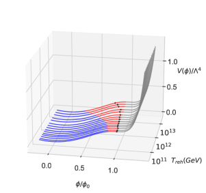
Figure 2: The inflaton potential (5) is divided into three color-coded regions; tachyonic instability (red), parametric resonance (blue), and no amplification of the electromagnetic fields (gray). The border between the gray and red regions is determined by the criterion $g|\dot{\phi}|\geq 2H$. Each line represents a different choice of $\phi_{0}$, resulting in a different value of $T_{\rm reh}$. As $T_{\rm reh}$ decreases, the red region shrinks and tachyonic amplification tends to be less efficient. Black dots denote the end of inflation, $\dot{H}=-H^{2}$.

For the $\text{U}(1)_{\text{em}}$ gauge field, we choose the radiation gauge, $A_{0}=0$ and $\nabla\cdot\bm{A}=0$, and quantize it as

$$A_{i}(t,\bm{x})= \sum_{\lambda=\pm}\int\frac{{\rm d}^{3}k}{(2\pi)^{3}}e^{i\bm{k\cdot x}}$$

$$\times e_{i}^{(\lambda)}(\hat{\bm{k}})\left[\hat{b}_{\bm{k}}^{(\lambda)}\mathcal{A}_{\lambda}(k,t)+\hat{b}_{-\bm{k}}^{(\lambda){\dagger}}\mathcal{A}_{\lambda}^{*}(k,t)\right],$$ (6)

where $\bm{e}^{(\pm)}(\hat{\bm{k}})$ is a circular-polarization vector with the comoving wavenumber ${\bm{k}}$, $\hat{b}_{\bm{k}}^{(\lambda){\dagger}}$ and $\hat{b}_{\bm{k}}^{(\lambda)}$ are standard creation and annihilation operators, respectively, and $\mathcal{A}_{\lambda}(k,t)$ is a mode function satisfying

$$\ddot{\mathcal{A}}_{\pm}+H\dot{\mathcal{A}_{\pm}}+\frac{k}{a}\left(\frac{k}{a}\mp g\dot{\phi}\right)\mathcal{A}_{\pm}=0.$$ (7)

In this model, the electromagnetic fields experience two distinct stages of the amplification [12, 13, 14]: (i) When the inflaton velocity is large enough to satisfy the inequality $g|\dot{\phi}|\gtrsim 2H$, either of two circular-polarization modes $\mathcal{A}_{\pm}$ effectively obtains a negative mass squared (i.e., the parenthesis in Eq. (7) becomes negative) and grows due to tachyonic instability. (ii) While the inflaton oscillates after inflation, parametric resonance takes place and both polarization modes are equally amplified. We emphasize that the helicity of the magnetic field (i.e., a significant imbalance between $\mathcal{A}_{+}$ and $\mathcal{A}_{-}$) is produced only in the first stage.

Once $\mathcal{A}_{\pm}(k,t)$’s are computed, the comoving magnetic field strength and its coherence length are evaluated, respectively, as

$$\tilde{B}^{2}(t) \equiv a^{4}B^{2}=\int\frac{\differential^{3}k}{(2\pi)^{3}}\,k^{2}\Big{(}|\mathcal{A}_{+}|^{2}+|\mathcal{A}_{-}|^{2}\Big{)}\,,$$ (8)

$$\tilde{\lambda}(t) \equiv\frac{\lambda}{a}=\frac{\int\differential^{3}k\,(2\pi/k)\,k^{2}\left(|\mathcal{A}_{+}|^{2}+|\mathcal{A}_{-}|^{2}\right)}{\int\differential^{3}k\,k^{2}\left(|\mathcal{A}_{+}|^{2}+|\mathcal{A}_{-}|^{2}\right)}\,.$$ (9)

We also pay particular attention to the helicity fraction,

$$\chi(t)\equiv\frac{\int\frac{\differential^{3}k}{(2\pi)^{3}}\,k\Big{(}|\mathcal{A}_{-}|^{2}-|\mathcal{A}_{+}|^{2}\Big{)}}{\int\frac{\differential^{3}k}{(2\pi)^{3}}\,k\Big{(}|\mathcal{A}_{-}|^{2}+|\mathcal{A}_{+}|^{2}\Big{)}}\,,$$ (10)

where $\chi$ indicates how helical the magnetic fields are, and $\chi=\pm 1$ corresponds to maximally helical magnetic fields.

For simplicity, we assume that the inflaton instantaneously decays into radiation at $H_{\rm reh}$. Then, we can approximate the reheating temperature as $T_{\rm reh}\simeq\quantity[90M_{\rm Pl}^{2}H_{\rm reh}^{2}/(100\pi^{2})]^{1/4}$ [32], with the scale factor $a_{\rm reh}\simeq 5.5\times 10^{-32}\sqrt{M_{\rm Pl}/H_{\rm reh}}$, where $M_{\rm Pl}$ is the reduced Planck mass. We ignore the effect of charged particles before the reheating completion.

IV IV. Numerical calculation

We numerically solve Eqs. (3) and (7) combined with the Friedmann equation, $3M_{\rm Pl}^{2}H^{2}\simeq\rho_{\phi}$, until the magnetic field generation weakens and the energy fraction starts decreasing. The background inflaton reaches the inflationary attractor before the horizon-crossing of the CMB modes. Note that the electromagnetic fields are initially in the Bunch-Davies vacuum. We repeatedly run simulations by varying the model parameters corresponding to different reheating temperatures $T_{\rm reh}$. In Appendix. A, we give the parameter sets used in our calculations and describe our parameter selection strategy.

We are interested in $\tilde{B}^{2}\tilde{\lambda}$ to which the blazer observations are sensitive. In Fig. 3, we present our numerical result of $\tilde{B}^{2}\tilde{\lambda}(t_{\rm reh})$ versus the Hubble parameter $H_{\rm reh}$ at the temperature $T_{\rm reh}$. We also plot $\chi\tilde{B}^{2}\tilde{\lambda}(t_{\rm reh})$ and an analytic estimate of $\tilde{B}^{2}\tilde{\lambda}(t_{\rm reh})$, which is derived as follows. The inflaton equation of motion is given by $\partial_{\mu}\quantity[a^{3}\partial^{\mu}\phi-(g/2)\epsilon^{\mu\nu\rho\sigma}A_{\nu}\partial_{\rho}A_{\sigma}]=a^{3}\partial_{\phi}V$. Note that the second term on the left-hand side was neglected in Eq. (3), whose approximation assumes that $|a^{3}\dot{\phi}|\gg|(g/2)\epsilon^{0\nu\rho\sigma}A_{\nu}\partial_{\rho}A_{\sigma}|$. The homogeneous oscillating inflaton at $t_{\rm reh}$ is approximately given by $|\dot{\phi}|\simeq\sqrt{3}M_{\rm Pl}H_{\rm reh}$. As a large-volume average, we have $|\epsilon^{0\nu\rho\sigma}A_{\nu}\partial_{\rho}A_{\sigma}|\simeq\chi\tilde{B}^{2}\tilde{\lambda}/2\pi$. However, if the magnetic fields are non-helical ($|\chi|\ll 1$), it would underestimate its local value. Local fluctuations yield $|\epsilon^{0\nu\rho\sigma}A_{\nu}\partial_{\rho}A_{\sigma}|\simeq\sqrt{\langle\left(\epsilon^{0\nu\rho\sigma}A_{\nu}\partial_{\rho}A_{\sigma}\right)^{2}\rangle}\simeq\tilde{B}^{2}\tilde{\lambda}/2\pi$, which could dominate the homogeneous value. Thus, we adopt the latter and obtain a generic upper bound as

$$\tilde{B}^{2}_{\rm reh}\tilde{\lambda}_{\rm reh}\lesssim\gamma,\quad\gamma\equiv\frac{4\sqrt{3}\pi}{g}a_{{\rm reh}}^{3}M_{\rm Pl}H_{\rm reh}.$$ (11)

From Eq. (4), the actual values of $\tilde{B}^{2}_{\rm reh}\tilde{\lambda}_{\rm reh}$ are expected to be of the order of $\epsilon\gamma$. In Fig. 3, we see an excellent agreement between this analytical estimate (green) and the numerical results (blue).

Figure 3: The numerical results for $\tilde{B}^{2}_{\rm reh}\tilde{\lambda}_{\rm reh}$ (blue) and $\chi_{\rm reh}\tilde{B}^{2}_{\rm reh}\tilde{\lambda}_{\rm reh}$ (red) against $H_{\rm reh}$. An analytic estimate for $\tilde{B}^{2}_{\rm reh}\tilde{\lambda}_{\rm reh}$ (green) derived below Eq. (11) agrees well with the former. For $H_{\rm reh}\lesssim 10^{6}~{}{\rm GeV}$, the helicity fraction $\chi_{\rm reh}$ significantly decreases from unity as $H_{\rm reh}$ decreases.

As seen in Fig. 3, the produced magnetic fields are significantly non-helical ($\chi\ll 1$) for $H_{\rm reh}\ll 10^{6}~{}{\rm GeV}$. This is because the amplification during the first stage due to tachyonic instability is no longer efficient and the magnetic fields are mostly generated by parametric resonance in the second stage for low reheating temperatures. In Fig. 2, we plot the region of the potential in which tachyonic instability occurs before the end of inflation, namely $g|\dot{\phi}|\geq 2H$. Such a region shrinks as $T_{\rm reh}$ decreases because inflation ends with the rapid growth of $|\dot{\phi}|$, and then the inflaton immediately starts oscillating, as is typical in small-field models. In Fig. 4, we show the numerical evolution for $\phi(t)$ and $\chi(t)$ in an intermediate case where $\chi$ converges to $\simeq 0.5$. The helicity fraction $\chi$ rapidly oscillates in phase with the inflaton, which indicates that the magnetic fields are generated primarily by parametric resonance. Nevertheless, the final value of $\chi$ is determined by the imbalance between the two circular-polarization modes produced by relatively inefficient tachyonic instability, since parametric resonance equally amplifies both of the modes.

In much lower $T_{\rm reh}$ cases, it is numerically challenging to track the extreme slow-roll evolution and obtain fine-tuned values of $\alpha$ as pointed out in [30]. To extrapolate them to lower $T_{\rm reh}$, we find fitting functions of the comoving magnetic-field amplitude, comoving coherence length, and helicity fraction, as (see Appendix. B for details)

$$\tilde{B}_{\rm reh} \simeq 7.0\times 10^{-7}~{}\text{G}\,,$$ (12)

$$\tilde{\lambda}_{\rm reh} \simeq 2.7\times 10^{-14}~{}{\rm Mpc}\quantity(\frac{T_{\rm reh}}{100~{}{\rm GeV}})^{-0.68}\,,$$ (13)

$$\chi_{\rm reh} \simeq 3.1\times 10^{-6}\quantity(\frac{T_{\rm reh}}{100~{}{\rm GeV}})^{0.55}\,,$$ (14)

for $T_{\rm reh}\ll 10^{12}~{}{\rm GeV}$. For the fitting of $\chi_{\rm reh}$, we used only the numerical results of the parameteric-resonance dominant regime ($H_{\rm reh}\leq 10^{6}~{}{\rm GeV}$), while we exploited all the data points for the $\tilde{\lambda}_{\rm reh}$ fitting. $\tilde{B}_{\rm reh}$ does not depend on $T_{\rm reh}$, because $B_{\rm reh}\propto\sqrt{2\epsilon\rho_{\phi,{\rm reh}}}\propto H_{\rm reh}$ and $a_{\rm reh}\propto H_{{\rm reh}}^{-1/2}$ are cancelled out. As $T_{\rm reh}$ decreases, we are left with a smaller residual difference in the almost equally produced two circular-polarization modes of the magnetic fields, which leads to $\chi_{\rm reh}\propto T_{\rm reh}^{0.55}$ in Eq. (14).

Figure 4: The time evolution of the homogeneous inflaton $\phi$ (orange) and the helicity fraction $\chi$ (blue) in an intermediate case of $T_{\rm reh}\simeq 10^{11}{\rm GeV}$. In such a case, tachyonic instability generates only $\mathcal{O}(1)$ imbalance of two circular-polarization modes (e.g., $|\mathcal{A}_{-}|=2|\mathcal{A}_{+}|$) until the inflaton oscillation begins. For each half oscillation, parametric resonance alternately amplifies $\mathcal{A}_{-}$ and $\mathcal{A}_{+}$ by up to $\mathcal{O}(10)$ and $\chi$ flips its sign. As the inflaton amplitude decreases, parametric resonance becomes less effective and $\chi$ converges to an $\mathcal{O}(1)$ value. For lower (higher) $T_{\rm reh}$, the effect of tachyonic instability is less (more) significant, which leads to $\chi\ll 1\ (\chi\simeq 1)$.

Before turning to our main results, we consider maximizing the produced magnetic fields by slightly modifying the inflaton potential. To maintain the tachyonic instability region of the potential even for very low $T_{\rm reh}$, we attach a quadratic function to the potential (5) as

$$V_{\rm mod}(\phi)=\begin{cases}V(\phi-\phi_{1})&({\rm for}~{}\phi-\phi_{1}\geq\phi_{f})\\ m_{0}^{2}\phi^{2}/2&({\rm for}~{}\phi-\phi_{1}<\phi_{f})\end{cases},$$ (15)

where $m_{0}\equiv\Lambda^{2}/(100\phi_{0})$, $\phi_{f}$ denotes $\phi$ at the end of inflation, and $\phi_{1}$ is the appropriate shift for the two parts of the potential to be smoothly connected at $\phi_{f}$. $\phi_{1}$ is uniquely determined by matching the potential at $\phi_{f}$. Right after inflation ends, the inflaton gently rolls down on $m_{0}^{2}\phi^{2}/2$ where tachyonic instability efficiently occurs irrespective of $T_{\rm reh}$. The shrinkage of the red region seen in Fig. 2 does not occur in this case. We numerically show that our scenario with this new potential always produces fully helical magnetic fields with $\chi=1$. $\tilde{B}_{\rm reh}$ is the same as Eq. (12), and we fit (see Appendix. B for details)

$$\tilde{\lambda}_{\rm reh}=1.4\times 10^{-14}~{}{\rm Mpc}\quantity(\frac{T_{\rm reh}}{100{\rm GeV}})^{-0.57}.$$ (16)

Although the modified potential (15) is somewhat artificial, the implications of examining it are twofold: first, to validate our understanding of why $\chi_{\rm reh}$ reduces as $T_{\rm reh}$ decreases in the original case and second, to provide an example of single-field inflation models generating much stronger magnetic fields than the previous case.

V V. Magnetic fields at present time

Summarizing the results so far, either of Eqs. (12), (13), and (14) or Eqs. (12), (16), and $\chi_{\rm reh}=1$ set the initial conditions for the subsequent evolution of magnetic fields. Now, let us discuss the implication of these results in light of observational constraints on the cosmological magnetic field in today’s universe.

In tracking the evolution until the recombination epoch, we can use the magnetic helicity conservation due to the large electric conductivity [1],

$$\chi\tilde{B}^{2}\tilde{\lambda}=\text{const.}\qquad(t_{\rm reh}\leq t\leq t_{\rm rec})\,.$$ (17)

The MHD analysis has provided another condition at the recombination time $t_{\rm rec}$ [24, 26],

$$\left(\dfrac{\tilde{B}_{\text{rec}}}{10^{-12}\;\text{G}}\right)^{2}\left(\dfrac{\tilde{\lambda}_{\text{rec}}}{10^{-8}\;\text{Mpc}}\right)^{-1}\sim 1\,,$$ (18)

which is shown as a blue line in Fig. 1. Since maximally helical magnetic fields keep $|\chi|=1$ during the evolution, the above two equations suffice to determine $\tilde{B}_{\rm rec}$ and $\tilde{\lambda}_{\text{rec}}$ independently for the modified potential (15) with $\chi_{\rm reh}=1$.

If $\chi_{\rm reh}<1$, however, we need yet another equation to find $B_{\rm rec},\lambda_{\rm rec}$ and $\chi_{\rm rec}$. Recently, it has been pointed out that the Hosking integral is conserved for non-helical magnetic fields [33, 34, 35],

$$\tilde{B}^{4}_{\rm reh}\tilde{\lambda}^{5}_{\rm reh}=\text{const.}\qquad(t_{\rm reh}\leq t\leq t_{\rm rec},\,|\chi|\ll 1).$$ (19)

For maximally helical magnetic fields, the Hosking integral is ill-defined and hence this constraint is irrelevant. Although it is not well-established how partially helical magnetic fields (e.g., $|\chi|=\mathcal{O}(0.1)$) behave, we assume that Eq. (19) holds [26].

Combining Eqs. (17), (18) and (19), we obtain

$$\left(\tilde{B}_{\text{rec}}/10^{-12}\;\text{G},\ \tilde{\lambda}_{\text{rec}}/10^{-8}\;\text{Mpc}\right)$$

$$\sim\left\{\begin{array}[]{cc}\left(1\times\mathcal{T}_{\rm reh}^{-0.03},\,2\times\mathcal{T}_{\rm reh}^{-0.07}\right)&(T_{\rm reh}\lesssim 570{\rm MeV})\\[4.0pt] \left(0.5\times\mathcal{T}_{\rm reh}^{-0.24},\,0.2\times\mathcal{T}_{\rm reh}^{-0.49}\right)&(T_{\rm reh}\gtrsim 570{\rm MeV})\\[4.0pt] \left(30\times\mathcal{T}_{\rm reh}^{-0.14},\,800\times\mathcal{T}_{\rm reh}^{-0.29}\right)&({\rm modified\ model})\end{array}\right.,$$ (23)

with $\mathcal{T}_{\rm reh}\equiv T_{\text{reh}}/100\,\text{GeV}<1$. Their evolution paths and the resultant magnetic fields are shown in Fig. 1. Note that, for the GMSSM model (5) with relatively high reheating temperatures, $T_{\text{reh}}\gtrsim 570\;\text{MeV}$, the magnetic fields become maximally helical by the recombination. In such cases, if Eq. (19) yields $\chi_{\rm rec}>1$, we use only Eqs. (17) and (18) with $\chi_{\rm rec}=1$.

We expect that the intergalactic magnetic fields in the void remain frozen in the comoving sense after the recombination epoch. Thus we identify their present strength and coherence length with the comoving ones at recombination, $B_{0}=\tilde{B}_{\rm rec}$ and $\lambda_{0}=\tilde{\lambda}_{\rm rec}$. Now, our results are compared to the latest observational constraint [4],

$$\left(\dfrac{B_{0}}{2\times 10^{-17}\;\text{G}}\right)^{2}\left(\dfrac{\lambda_{0}}{0.2\;\text{Mpc}}\right)\gtrsim 1~{}~{}\;\text{for}\,\;\lambda_{0}\ll 0.2\;\text{Mpc}.$$ (24)

As seen in Fig. 1, our scenario satisfies this constraint for any $T_{\rm reh}<100~{}{\rm GeV}$ and thus successfully explains the origin of cosmological magnetic fields.

VI VI. Conclusion

In this paper, we have proposed an inflationary magnetogenesis scenario that is consistent with current observations. Our scenario can explain the origin of the void magnetic field without producing baryon isocurvature perturbations. The key point is that primordial magnetogenesis occurs below the electroweak scale, which makes the baryon isocurvature problem irrelevant. We have performed numerical simulations for low-energy inflation potentials, and successfully produced magnetic fields that exceed the blazar constraint.

Although our results capture the universal properties of low-energy magnetogenesis scenarios, calculations for other kinds of potentials, especially more natural ones that realize $\chi_{\rm reh}=1$, would be interesting. Furthermore, by taking into account the backreaction [11, 12, 13, 14], Schwinger effect [17, 18], and the electric conductivity of the universe [36, 37], more precise results will be obtained in the numerical simulation. We leave these issues for future works.

VII Acknowledgement

The work is supported by JSPS KAKENHI Grant Nos. JP23KJ0642 (F.U.), JP23K03424, JP20H05854 (T.F.), JP22K03642 (S.T.) and also by the Forefront Physics and Mathematics Program to Drive Transformation (F.U.) and Waseda University Special Research Project No. 2023C-473 (S.T.).

Appendix A Appendix A: Parameters

Here we describe the way to choose parameters for the numerical calculations. The inflaton potential must be consistent with the observed data of CMB temperature anisptropies. Once we fix $\phi_{0}$ in Eq. (5), $\alpha$ is almost uniquely determined by requiring the agreement with the observed spectral index $n_{s}$ of scalar perturbations. It must be in the range of $n_{s}=0.966\pm 0.004$ [38], and $\alpha$ needs to be severely fine-tuned as mentioned previously. Also, the value of $\Lambda$ is determined by the CMB constraint on the amplitude of curvature perturbations. The upper bound on the tensor-to-scalar ratio is trivially satisfied due to a small slow-roll parameter during inflation.

The remaining parameter is the Chern-Simons coupling constant, $g$. To fix this value, we define $t_{\rm reh}$ as the time at which each magnetic field strength reaches its maximum, and we repeat the calculations for different coupling constants $g$. Then, we find the appropriate value of $g$ satisfying the condition $\epsilon(t_{\rm reh})=0.1$. The parameters we used for the GMSSM potential (5) are shown in Tab. I. The ones for the modified potential (15) are also given in Tab. II.

$\phi_{0}/M_{\rm Pl}$	$gM_{\rm Pl}$	$1-\alpha$
0.013	105.2	$1.0\times 10^{-13}$
0.016	97.30	$2.0\times 10^{-13}$
0.020	87.60	$5.0\times 10^{-13}$
0.025	79.90	$1.1\times 10^{-12}$
0.030	74.00	$2.4\times 10^{-12}$
0.040	65.90	$7.0\times 10^{-12}$
0.050	60.20	$1.9\times 10^{-11}$
0.070	53.50	$6.5\times 10^{-11}$
0.100	46.40	$2.8\times 10^{-10}$
0.140	40.18	$9.8\times 10^{-10}$
0.220	33.55	$6.0\times 10^{-9}$
0.300	29.90	$2.0\times 10^{-8}$
0.500	24.70	$1.4\times 10^{-7}$
0.700	21.40	$6.0\times 10^{-7}$
1.000	18.65	$2.3\times 10^{-6}$

Table 1: The parameters used for the numerical calculations of the GMSSM potential (5).

$\phi_{0}/M_{\rm Pl}$	$gM_{\rm Pl}$	$1-\alpha$
0.013	29.90	$1.0\times 10^{-13}$
0.016	27.53	$2.0\times 10^{-13}$
0.020	25.38	$5.0\times 10^{-13}$
0.025	23.35	$1.3\times 10^{-12}$
0.030	21.45	$2.4\times 10^{-12}$
0.040	18.74	$7.0\times 10^{-12}$
0.050	17.36	$1.9\times 10^{-11}$
0.070	16.85	$6.4\times 10^{-11}$
0.100	16.50	$2.8\times 10^{-10}$
0.140	16.25	$9.8\times 10^{-10}$

Table 2: The parameters used for the modified potential (15).

Appendix B Appendix B: The extrapolated results

To obtain the values of the comoving coherence length $\tilde{\lambda}_{\rm reh}$ and the helicity fraction $\chi_{\rm reh}$ for lower $T_{\rm reh}$, we extrapolate the numerical results by assuming that they are power-law functions of $T_{\rm reh}$. The fitting functions given by Eqs. (13) and (14) are shown in Figs. 5 and 6, respectively. While we use all the points in Fig. 5 for fitting $\tilde{\lambda}_{\rm reh}$, we only use 9 data points on the low $T_{\rm reh}$ side for fitting $\chi_{\rm reh}$ in Fig. 6, which follows a power-law relation.

Figure 5: The relation between the comoving coherence length $\tilde{\lambda}_{\rm reh}$ and reheating temperature $T_{\rm reh}$. The blue solid line shows the fitting function given by Eq. (13).

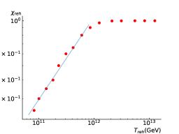
Figure 6: The relation between the helicity fraction $\chi_{\rm reh}$ and $T_{\rm reh}$. The helicity fraction saturates at unity for $T_{\rm reh}\gtrsim 10^{12}$ GeV. For lower reheating temperatures, $\chi_{\rm reh}$ exhibits the power-law behavior.

Similarly, we extrapolate $\tilde{\lambda}_{\rm reh}$ for the modified potential (15) and obtain the fitting formula (16) shown in Fig. 7. Note that $\chi_{\rm reh}$ is always unity and we do not need to extrapolate it in this model.

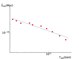
Figure 7: The relation between the comoving coherence length $\tilde{\lambda}_{\rm reh}$ and reheating temperature $T_{\rm reh}$ for the potential (15).

References

- [1] Ruth Durrer and Andrii Neronov. Cosmological magnetic fields: their generation, evolution and observation. The Astronomy and Astrophysics Review, 21:62, June 2013.
- [2] A. Neronov and I. Vovk. Evidence for strong extragalactic magnetic fields from fermi observations of tev blazars. Science, 328:73–75, 2010.
- [3] M. Ackermann et al. The search for spatial extension in high-latitude sources detected by the fermi large area telescope. ApJS, 237(2):32, 2018.
- [4] V. A. Acciari et al. A lower bound on intergalactic magnetic fields from time variability of 1ES 0229+200 from MAGIC and Fermi/LAT observations. Astron. Astrophys., 670:A145, 2023.
- [5] K. Dolag, M. Kachelriess, S. Ostapchenko, and R. Tomas. Lower limit on the strength and filling factor of extragalactic magnetic fields. Astrophys. J. Lett., 727:L4, 2011.
- [6] Kyrylo Bondarenko, Alexey Boyarsky, Alexander Korochkin, Andrii Neronov, Dmitri Semikoz, and Anastasia Sokolenko. Account of the baryonic feedback effect in -ray measurements of intergalactic magnetic fields. Astron. Astrophys., 660:A80, 2022.
- [7] Axel Brandenburg and Kandaswamy Subramanian. Astrophysical magnetic fields and nonlinear dynamo theory. Phys. Rept., 417:1–209, 2005.
- [8] Michael S Turner and Lawrence M Widrow. Inflation-produced, large-scale magnetic fields. Physical Review D, 37(10):2743, 1988.
- [9] Bharat Ratra. Cosmological’seed’magnetic field from inflation. The Astrophysical Journal, 391:L1–L4, 1992.
- [10] W Daniel Garretson, George B Field, and Sean M Carroll. Primordial magnetic fields from pseudo goldstone bosons. Physical Review D, 46(12):5346, 1992.
- [11] Kazuharu Bamba and J. Yokoyama. Large scale magnetic fields from inflation in dilaton electromagnetism. Phys. Rev. D, 69:043507, 2004.
- [12] Tomohiro Fujita, Ryo Namba, Yuichiro Tada, Naoyuki Takeda, and Hiroyuki Tashiro. Consistent generation of magnetic fields in axion inflation models. JCAP, 05:054, 2015.
- [13] Peter Adshead, John T. Giblin, Timothy R. Scully, and Evangelos I. Sfakianakis. Magnetogenesis from axion inflation. JCAP, 10:039, 2016.
- [14] Jose Roberto Canivete Cuissa and Daniel G. Figueroa. Lattice formulation of axion inflation. Application to preheating. JCAP, 06:002, 2019.
- [15] Vittoria Demozzi, Viatcheslav Mukhanov, and Hector Rubinstein. Magnetic fields from inflation? JCAP, 08:025, 2009.
- [16] Neil Barnaby, Ryo Namba, and Marco Peloso. Observable non-gaussianity from gauge field production in slow roll inflation, and a challenging connection with magnetogenesis. Phys. Rev. D, 85:123523, 2012.
- [17] O. O. Sobol, E. V. Gorbar, M. Kamarpour, and S. I. Vilchinskii. Influence of backreaction of electric fields and Schwinger effect on inflationary magnetogenesis. Phys. Rev. D, 98(6):063534, 2018.
- [18] E. V. Gorbar, K. Schmitz, O. O. Sobol, and S. I. Vilchinskii. Gauge-field production during axion inflation in the gradient expansion formalism. Phys. Rev. D, 104(12):123504, 2021.
- [19] Kohei Kamada, Fumio Uchida, and Jun’ichi Yokoyama. Baryon isocurvature constraints on the primordial hypermagnetic fields. JCAP, 04:034, 2021.
- [20] Mohamed M. Anber and Lorenzo Sorbo. N-flationary magnetic fields. JCAP, 10:018, 2006.
- [21] Ricardo J. Z. Ferreira, Rajeev Kumar Jain, and Martin S. Sloth. Inflationary Magnetogenesis without the Strong Coupling Problem II: Constraints from CMB anisotropies and B-modes. JCAP, 06:053, 2014.
- [22] Tomohiro Fujita and Ryo Namba. Pre-reheating Magnetogenesis in the Kinetic Coupling Model. Phys. Rev. D, 94(4):043523, 2016.
- [23] Takeshi Kobayashi and Martin S. Sloth. Early Cosmological Evolution of Primordial Electromagnetic Fields. Phys. Rev. D, 100(2):023524, 2019.
- [24] David N. Hosking and Alexander A. Schekochihin. Cosmic-void observations reconciled with primordial magnetogenesis. arXiv e-prints, page arXiv:2203.03573, March 2022.
- [25] Fumio Uchida, Motoko Fujiwara, Kohei Kamada, and Jun’ichi Yokoyama. New description of the scaling evolution of the cosmological magneto-hydrodynamic system. Physics Letters B, 843:138002, August 2023.
- [26] F. Uchida, M. Fujiwara, K. Kamada, and J. Yokoyama. in preperation.
- [27] Kohei Kamada and Andrew J. Long. Evolution of the Baryon Asymmetry through the Electroweak Crossover in the Presence of a Helical Magnetic Field. Phys. Rev. D, 94(12):123509, 2016.
- [28] Kohei Kamada and Andrew J. Long. Baryogenesis from decaying magnetic helicity. Phys. Rev. D, 94(6):063501, 2016.
- [29] Keisuke Inomata, Masahiro Kawasaki, Alexander Kusenko, and Louis Yang. Big Bang Nucleosynthesis Constraint on Baryonic Isocurvature Perturbations. JCAP, 12:003, 2018.
- [30] Jerome Martin, Christophe Ringeval, and Vincent Vennin. Encyclopædia inflationaris. Physics of the Dark Universe, 5:75–235, 2014.
- [31] David H Lyth. Mssm inflation. Journal of Cosmology and Astroparticle Physics, 2007(04):006, 2007.
- [32] Edward W Kolb, Alessio Notari, and Antonio Riotto. Reheating stage after inflation. Physical Review D, 68(12):123505, 2003.
- [33] David N. Hosking and Alexander A. Schekochihin. Reconnection-Controlled Decay of Magnetohydrodynamic Turbulence and the Role of Invariants. Physical Review X, 11(4):041005, October 2021.
- [34] Hongzhe Zhou, Ramkishor Sharma, and Axel Brandenburg. Scaling of the Hosking integral in decaying magnetically dominated turbulence. Journal of Plasma Physics, 88(6):905880602, December 2022.
- [35] Axel Brandenburg and Gustav Larsson. Turbulence with Magnetic Helicity That Is Absent on Average. Atmosphere, 14(6):932, May 2023.
- [36] Bruce A. Bassett, Giuseppe Pollifrone, Shinji Tsujikawa, and Fermin Viniegra. Preheating as cosmic magnetic dynamo. Phys. Rev. D, 63:103515, 2001.
- [37] Tomohiro Fujita and Ruth Durrer. Scale-invariant Helical Magnetic Fields from Inflation. JCAP, 09:008, 2019.
- [38] Planck Collaboration. Planck 2018 results. VI. Cosmological parameters. Astronomy & Astrophysics, 641:A6, September 2020.