A feasible method for general convex low-rank SDP problems

Abstract

In this work, we consider the low rank decomposition (SDPR) of general convex semidefinite programming problems (SDP) that contain both a positive semidefinite matrix and a nonnegative vector as variables. We develop a rank-support-adaptive feasible method to solve (SDPR) based on Riemannian optimization. The method is able to escape from a saddle point to ensure its convergence to a global optimal solution for generic constraint vectors. We prove its global convergence and local linear convergence without assuming that the objective function is twice differentiable. Due to the special structure of the low-rank SDP problem, our algorithm can achieve better iteration complexity than existing results for more general smooth nonconvex problems. In order to overcome the degeneracy issues of SDP problems, we develop two strategies based on random perturbation and dual refinement. These techniques enable us to solve some primal degenerate SDP problems efficiently, for example, Lovász theta SDPs. Our work is a step forward in extending the application range of Riemannian optimization approaches for solving SDP problems. Numerical experiments are conducted to verify the efficiency and robustness of our method.

keywords: semidefinte programming, feasible method, Riemannian optimization
Mathematics subject classification: 90C06, 90C22, 90C30

1 Introduction

1.1 Low rank SDP problem

The standard linear SDP problem is as follows:

$$\min\left\{\big{\langle}C,X\big{\rangle}:\ \mathcal{A}(X)=b,\ X\in\mathbb{S}^{n}_{+}\right\},$$ (1)

where $C\in\mathbb{S}^{n},$ $b\in\mathbb{R}^{m}$ and $\mathcal{A}:\mathbb{S}^{n}\rightarrow\mathbb{R}^{m}$ is a linear mapping. Problem (1) can be solved with guaranteed convergence by many well-developed convex solvers like SDPT3 [47, 48], MOSEK [5] and SDPNAL [44, 56, 61]. However, due to the dimensionality of $O(n^{2})$ of the matrix variable, convex solvers are inefficient when $n$ is large. To overcome this issue, Burer and Monteiro [19, 20] proposed the following low rank decomposition of (1), which we also call as the factorized model:

$$\min\left\{\big{\langle}C,RR^{\top}\big{\rangle}:\ \mathcal{A}(RR^{\top})=b,\ R\in\mathbb{R}^{n\times r}\right\}.$$ (2)

From the well known low rank property of problem (1) [8, 25, 40], problem (1) and (2) are equivalent when $r(r+1)/2\geq m.$ By choosing $r=\lceil\sqrt{2m}\rceil,$ the dimension of (2) becomes $O(nm^{1/2}),$ which is much smaller than $O(n^{2})$ if $m=o(n^{2}).$

1.2 Feasible method and its limitation

There are mainly two types of methods to solve (2). One is augmented Lagrangian method (ALM). It has been implemented as a general linear SDP solver by Burer and Monteiro. The other one is feasible method based on Riemannian optimization (see [7, 13, 31, 53]). This method assumes that the feasible set of (2) is a Riemannian manifold. Thus, one can use Riemannian optimization method such as Riemannian gradient descent and Riemannian trust region method to solve the problem [1, 14, 16, 33, 54, 55]. Apart from ALM and Riemannian optimization methods, Bellavia et al. [9] developed a rank-adaptive interior point method for low-rank linear SDP problems and applied it to matrix completion problems.

It is well-known that the efficiency of ALM relies heavily on the penalty parameter and the termination criterion for solving its subproblems. Compared with ALM, feasible method is penalty-free and one can directly decrease the objective function value on the manifold just like unconstrained optimization. Another advantage of feasible method is that it can find a solution of acceptable accuracy after only a few iterations while the primal feasibility is maintained. However, the application range of feasible method is quite narrow. As far as we know, feasible method has never been used in a general SDP solver like interior point method and ALM. Current feasible method is mainly designed for SDP problems with block-diagonal equality constraints such as the SDP relaxations of max-cut problems, robust PCA and synchronization of rotations [13, 24]. The feasible sets of such SDP problems are simple smooth manifolds like oblique manifold and Stiefel manifold. Different from these special problems, the constraints of a general SDP problem may be more complicated with inequality constraints and its feasible set may contain singular points. The worst case is that the optimal solution lies exactly on a singular point. This will cause numerical issues as the iteration points approach it. Recently, Wang et al. [51] and Wen et al. [52] developed Riemannian ALMs that solve (2) by separating its constraints into two parts such that one of them is a Riemannian manifold. These methods are not feasible methods and the manifolds they considered are still the special manifolds just mentioned above. In [45, 46], we have applied a feasible method with rounding and escaping strategy to solve some special SDP problems with finite number of singular points. However, for a general SDP problem, there might be infinite number (even uncountable) of singular points. It would be challenging to extend that idea to general SDP problems.

In this paper, our goal is to demonstrate that feasible methods can also be developed to solve a general SDP problem. However, we should emphasize that unlike other previous works on Riemannian optimization approaches for solving an SDP with special constraints, we target SDP problems with general linear constraints and the corresponding feasible sets of the factorized problems (2) are algebraic varieties rather than special manifolds. Thus, even though our rank-support-adaptive feasible method is motivated by Riemannian optimization approaches, we must overcome the inherent theoretical and numerical difficulties brought about by singular points in the feasible sets. In these aspects, our design of the feasible method for solving (2), and its theoretical analysis and numerical implementation, are much more challenging than many existing works which target only SDP problems with special constraints. We will state our contributions and their relationship to existing works in the literature in the following subsections.

1.3 A general SDP model and its low rank decomposition

We consider the following convex (possibly nonlinear) SDP problem:

$$({\rm SDP})\ \min\left\{\phi(X,x):\ \mathcal{K}(X,x)=b,\ X=\begin{pmatrix}I_{k}&*\\ *&*\end{pmatrix}\in\mathbb{S}_{+}^{n},\ x\in\mathbb{R}^{p}_{+}\right\}.$$ (3)

In (SDP), $\phi:\mathbb{S}^{n}\times\mathbb{R}^{p}\rightarrow\mathbb{R}$ is a convex continuously differentiable function, $b\in\mathbb{R}^{m}$, $\mathcal{K}:\mathbb{S}^{n}\times\mathbb{R}^{p}\rightarrow\mathbb{R}^{m}$ is a linear mapping such that for any $(X,x)\in\mathbb{S}^{n}\times\mathbb{R}^{p},$

$$\mathcal{K}\left(X,x\right):=\mathcal{A}(X)+Bx,$$ (4)

where $B\in\mathbb{R}^{m\times p}$ and $\mathcal{A}:\mathbb{S}^{n}\rightarrow\mathbb{R}^{m}$ is a linear mapping such that

$$\mathcal{A}(X):=\left(\big{\langle}A_{1},X\big{\rangle},\big{\langle}A_{2},X\big{\rangle},\ldots,\big{\langle}A_{m},X\big{\rangle}\right)^{\top}$$

for data matrices $A_{1},A_{2},\ldots,A_{m}\in\mathbb{S}^{n}.$ (SDP) is more general than problem (1) because the objective function may not be linear and there is an additional nonnegative vector variable $x\in\mathbb{R}^{p}_{+}.$ This vector variable may occur in SDP problems with inequality constraints, where it is used as the slack variable. Note that (SDP) has an implicit fixed constraint given by $X_{1:k,1:k}=I_{k},$ but the case where $k=0$ is allowed. This constraint, with $k=1$, appears in the SDP relaxations of quadratically constrained quadratic programming with linear terms [4]. We intentionally separate the fixed constraints from $\mathcal{A}\left(X\right)=b$ because of its special structure. Now, we consider the following low rank decomposition of (SDP):

$$({\rm SDPR})\ \min\left\{\phi\big{(}\widehat{R}\widehat{R}^{\top},y\circ y\big{)}:\ \mathcal{K}\big{(}\widehat{R}\widehat{R}^{\top},y\circ y\big{)}=b,\widehat{R}=[I_{k,r};R]\in\mathbb{R}^{n\times r},\ y\in\mathbb{R}^{p}\right\},$$

where $k\leq r\leq n$, “$\circ$” denotes the Hadamard product and $I_{k,r}=[I_{k},0_{k\times(r-k)}]$. In (SDPR), we consider $R\in\mathbb{R}^{(n-k)\times r}$ and $y\in\mathbb{R}^{p}$ as unknown variables. Different from the traditional Burer-Monteiro factorization, we fixed the first $k$ rows of the factorized matrix to be the $k$ by $r$ identity matrix $I_{k,r}.$ By doing so, the constraints $X_{1:k,1:k}=I_{k}$ is automatically satisfied. This idea has also been used in [46] to deal with the constraint $X_{11}=1.$ In (SDPR), our constraint is more general. It is easy to see that the optimal value of (SDPR) is an upper bound of (SDP). Moreover, when (SDP) has an optimal solution $\left(X,x\right)$ such that ${\rm rank}(X)=r$, $X$ can be factorized as $\widehat{R}\widehat{R}^{\top}$ with $\widehat{R}\in\mathbb{R}^{n\times r}$ and $\widehat{R}_{1:k,:}=I_{k,r}.$ In this case, $\big{(}R:=\widehat{R}_{k+1:n,:},y:=\sqrt{x}\big{)}$ is feasible for (SDPR) and so (SDPR) is equivalent to (SDP).

1.4 Optimality condition for (SDPR)

There are many works in the literature studying the optimality condition of low rank SDP problems (see [10, 17, 18, 21, 23, 41, 45]). They prove that for a linear SDP problem with a generic cost matrix $C,$ a second order stationary point of the factorized SDP problem is also a global optimal solution provided that certain constraint nondegeneracy conditions and rank conditions hold. These results provide the theoretical guarantee for the BM approach to solve (1). However, when it comes to (3), the above mentioned results are not applicable. This is because $\phi$ is a general convex continuously differentiable function and there are no rank conditions for (3) to be equivalent to (SDPR). Moreover, because $\phi$ may not be second order differentiable, we cannot use second order stationarity to derive the global optimality condition of (3). In Section 2, we will derive a sufficient condition, under which $(R,y)$ and $\big{(}\widehat{R}\widehat{R}^{\top},y\circ y\big{)}$ are global optimal solutions of (SDPR) and (SDP), respectively. Compared to previous results, our condition does not involve the second order information of $\phi.$ This allows us to solve SDP problems using only the first order information of $\phi$. The special low rank factorization such that the first $k$ rows are fixed makes our theoretical analysis more complicated, because we have to derive an explicit formula of the dual variable of the constraint $X_{1:k,1:k}=I_{k}.$ Our optimality condition suggests us to solve problem (3) by adaptively adjusting the rank parameter $r$ and the support of $y,$ which will be elaborated in the next subsection.

1.5 A rank-support-adaptive feasible method

In Section 3, we will design a rank-support-adaptive feasible method to solve (SDP) by solving (SDPR) with an adaptive parameter $r$. Intuitively speaking, the rank-adaptive strategy is to dynamically increase the parameter $r$ to escape from a saddle point or decrease it to reduce the problem size. Because (SDPR) also involves a vector variable $y,$ we will apply a support-adaptive strategy to $y,$ that is, we drop some entries of $y$ if they are nearly zero and add them back when escaping from a saddle point. The support-adaptive strategy, while hasn’t been used in the literature, is useful for active set identification.

Although the rank-adaptive idea has been frequently used in the literature of solving low rank SDP (see [9, 13, 17, 31]) and matrix completion (see [26, 34, 49, 62]) problems, this technique is considered as a heuristic without convergence rate analysis. In order to fill the gap between theory and practice, we will prove that our algorithm can return an approximate KKT solution under the LICQ (linear independence constraint qualification) assumption. Surprisingly, due to the special structure of (SDPR), the iteration complexity of our algorithm is better than the state-of-the-art complexity of Riemannian trust region method in [15] by Boumal et al. Apart from the global sub-linear convergence, we also prove the local linear convergence of our algorithm under a quadratic growth condition, which will be shown to be shown to be a generic property for linear SDP problems with generic data $(b,C)$ in Section 4. In [24], Drdogdu et al. also prove that the quadratic growth property is generic for a linear SDP with the special affine constraint ${\rm diag}(X)=e.$ Here we substantially extended their result from the special affine constraint to the general case $\mathcal{A}(X)=b.$ Our local linear convergence result requires us to identify the correct rank and support at the optimal solution $(X^{*},x^{*}).$ This additionally implies the importance of rank-adaptive technique because it not only reduces the problem dimension but also improve the algorithm’s efficiency.

1.6 Generic smoothness and random perturbation

The generic smoothness of linear SDP problem was first established in [3] by Alizadeh et al. by assuming $\mathcal{A},b,C$ are generic. (We said that an SDP problem has the smoothness property if every feasible point satisfy the LICQ.) In [23], Cifuentes further proved that if the linear mapping $\mathcal{A}$ is generic, then any feasible point of the low rank SDP will satisfy LICQ. However, these two results are mainly of theoretical interest because in practice, the coefficient matrices $A_{i}$’s usually have sparse plus low rank property, i.e., they are not generic. A simple idea is to add a random small perturbation to $A_{i}$. However, this will destroy its sparsity and low rank property, which is vital for computational efficiency. Unlike the linear mapping $\mathcal{A},$ random perturbation to the vector $b$ would not increase the computational complexity. Moreover, in [42], Scholtes and Stöhr proved that for a generic $b,$ every feasible point of a standard nonlinear optimization problem satisfies the LICQ property (see corollary 2 of [42]). Therefore, a random perturbation to $b$ is enough to eliminate all the singular points in (SDPR). In Section 4, we will use a manifold version of the Morse-Sard’s Theorem [29] to improve the generic smoothness result in [42]. We show that if the constraints of (SDPR) can be separated into two parts such that one of them constructs a manifold, then a random perturbation to the entries of $b$ in the other part will suffice to eliminate all the singular points in (SDPR) with probability one. Note that the random perturbation strategy alone cannot completely overcome the ill-conditioning issue in an SDP problem with degenerate optimal solutions. We will further develop an adaptive preconditioning technique to make the problem better conditioned.

1.7 Refinement of dual variable

The optimality of a given point $(X,x)$ in (SDP) cannot be verified without the dual variable. In Section 5, we will discuss how to recover the dual variable from the primal solution of (SDPR). Previous works mostly focused on simple smooth SDP problems, where the dual variable can easily be recovered by solving a well-conditioned linear system (see (13) of [17]). However, when the Jacobian of the constraint matrix is ill-conditioned or even singular, the dual variable computed from the above mentioned linear system may not be accurate. In order to overcome this issue, we will design a method based on ALM to improve the feasibility of the dual variable in Section 5.

1.8 Organization of this paper

The paper is organised as follows. In Subsection 1.9, we will present some frequently used notations. In Section 2, we derive the optimality condition of (SDPR). In Section 3, we present our rank-support-adaptive feasible method together with its convergence analysis. In Section 4, we prove the generic smoothness of (SDPR) and describe the random perturbation and adaptive-preconditioning strategies. We also discuss the computational complexity of our feasible method. In Section 5, we develop techniques to improve the feasibility of the dual variable. In Section 6, we present numerical experiments to evaluate the performance of our method. We end the paper with a brief conclusion in Section 7.

1.9 Notations

Now we state some useful notations. Throughout this paper, without special indication, $n,m,r,k,p,b,R,y,\phi,\mathcal{K},\mathcal{A},B$ are always defined as in (SDPR). Besides, we always let $C:=\nabla_{X}\phi\left(X,x\right)$ and $c:=\nabla_{x}\phi\left(X,x\right).$ Let $\|.\|$ be the Frobenius norm and $\big{\langle}A,B\big{\rangle}:=\mathrm{Tr}(AB^{\top})$ be matrix inner product. Let $e$ be the column vector whose entries are all ones. For any linear subspace $V\subset\mathbb{R}^{n},$ $V^{\perp}$ is the orthogonal complement of $V$ in $\mathbb{R}^{n}.$ For any matrices $A,B$ with the same number of columns, $[A;B]$ denotes the matrix obtained by appending $B$ to the last row of $A$. For any vector $x$ in some metric space $\mathcal{E}$ and $\delta>0,$ ${\rm B}_{\delta}(x):=\left\{y\in\mathcal{E}:\ {\rm dist}(y,x)<\delta\right\}.$

In order to explicitly deal with the first $k\times k$ fixed block in (SDP) and the special factorization in (SDPR), we will introduce some notations and operators that will be frequently used throughout this paper. Let $C=[C_{11},C_{12};C_{21},C_{22}],$ where $C_{11}\in\mathbb{S}^{k}$ and $C_{22}\in\mathbb{S}^{n-k}.$ Denote $J_{n-k,n}=[0_{(n-k)\times k},I_{n-k}]\in\mathbb{R}^{(n-k)\times n},$ $I_{k,r}=[I_{k},0_{k\times(r-k)}]\in\mathbb{R}^{k\times r}$ and $I_{n,k}=[I_{k};0_{(n-k)\times k}]\in\mathbb{R}^{n\times k}.$ Define the linear mapping $\mathcal{L}_{R}:\mathbb{R}^{(n-k)\times r}\rightarrow\mathbb{S}^{n}$ such that for any $H\in\mathbb{R}^{(n-k)\times r}$,

$$\mathcal{L}_{R}(H):=\begin{pmatrix}0_{k\times k}&I_{k,r}H^{\top}\\[3.0pt] HI_{k,r}^{\top}&RH^{\top}+HR^{\top}\end{pmatrix}.$$ (5)

The above linear operator is the differential of the factorization $R\rightarrow[I_{k,r};R][I_{k,r}^{\top},R^{\top}].$ For any matrix $M\in\mathbb{R}^{(n-k)\times r},$ define $\widehat{M}:=[I_{k,r};M]\in\mathbb{R}^{n\times r}.$ The adjoint mapping of $\mathcal{L}_{R}$ is given by

$$\mathcal{L}_{R}^{*}\left(S\right)=2J_{n-k,n}S\widehat{R}\quad\forall\;S\in\mathbb{S}^{n}.$$ (6)

For any linear mapping $\mathcal{E}:\mathbb{S}^{n}\rightarrow\mathbb{R}^{m},$ define the linear mapping $\tilde{\mathcal{E}}:\mathbb{S}^{n-k}\rightarrow\mathbb{R}^{m}$ such that for any $X\in\mathbb{S}^{n-k}$, $\tilde{\mathcal{E}}(X):=\mathcal{E}\big{(}J_{n-k,n}^{\top}XJ_{n-k,n}\big{)}.$ For any $H\in\mathbb{R}^{n\times r},$ we will frequently use the following result: For $G=R+H$,

$$\mathcal{E}\big{(}\widehat{G}\widehat{G}^{\top}\big{)}=\mathcal{E}\big{(}\widehat{R}\widehat{R}^{\top}\big{)}+\mathcal{E}\left(\mathcal{L}_{R}\left(H\right)\right)+\tilde{\mathcal{E}}\left(HH^{\top}\right).$$ (7)

Define $\mathcal{G}:\mathbb{R}^{(n-k)\times r}\times\mathbb{R}^{p}\rightarrow\mathbb{R}^{m}$ such that for any $\left(R,y\right)\in\mathbb{R}^{(n-k)\times r}\times\mathbb{R}^{p},$

$$\mathcal{G}\left(R,y\right):=\mathcal{K}\big{(}\widehat{R}\widehat{R}^{\top},y\circ y\big{)}-b.$$ (8)

Then the feasible set of (SDPR) with rank parameter $r$ is the following set:

$$\Omega_{r}:=\left\{\left(R,y\right)\in\mathbb{R}^{(n-k)\times r}\times\mathbb{R}^{p}:\ \mathcal{G}\left(R,y\right)=0\right\},$$

For any $\left(R,y\right)\in\Omega_{r},$ the Frechét differential mapping of $\mathcal{G}$ at $(R,y)$ is given by

$${\rm D}\mathcal{G}\left(R,y\right)[\left(H,h\right)]=\mathcal{K}\left(\mathcal{L}_{R}(H),2y\circ h\right)\quad\forall\;(H,h)\in\mathbb{R}^{(n-k)\times r}\times\mathbb{R}^{p},$$ (9)

and its adjoint mapping is

$${\rm D}\mathcal{G}\left(R,y\right)^{*}[\lambda]=2\big{(}J_{n-k,n}\mathcal{A}^{*}\left(\lambda\right)\widehat{R},\;{\rm diag}\left(B^{\top}\lambda\right)y\big{)}\quad\forall\;\lambda\in\mathbb{R}^{m}.$$ (10)

We say that $\left(R,y\right)\in\Omega_{r}$ is a regular (or smooth) point if the LICQ holds, i.e., ${\rm D}\mathcal{G}\left(R,y\right)^{*}$ is injective, or equivalently ${\rm D}\mathcal{G}(R,y)$ is surjective. Otherwise, we say that $\left(R,y\right)$ is a non-regular (or singular) point.

For any $r\in\mathbb{N}_{+},$ we define the function $f_{r}(R,y):\mathbb{R}^{(n-k)\times r}\times\mathbb{R}^{p}$ such that $f_{r}(R,y)=\phi\big{(}\widehat{R}\widehat{R}^{\top},y\circ y\big{)}.$

2 Optimality of (SDPR)

In this section, we derive a sufficient optimality condition for $\big{(}\widehat{R}\widehat{R}^{\top},y\circ y\big{)}$ to be an optimal solution of (SDP), where $(R,y)$ is a feasible point of (SDPR). Our optimality condition is presented in the following lemma.

Lemma 1.

Suppose $(R,y)\in\mathbb{R}^{(n-k)\times r}\times\mathbb{R}^{p}$ and there exists $\lambda\in\mathbb{R}^{m}$ that satisfies the following conditions

• $\mathcal{K}\big{(}\widehat{R}\widehat{R}^{\top},y\circ y\big{)}=b.$

• $J_{n-k,n}\left(C-\mathcal{A}^{*}(\lambda)\right)\widehat{R}=0,$ $\left(c-B^{\top}\lambda\right)\circ y=0.$

• $C_{22}-\tilde{\mathcal{A}}^{*}(\lambda)\in\mathbb{S}^{n-k}_{+},$   $c-B^{\top}\lambda\in\mathbb{R}^{p}_{+}.$

Then $\big{(}\widehat{R}\widehat{R}^{\top},y\circ y,\lambda,\Lambda\big{)}$ is a KKT solution of (SDP), where

$$\Lambda:=C_{11}+I_{k,r}R^{\top}J_{n-k,n}\left(C-\mathcal{A}^{*}(\lambda)\right)I_{n,k}-I_{n,k}^{\top}\mathcal{A}^{*}(\lambda)I_{n,k}$$ (11)

is the dual variable of the constraint $X_{1:k,1:k}=I_{k}.$ Thus, $(R,y)$ is a global minimizer of (SDPR).

Proof.

From (i), we have that $(\widehat{R}\widehat{R}^{\top},y\circ y)$ satisfies the primal feasibility of (SDP). Let $Q=C_{22}-\tilde{\mathcal{A}}^{*}(\lambda).$ Define ${\bf S}\in\mathbb{S}^{n}$ as follows:

$${\bf S}:=\begin{pmatrix}-I_{k,r}R^{\top}\\ I_{n-k}\end{pmatrix}Q\begin{pmatrix}-RI_{k,r}^{\top}&I_{n-k}\end{pmatrix}.$$ (12)

From (iii), we have that $Q\in\mathbb{S}^{n-k}_{+}$, and hence ${\bf S}\in\mathbb{S}^{n}_{+}.$ After some algebraic manipulations, we get

$${\bf S}:=\begin{pmatrix}I_{k,r}R^{\top}QRI_{k,r}^{\top}&-I_{k,r}R^{\top}Q\\ -QRI_{k,r}^{\top}&Q\end{pmatrix}.$$ (13)

Expanding the first equation in (ii), we get the following equation

$$QR=-J_{n-k,n}\left(C-\mathcal{A}^{*}(\lambda)\right)\begin{pmatrix}I_{k,r}\\ 0_{(n-k)\times r}\end{pmatrix}.$$ (14)

From (14), we have that $QRI_{k,r}^{\top}I_{k,r}=QR.$ This implies the following equation:

$$Q\begin{pmatrix}-RI_{k,r}^{\top}&I_{n-k}\end{pmatrix}\begin{pmatrix}I_{k,r}\\ R\end{pmatrix}=0.$$ (15)

Combining (12) and (15), we have that ${\bf S}\widehat{R}=0.$ Moreover, from (14), we get

$$-QRI_{k,r}^{\top}=J_{n-k,n}\left(C-\mathcal{A}^{*}(\lambda)\right)I_{n,k}.$$ (16)

Substitute (16) into (13), we get

$${\bf S}:=\begin{pmatrix}-I_{k,r}R^{\top}J_{n-k,n}\left(C-\mathcal{A}^{*}(\lambda)\right)I_{n,k}&I_{n,k}^{\top}\left(C-\mathcal{A}^{*}(\lambda)\right)J_{n-k,n}^{\top}\\ J_{n-k,n}\left(C-\mathcal{A}^{*}(\lambda)\right)I_{n,k}&C_{22}-\tilde{\mathcal{A}}^{*}(\lambda)\end{pmatrix}.$$ (17)

From (17), ${\bf S}$ can be rewritten as follows:

$${\bf S}:=C-\mathcal{A}^{*}(\lambda)-I_{n,k}\,\Lambda\,I_{n,k}^{\top}.$$ (18)

where

$$\Lambda:=C_{11}-I_{n,k}^{\top}\mathcal{A}^{*}(\lambda)I_{n,k}+I_{k,r}R^{\top}J_{n-k,n}\left(C-\mathcal{A}^{*}(\lambda)\right)I_{n,k}.$$ (19)

Now, consider $\lambda$ as the dual variable of the constraint $\mathcal{K}(X,x)=b$ and $\Lambda$ as the dual variable of the constraint $X_{1:k,1:k}=I_{k}$ in (SDP). Define ${\bf s}:=c-B^{\top}\lambda.$ Then $\left({\bf S},{\bf s}\right)$ can be viewed as the dual variable of (SDP). From (i), the second equation of (ii), the second equation of (iii), ${\bf S}\in\mathbb{S}^{n}_{+}$ and ${\bf S}\widehat{R}=0$, we know that the KKT conditions of (SDP) hold. Therefore, $\big{(}\widehat{R}\widehat{R}^{\top},y\circ y,\lambda,\Lambda\big{)}$ is a KKT solution of (SDP).  

Remark 1.

In the proof of Lemma 1, the main task is to derive the dual variable of the constraint $X_{1:k,1:k}=I_{k}$, i.e., equation (19). Without this constraint, conditions (i)-(iii) are exactly the KKT condition of (SDP) so there is nothing to prove. Verifying the optimality condition in Lemma 1 requires us to know $\lambda$ in advance. Under the LICQ condition, the linear system (ii) of $\lambda$ has at most one solution because the mapping ${\rm D}\mathcal{G}(R,y)^{*}$ in (10) is injective. Thus, given $(R,y)$, we can recover the dual variable $\lambda$ by computing a least square solution of (ii). We call $(R,y)$ a saddle point if the condition (iii) is violated.

3 Algorithm

In this section, we will design a rank-support-adaptive feasible method with convergence guarantee. Because our algorithm is based on Riemannian optimization, throughout this section, we always assume that the following LICQ assumption hold. In the next section, we will discuss how to handle the singular points in $\Omega_{r}$ by a random perturbation technique.

Assumption 1.

There exists an positive integer $\bar{r}\geq k$ such that for any $r\geq\bar{r},$ $\Omega_{r}\neq\emptyset$ and the LICQ holds at every point in $\Omega_{r}.$

Before we design our algorithm, we need some preparations in the next subsection.

3.1 Preliminaries for algorithmic design

We first study the geometric structure of (SDPR). We will focus on the case where $\Omega_{r}$ is a Riemannian submanifold embedded in $\mathbb{R}^{(n-k)\times r}\times\mathbb{R}^{p}$ (see Section 3 and 5 in [14] for properties of embedded manifold). For any $(R,y)\in\Omega_{r}$, its tangent space is

$${\rm T}_{(R,y)}\Omega_{r}:=\left\{(H,h)\in\mathbb{R}^{(n-k)\times r}\times\mathbb{R}^{p}:\ {\rm D}\mathcal{G}(R,y)[(H,h)]=0\right\}$$ (20)

where ${\rm D}\mathcal{G}(R,y)$ is defined in (9). The projection ${\rm Proj}_{(R,y)}:\mathbb{R}^{(n-k)\times r}\times\mathbb{R}^{p}\rightarrow{\rm T}_{(R,y)}\Omega_{r}$ is the orthogonal projection onto the tangent space, which is given by:

$${\rm Proj}_{(R,y)}\left((D,d)\right)=(D,d)-{\rm D}\mathcal{G}(R,y)^{*}\big{(}{\rm D}\mathcal{G}(R,y){\rm D}\mathcal{G}(R,y)^{*}\big{)}^{-1}{\rm D}\mathcal{G}(R,y)[D,d].$$ (21)

The Riemannian gradient is the projection of the Euclidean gradient onto the tangent space:

$${\rm grad}f_{r}(R,y):={\rm Proj}_{(R,y)}\left(\nabla_{R,y}f_{r}(R,y)\right)=\nabla_{R,y}f_{r}(R,y)-{\rm D}\mathcal{G}(R,y)^{*}[\lambda],$$ (22)

where $\lambda$ is the solution of the following linear system:

$${\rm D}\mathcal{G}(R,y){\rm D}\mathcal{G}(R,y)^{*}[\lambda]={\rm D}\mathcal{G}(R,y)[\nabla_{R,y}f_{r}(R,y)].$$ (23)

Because $(R,y)$ satisfies LICQ, ${\rm D}\mathcal{G}(R,y)^{*}$ is injective. Thus (23) has a unique solution. Recall that a retraction mapping ${\rm Rtr}_{(R,y)}:{\rm T}_{(R,y)}\Omega_{r}\rightarrow\Omega_{r}$ satisfies that for any $(H,h)\in{\rm T}_{(R,y)}\Omega_{r}$ and $t\in\mathbb{R},$

$${\rm Rtr}_{(R,y)}\left(t(H,h)\right)=(R,y)+t(H,h)+o(t).$$ (24)

Note that a retraction mapping is not unique, it can be any mappings that satisfies (24). In our algorithm, we use the Newton retraction proposed by Zhang in [59], which has been proven to be a second-order retraction. The main cost in each iteration of the Newton retraction is in solving several linear systems of the form (23).

For the purpose of convergence analysis, we need the following definition of an approximate stationary point.

Definition 1.

Suppose Assumption 1 holds and $r\geq\bar{r}.$ For any $(R,y)\in\Omega_{r}$ and $\epsilon_{g},\epsilon_{h}>0,$ we call $(R,y)$ an $(\epsilon_{g},\epsilon_{h})-$stationary point of (SDPR) if

$$\left\|{\rm grad}f_{r}(R,y)\right\|\leq\epsilon_{g}$$ (25)

$$C_{22}-\tilde{\mathcal{A}}^{*}(\lambda)\succeq-\epsilon_{h}I,\ c-B^{\top}\lambda\geq-\epsilon_{h}e,$$ (26)

where $\lambda\in\mathbb{R}^{m}$ satisfies (23) and $e$ is the vector of all ones.

If $\epsilon_{g}=\epsilon_{h}=0,$ then (25) and (26) implies the condition (ii) and (iii) in Lemma 1. From Lemma 1, we know that $\big{(}\widehat{R}\widehat{R}^{\top},y\circ y\big{)}$ is an optimal solution of (SDP). This is the motivation of Definition 1. In [15], Boumal et al. use the norm of the Riemannian gradient and the positive semi-definiteness of the Riemannian Hessian to measure the second order stationarity. Our Definition 1 is as strong as their definition of stationarity for a linear SDP problem. This is because condition (25) also uses the norm of the Riemannian gradient. Moreover, for a linear SDP problem, condition (26) implies that the smallest eigenvalue of the Riemannian Hessian is lower bounded by $-2\epsilon_{h}$ (see (17) of [17]). Therefore, it is reasonable for us perform complexity analysis using Definition 1. The advantage of Definition 1 is that we don’t need the second order information of $\phi$, so we can just assume that $\phi$ is continuously differentiable.

3.2 Riemannian gradient descent

In this subsection, we will apply the Riemannian gradient descent method to decrease the function value in (SDPR). We make the following assumption.

Assumption 2.

There exists $L_{g}\geq 0$ and $\rho_{g}>0$ such that for any $\bar{r}\leq r\leq n$ and any $(R,y)\in\Omega_{r}$

$$\left|f_{r}\left({\rm Rtr}_{(R,y)}\left((H,h)\right)\right)-\left[f_{r}(R,y)+\big{\langle}(H,h),{\rm grad}f_{r}(R,y)\big{\rangle}\right]\right|\\ \leq\frac{L_{g}}{2}\left(\|H\|^{2}+\|h\|^{2}\right),$$ (27)

for all $(H,h)\in{\rm T}_{(R,y)}\Omega_{r}$ such that $\sqrt{\|H\|^{2}+\|h\|^{2}}\leq\rho_{g}.$

Assumption 2 is equivalent to Assumption 2.6 in [15], where it is used to prove the convergence of a Riemannian gradient descent method. Moreover, from Lemma 2.7 in [15], Assumption 2 holds when $\Omega_{r}$ is a compact submanifold of $\mathbb{R}^{(n-k)\times r}\times\mathbb{R}^{p},$ the retraction mapping is globally defined and $f_{r}$ has Lipschitz continuous gradient in the convex hull of $\Omega_{r}.$ With Assumption 2, we have the following proposition about the sufficient decrease of function value. We omit the proof because it is the same as Theorem 2.8 in [15].

Proposition 1.

Suppose Assumption 1 and Assumption 2 hold. Then there exists $\gamma_{g}>0$ such that for any $\bar{r}\leq r\leq n$ and $(R,y)\in\Omega_{r},$ there exists $t>0$ satisfying the following inequality:

$$f_{r}\left({\rm Rtr}_{(R,y)}\left(-t\cdot{\rm grad}f_{r}(R,y)\right)\right)-f_{r}(R,y)\\ \leq-\gamma_{g}\|{\rm grad}f_{r}(R,y)\|\min\{1,\|{\rm grad}f_{r}(R,y)\|\}.$$ (28)

Note that the parameter $t$ in Proposition 1 is unknown in advance. However, from Lemma 10 in [15], we can find such a stepsize by applying Armijo line-search.

3.3 Escaping from a saddle point

Proposition 1 shows that the function value can be decreased sufficiently when the optimality condition (25) is violated. In this subsection, we show that when the second optimality condition (26) is violated, we can also decrease the function value sufficiently by updating the rank and support of $R$ and $y$ respectively. We start by defining the following set:

$$\Omega_{r}^{\tau}:=\left\{(S,Y)\in\mathbb{R}^{(n-k)\times(r+\tau)}\times\mathbb{R}^{p\times 2}:\ \mathcal{K}\big{(}\widehat{S}\widehat{S}^{\top},{\rm diag}\left(YY^{\top}\right)\big{)}-b=0\right\}.$$ (29)

The above set $\Omega_{r}^{\tau}$ is constructed by adding $\tau$ columns to the matrix variable and 1 column to the vector variable of $\Omega_{r}$. These new columns are for us to increase the rank and support. The main idea of the support updating strategy is to consider every entry of $y$ as an $1\times 1$ matrix block and apply the rank adaptive strategy to them independently. This is why we add a new column to the vector variable. Note that we can maintain the vector structure by introducing $y:=\sqrt{{\rm diag}\left(YY^{\top}\right)}$ after updating the support. Now we are ready to show how to decrease the function value by adding new columns.

We first study the LICQ property of $\Omega_{r}^{\tau}.$ The following definitions are similar to those given in (8), (9) and (10). Define $\mathcal{G}_{\tau}:\mathbb{R}^{(n-k)\times(r+\tau)}\times\mathbb{R}^{p\times 2}\rightarrow\mathbb{R}^{m}$ such that for any $(S,Y)\in\mathbb{R}^{(n-k)\times(r+\tau)}\times\mathbb{R}^{p\times 2},$

$$\mathcal{G}_{\tau}(S,Y):=\mathcal{K}\big{(}\widehat{S}\widehat{S}^{\top},{\rm diag}\left(YY^{\top}\right)\big{)}-b.$$ (30)

We have that for any $\left(\lambda,U,V\right)\in\mathbb{R}^{m}\times\mathbb{R}^{(n-k)\times(r+\tau)}\times\mathbb{R}^{p\times 2},$

$${\rm D}\mathcal{G}_{\tau}(S,Y)[(U,V)]=\mathcal{K}\left(\mathcal{L}_{S}(U),\;2{\rm diag}(YV^{\top})\right),$$ (31)

and its adjoint mapping is given by

$${\rm D}\mathcal{G}_{\tau}(S,Y)^{*}[\lambda]=2\big{(}J_{n-k,n}\mathcal{A}^{*}(\lambda)\widehat{S},\;{\rm diag}\left(B^{\top}\lambda\right)Y\big{)}.$$ (32)

For any $(S,Y)\in\Omega_{r}^{\tau},$ $\big{(}S,\sqrt{{\rm diag}(YY^{\top})}\big{)}\in\Omega_{r+\tau}.$ Moreover, from (10) and (32), ${\rm D}\mathcal{G}_{\tau}(S,Y)^{*}$ is an injective mapping if and only if ${\rm D}\mathcal{G}\big{(}S,\sqrt{{\rm diag}\left(YY^{\top}\right)}\big{)}^{*}$ is an injective mapping. Therefore, from Assumption 1, we know that for any $r\in\mathbb{N}_{+}$ such that $r\geq\bar{r},$ every point $(S,Y)\in\Omega_{r}^{\tau}$ satisfies the LICQ property.

With the LICQ property, we move on to study the geometric property of $\Omega_{r}^{\tau}.$ The tangent space of $\Omega_{r}^{\tau}$ at $(S,Y)$ is given as follows:

$${\rm T}_{(S,Y)}\Omega_{r}^{\tau}:=\left\{(U,V)\in\mathbb{R}^{(n-k)\times(r+\tau)}\times\mathbb{R}^{p\times 2}:\ {\rm D}\mathcal{G}_{\tau}(S,Y)[(U,V)]=0\right\}.$$ (33)

Because of the LICQ property, $\Omega_{r}^{\tau}$ is a Riemannian submanifold of $\mathbb{R}^{(n-k)\times(r+\tau)}\times\mathbb{R}^{p\times 2}.$ There exists a second order retraction ${\rm Rtr}_{(S,Y)}:{\rm T}_{(S,Y)}\Omega_{r}^{\tau}\rightarrow\Omega_{r}^{\tau}$ such that for any $(U,V)\in{\rm T}_{(S,Y)}\Omega_{r}^{\tau}$ and $t\in\mathbb{R},$

$${\rm Rtr}_{(S,Y)}\left(t(U,V)\right)=(S,Y)+t(U,V)+\frac{t^{2}}{2}(W,Z)+o(t^{2}),$$ (34)

for some $(W,Z)\in\big{(}{\rm T}_{(S,Y)}\Omega_{r}^{\tau}\big{)}^{\perp}.$ In practice, one can use the metric projection (see 5.48 of [14]), the Newton retraction in [59] or the orthographic retraction in [2] as a second order retraction. Since $(W,Z)\in\big{(}{\rm T}_{(S,Y)}\Omega_{r}^{\tau}\big{)}^{\perp},$ there exists $\hat{\lambda}\in\mathbb{R}^{m}$ such that

$$(W,Z)={\rm D}\mathcal{G}_{\tau}(S,Y)^{*}[\hat{\lambda}]=2\big{(}J_{n-k,n}\mathcal{A}^{*}(\hat{\lambda})\widehat{S},\;{\rm diag}\big{(}B^{\top}\hat{\lambda}\big{)}Y\big{)}.$$ (35)

Substituting (34) and (35) into the equation $\mathcal{G}_{\tau}\left({\rm Rtr}_{(S,Y)}\left(t(U,V)\right)\right)=0$, we obtain the following equation, which says that the coefficient of $t^{2}$ in the expansion of $\mathcal{G}_{\tau}\left({\rm Rtr}_{(S,Y)}\left(t(U,V)\right)\right)$ is zero:

$$\frac{1}{2}{\rm D}\mathcal{G}_{\tau}(S,Y)\left[{\rm D}\mathcal{G}_{\tau}(S,Y)^{*}[\hat{\lambda}]\right]+\tilde{\mathcal{K}}\left(UU^{\top},{\rm diag}(VV^{\top})\right)=0.$$ (36)

The above equation also implies that $\hat{\lambda}$ is the unique solution of the linear system (36). Note that we have used the formula (7) to derive the above equation. Therefore, $(W,Z)$ is a smooth mapping of $(U,V).$ Define $f_{r,\tau}:\mathbb{R}^{(n-k)\times(r+\tau)}\times\mathbb{R}^{p\times 2}\rightarrow\mathbb{R}$ such that for any $(S,Y)\in\mathbb{R}^{(n-k)\times(r+\tau)}\times\mathbb{R}^{p\times 2}$

$$f_{r,\tau}\left((S,Y)\right):=\phi\big{(}\widehat{S}\widehat{S}^{\top},{\rm diag}\left(YY^{\top}\right)\big{)}.$$ (37)

Now, with the geometric structure of $\Omega_{r}^{\tau},$ we are able to show how the function value will change by adding new columns $(H,h)\in\mathbb{R}^{(n-k)\times\tau}\times\mathbb{R}^{p}$ to $(R,y)\in\Omega_{r}.$ In order to do so, consider the following variables:

$$(S,Y):=\left([R,0_{(n-k)\times\tau}],[y,0_{p\times 1}]\right),\ (U,V):=\left([0_{(n-k)\times r},H],[0_{p\times 1},h]\right)$$ (38)

such that $H\in\mathbb{R}^{(n-k)\times\tau}$ and $h\in\mathbb{R}^{p}.$ It is easy to see that $(S,Y)\in\Omega_{r}^{\tau}$ and $(U,V)\in{\rm T}_{(S,Y)}\Omega_{r}^{\tau}.$ Also, from (35), we know that the last $\tau$ columns of $W$ and the second column of $Z$ are zero columns respectively i.e., $W=[W_{1},0_{(n-k)\times\tau}]$ and $Z=[z_{1},0_{p\times 1}]$ for some $W_{1}\in\mathbb{R}^{(n-k)\times r}$ and $z_{1}\in\mathbb{R}^{p}.$ Because $\phi$ is continuously differentiable, $f_{r,\tau}$ is also continuously differentiable. From (34), we have the following result:

$$f_{r,\tau}\left({\rm Rtr}_{(S,Y)}\left(t(U,V)\right)\right)=f_{r,\tau}\Big{(}(S,Y)+t(U,V)+\frac{t^{2}}{2}(W,Z)\Big{)}+o(t^{2})$$

$$=f_{r,\tau}\left(\Big{(}\big{[}R+\frac{t^{2}}{2}W_{1},tH\big{]},\big{[}y+\frac{t^{2}}{2}z_{1},th\big{]}\Big{)}\right)+o(t^{2})$$

$$=\phi\Big{(}\widehat{R}\widehat{R}^{\top}+\frac{t^{2}}{2}\mathcal{L}_{R}(W_{1})+t^{2}J_{n,n-k}^{\top}HH^{\top}J_{n,n-k},\ y\circ y+t^{2}y\circ z_{1}+t^{2}h\circ h\Big{)}+o(t^{2}).$$

$$=f_{r}\left(R,y\right)+\frac{t^{2}}{2}\big{(}\big{\langle}C,\mathcal{L}_{R}(W_{1})\big{\rangle}+\big{\langle}c,2y\circ z_{1}\big{\rangle}\big{)}+t^{2}\left(\big{\langle}C_{22},HH^{\top}\big{\rangle}+\big{\langle}c,h\circ h\big{\rangle}\right)+o(t^{2}),$$ (39)

where $C=\nabla_{X}\phi(RR^{\top},y\circ y)$ and $c=\nabla_{x}\phi(RR^{\top},y\circ y)$. By using (6), we have that

$$\big{\langle}C,\mathcal{L}_{R}(W_{1})\big{\rangle}+\big{\langle}c,2y\circ z_{1}\big{\rangle}=\big{\langle}2J_{n-k,n}C\widehat{R},W_{1}\big{\rangle}+\big{\langle}2c\circ y,z_{1}\big{\rangle}$$

$$=\big{\langle}\nabla_{R,y}f_{r}\left(R,y\right),\left(W_{1},z_{1}\right)\big{\rangle}=\big{\langle}{\rm grad}f_{r}\left(R,y\right)+{\rm D}\mathcal{G}(R,y)^{*}[\lambda],\left(W_{1},z_{1}\right)\big{\rangle}$$

$$=\big{\langle}{\rm grad}f_{r}\left(R,y\right),\left(W_{1},z_{1}\right)\big{\rangle}+\big{\langle}\lambda,{\rm D}\mathcal{G}(R,y)[\left(W_{1},z_{1}\right)]\big{\rangle},$$ (40)

where the third equality comes from (22) and $\lambda$ is the unique solution of (23). From (35) and the relation between $(W,Z)$ and $(W_{1},z_{1})$, we know that $\left(W_{1},z_{1}\right)={\rm D}\mathcal{G}(R,y)^{*}[\hat{\lambda}]\in\big{(}{\rm T}_{(R,y)}\Omega_{r}\big{)}^{\perp}.$ Since ${\rm grad}f\left(R,y\right)\in{\rm T}_{(R,y)}\Omega_{r},$ we have

$$\big{\langle}{\rm grad}f_{r}\left(R,y\right),\left(W_{1},z_{1}\right)\big{\rangle}=0.$$ (41)

Also, from (35) and (36), we know that

$${\rm D}\mathcal{G}(R,y)[\left(W_{1},z_{1}\right)]={\rm D}\mathcal{G}(R,y)\left[{\rm D}\mathcal{G}(R,y)^{*}[\hat{\lambda}]\right]={\rm D}\mathcal{G}_{\tau}(S,Y)\left[{\rm D}\mathcal{G}_{\tau}(S,Y)^{*}[\hat{\lambda}]\right]$$

$$=-2\tilde{\mathcal{K}}\left(UU^{\top},{\rm diag}(VV^{\top})\right)=-2\tilde{\mathcal{K}}\left(HH^{\top},h\circ h\right),$$ (42)

where the first equality comes from $\left(W_{1},z_{1}\right)={\rm D}\mathcal{G}(R,y)^{*}[\hat{\lambda}]$, and the second equality comes from $\left(S,Y\right)=\left([R,0_{(n-k)\times\tau}],[y,0_{p\times 1}]\right).$ Substituting (41) and (42) into (40), we get

$$\big{\langle}C,\mathcal{L}_{R}(W_{1})\big{\rangle}+\big{\langle}c,2y\circ z_{1}\big{\rangle}=-2\big{\langle}\lambda,\tilde{\mathcal{K}}\left(HH^{\top},h\circ h\right)\big{\rangle}.$$ (43)

Substituting (43) into (39), we get

$$f_{r,\tau}\left({\rm Rtr}_{(S,Y)}\left(t(U,V)\right)\right)$$

$$=f_{r}(R,y)+t^{2}\left(\big{\langle}C_{22},HH^{\top}\big{\rangle}+\big{\langle}c,h\circ h\big{\rangle}-\big{\langle}\lambda,\tilde{\mathcal{K}}\left(HH^{\top},h\circ h\right)\big{\rangle}\right)+o(t^{2})$$

$$=f_{r}(R,y)+t^{2}\left(\big{\langle}C_{22}-\tilde{\mathcal{A}}^{*}(\lambda),HH^{\top}\big{\rangle}+\big{\langle}c-B^{\top}\lambda,h\circ h\big{\rangle}\right)+o(t^{2}).$$ (44)

Note that (44) is a local property at $(R,y)\in\Omega_{r}.$ Similar to Assumption 2, we make the assumption below, which says that (44) can be extended globally on $\Omega_{r}.$

Assumption 3.

Consider $\tau\in\mathbb{N}_{+}.$ There exists $\rho_{h}>0$ and $L_{h}\geq 0$ such that for any integer $r$ satisfying $\bar{r}\leq r\leq n,$ $(R,y)\in\Omega_{r},$

$$\left|f_{r,\tau}\left({\rm Rtr}_{(S,Y)}\left((U,V)\right)\right)-\left(f_{r}(R,y)+\big{\langle}C_{22}-\tilde{\mathcal{A}}^{*}(\lambda),HH^{\top}\big{\rangle}+\big{\langle}c-B^{\top}\lambda,h\circ h\big{\rangle}\right)\right|$$

$$\leq\frac{L_{h}\left(\|H\|^{2}+\|h\|^{2}\right)^{\frac{3}{2}}}{6},$$

for all $(H,h)\in\mathbb{R}^{(n-k)\times\tau}\times\mathbb{R}^{p}$ such that $\sqrt{\|H\|^{2}+\|h\|^{2}}\leq\rho_{h},$ where $(S,Y)$ and $(U,V)$ are defined as in (38) and $\lambda$ is the unique solution of (23).

Assumption 3 is similar to Assumption 3.2 in [15]. Unlike [15], we avoid using the Riemannian Hessian. Also, we fix our search space to be $\mathbb{R}^{(n-k)\times\tau}\times\mathbb{R}^{p}$ instead of the whole tangent space ${\rm T}_{(S,Y)}\Omega_{r}^{\tau}.$ We remark that Assumption 3 will hold when $\phi$ has locally Lipschitz gradient and $\Omega_{r}^{\tau}$ is a compact smooth submanifold with a globally defined second order retraction i.e., one can replace $o(t^{2})$ with $c_{h}t^{3}$ for some constant $c_{h}>0$ in (34), when $\sqrt{\|U\|^{2}+\|V\|^{2}}=1$ and $t\in[-\rho_{h},\rho_{h}].$ With Assumption 3, we can prove the following proposition on how to escape from a saddle point.

Proposition 2.

Suppose Assumption 1 and Assumption 3 hold. Then there exists $\gamma_{h}>0$ such that for any integer $r$ satisfying $\bar{r}\leq r\leq n$ and $(R,y)\in\Omega_{r},$ there exists $t\geq 0$ satisfying the following inequality:

$$f_{r,\tau}\left({\rm Rtr}_{(S,Y)}\left(t(U,V)\right)\right)-f_{r}(R,y)\leq\gamma_{h}\xi\min\{1,\xi^{2}\},$$ (45)

where $(S,Y)=\left([R,0_{(n-k)\times\tau}],[y,0_{p\times 1}]\right)$, $(U,V)=\left([0_{(n-k)\times r},H],[0_{p\times 1},h]\right)$ such that $(H,h)\in\mathbb{R}^{(n-k)\times\tau}\times\mathbb{R}^{p}$ is an optimal solution of the following problem:

$$\xi:=\min\left\{\big{\langle}C_{22}-\tilde{\mathcal{A}}^{*}(\lambda),HH^{\top}\big{\rangle}+\big{\langle}c-B^{\top}\lambda,h\circ h\big{\rangle}:\ \|H\|^{2}+\|h\|^{2}=1\right\},$$ (46)

where $\lambda$ is the unique solution of (23).

Proof.

If $\xi\geq 0,$ then let $t=0$ and (45) holds. Suppose $\xi<0.$ From the inequality in Assumption 3 and (46), we have that

$$f_{r,\tau}\left({\rm Rtr}_{(S,Y)}\left(t(U,V)\right)\right)-f_{r}(R,y)\leq\xi t^{2}+\frac{L_{h}}{6}t^{3},$$ (47)

for any $t\in[-\rho_{h},\rho_{h}].$ For any constant $t_{0}>0,$ $\gamma_{h}^{\prime}\in(0,1)$ and $\delta\in(0,1),$ let $k$ be the smallest number in $\mathbb{N}$ such that $t_{k}:=t_{0}\delta^{k}$ satisfies the following inequality

$$f_{r,\tau}\left({\rm Rtr}_{(S,Y)}\left(t_{k}(U,V)\right)\right)-f_{r}(R,y)\leq\gamma_{h}^{\prime}\xi t_{k}^{2}.$$ (48)

The existence of $k$ is guaranteed by (47). If $k=0,$ then we have that

$$f_{r,\tau}\left({\rm Rtr}_{(S,Y)}\left(t_{k}(U,V)\right)\right)-f_{r}(R,y)\leq\gamma_{h}^{\prime}\xi t_{0}^{2}.$$ (49)

If $k>0,$ because $k$ is the smallest integer satisfying (48), $t_{k}/\delta$ doesn’t satisfy (48). This together with (47) implies that

$$t_{k}/\delta\geq\min\left\{\rho_{h},\ {6(\gamma_{h}^{\prime}-1)\xi}/{L_{h}}\right\}.$$ (50)

Substituting (50) into (48), we get

$$f_{\tau,r}\left({\rm Rtr}_{(S,Y)}\left(t_{k}(U,V)\right)\right)-f_{r}(R,y)\leq\gamma_{h}^{\prime}\delta^{2}\min\left\{\rho_{h}^{2},{36(\gamma_{h}^{\prime}-1)^{2}\xi^{2}}/{L_{h}^{2}}\right\}\xi.$$ (51)

Combining (49) and (51), we have that

$$f_{r,\tau}\left({\rm Rtr}_{(S,Y)}\left(t_{k}(U,V)\right)\right)-f_{r}(R,y)\leq\gamma_{h}\min\{1,\xi^{2}\}\xi,$$ (52)

where $\gamma_{h}:=\gamma_{h}^{\prime}\min\left\{t_{0}^{2},\delta^{2}\rho_{h}^{2},36(\gamma_{h}^{\prime}-1)^{2}\delta^{2}/L_{h}^{2}\right\}.$  

Similar to Proposition 1, the proof of Proposition 2 suggests that we can use Armijo line-search to decrease to the function value sufficiently without knowing $L_{h}$ and $\rho_{h}$ in advance. Note that after we get $(S_{1},Y_{1}):={\rm Rtr}_{(S,Y)}\left(t(U,V)\right),$ we define $(R_{1},y_{1}):=(S_{1},\sqrt{{\rm diag}(Y_{1}Y_{1}^{\top})}).$ Then we have that $(R_{1},y_{1})\in\Omega_{r+\tau}$ and $f_{r+\tau}(R_{1},y_{1})=f_{r,\tau}(S_{1},Y_{1}).$

3.4 A rank-support-adaptive feasible method and its convergence analysis

Now, we are ready to state our rank-support-adaptive feasible method in Algorithm 1.

Algorithm 1 A rank-support-adaptive feasible method for (SDP)

  Parameters: $r_{0}\in\mathbb{N}_{+}\cap[\bar{r},n],$ $\tau\in\mathbb{N}_{+},$ $\epsilon_{g}>0$, $\epsilon_{h}>0$, $\{\epsilon_{i}\}_{i\in\mathbb{N}_{+}}\subset\mathbb{R}_{+}$

  Input: $(R_{0},y_{0})\in\Omega_{r_{0}}$

  Initialization: $i\leftarrow 0$

  while the termination criterion is not met:  do

     Obtain $\lambda_{i}$ from (23)

     if $\|{\rm grad}f_{r_{i}}(R_{i},y_{i})\|\geq\epsilon_{g}$ then

        Obtain $t_{i}\in\mathbb{R}_{+}$ satisfying (28) {Prop. 1: gradient descent}

        $(R_{i+1},y_{i+1})\leftarrow{\rm Rtr}_{(R_{i},y_{i})}\left(-t_{i}\cdot{\rm grad}f_{r_{i}}(R_{i},y_{i})\right)$

        $r_{i}^{+}\leftarrow r_{i}$

     else

        Obtain $\xi_{i},H_{i},h_{i}$ from (46)

        if $\max\{-\xi_{i},0\}\leq\epsilon_{h}$ then

           return  $\left(R_{i},y_{i},\lambda_{i}\right)$

        else

           Obtain $S_{i},Y_{i},U_{i},V_{i}$ from (38)

           Obtain $t_{i}\in\mathbb{R}$ satisfying (45) {Prop. 2: escaping saddle point}

           $(S_{i+1},Y_{i+1})\leftarrow{\rm Rtr}_{(S_{i},Y_{i})}\left(t_{i}(U_{i},V_{i})\right)$

           $(R_{i+1},y_{i+1})\leftarrow\big{(}S_{i+1},\sqrt{{\rm diag}\left(Y_{i+1}Y_{i+1}\right)}\,\big{)}$ {update rank and support}

           $r_{i}^{+}\leftarrow r_{i}+\tau$

        end if

     end if

     if $R_{i+1}$ has more than $n$ columns then

        Obtain $R\in\mathbb{R}^{(n-k)\times n}$ satisfying $\widehat{R}\widehat{R}^{\top}=\widehat{R}_{i+1}\widehat{R}_{i+1}^{\top}$ {Control rank}

        $R_{i+1}\leftarrow R$

     end if

     Find $(R^{\prime},y^{\prime})\in\Omega_{r^{\prime}}$ such that $\bar{r}\leq r^{\prime}\leq r_{i}^{+}),$ ${\rm supp}(y^{\prime})\subset{\rm supp}(y_{i+1})$ and $f_{r^{\prime}}(R^{\prime},y^{\prime})\leq f_{r_{i}^{+}}(R_{i+1},y_{i+1})+\epsilon_{i}.$ {Reduce rank and support}

     $(R_{i+1},y_{i+1})\leftarrow(R^{\prime},y^{\prime})$

      $i\leftarrow i+1,$ $r_{i}\leftarrow r_{i}^{+}$

  end while

Algorithm 1 attempts to find an $(\epsilon_{g},\epsilon_{h})-$stationary point of (SDPR). In the $i$th iteration, if $\|{\rm grad}\left(R_{i},y_{i}\right)\|$ is large, we apply the gradient descent in subsection 3.2 to decrease to function value. A sufficient decrease in the function value is guaranteed by (28). Otherwise if $\xi_{i}$ defined in (46) is negative and small, i.e., $(R_{i},y_{i})$ is a nearly strict saddle point, we apply the escaping saddle point strategy in subsection 3.3 to increase $r$ by $\tau$ and decrease the function value. Note that $\max\{-\xi,0\}\leq\epsilon_{h}$ is equivalent to the condition (26). Similarly, (45) implies that we can decrease the function value sufficiently. In every iteration, we can reduce the rank and support of the iterate $(R_{i+1},y_{i+1})$ to be $(R^{\prime},y^{\prime})$ provided that the increase of the function value is controlled by $\epsilon_{i}$. Our reduction technique is motivated by [26]. In detail, let $\sigma_{1}\geq\sigma_{2}\geq\ldots\geq\sigma_{k}>0$ be the nonzero singular values of $R_{i+1}.$ Let $r^{\prime}:=\min\{\arg\max\{\sigma_{i}/\sigma_{i+1}:\ i\in[k-1]\}\}.$ If $\sigma_{r^{\prime}}/\sigma_{r^{\prime}+1}>\kappa_{1},$ where $\kappa_{1}>1$ is the threshold of the rank reduction, then we drop all the singular values smaller than $\sigma_{r^{\prime}}$ to get a new matrix $R_{i+1}^{\prime}\in\mathbb{R}^{(n-k)\times r^{\prime}}.$ Also, let $x:=y_{i+1}\circ y_{i+1}$ and define the set $\mathcal{I}:=\left\{j\in[p]:\ x_{j}\leq x_{\max}/\kappa_{2}\right\},$ where $x_{\max}$ is the largest entry of $x$ and $\kappa_{2}>1$ is the threshold for support reduction. We let all entries of $y_{i+1}$ in $\mathcal{I}$ to be zero to get $y_{i+1}^{\prime}.$ After this, we apply Newton retraction to $(R_{i+1}^{\prime},y_{i+1}^{\prime})$ to get $(R^{\prime},y^{\prime})\in\Omega_{r^{\prime}}.$ The dropped entries of $y$ will always be zero in the Riemannian gradient descent step (see (10)). This zero-preserving property benefits our algorithmic implementation, because we don’t have to set the small entries to be zero in every iteration. Also, one does not have to worry about that the rank and support are over-reduced because the escaping saddle point step allows us to increase the rank and support.

Although the rank reduction technique works quite well in practice and the search rank $r$ is usually within a small constant factor of the rank of the optimal solution, we cannot theoretically exclude the possibility that $r$ grows to $n$ during the course of the algorithm even if the rank of the optimal solution $r^{*}\ll n$. Recently, Zhang [60] established the global guarantee of low-rank BM approach for general unconstrained nonlinear SDP problems. In detail, he proved that in the unconstrained case, for a twice differentiable, $\mu$-strongly convex and $L-$Lipschitz function $\phi$, if $r>\frac{1}{4}\left(L/\mu-1\right)^{2}r^{*},$ then a second order stationary point of (SDPR) is also a global optimal solution. Despite the different problem settings, this result undoubtedly offers some theoretical support for our empirical observations that we only need to increase $r$ to a small constant factor of $r^{*}$ in our algorithm.

Now we state and prove our convergence result.

Theorem 1.

Suppose Assumption 1, Assumption 2 and Assumption 3 hold. Moreover, assume that $\sum_{i=0}^{\infty}\epsilon_{i}<M$ for some constant $M>0$ and problem (SDP) is solvable with optimal value $\phi^{*}.$ Then for any $\epsilon_{g},\epsilon_{h}>0,$ Algorithm 1 will return an $(\epsilon_{g},\epsilon_{h})-$stationary within $O(\epsilon_{g}^{-2}+\epsilon_{h}^{-3})$ iterations.

Proof.

Suppose Algorithm 1 has not terminated in $K$ iterations. Let ${\rm fval}_{i}$ be the function value at the $i$th iteration. For any $0\leq i<K,$ there are two cases to consider. If $\|{\rm grad}f_{r_{i}}(R_{i},y_{i})\|\geq\epsilon_{g},$ then the gradient descent step will be conducted. From (28), we have that

$${\rm fval}_{i+1}\leq{\rm fval}_{i}-\gamma_{g}\epsilon_{g}\min\{1,\epsilon_{g}\}+\epsilon_{i}.$$ (53)

If $\|{\rm grad}f_{r_{i}}(R_{i},y_{i})\|<\epsilon_{g}.$ Then we know that $\xi_{i}\leq-\epsilon_{h}.$ From (45) and the step $\left(R_{i+1},y_{i+1}\right)\leftarrow\big{(}S_{i+1},\sqrt{{\rm diag}\left(Y_{i+1}Y_{i+1}^{\top}\right)}\,\big{)}$ in Algorithm 1, we have that

$${\rm fval}_{i+1}\leq{\rm fval}_{i}-\gamma_{h}\epsilon_{h}\min\{1,\epsilon_{h}^{2}\}+\epsilon_{i}.$$ (54)

Combining (53) and (54), we have that

$${\rm fval}_{K}-{\rm fval}_{0} = \mbox{$\sum_{i=0}^{K-1}$}\left({\rm fval}_{i+1}-{\rm fval}_{i}\right)$$ (55)

$$\leq -K\min\left\{\gamma_{g}\epsilon_{g}\min\{1,\epsilon_{g}\},\gamma_{h}\epsilon_{h}\min\{1,\epsilon_{h}^{2}\}\right\}+\mbox{$\sum_{i=0}^{K-1}$}\epsilon_{i}$$

$$\leq -K\min\left\{\gamma_{g}\epsilon_{g}\min\{1,\epsilon_{g}\},\gamma_{h}\epsilon_{h}\min\{1,\epsilon_{h}^{2}\}\right\}+M.$$

From (55) and ${\rm fval}_{K}\geq\phi^{*},$ we have that

$$K\leq\frac{M+{\rm fval}_{0}-{\rm fval}_{K}}{\min\left\{\gamma_{g}\epsilon_{g}\min\{1,\epsilon_{g}\},\gamma_{h}\epsilon_{h}\min\{1,\epsilon_{h}^{2}\}\right\}}$$

$$\leq\left(M+{\rm fval}_{0}-\phi^{*}\right)\left(\frac{1}{\gamma_{g}\epsilon_{g}\min\{1,\epsilon_{g}\}}+\frac{1}{\gamma_{h}\epsilon_{h}\min\{1,\epsilon_{h}^{2}\}}\right)=O(\epsilon_{g}^{-2}+\epsilon_{h}^{-3}).$$ (56)

Therefore, $K=O(\epsilon_{g}^{-2}+\epsilon_{h}^{-3}).$  

Our convergence rate $O\left(\epsilon_{g}^{-2}+\epsilon_{h}^{-3}\right)$ is better than the rate of $O\left(\epsilon_{g}^{-2}\epsilon_{h}^{-1}+\epsilon_{h}^{-3}\right)$ in Theorem 3.9 of [15]. This is because our problem (SDPR) has some special structure so that the decrease of function value in Proposition 2 is a function of $\xi$, which is not related to the Riemannian gradient. Note that Theorem 1 requires that $\sum_{i=0}^{\infty}\epsilon_{i}<\infty.$ This can be achieved in many ways such as increasing the thresholds for rank-support reduction after every iteration and limit the number of rank-support reduction steps. In our inplementation, we set $\kappa_{1}=10$ and $\kappa_{2}=10000.$ The number of rank-support reductions is always smaller than 20 and so the condition is satisfied.

3.5 Local linear convergence of Algorithm 1

The previous subsection establishes the global sub-linear convergence of Algorithm 1. In this subsection, we move on to prove the local linear convergence of this algorithm. We need the following quadratic growth condition, which is an extension of the rank$-r$ quadratic growth condition in [6] by Bai et al.

Assumption 4.

Suppose $(R^{*},y^{*})\in\Omega_{r}$ is a $(0,0)-$stationary point of (SDPR), $(R^{*},y^{*})$ is said to satisfy the $\left(\alpha,\epsilon\right)-$quadratic growth condition if ${\rm rank}(R^{*})=r$ and

$$\phi\left(X,x\right)\geq\phi\left(X^{*},x^{*}\right)+\frac{\alpha}{2}\left(\|X-X^{*}\|^{2}+\|x-x^{*}\|^{2}\right),$$ (57)

where $\left(X^{*},x^{*}\right)=\big{(}\widehat{R}^{*}\widehat{R}^{*\top},y^{*}\circ y^{*}\big{)}$ and $\left(X,x\right)=\big{(}\widehat{R}\widehat{R}^{\top},y\circ y\big{)}$ for any $(R,y)\in\Omega_{r}$ such that ${\rm supp}(y)={\rm supp}(y^{*})$ and $\max\{\|R-R^{*}\|,\|y-y^{*}\|\}<\epsilon.$

Remark 2.

We remark that for a linear SDP problem, from Theorem 3.137 in [12], the quadratic growth condition is satisfied if and only if the second order sufficient condition is satisfied. From Proposition 15 of [22], the second order sufficient condition for a linear SDP is equivalent to the dual non-degeneracy condition provided that the dual variable is unique.

With the above quadratic growth condition, we have the following lemma, which can be viewed as a manifold version of the Polyak-Lojasiewicz condition [32, 36].

Lemma 2.

Suppose Assumption 1 holds, $\bar{r}\leq r\leq n$ and that $(R^{*},y^{*})\in\Omega_{r}$ satisfies the $(\alpha,\epsilon)-$quadratic growth condition with parameters $\alpha,\epsilon>0$. Suppose further that ${\rm grad}f_{r}$ is locally Lipschitz on $\Omega_{r}.$ Then there exists $\delta,\eta>0$ such that for any $(R,y)\in\Omega_{r}$ satisfying $\max\left\{\|R-R^{*}\|,\|y-y^{*}\|\right\}<\delta$ and ${\rm supp}(y)={\rm supp}(y^{*}),$ the following condition holds

$$\|{\rm grad}f_{r}(R,y)\|^{2}\geq\eta\left(f_{r}(R,y)-f_{r}(R^{*},y^{*})\right).$$ (58)

Proof.

Let $\left(X^{*},x^{*}\right)=\big{(}\widehat{R}^{*}\widehat{R}^{*\top},y^{*}\circ y^{*}\big{)}$ and $\left(X,x\right)=\big{(}\widehat{R}\widehat{R}^{\top},y\circ y\big{)}.$ Let $\sigma_{r}(R^{*})$ be the smallest singular value of $R^{*}.$ Because ${\rm rank}(R^{*})=r,$ we have that $\sigma_{r}(R^{*})>0.$ Let $\sigma_{\min}(y^{*})$ be the smallest positive value of $|y^{*}|$ if $\|y^{*}\|>0$ and $0$ if $\|y^{*}\|=0.$ Let $\delta\in(0,\epsilon)$ be a constant such that for any $(R,y)\in\Omega_{r}$ satisfying ${\rm supp}(y^{*})={\rm supp}(y)$ and $\max\left\{\|R-R^{*}\|,\|y-y^{*}\|\right\}<\delta,$ the following properties hold.

• Let $\lambda\in\mathbb{R}^{m}$ be the multiplier of $(R,y),$ which is the unique solution of (23). It holds that

  $$\big{\langle}C_{22}-\tilde{\mathcal{A}}^{*}(\lambda),(R-R^{*})(R-R^{*})^{\top}\big{\rangle}\geq-\sigma_{h}\|R-R^{*}\|^{2},\\ \big{\langle}c-B^{\top}\lambda,\left(y-y^{*}\right)\circ\left(y-y^{*}\right)\big{\rangle}\geq-\sigma_{h}\|y-y^{*}\|^{2},\hskip 56.9055pt$$ (59)

  where $\sigma_{h}$ is a positive number defined as follows

  $$\sigma_{h}:=\begin{cases}\alpha\min\{\sigma_{r}(\widehat{R}^{*})^{2},\sigma_{\min}(y^{*})^{2}\}/8&\sigma_{\min}(y^{*})>0\\ \alpha\sigma_{r}(\widehat{R}^{*})^{2}/8&\sigma_{\min}(y^{*})=0.\end{cases}$$ (60)

• $\|X-X^{*}\|^{2}\geq 2(\sqrt{2}-1)\sigma_{r}^{2}(\widehat{R}^{*})\|R-R^{*}\|^{2}$ and $\|x-x^{*}\|^{2}\geq\sigma_{\min}(y^{*})^{2}\|y-y^{*}\|^{2}.$
  

• $f_{r}(R,y)-f_{r}(R^{*},y^{*})\leq 2\kappa\left(\|R-R^{*}\|^{2}+\|y-y^{*}\|^{2}\right)$ for some constant $\kappa>0.$

Now we explain why the above three properties can be achieved. Let $\lambda^{*}\in\mathbb{R}^{m}$ be the multiplier of $(R^{*},y^{*}).$ We know that $C_{22}-\tilde{\mathcal{A}}^{*}(\lambda^{*})\in\mathbb{S}^{n-k}_{+}$ and $c-B^{\top}\lambda^{*}\in\mathbb{R}^{p}_{+}.$ From the continuity of the symmetric positive definite linear system (23), we know that $\lambda\rightarrow\lambda^{*}$ as $(R,y)\rightarrow(R^{*},y^{*}).$ Thus, from the continuity of eigenvalues, property (59) can be guaranteed as long as $\delta>0$ is small enough. For property (ii), when $\delta>0$ is sufficiently small, $R^{\top}R^{*}$ will be positive semidefinite. Thus, from Lemma 41 in [28], we have that

$$\|X-X^{*}\|^{2}=\|\widehat{R}\widehat{R}^{\top}-\widehat{R}^{*}\widehat{R}^{*\top}\|^{2}\geq 2(\sqrt{2}-1)\sigma_{r}^{2}(\widehat{R}^{*})\|R-R^{*}\|^{2}.$$ (61)

Also, since ${\rm supp}(y)={\rm supp}(y^{*}),$ we have that when $y$ is sufficiently close to $y^{*},$ every nonzero entry of $y$ has the same sign as that of $y^{*},$ which implies the following result

$$\|x-x^{*}\|^{2}=\|y\circ y-y^{*}\circ y^{*}\|^{2}=\|(y-y^{*})\circ(y+y^{*})\|^{2}\geq\sigma_{\min}(y^{*})^{2}\|y-y^{*}\|^{2}.$$ (62)

For property (iii), because $\Omega_{r}$ is a Riemannian manifold embedded in $\mathbb{R}^{(n-k)\times r}\times\mathbb{R}^{p},$ when $\delta>0$ is sufficiently small, the geodesic $\gamma:[0,1]\rightarrow\Omega_{r}$ from $(R^{*},y^{*})$ to $(R,y)$ satisfies that

$$\int_{0}^{1}\|\gamma^{\prime}(t)\|{\rm d}t\leq 2\sqrt{\|R-R^{*}\|^{2}+\|y-y^{*}\|^{2}}.$$ (63)

Moreover, from the locally Lipschitz continuity of ${\rm grad}f_{r}$ and $\|{\rm grad}f_{r}(R^{*},y^{*})\|=0,$ we have that for some constant $\kappa>0$,

$$\|{\rm grad}f_{r}(R,y)\|\leq\kappa\sqrt{\|R-R^{*}\|^{2}+\|y-y^{*}\|^{2}}.$$ (64)

Using (63), (64) and the Cauchy-Schwatz inequality, we have that

$$f_{r}(R,y)-f_{r}(R^{*},y^{*})=\int_{0}^{1}\big{\langle}{\rm grad}f_{r}(\gamma(t)),\gamma^{\prime}(t)\big{\rangle}{\rm d}t\\ \leq\int_{0}^{1}\|{\rm grad}f_{r}(\gamma(t))\|\|\gamma^{\prime}(t)\|{\rm d}t\leq 2\kappa\left(\|R-R^{*}\|^{2}+\|y-y^{*}\|^{2}\right),$$ (65)

which is exactly property (iii). Now, we move on to prove (58). Because $\delta\in(0,\epsilon)$ and ${\rm supp}(y)={\rm supp}(y^{*}),$ from Assumption 4, we have the following inequality

$$\big{\langle}\nabla_{X}\phi(X,x),X-X^{*}\big{\rangle}+\big{\langle}\nabla_{x}\phi(X,x),x-x^{*}\big{\rangle}\geq\phi(X,x)-\phi(X^{*},x^{*})\\ \geq\alpha\left(\|X-X^{*}\|^{2}+\|x-x^{*}\|^{2}\right)/2,$$ (66)

where the first inequality comes from the convexity of $\phi$. Because $(X^{*},x^{*})$ and $(X,x)$ are feasible solutions of (SDP), we have that

$$\big{\langle}\lambda,\mathcal{A}(X-X^{*})+B(x-x^{*})\big{\rangle}=0,$$ (67)

Substituting (67) into the left-hand side of (66), we get

$$\big{\langle}\nabla_{X}\phi(X,x),X-X^{*}\big{\rangle}+\big{\langle}\nabla_{x}\phi(X,x),x-x^{*}\big{\rangle}\\ =\big{\langle}C-\mathcal{A}^{*}(\lambda),X-X^{*}\big{\rangle}+\big{\langle}c-B^{\top}\lambda,x-x^{*}\big{\rangle}.$$ (68)

From some simple algebraic manipulations, we get the following two formulas

$$\quad\widehat{R}\widehat{R}^{\top}-\widehat{R}^{*}\widehat{R}^{*\top}=\widehat{R}\big{(}\widehat{R}-\widehat{R}^{*}\big{)}^{\top}+\big{(}\widehat{R}-\widehat{R}^{*}\big{)}\widehat{R}^{\top}-\big{(}\widehat{R}-\widehat{R^{*}}\big{)}\big{(}\widehat{R}-\widehat{R}^{*}\big{)}^{\top}$$ (69)

$$\quad y\circ y-y^{*}\circ y^{*}=y\circ(y-y^{*})+(y-y^{*})\circ y-(y-y^{*})\circ(y-y^{*}).$$ (70)

Substituting (69) and (70) into (68) and using the fact that the first $k$ rows of $\widehat{R}-\widehat{R}^{*}$ are zero vectors, we get

$$\big{\langle}\nabla_{X}\phi(X,x),X-X^{*}\big{\rangle}+\big{\langle}\nabla_{x}\phi(X,x),x-x^{*}\big{\rangle}$$

$$= 2\big{\langle}J_{n-k,n}\left(C-\mathcal{A}^{*}(\lambda)\right)\widehat{R},R-R^{*}\big{\rangle}-\big{\langle}C_{22}-\tilde{\mathcal{A}}^{*}(\lambda),(R-R^{*})(R-R^{*})^{\top}\big{\rangle}$$

$$+\,2\,\big{\langle}\left(c-B^{\top}\lambda\right)\circ y,y-y^{*}\big{\rangle}-\big{\langle}\left(c-B^{\top}\lambda\right),\left(y-y^{*}\right)\circ\left(y-y^{*}\right)\big{\rangle}$$

$$= \big{\langle}{\rm grad}f_{r}(R,y),(R,y)-(R^{*},y^{*})\big{\rangle}-\big{\langle}C_{22}-\tilde{\mathcal{A}}^{*}(\lambda),(R-R^{*})(R-R^{*})^{\top}\big{\rangle}$$

$$-\big{\langle}\left(c-B^{\top}\lambda\right),\left(y-y^{*}\right)\circ\left(y-y^{*}\right)\big{\rangle}.$$

From the Cauchy-Schwarz inequality, we have that

$$\big{\langle}{\rm grad}f_{r}(R,y),(R,y)-(R^{*},y^{*})\big{\rangle}\leq\|{\rm grad}f_{r}(R,y)\|\sqrt{\|R-R^{*}\|^{2}+\|y-y^{*}\|^{2}}.$$ (72)

Now, apply (59) and (72) in (3.5), we get

$$\big{\langle}\nabla_{X}\phi(X,x),X-X^{*}\big{\rangle}+\big{\langle}\nabla_{x}\phi(X,x),x-x^{*}\big{\rangle}\\ \leq\|{\rm grad}f_{r}(R,y)\|\sqrt{\|R-R^{*}\|^{2}+\|y-y^{*}\|^{2}}+\sigma_{h}\|R-R^{*}\|^{2}+\sigma_{h}\|y-y^{*}\|^{2}.$$ (73)

From (ii), we have the following inequality

$$\alpha\left(\|X-X^{*}\|^{2}+\|x-x^{*}\|^{2}\right)/2\\ \geq\alpha\sigma_{r}(\widehat{R}^{*})^{2}\|R-R^{*}\|^{2}/4+\alpha\sigma_{\min}(y^{*})^{2}\|y-y^{*}\|^{2}/4.$$ (74)

Combining (66), (73) and (74), we have that

$$\|{\rm grad}f_{r}(R,y)\|\sqrt{\|R-R^{*}\|^{2}+\|y-y^{*}\|^{2}}\\ \geq\big{(}\alpha\sigma_{r}(\widehat{R}^{*})^{2}/4-\sigma_{h}\big{)}\|R-R^{*}\|^{2}+\left(\sigma_{\min}(y^{*})^{2}/4-\sigma_{h}\right)\|y-y^{*}\|^{2}.$$ (75)

From (75) and the definition of $\sigma_{h}$ in (60), we have that

$$\|{\rm grad}f_{r}(R,y)\|\sqrt{\|R-R^{*}\|^{2}+\|y-y^{*}\|^{2}}\geq\sigma_{h}\left(\|R-R^{*}\|^{2}+\|y-y^{*}\|^{2}\right).$$ (76)

Note that in deriving the above inequality, when $\|y^{*}\|=0,$ we have that $\|y\|=0$ because ${\rm supp}(y^{*})={\rm supp}(y).$ In this case, the term $\|y-y^{*}\|^{2}$ can be ignored. From (76), we obtain that

$$\|{\rm grad}f_{r}(R,y)\|\geq\sigma_{h}\sqrt{\|R-R^{*}\|^{2}+\|y-y^{*}\|^{2}},$$ (77)

which can be derived from dividing both sides of (75) by $\sqrt{\|R-R^{*}\|^{2}+\|y-y^{*}\|^{2}}$ when it is nonzero. Note that when $\sqrt{\|R-R^{*}\|^{2}+\|y-y^{*}\|^{2}}=0,$ then $(R,y)=(R^{*},y^{*})$ and both sides of (77) are zero. From (65) and (77), we know that (58) holds with the parameter $\eta=\sigma_{h}^{2}/2\kappa>0$.  

With Lemma 2, we can directly prove the following theorem about the local linear convergence of the Riemannian gradient descent method in Algorithm 1.

Theorem 2.

Suppose Assumption 1 holds, $\bar{r}\leq r\leq n$ and $\{\left(R_{k},y_{k}\right)\}_{k\in\mathbb{N}}$ is the iteration sequence generated from Algorithm 1 for solving (SDP). Suppose further that ${\rm grad}f_{r}$ is locally Lipschitz on $\Omega_{r}.$ Moreover, assume that the following conditions hold

• $\left(R_{k},y_{k}\right)$ converges to some $(0,0)-$stationary point $(R^{*},y^{*})\in\Omega_{r}$ that satisfies Assumption 4 with parameters $\alpha,\epsilon>0$.

• There exists $N\in\mathbb{N}_{+}$ such that for any $k\geq N,$ $\epsilon_{i}=0,$ $\left(R_{k},y_{k}\right)\in\Omega_{r}$ and ${\rm supp}(y_{k})={\rm supp}(y).$ Also, the sufficient descent condition (28) holds.

Then $f_{r}(R_{k},y_{k})$ converges to $f_{r}(R^{*},y^{*})$ R-linearly.

Proof.

Because $\left(R_{k},y_{k}\right)$ converges to $(R^{*},y^{*})$ and $(R_{k},y_{k})\in\Omega_{r}$ when $k\geq N,$ we see that there exists $N_{1}\geq N$ such that for any $k\geq N_{1},$ $\max\{\|R_{k}-R^{*}\|,\|y_{k}-y^{*}\|\}<\epsilon$ and $\|{\rm grad}f(R_{k},y_{k})\|\leq 1.$ From (ii), (28) and Lemma 2, we have that the following inequality holds

$$f_{r}(R_{k+1},y_{k+1})-f_{r}(R_{k},y_{k})\leq-\gamma_{g}\eta\left(f_{r}(R_{k},y_{k})-f^{*}\right),$$ (78)

where $f^{*}=f_{r}(R^{*},y^{*})$ and we have used $\|{\rm grad}f_{r}(R_{k},y_{k})\|\leq 1$ in the right-hand side of (28). Rearranging (78), we get the following inequality

$$f_{r}(R_{k+1},y_{k+1})-f^{*}\leq\left(1-\gamma_{g}\eta\right)\left(f_{r}(R_{k},y_{k})-f^{*}\right).$$ (79)

From (79), we see that if $\gamma_{g}\eta\geq 1,$ then $f_{r}(R_{k+1},y_{k+1})=f^{*},$ so the algorithm terminates in finite number of iterations which is a special case of the R-linear convergence. If $\gamma_{g}\eta<1,$ then (79) is exactly the R-linear convergence inequality with parameter $\left(1-\gamma_{g}\eta\right).$  

Remark 3.

Condition (ii) requires us to identify the correct rank and support of the variables $R$ and $y$, respectively. This is indeed necessary because as shown in [58], the gradient descent only has sublinear convergence for over-parameterized quadratic SDP problems.

4 Generic smoothness and random perturbation strategy

The algorithmic design and theoretical analysis in the previous section are based on the LICQ property, i.e., Assumption 1. However, when (SDP) is degenerate, the singularity of the linear system (23) will not only slow down the computation of the projection and retraction but also affect the feasibility of the dual variable $\lambda.$ In this section, we will discuss how to deal with the degeneracy issue.

4.1 Generic smoothness of (SDPR)

In this subsection, we will show that the LICQ property of (SDPR) will hold as long as some entries of $b$ are generic. Our main tool is the following Morse-Sard Theorem (see 1.3 of Chapter 3 in [29]).

Theorem 3 (Morse-Sard Theorem).

Let $\mathcal{M},\mathcal{N}$ be manifolds of dimension $m,n$ and $h:\mathcal{M}\rightarrow\mathcal{N}$ a $C^{r}$ mapping. If $r>\max\{0,m-n\},$ then $h\left(\Sigma_{h}\right)$ has measure zero in $\mathcal{N},$ where $\Sigma_{h}$ is the set of critical points of $h.$

In the above theorem, a point $x\in\mathcal{M}$ is a critical point of $h$ if its differential (also known as pushforward) ${\rm T}_{x}h:{\rm T}_{x}\mathcal{M}\rightarrow{\rm T}_{h(x)}\mathcal{N}$ is not surjective. Otherwise, $x$ is called a regular point. Here ${\rm T}_{x}\mathcal{M}$ and ${\rm T}_{h(x)}\mathcal{N}$ are the tangent spaces of $\mathcal{M}$ and $\mathcal{N}$ at $x$ and $h(x)$ respectively. With Theorem 3, we state our result.

Theorem 4.

Consider the following set

$$\mathcal{N}(b,d):=\left\{x\in\mathbb{R}^{n}:\ \mathcal{F}(x)=b\right\}\cap\left\{x\in\mathbb{R}^{n}:\ \mathcal{G}(x)=d\right\},$$

where $b\in\mathbb{R}^{p},d\in\mathbb{R}^{q}$ and $\mathcal{F}:\mathbb{R}^{n}\rightarrow\mathbb{R}^{p},$ $\mathcal{G}:\mathbb{R}^{n}\rightarrow\mathbb{R}^{q}$ are smooth mappings. Suppose every point in $\left\{x\in\mathbb{R}^{n}:\ \mathcal{F}(x)=b\right\}$ satisfies the LICQ property. Then for a generic $d\in\mathbb{R}^{q},$ every point in $\mathcal{N}(b,d)$ satisfies the LICQ property.

Proof.

Define $\mathcal{M}:=\left\{x\in\mathbb{R}^{n}:\ \mathcal{F}(x)=b\right\}.$ Consider the mapping $\mathcal{G}_{\mathcal{M}}:\mathcal{M}\rightarrow\mathbb{R}^{q},$ which is the restriction of $\mathcal{G}$ on $\mathcal{M}.$ Because every point in $\mathcal{M}$ satisfies LICQ and $\mathcal{F}$ is a smooth mapping, $\mathcal{M}$ is a smooth submanifold embedded in $\mathbb{R}^{n}.$ Since $\mathcal{G}$ is a smooth mapping in $\mathbb{R}^{n},$ its restriction $\mathcal{G}_{\mathcal{M}}$ is also smooth. For any $x\in\mathcal{M},$ the tangent space of $\mathcal{M}$ at $x$ is given by the following formula:

$${\rm T}_{x}\mathcal{M}=\left\{h\in\mathbb{R}^{n}:\ {\rm J}_{\mathcal{F}}(x)h=0\right\},$$ (80)

where ${\rm J}_{\mathcal{F}}(x)\in\mathbb{R}^{p\times n}$ is the Jacobian of $\mathcal{F}$ at $x.$ It has full row rank because of the LICQ property of $\mathcal{M}$. The differential of $\mathcal{G}_{\mathcal{M}}$ at $x\in\mathcal{M}$ is a linear mapping ${\rm T}_{x}\mathcal{G}_{\mathcal{M}}:{\rm T}_{x}\mathcal{M}\rightarrow\mathbb{R}^{q}$ such that for any $h\in{\rm T}_{x}\mathcal{M},$ ${\rm T}_{x}\mathcal{G}_{\mathcal{M}}(h)={\rm J}_{\mathcal{G}}(x)h.$

Claim 1.

For any $x\in\mathcal{M},$ $x$ is a critical point of $\mathcal{G}_{\mathcal{M}}$ if and only if $x$ doesn’t satisfy LICQ in $\mathcal{N}(b,\mathcal{G}(x)).$

Proof of claim. From the definition of a critical point, we know that $x\in\mathcal{M}$ is a critical point if and only if following inequality holds

$${\rm rank}\left({\rm J}_{\mathcal{G}}(x){\rm J}_{\mathcal{F}}(x)_{\perp}^{\top}{\rm J}_{\mathcal{F}}(x)_{\perp}\right)\leq q-1,$$ (81)

where ${\rm J}_{\mathcal{F}}(x)_{\perp}\in\mathbb{R}^{(n-p)\times n}$ is a row-orthogonal matrix whose row space is the orthogonal complement of the row space of ${\rm J}_{\mathcal{F}}(x).$ We have that

$${\rm rank}\left({\rm J}_{\mathcal{G}}(x){\rm J}_{\mathcal{F}}(x)_{\perp}^{\top}{\rm J}_{\mathcal{F}}(x)_{\perp}\right)+{\rm rank}\left({\rm J}_{\mathcal{F}}(x)\right)={\rm rank}\left(\begin{bmatrix}{\rm J}_{\mathcal{G}}(x){\rm J}_{\mathcal{F}}(x)_{\perp}^{\top}{\rm J}_{\mathcal{F}}(x)_{\perp}\\ {\rm J}_{\mathcal{F}}(x)\end{bmatrix}\right)\\ ={\rm rank}\left(\begin{bmatrix}{\rm J}_{\mathcal{G}}(x){\rm J}_{\mathcal{F}}(x)_{\perp}^{\top}{\rm J}_{\mathcal{F}}(x)_{\perp}+{\rm J}_{\mathcal{G}}(x)\left(I_{n}-{\rm J}_{\mathcal{F}}(x)_{\perp}^{\top}{\rm J}_{\mathcal{F}}(x)_{\perp}\right)\\ {\rm J}_{\mathcal{F}}(x)\end{bmatrix}\right)={\rm rank}\left(\begin{bmatrix}{\rm J}_{\mathcal{G}}(x)\\ {\rm J}_{\mathcal{F}}(x)\end{bmatrix}\right),$$ (82)

where the second equality comes from the fact that $I_{n}-{\rm J}_{\mathcal{F}}(x)_{\perp}^{\top}{\rm J}_{\mathcal{F}}(x)_{\perp}$ is the projection matrix of the row space of ${\rm J}_{\mathcal{F}}(x).$ Because ${\rm J}_{\mathcal{F}}(x)$ has full row rank, ${\rm rank}\left({\rm J}_{\mathcal{F}}(x)\right)=p.$ Therefore, (81) is equivalent to ${\rm rank}\left(\begin{bmatrix}{\rm J}_{\mathcal{G}}(x)\,;\,{\rm J}_{\mathcal{F}}(x)\end{bmatrix}\right)\leq p+q-1,$ which means that $x$ doesn’t satisfy LICQ in $\mathcal{N}(b,\mathcal{G}(x)).$

From Claim 1, we know that the set of $d\in\mathbb{R}^{q}$ such that $\mathcal{N}(b,d)$ contains a singular point is exactly $\mathcal{G}_{\mathcal{M}}\left(\Sigma_{\mathcal{G}_{\mathcal{M}}}\right),$ where $\Sigma_{\mathcal{G}_{\mathcal{M}}}$ is the set of critical points of $\mathcal{G}_{\mathcal{M}}.$ From Theorem 3, $\mathcal{G}\left(\Sigma_{\mathcal{G}_{\mathcal{M}}}\right)$ has measure zero in $\mathbb{R}^{q}.$ Thus, for a generic $d\in\mathbb{R}^{q},$ except for a zero-measure set, every point in $\mathcal{N}(b,d)$ satisfy LICQ.  

Theorem 4 shows that the smoothness of (SDPR) is a generic property. It can also be used to verify that for linear SDP problems, the quadratic growth Assumption 4 is a generic property, as shown in the next proposition. Note that our result is more general than that established in [3] in that we do not need to assume that the linear mapping $\mathcal{A}$ is generic.

Proposition 3.

Consider the standard linear SDP problem (1). For a generic $b\in\mathbb{R}^{m}$ and $C\in\mathbb{S}^{n},$ the primal and dual constraint nondegeneracy hold everywhere. As a result, the quadratic growth condition (4) holds at the optimal solution.

Proof.

The dual problem and its factorized version of (1) is as follows:

$$\max\left\{b^{\top}y:\ C-\mathcal{A}^{*}(y)\in\mathbb{S}^{n}_{+},\ y\in\mathbb{R}^{m}\right\},$$ (83)

$$\max\left\{b^{\top}y:\ C-\mathcal{A}^{*}(y)=YY^{\top},\ y\in\mathbb{R}^{m},\ Y\in\mathbb{R}^{n\times n}\right\}.$$ (84)

From Theorem 4, we know that for a generic $b$ and $C$, the LICQ properties hold everywhere in (2) and (84) for every $r\geq 1.$ Because it has been shown in [18, Prop. 6.2] and [37, Section 4] that the primal and dual constraint nondegeneracy is equivalent to the LICQ properties of (2) and (84) respectively, we know that the primal and dual constraint nondegeneracy also hold everywhere in (1) and (83). Note that the primal nondegeneracy implies the uniqueness of the dual variable, which is exactly the multiplier coming from (23). From Remark 2, we know that the quadratic growth condition holds at the optimal solution.  

4.2 Random perturbation and adaptive preconditioning

Suppose the constraints in (SDPR) can be separated into two parts $[m]=\mathcal{I}\sqcup\mathcal{J}$ such that the LICQ of $\{(R,y)\in\mathbb{R}^{(n-k)\times r}\times\mathbb{R}^{p}:\ \mathcal{K}_{\mathcal{I}}(\widehat{R}\widehat{R}^{\top},y\circ y)=b_{\mathcal{I}}\}$ is always satisfied, where $b_{\mathcal{I}}$ denotes the components of $b$ with indices in $\mathcal{I}$; a similar definition is used for $\mathcal{K}_{\mathcal{I}}$. Then from Theorem 4, after adding a random perturbation with normal distribution to $b_{\mathcal{J}},$ the LICQ will hold everywhere with probability 1. This implies that we don’t have to perturb all the entries of $b$ to achieve smoothness. After adding a random perturbation $v\in\mathbb{R}^{m}$ such that $\|v\|=\epsilon$ to $b$, we are solving a new problem (SDPR_ϵ), i.e., replacing $b$ by $b_{\epsilon}:=b+v$ in (SDPR). Let $(R_{\epsilon},y_{\epsilon})$ be an $(\epsilon_{g},\epsilon_{h})-$stationary point of (SDPR_ϵ) and $\lambda_{\epsilon}$ be the unique solution of $\eqref{projeq}.$ Then $(R_{\epsilon},y_{\epsilon},\lambda_{\epsilon})$ satisfies conditions (25) and (26) because they are not related to $b$ explicitly. Moreover, we have that $\big{\|}\mathcal{K}\big{(}\widehat{R}_{\epsilon}\widehat{R}_{\epsilon}^{\top},y_{\epsilon}\circ y_{\epsilon}\big{)}-b\big{\|}\leq\big{\|}\mathcal{K}\big{(}\widehat{R}_{\epsilon}\widehat{R}_{\epsilon}^{\top},y_{\epsilon}\circ y_{\epsilon}\big{)}-(b+v)\big{\|}+\|v\|=\epsilon.$ This means that the primal feasibility of $(R_{\epsilon},y_{\epsilon})$ in (SDPR) can be directly controlled by the size of the random perturbation. Therefore, we can solve (SDPR_ϵ) to get an approximate KKT solution of the original problem (SDPR).

Remark 4.

Note that after adding a random perturbation to $b,$ the feasible set might become empty. However, we can ensure that the perturbed feasible set is non-empty if the perturbation is sufficiently small, provided (1) the linear mapping $\mathcal{H}:(X,x)\rightarrow\left(\mathcal{K}(X,x),X_{1:k,1:k}\right)$ is surjective and (2) Slater’s condition holds for (3). The reason is that when the Slater’s condition holds, there will exist a feasible solution $(\tilde{X},\tilde{x})$ such that $\tilde{X}$ is positive definite and $\tilde{x}>0.$ In this case, there exists $\delta_{1}>0$ such that such that ${\rm B}_{\delta_{1}}\left(\left(X,x\right)\right)\subset\mathbb{S}^{n}_{+}\cap\mathbb{R}^{p}_{+}.$ Because $(X,x)\rightarrow(\mathcal{K}(X,x),X_{1:k,1:k})$ is a surjective linear mapping and $\mathcal{H}(\tilde{X},\tilde{x})=\left(b,I_{k}\right)$, we have that there exists $\delta_{2}>0$ such that $\left({\rm B}_{\delta_{2}}(b),I_{k}\right)\subset\mathcal{H}({\rm B}_{\delta_{1}}((\tilde{X},\tilde{x}))).$ This means as long as the size of the perturbation $\epsilon$ is less than $\delta_{2},$ the feasible set of SDPR_ϵ is non-empty.

In practice, the linear system (23) might still be ill-conditioned after a small random perturbation. To ameliorate the issue, we will combine random perturbation with an adaptive preconditioning strategy. The idea is that we use a preconditioned conjugate gradient method (PCG) to solve the linear system (23) and set the maximum iteration of PCG to be some integer ${\rm T}_{\rm cg}\geq 2.$ In our implementation, we choose ${\rm T}_{\rm cg}$ to be 20 when $m<10000$ and 50 when $m\geq 10000$. When the number of PCG iterations reaches ${\rm T}_{\rm cg}$ for the first time, we add a random perturbation to $b$ to ensure smoothness. Before the random perturbation, we use ${\rm Diag}(Q_{i})^{-1}$ as the preconditioner of PCG. Every time when the number of PCG iterations reaches ${\rm T}_{\rm cg},$ we will update the preconditioner $Q_{i}^{-1}=L^{\top-1}_{i}L^{-1}_{i},$ where $Q_{i}\in\mathbb{S}^{m}$ is the coefficient matrix of (23) in the $i$th iteration and $L_{i}L_{i}^{\top}$ is its (sparse) Cholesky factoriztion. By doing so, the number of PCG iterations is upper bounded by ${\rm T}_{\rm cg}.$ Moreover, the random perturbation will avoid updating the preconditioner too frequently. This is because from Theorem 4, the feasible set of (SDPR_ϵ) becomes a manifold with probability one. If $(R_{i},y_{i})\rightarrow(R_{\epsilon},y_{\epsilon}),$ then $Q_{i}$ will also converge to some positive definite matrix $Q_{\epsilon}.$ Since $Q_{\epsilon}$ is positive definite, we know that $Q_{i}^{-1}\rightarrow Q_{\epsilon}^{-1}.$ This implies that our preconditioner would not be updated when the iterations is close enough to the optimal solution. After discussing the adaptive preconditioning strategy, we are now able to study the computational complexity of Algorithm 1.

4.3 Computational complexity of Algorithm 1

In this subsection, we discuss the computational complexity of Algorithm 1. The main computational cost comes from the projection and retraction mappings, which involve solving only a small number (typically less than $10$) of linear systems like (23) because of the fast (quadratic) convergence of the Newton retraction. We first consider the complexity of solving one linear system without employing a preconditioner. For simplicity of illustration, we assume that there is no vector variable and $k=0.$ In this case, the linear operator on the left-hand side of (23) becomes

$$2\,\mathcal{A}\left((\mathcal{A}^{*}(\lambda)R)R^{\top}+R\left(\mathcal{A}^{*}(\lambda)R\right)^{\top}\right).$$ (85)

Suppose the matrices $A_{i}$’s have a sparse plus low-rank structure with $A_{i}=S_{i}+U_{i}U_{i}^{\top}$ such that $S_{i}$ is a sparse matrix with $n_{i}$ nonzero entries and $U_{i}\in\mathbb{R}^{n\times k_{i}}$ with small $k_{i}$. Then computing $\mathcal{A}^{*}(\lambda)R=\sum_{i=1}^{m}\lambda_{i}\left(S_{i}R+U_{i}\left(U_{i}^{\top}R\right)\right)$ has complexity $\mathcal{O}\left(\sum_{i=1}^{m}n_{i}r+nrk_{i}\right).$ After we have obtained $V:=\mathcal{A}^{*}(\lambda)R,$ computing $\mathcal{A}\left(VR^{\top}+RV^{\top}\right)$ also has complexity $\mathcal{O}\left(\sum_{i=1}^{m}n_{i}r+nrk_{i}\right).$ When using the conjugate gradient (CG) method to solve (23), the complexity becomes $\mathcal{O}\left({\rm T}\left(\sum_{i=1}^{m}n_{i}r+nrk_{i}\right)\right),$ where ${\rm T}$ is the number of CG steps. If we further have that $\sum_{i=1}^{m}n_{i}=\mathcal{O}(m+n),$ $\sum_{i=1}^{m}k_{i}=O(1),$ as is often the case for SDP problems coming from real applications, then the computational complexity becomes $\mathcal{O}\left({\rm T}(m+n)r\right).$ Note that this is just the complexity of solving one linear system. Now we move on study the complexity for Algorithm 1 with the adaptive preconditioning strategy. The linear operator in (85) is an $m\times m$ symmetric positive definite matrix $Q$ with its $(i,j)$ entry given by $Q_{ij}=4\big{\langle}A_{i}R,A_{j}R\big{\rangle}.$ We have that computing all the entries of $Q$ has the complexity of $\mathcal{O}\left((m+n)^{2}r+(m+n)r\right).$ We should note that the cost for computing $Q$ could be much smaller than $\mathcal{O}\left((m+n)^{2}r+(m+n)r\right)$ when $Q$ itself is sparse, for example, in the case of max-cut problems, the complexity is $\mathcal{O}(nr).$ Let ${\rm T}_{\rm alg}$ be the total iterations of Algorithm 1, ${\rm T}_{\rm ch}$ be the number of Cholesky decompositions and $r$ be the upper bound on the rank parameter in Algorithm 1. Then the total computational complexity becomes

$$\mathcal{O}\left({\rm T}_{\rm alg}{\rm T}_{\rm cg}\left(m^{2}+(m+n)r\right)+{\rm T}_{\rm ch}\left(m^{3}+(m+n)^{2}r+(m+n)r\right)\right),$$ (86)

where $m^{2}$ comes from the forward and backward substitutions of the preconditioner $L^{\top-1}L^{-1}$ and $m^{3}$ comes from the Cholesky decomposition of $Q$ without taking into account of any possible sparsity in $Q$. But we should mention that for SDP problems with sparse constraint matrices $\{A_{i}:i\in[m]\},$ it is possible for $Q$ to be sparse, for example, in the case of Lovász Theta SDPs and max-cut SDPs. In which case the cost of computing the Cholesky decomposition of $Q$ could be much smaller than $O(m^{3})$ since we can use sparse Cholesky decomposition. In contrast, for the interior-point methods in [47] and the semi-smooth-Newton augmented Lagrangian method in [61], the key $m\times m$ matrix arising in each iteration is fully dense even if $\{A_{i}:i\in[m]\}$ are sparse matrices. The possibility of having a sparse $Q$ is one of the key computational advantage of our feasible method.

In order to further make use of the sparsity of $Q$ to get a sparse factor $L$, we further use a hybrid Cholesky decomposition strategy in our numerical experiments. In detail, when the number of constraints $m\geq 10000$, we will first try incomplete Cholesky decomposition to see whether it can already control the number of PCG iterations to be less than ${\rm T}_{\rm cg}$ and only switch to the exact Cholesky decomposition when the incomplete one does not perform well and exact decomposition becomes necessary.

5 Dual refinement

Suppose $(X^{*},x^{*},\lambda^{*})$ is the outcome of Algorithm 1 for solving (SDP) and $(C^{*},c^{*})=\nabla_{X,x}\phi(X^{*},x^{*}).$ As mentioned in Remark 1, the dual variable $\lambda^{*}$ can be recovered by solving the linear system in (23). The uniqueness of the solution in (23) is equivalent to the LICQ property which can be achieved by our random perturbation strategy. However, the dual feasibility (condition (iii) in Lemma 1) of the recovered $\lambda^{*}$ is sometimes unsatisfactory when the linear system (23) is ill-conditioned. In order to improve the dual feasibility, we consider the following problem:

$$\min\Big{\{}\big{\langle}C^{*},X\big{\rangle}+\big{\langle}c^{*},x\big{\rangle}-\big{\langle}\lambda^{*},\mathcal{K}(X,x)-b\big{\rangle}+\frac{1}{2}\|\mathcal{K}(X,x)-b\|_{M}^{2}:\\ X_{1:k,1:k}=I_{k},\ X\in\mathbb{S}^{n}_{+},\ x\in\mathbb{R}^{p}_{+}\Big{\}},$$ (87)

where $M\in\mathbb{S}^{n}$ is positive definite and $\|.\|_{M}$ is the weighted norm defined to be $\|A\|_{M}:=\sqrt{\big{\langle}A,MA\big{\rangle}}.$ The low rank formulation of problem (87) is as follows:

$$\qquad\min\left\{\begin{array}[]{ll}\big{\langle}C^{*},\widehat{R}\widehat{R}^{\top}\big{\rangle}+\big{\langle}c^{*},y\circ y\big{\rangle}-\big{\langle}\lambda^{*},\mathcal{K}(\widehat{R}\widehat{R}^{\top},y\circ y)-b\big{\rangle}\\[3.0pt] +\frac{1}{2}\|\mathcal{K}(\widehat{R}\widehat{R}^{\top},y\circ y)-b\|_{M}^{2}\end{array}:\begin{array}[]{ll}R\in\mathbb{R}^{(n-k)\times r}\\ y\in\mathbb{R}^{p}\end{array}\right\}.$$ (92)

Since problem (87) is a quadratic SDP, it is equivalent to problem (92) as long as $r\geq\lceil\sqrt{k(k+1)+2m}\rceil.$ Moreover, (92) is an unconstrained problem, which can be directly solved by Algorithm 1. Suppose $(R,y)$ is an optimal solution of (92) satisfying the optimality conditions in Lemma 1. Let $\Lambda$ be the dual variable of $X_{1:k,1:k}=I_{k}$, as derived in (19). We have that

$$C^{*}-\mathcal{A}^{*}(\lambda^{*})+\mathcal{A}^{*}\left(M\big{(}\mathcal{K}(\widehat{R}\widehat{R}^{\top},\;y\circ y)-b\big{)}\right)-I_{n,k}\Lambda I_{n,k}^{\top}\in\mathbb{S}^{n}_{+},$$ (93)

$$c^{*}-B^{\top}(\lambda^{*})+B^{\top}\left(M\big{(}\mathcal{K}(\widehat{R}\widehat{R}^{\top},\;y\circ y)-b\big{)}\right)\in\mathbb{R}^{p}_{+}.$$ (94)

By choosing $\lambda:=\lambda^{*}-M\big{(}\mathcal{K}(\widehat{R}\widehat{R}^{\top},y\circ y)-b\big{)}$, we get the dual variable that satisfies the dual feasibility conditions $C^{*}-\mathcal{A}^{*}(\lambda)-I_{n,k}\Lambda I_{n,k}^{\top}\in S^{n}_{+}$ and $c^{*}-B^{\top}\lambda\in\mathbb{R}^{p}_{+}.$ Note that we solve problem (87) just to improve the dual feasibility of $\lambda^{*}.$ The primal optimal solution $(R,y)$ of (92) won’t be used. In practice, we choose $M$ to be $Q^{-1},$ where $Q$ is the coefficient matrix of (23) mentioned in subsection 4.2. This usually makes problem (92) much easier to solve.

6 Numerical experiments

In this section, we test the efficiency of Algorithm 1 in comparison to other solvers. In the gradient descent step of Algorithm 1, we use Riemannian gradient descent with BB step and non-monotone line search (see [27, 30, 45]). In the escaping saddle point stage, we use Armijo line-search with $c_{h}^{\prime}=0.5,$ $t_{0}=1$ and $\delta=\frac{1}{2}$ as in the proof of Proposition 2. We choose the tolerance $\epsilon_{g}=10^{-5},\epsilon_{h}=10^{-6}$. For some problems, we also choose a smaller $\epsilon_{g}$ to get a more accurate solution. We set the tolerance of the Newton retraction to be $10^{-8}$ and the tolerance of PCG to be $10^{-9}.$ Suppose $(R,y,\lambda)$ is the output of Algorithm 1. Define $X:=\widehat{R}\widehat{R}^{\top}$ and $x:=y\circ y.$ We use the following KKT residue to measure the accuracy of the solution for (SDP):

$${\rm Rp}:=\frac{\sqrt{\|\mathcal{K}\left(X,x\right)-b\|^{2}+\|X_{1:k,1:k}-I_{k}\|^{2}}}{1+\sqrt{\|b\|^{2}+k}},$$

$${\rm Rd}:=\frac{\sqrt{\|\Pi_{\mathbb{S}^{n}_{-}}\left({\bf S}\right)\|^{2}+\|\Pi_{\mathbb{R}^{p}_{-}}\left({\bf s}\right)\|^{2}}}{1+\sqrt{\|C\|^{2}+\|c\|^{2}}},\ {\rm Rc}:=\frac{|\big{\langle}{\bf S},X\big{\rangle}+\big{\langle}{\bf s},x\big{\rangle}|}{1+\sqrt{\|C\|^{2}+\|c\|^{2}}},$$

where ${\bf S}\in\mathbb{S}^{n}$ is defined as in (18) and ${\bf s}:=c-B^{\top}\lambda.$ We don’t check the constraints $X\in\mathbb{S}^{n}_{+}$ and $x\in\mathbb{R}^{p}_{+}$ because they are strictly satisfied from their factorization forms. We call the practical implementation of the algorithm SDPF, where “F” indicates that it is a feasible method.

For linear SDP problems, we set $r_{0}$ to be the theoretical rank upper bound $\lceil\sqrt{2m+k(k+1)}\rceil.$ We compare SDPF with the solver SDPLR [20] and SDPNALplus [44]. The former is a low rank SDP solver based on ALM. The latter is a convex SDP solver based on ALM and ADMM. We have also tested SketchyCGAL by Yurtsever et al [57]. However, we find that this solver cannot find an accurate solution and is always quite slow, so we don’t show the results of this solver. For quadratic SDP problems, we compare SDPF with QSDPNAL [35]. The above algorithms have different computational bottlenecks. For SDPF, the most expensive part comes from solving the linear systems in projection and retraction mappings. For SDPLR, it is costly to solve the ALM subproblem in each iteration especially for degenerate problems. For SDPNAL and QSDPNAL, the computational challenge lies in the full eigenvalue decomposition of dense $n\times n$ matrices and solving the fully dense $m\times m$ linear systems in the semi-smooth Newton method for each subproblem.

In the numerical experiments, we set the accuracy tolerance to be $10^{-6}$ and maximum running time to be 3600s for all solvers. We don’t show the results in the following tables if an algorithm has reached the maximum running time but the outcome is still inaccurate. For linear SDP problems, apart from the running time, we also display ${\rm T}_{\rm alg}$: total iterations, ${\rm T}_{\rm cg}$: total CG iterations, ${\rm T}_{\rm lin}$: total linear systems solved and ${\rm T}_{\rm ch}$: total Cholesky decompositions. If the problems is smooth and preconditioner is not used, we will omit ${\rm T}_{\rm ch}$ in the table. For SDPLR, ${\rm T}_{\rm alg}$ means the number of outer iterations i.e., number of ALM subproblems solved, ${\rm T}_{\rm cg}$ means the total limited memory BFGS steps in solving the ALM subproblems. For SDPNAL, ${\rm T}_{\rm alg}$ means the number of ADMM iterations plus the number of semi-smooth Newton subiterations. It is also equal to the number of eigenvalue decompositions taken in this algorithm. For SDPNAL, ${\rm T}_{\rm cg}$ means the total number of Krylov solver iterations taken in solving the linear systems in the semi-smooth Newton method, ${\rm T}_{\rm lin}$ denotes the number of linear systems that have been solved in the semi-smooth Newton method. All the experiments are run using Matlab R2021b on a workstation with Intel Xeon E5-2680 v3 @ 2.50GHz processor and 128GB RAM.

6.1 Random sparse SDP problem

We first test on some randomly generated linear SDP problems following the generating procedure in subsection 5.2 of [39]. We set the number of nonzero entries of the upper triangular part of matrix $A_{i}$ and each row of $B$ to be 3. Note that our results for (SDP) can easily be extended to multi-block SDP problems. We test on problems with two matrix variables of the same size $n$ and one vector variable of length $p.$ We choose $k=0$ in this experiment.

Table 1: Comparison of SDPF , SDPNAL and SDPLR for random sparse SDP problems with small $n$ and large $m=\lceil n^{2}/4\rceil.$ For the meaning of the notation in the last column, see the paragraph just before section 6.1.

problem	algorithm	Rp/Rd/Rc	obj	time	${\rm T}_{\rm alg}$/${\rm T}_{\rm cg}$/${\rm T}_{\rm lin}$/${\rm T}_{\rm ch}$
$n$ = 200	SDPF	1.6e-09/3.2e-07/3.2e-06	3.4087076e+01	6.49e+00	36/1757/67/
$p$ = 5000	SDPNAL	2.6e-07/1.2e-08/2.9e-07	3.4087048e+01	5.71e+00	249/381/ 2/
$m$ = 10000	SDPLR	3.7e-08/2.0e-06/1.8e-06	3.4087082e+01	5.29e+00	19/3365/-/
$n$ = 300	SDPF	1.8e-10/2.3e-07/3.8e-06	8.7768271e+01	1.63e+01	46/2303/90/
$p$ = 11250	SDPNAL	9.4e-07/5.8e-08/6.0e-08	8.7768405e+01	1.07e+01	265/360/ 2/
$m$ = 22500	SDPLR	2.8e-08/4.5e-07/2.9e-06	8.7768295e+01	1.50e+01	19/3933/-/
$n$ = 500	SDPF	3.2e-10/1.1e-07/1.4e-07	-2.8714214e+02	6.91e+01	52/2944/107/
$p$ = 31250	SDPNAL	9.8e-07/2.5e-08/5.2e-08	-2.8714233e+02	2.84e+01	295/380/ 2/
$m$ = 62500	SDPLR	1.6e-08/5.8e-07/1.2e-06	-2.8714211e+02	9.38e+01	20/4985/-/
$n$ = 1000	SDPF	8.4e-10/3.4e-08/1.6e-06	1.9931863e+01	6.41e+02	90/5185/199/
$p$ = 125000	SDPNAL	8.2e-07/9.2e-09/9.6e-09	1.9931857e+01	1.48e+02	303/420/ 2/
$m$ = 250000	SDPLR	8.8e-09/2.2e-07/1.7e-07	1.9931885e+01	1.02e+03	20/9018/-/

Table 2: Comparison of SDPF , SDPNAL and SDPLR for random sparse SDP problems with large $n$ and moderate $m=10n.$

problem	algorithm	Rp/Rd/Rc	obj	time	${\rm T}_{\rm alg}$/${\rm T}_{\rm cg}$/${\rm T}_{\rm lin}$/${\rm T}_{\rm ch}$
$n$ = 2000	SDPF	6.7e-11/5.5e-07/3.5e-06	2.3266098e+01	8.83e+01	54/904/101/
$p$ = 20000	SDPNAL	3.9e-08/8.4e-09/5.7e-07	2.3265957e+01	6.42e+02	547/933/ 6/
$m$ = 20000	SDPLR	2.7e-08/4.5e-07/7.6e-06	2.3266167e+01	2.95e+02	19/3278/-/
$n$ = 3000	SDPF	5.2e-11/3.7e-07/2.9e-07	-1.5008769e+01	1.81e+02	60/997/113/
$p$ = 30000	SDPNAL	3.5e-08/5.9e-08/4.5e-07	-1.5008945e+01	1.81e+03	468/896/ 8/
$m$ = 30000	SDPLR	2.3e-08/4.2e-07/2.2e-06	-1.5008746e+01	6.58e+02	20/3558/-/
$n$ = 5000	SDPF	7.9e-10/5.2e-08/4.2e-07	1.2900187e+01	5.59e+02	82/1391/174/
$p$ = 50000	SDPNAL	1.3e-02/4.0e-04/3.1e-02	2.8875003e+01	3.62e+03	220/232/ 7/
$m$ = 50000	SDPLR	1.7e-08/4.0e-07/2.0e-05	1.2900948e+01	2.48e+03	20/4559/-/
$n$ = 10000	SDPF	2.1e-11/2.2e-07/6.4e-07	-5.4679253e+01	1.80e+03	81/1300/162/
$p$ = 100000	SDPNAL	-	-	-	-
$m$ = 100000	SDPLR	-	-	-	-

Table 1 shows the results for problems with small $n$ and large number of constraints. All the three algorithms can solve all the problems to the required accuracy. SDPNAL is faster than the other two solvers. In particular, it is faster than SDPF by factor of $4.4$ times for the last instance. This is because for problems with small $n$ and large $m,$ full eigenvalue decompositions are affordable and the optimal solutions of the tested instances have high rank. These features are conducive for SDPNAL to perform very efficiently. Table 2 contains problems with large $n$ and moderate number of constraints $m=O(n).$ Such problems have low rank property, so SDPF and SDPLR perform better than SDPNAL. Our algorithm is the only one that can solve all the instances to the accuracy of less than $5\times 10^{-6}$. It is also faster than SDPLR. This demonstrates the efficiency of our feasible method as compared to ALM. Note that for SDPF, ${\rm T}_{\rm lin}$ is close to or sometimes even smaller than $2{\rm T}_{\rm alg}.$ This is because since SDPF is a Riemannian optimization method, a new iteration point on the tangent space is usually so close to the manifold that even just one step of Gauss-Newton iteration (in the Newton retraction) can reach the retraction accuracy tolerance of $10^{-8}.$

6.2 Sensor network localization

Consider the following sensor network localization with square loss for $p$ sensors and $q$ anchors:

$$\min_{u_{1},\ldots,u_{\ell}\in\mathbb{R}^{d}}\Big{\{}\frac{1}{2}\sum_{(i,j)\in\mathcal{N}}\left(\|u_{i}-u_{j}\|^{2}-d_{ij}^{2}\right)^{2}+\frac{1}{2}\sum_{(i,k)\in\mathcal{M}}\left(\|u_{i}-a_{k}\|^{2}-d_{ik}^{2}\right)^{2}\Big{\}},$$ (95)

For $i,j\in[p],$ define $e_{ij}:=e_{i}-e_{j}\in\mathbb{R}^{n}.$ Let $g_{ik}:=[-a_{k};e_{i}]$ for $(i,k)\in\mathcal{M}$ and let $g_{ij}=[0_{d};e_{ij}]$ for $(i,j)\in\mathcal{N}.$ The SDP relaxation of (95) is the following quadratic SDP problem:

$$\min_{X\in\mathbb{S}^{n+d}_{+},\atop X_{1:d,1:d}=I_{d}}\left\{\frac{1}{2}\sum_{(i,j)\in\mathcal{N}}\left(g_{ij}^{\top}Xg_{ij}-d_{ij}^{2}\right)^{2}+\frac{1}{2}\sum_{(i,j)\in\mathcal{M}}\left(g_{ik}^{\top}Xg_{ik}-d_{ik}^{2}\right)^{2}-\frac{1}{n}\big{\langle}I_{n+d}-aa^{\top},X\big{\rangle}\right\},$$

where $a=[\hat{a};\hat{e}]$ with $\hat{e}=e/\sqrt{p+q}$ and $\hat{a}=\sum_{k=1}^{q}a_{k}/\sqrt{p+q}.$ The last term in the objective is a regularization used in [11] to prevent the predicted data points from being too close to each other. We choose $d=3,$ $q=8$ and the locations of the eight anchors $\{a_{i}\}_{i\in[8]}$ are $[\pm 0.3;\pm 0.3;\pm 0.3].$ For the distance $d_{ij}$ and $d_{ik},$ we first randomly generate $p$ data points in $[-0.5,0.5]^{3}$ using rand(n,3)-0.5. Let $x_{i}$ be the position of the $i$th sensor. For any $i,j\in[p]$ such that $i\neq j,$ let $(i,j)\in\mathcal{N}$ if $\|x_{i}-x_{j}\|\leq\left(15/(\pi p)\right)^{1/3}.$ We choose this ratio so that the average degree of $\mathcal{N}$ is close to $20.$ Let $d_{ij}=(1+0.1\sigma_{ij})\|x_{i}-x_{j}\|.$ For any $(i,j)\in[p]\times[q],$ let $(i,j)\in\mathcal{M}$ if $\|x_{i}-a_{j}\|\leq 0.3.$ Let $d_{ik}=(1+0.1\sigma_{ik})\|x_{i}-a_{k}\|.$ Here $\sigma_{ij}$ and $\sigma_{ik}$ are noise satisfying the standard normal distribution. For Algorithm 1, we set $\epsilon_{g}=\epsilon_{h}=10^{-6},$ $r_{0}=3$ and $\tau=20.$

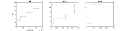
Figure 1: Search rank of SDPF for the instance $n=1000$ in Table 3 with different rank increasing parameter $\tau.$

Table 3: Comparison of SDPF and QSDPNAL for sensor network localization SDP. The rank reported is the numerical rank of the output $R$ of SDPF.

problem	algorithm	Rp	Rd	Rc	obj	time
n = 300	SDPF	0.00e+00	4.64e-07	1.76e-09	-2.1939425e-01	7.03e+00
rank = 12	QSDPNAL	4.05e-11	6.39e-06	2.63e-04	-2.1937102e-01	1.38e+02
n = 400	SDPF	0.00e+00	3.04e-07	6.66e-09	-2.1655246e-01	5.58e+00
rank = 13	QSDPNAL	3.93e-11	3.38e-07	3.55e-04	-2.1651659e-01	2.29e+02
n = 500	SDPF	0.00e+00	1.24e-07	2.82e-08	-2.1084873e-01	9.70e+00
rank = 15	QSDPNAL	4.43e-11	2.24e-06	1.29e-04	-2.1075949e-01	4.62e+02
n = 1000	SDPF	0.00e+00	3.12e-07	7.38e-09	-2.1248491e-01	2.83e+01
rank = 17	QSDPNAL	-	-	-	-	-
n = 2000	SDPF	0.00e+00	5.32e-07	4.93e-08	-2.0585246e-01	7.25e+01
rank = 23	QSDPNAL	-	-	-	-	-
n = 3000	SDPF	0.00e+00	8.87e-07	2.12e-08	-2.0396304e-01	1.21e+02
rank = 23	QSDPNAL	-	-	-	-	-
n = 5000	SDPF	0.00e+00	7.45e-07	8.56e-09	-1.8536891e-01	2.93e+02
rank = 23	QSDPNAL	-	-	-	-	-
n = 10000	SDPF	0.00e+00	6.51e-07	3.07e-08	-1.5063329e-01	6.79e+02
rank = 23	QSDPNAL	-	-	-	-	-

From Table 3, we can see that SDPF can solve all the problems to the required accuracy and it is much more efficient than QSDPNAL. The rank of every optimal solution is greater than $r_{0}=3,$ but our rank-adaptive method can progressively increase the rank and converge to the global optimal solution. Figure 1 shows the rank updating process for different increasing rank parameter $\tau$.

6.3 Box-constrained quadratic programming

Vandenbussche and Nemhauser considered the following box-constrained quadratic programming problem in [50]:

$$\min\left\{\frac{1}{2}z^{\top}Qz+a^{\top}z:\ 0\leq z\leq e,\ z\in\mathbb{R}^{n}\right\},$$ (96)

where $Q\in\mathbb{S}^{n},$ $a\in\mathbb{R}^{n}$ are given data. We consider its SDP relaxation below:

$$\min\left\{\frac{1}{2}\big{\langle}Q,Z\big{\rangle}+a^{\top}z:\ {\rm diag}(Z)+x=z,\ X:=\begin{pmatrix}1&z^{\top}\\ z&Z\end{pmatrix}\in\mathbb{S}^{n+1}_{+},\ x\in\mathbb{R}^{n}_{+}\right\}.$$ (97)

Observe that (97) has the form of (SDP) with $k=1.$ We generate the data $Q$ and $a$ following the procedure mentioned in Section 4 of [50].

Table 4: Comparison of SDPF, SDPNAL and SDPLR for SDP relaxation of box-constrained QP. In the table, $\rho$ is the density of $Q.$

problem	algorithm	Rp/Rd/Rc	obj	time	${\rm T}_{\rm alg}$/${\rm T}_{\rm cg}$/${\rm T}_{\rm lin}$/${\rm T}_{\rm ch}$
n = 1000	SDPF	3.2e-09/1.5e-07/9.0e-09	-1.4909488e+05	1.59e+00	186/362/362/
$\rho$ = 2.50e-01	SDPNAL	2.5e-07/2.3e-08/1.3e-04	-1.4909487e+05	1.10e+03	7301/2769/501/
	SDPLR	8.3e-07/2.8e-06/7.3e-06	-1.4909507e+05	3.08e+01	18/8979/-/
n = 1000	SDPF	4.3e-12/4.3e-08/2.1e-08	-2.5806628e+05	1.50e+00	184/353/353/
$\rho$ = 7.50e-01	SDPNAL	4.1e-07/4.1e-07/6.1e-05	- 2.5806644e+05	9.53e+02	5688/2848/488/
	SDPLR	9.4e-07/2.2e-06/7.3e-06	-2.5806657e+05	1.87e+01	19/5283/-/
n = 2000	SDPF	5.8e-09/4.1e-08/1.4e-07	-4.3135148e+05	3.81e+00	185/372/372/
$\rho$ = 2.50e-01	SDPNAL	-	-	-	-
	SDPLR	9.9e-07/7.1e-07/3.4e-05	-4.3135227e+05	4.76e+02	18/21690/-/
n = 2000	SDPF	2.7e-11/8.2e-08/9.3e-08	-7.5485516e+05	4.19e+00	261/506/506/
$\rho$ = 7.50e-01	SDPNAL	-	-	-	-
	SDPLR	9.6e-07/6.0e-07/1.0e-04	-7.5485379e+05	3.86e+02	20/17561/-/
n = 5000	SDPF	1.2e-09/4.6e-08/1.2e-08	-1.7227960e+06	1.96e+01	352/663/663/
$\rho$ = 2.50e-01	SDPNAL	-	-	-	-
	SDPLR	2.9e-05/1.0e-06/6.3e-04	-1.7228807e+06	3.61e+03	18/25940/-/
n = 5000	SDPF	2.3e-10/1.2e-08/3.7e-07	-3.0025339e+06	1.97e+01	317/624/624/
$\rho$ = 7.50e-01	SDPNAL	-	-	-	-
	SDPLR	5.2e-06/3.7e-06/2.2e-03	-3.0025039e+06	3.61e+03	18/25380/-/
n = 10000	SDPF	6.6e-10/2.0e-08/2.8e-07	-4.8841142e+06	9.46e+01	567/1036/1036/
$\rho$ = 2.50e-01	SDPNAL	-	-	-	-
	SDPLR	-	-	-	-
n = 10000	SDPF	6.7e-09/1.4e-08/1.9e-08	-8.4655873e+06	1.08e+02	729/1266/1266/
$\rho$ = 7.50e-01	SDPNAL	-	-	-	-
	SDPLR	-	-	-	-

From Table 4, we can see that SDPF is significantly faster than SDPLR and SDPNAL. For some instances, SDPF can be more than 100 times faster than SDPLR and nearly 1000 times faster than SDPNAL. Moreover, SDPF can solve all the problems more accurately than SDPLR and SDPNAL. The feasible set of (SDPR) is the Cartesian product of unit spheres, i.e., an oblique manifold. In this case, the coefficient matrix $Q_{i}$ of the linear system in the projection and retraction mapping is diagonal. As mentioned in subsection 4, we use ${\rm Diag}(Q_{i})^{-1}=Q_{i}^{-1}$ to be the preconditioner before the random perturbation. Thus, our PCG converges in one iteration, which explains why ${\rm T}_{\rm cg}={\rm T}_{\rm lin}$ for SDPF. Without dealing with the constraint $X_{11}=1$ as in (SDPR) explicitly, the Jacobian matrix of the constraints can be ill-conditioned, which results in the large number of iterations ${\rm T}_{\rm cg}$ for SDPLR to solve the ALM subproblems. This demonstrates the effectiveness of our model (SDPR) as compared to the traditional BM factorization.

6.4 The Lovász Theta SDP

The problems we have tested before are mostly nondegenerate. In order to verify the effectiveness of our random perturbation strategy, we test the following Lovász Theta SDP problem [38] and frequently used as benchmarks for SDP solvers:

$$\min\left\{-\big{\langle}ee^{\top},X\big{\rangle}:\ \big{\langle}I,X\big{\rangle}=1,\ \mathcal{A}_{G}\left(X\right)=0,\ X\in\mathbb{S}^{n}_{+}\right\},$$ (98)

where $G=(V,E)$ is a simple undirected graph, $\mathcal{A}_{G}:\mathbb{S}^{n}\rightarrow\mathbb{R}^{m}$ is defined by $\mathcal{A}_{G}(X):=\left(X_{ij}\right)_{ij\in E}.$ We consider two types of graphs in our experiments. The first type of graph, which contains fewer than 3000 vertices, comes from coding theory [43]. Such a dataset has already been tested in [61], where SDPNAL achieves good performance. The second group of graphs are large sparse graphs coming from Gset such that $n\geq 5000.$ Note that some of the Gset graphs such as g58 and g59 have the same structure with the only difference in the edge weight. We only show the result of one of those graphs. All the problems we test are degenerate, so we apply our random perturbation strategy mentioned in subsection 4.2. The KKT residue reported in the following tables is for the original unperturbed problem. Our random perturbation is kept to be sufficiently small so that the primal residue of the output of SDPF can reach the required accuracy of $10^{-6}.$ For some extremely ill-conditioned problems such as g58 and g63, we add a larger perturbation and set the tolerance to be $10^{-5}.$ Apart from the random perturbation, we also apply the dual refinement in Section 5 to improve the dual KKT residue of the output. The time spent in the dual refinement is part of the running time.

Table 5: Comparison of SDPF, SDPNAL and SDPLR for Lovász Theta SDP in coding theory. In the first column, $n=|V|$ and $m=|E|.$

problem	algorithm	Rp/Rd/Rc	obj	time	${\rm T}_{\rm alg}$/${\rm T}_{\rm cg}$/${\rm T}_{\rm lin}$/${\rm T}_{\rm ch}$
1dc.1024	SDPF	7.5e-07/3.8e-07/7.9e-07	-9.5991877e+01	5.85e+02	598/25788/1012/9
n = 1024	SDPNAL	6.5e-07/6.6e-07/2.9e-08	-9.5986248e+01	1.02e+02	251/5165/51/-
m = 24063	SDPLR	1.0e-06/1.3e-06/2.6e-08	-9.5987268e+01	8.68e+02	19/87756/-/-
1dc.2048	SDPF	7.5e-07/2.3e-07/4.8e-06	-1.7474015e+02	1.68e+03	428/19948/671/42
n = 2048	SDPNAL	3.7e-07/3.0e-07/5.8e-09	-1.7473095e+02	8.07e+02	273/8668/73/-
m = 58367	SDPLR	-	-	-	-
1et.1024	SDPF	7.6e-07/6.6e-07/8.1e-07	-1.8423771e+02	4.92e+01	176/3045/265/9
n = 1024	SDPNAL	4.3e-07/4.6e-07/4.9e-09	-1.8422716e+02	7.81e+02	4167/18570/167/-
m = 9600	SDPLR	1.0e-06/5.5e-06/9.6e-09	-1.8423119e+02	1.85e+03	19/257078/-/-
1et.2048	SDPF	7.6e-07/8.5e-07/2.3e-07	-3.4206073e+02	1.50e+02	218/4998/324/4
n = 2048	SDPNAL	2.0e-07/3.2e-07/3.6e-08	-3.4202941e+02	2.39e+03	714/26604/214/-
m = 22528	SDPLR	9.7e-04/8.2e-04/2.9e-05	-3.5833285e+02	3.60e+03	14/87907/-/-
1tc.1024	SDPF	7.5e-07/5.4e-07/2.6e-07	-2.0631684e+02	6.32e+01	190/2914/312/16
n = 1024	SDPNAL	7.0e-07/3.8e-07/1.4e-08	-2.0630546e+02	5.45e+02	1615/26745/229/-
m = 7936	SDPLR	1.0e-06/5.2e-06/4.1e-07	-2.0630913e+02	1.18e+03	18/182339/-/-
1tc.2048	SDPF	7.6e-07/5.1e-07/7.0e-07	-3.7467663e+02	1.78e+02	224/6520/324/8
n = 2048	SDPNAL	8.5e-07/2.6e-07/5.6e-07	-3.7464643e+02	2.75e+03	1188/30071/269/-
m = 18944	SDPLR	1.5e-05/4.1e-04/2.4e-04	-3.7486924e+02	3.60e+03	15/91296/-/-
1zc.1024	SDPF	7.5e-07/8.5e-07/4.6e-07	-1.2867552e+02	2.96e+02	430/18411/592/106
n = 1024	SDPNAL	6.3e-08/1.5e-07/7.6e-11	-1.2866668e+02	4.26e+01	217/710/17/-
m = 16640	SDPLR	1.0e-06/8.8e-08/3.0e-09	-1.2866796e+02	2.70e+03	18/322387/-/-
1zc.2048	SDPF	7.6e-07/5.0e-07/1.6e-08	-2.3742455e+02	1.24e+02	85/2661/124/3
n = 2048	SDPNAL	5.4e-08/3.8e-09/7.8e-11	-2.3739996e+02	4.01e+02	233/1607/33/-
m = 39424	SDPLR	9.3e-04/1.8e-05/5.2e-07	-2.4748487e+02	3.60e+03	16/69904/-/-

Table 6: Test SDPF for Lovász Theta SDP in Gset. $n,m$ denotes the number of vertices and edges respectively.

problem: $n,m$	Rp/Rd/Rc	obj	time	${\rm T}_{\rm alg}$/${\rm T}_{\rm cg}$/${\rm T}_{\rm lin}$/${\rm T}_{\rm ch}$
g55: 5000,12498	7.5e-07/8.1e-07/1.5e-07	-2.3243020e+03	7.96e+01	231/3824/262/3
g57: 5000,10000	7.0e-09/1.7e-07/8.5e-11	-2.4999998e+03	3.96e+01	355/4162/582/36
g58: 5000,29570	7.5e-06/9.4e-06/7.0e-07	-1.7833429e+03	6.68e+02	219/10369/326/93
g60: 7000,17148	7.5e-07/6.7e-07/2.7e-07	-3.2652524e+03	1.73e+02	245/4809/359/3
g62: 7000,14000	2.2e-08/1.5e-07/2.6e-10	-3.4999998e+03	5.61e+01	259/4138/467/16
g63: 7000,41459	7.5e-06/6.9e-06/3.3e-07	-2.4946356e+03	1.02e+03	160/6174/238/32
g65: 8000,16000	7.5e-10/0.0e+00/2.8e-07	-3.9999992e+03	9.98e+01	490/6450/800/65
g66: 9000,18000	1.4e-08/2.0e-07/9.6e-12	-4.4999995e+03	8.23e+01	404/4630/641/56
g67: 10000,20000	6.0e-09/0.0e+00/1.2e-07	-4.9999992e+03	1.19e+02	342/4156/539/25
g70: 10000,9999	7.6e-07/8.8e-07/3.0e-08	-6.0777626e+03	7.12e+02	158/3686/224/13
g77: 14000,28000	7.1e-09/5.8e-07/1.9e-10	-6.9999967e+03	2.06e+02	542/7009/932/60
g81: 20000,40000	3.4e-09/6.0e-14/3.5e-08	-1.0000000e+04	6.37e+02	1038/10142/1594/94

From Table 5, we can see that SDPF can solve most of the instances to the required accuracy $10^{-6}.$ For those instances that SDPF didn’t reach the tolerance, the KKT residues are already close to $10^{-6}.$ This verifies the robustness of SDPF. As for the speed, both SDPF and SDPNAL are faster than SDPLR but there is no clear winner between SDPF and SDPNAL. Actually, SDPF can be either ten times faster than SDPNAL (1et.2048, 1tc.2048) or nearly 7 times slower than SDPNAL (1zc.1024). This is in line with our expectation because $n$ is moderate and the degeneracy is not significant for this dataset. However, when we test the large sparse Gset graphs that are highly degenerate, we find that neither SDPNAL nor SDPLR can solve any of the instances up to even low accuracy. Thus, we only show the results for SDPF. From Table 6, we can see that SDPF can solve all the problems to the required accuracy. Note that for g58 and g63, we have increased the tolerance to be $10^{-5}$ due to the extreme ill-conditioning. In Algorithm 1, the number of Cholesky decompositions is usually at least ten times smaller than the number of linear systems solved in Algorithm 1. Besides, the PCG iterations for Algorithm 1 is much smaller than the number of subiterations for SDPLR. This demonstrates the effectiveness of our random perturbation and dual refinement strategies. For the largest graph g81 with 20000 vertices, SDPF can find the solution within 11 minutes. This demonstrates the efficiency of our algorithm for solving large scale low-rank SDP problems.

7 Conclusion

In this paper, we propose a rank-support adaptive feasible method to solve general convex SDP problems with guaranteed convergence. We apply random perturbation and dual refinement strategies to overcome the numerical difficulty caused by the issue of degeneracy. Our work have significantly extended the application range of feasible method for solving convex SDP problems.

References

• [1] P.-A. Absil, R. Mahony, and R. Sepulchre. Optimization algorithms on matrix manifolds. In Optimization Algorithms on Matrix Manifolds. Princeton University Press, 2009.
• [2] P.-A. Absil and J. Malick. Projection-like retractions on matrix manifolds. SIAM J. Optimization, 22(1):135–158, 2012.
• [3] F. Alizadeh, J.-P. A. Haeberly, and M. L. Overton. Complementarity and nondegeneracy in semidefinite programming. Mathematical Programming, 77(1):111–128, 1997.
• [4] K. M. Anstreicher. Semidefinite programming versus the reformulation-linearization technique for nonconvex quadratically constrained quadratic programming. J. of Global Optimization, 43(2):471–484, 2009.
• [5] M. ApS. Mosek optimization toolbox for matlab. User’s Guide and Reference Manual, Version, 4, 2019.
• [6] Y. Bai, J. Duchi, and S. Mei. Proximal algorithms for constrained composite optimization, with applications to solving low-rank sdps. arXiv preprint arXiv:1903.00184, 2019.
• [7] A. S. Bandeira, N. Boumal, and V. Voroninski. On the low-rank approach for semidefinite programs arising in synchronization and community detection. In Conference on Learning Theory, pages 361–382. PMLR, 2016.
• [8] A. I. Barvinok. Problems of distance geometry and convex properties of quadratic maps. Discrete & Computational Geometry, 13(2):189–202, 1995.
• [9] S. Bellavia, J. Gondzio, and M. Porcelli. A relaxed interior point method for low-rank semidefinite programming problems with applications to matrix completion. Journal of Scientific Computing, 89(2):46, 2021.
• [10] S. Bhojanapalli, N. Boumal, P. Jain, and P. Netrapalli. Smoothed analysis for low-rank solutions to semidefinite programs in quadratic penalty form. In Conference On Learning Theory, pages 3243–3270. PMLR, 2018.
• [11] P. Biswas, T.-C. Liang, K.-C. Toh, Y. Ye, and T.-C. Wang. Semidefinite programming approaches for sensor network localization with noisy distance measurements. IEEE Transactions on Automation Science and Engineering, 3(4):360–371, 2006.
• [12] J. F. Bonnans and A. Shapiro. Perturbation analysis of optimization problems. Springer Science & Business Media, 2013.
• [13] N. Boumal. A Riemannian low-rank method for optimization over semidefinite matrices with block-diagonal constraints. arXiv preprint arXiv:1506.00575, 2015.
• [14] N. Boumal. An introduction to optimization on smooth manifolds. Available online, May, 3, 2020.
• [15] N. Boumal, P.-A. Absil, and C. Cartis. Global rates of convergence for nonconvex optimization on manifolds. IMA J. of Numerical Analysis, 39(1):1–33, 2019.
• [16] N. Boumal, B. Mishra, P.-A. Absil, and R. Sepulchre. Manopt, a Matlab toolbox for optimization on manifolds. J. of Machine Learning Research, 15(1):1455–1459, 2014.
• [17] N. Boumal, V. Voroninski, and A. Bandeira. The non-convex Burer-Monteiro approach works on smooth semidefinite programs. Advances in Neural Information Processing Systems, 29, 2016.
• [18] N. Boumal, V. Voroninski, and A. S. Bandeira. Deterministic guarantees for Burer-Monteiro factorizations of smooth semidefinite programs. Communications on Pure and Applied Mathematics, 73(3):581–608, 2020.
• [19] S. Burer and C. Choi. Computational enhancements in low-rank semidefinite programming. Optimisation Methods and Software, 21(3):493–512, 2006.
• [20] S. Burer and R. D. Monteiro. A nonlinear programming algorithm for solving semidefinite programs via low-rank factorization. Mathematical Programming, 95(2):329–357, 2003.
• [21] S. Burer and R. D. Monteiro. Local minima and convergence in low-rank semidefinite programming. Mathematical Programming, 103(3):427–444, 2005.
• [22] Z. X. Chan and D. Sun. Constraint nondegeneracy, strong regularity, and nonsingularity in semidefinite programming. SIAM J. Optimization, 19(1):370–396, 2008.
• [23] D. Cifuentes. On the Burer–Monteiro method for general semidefinite programs. Optimization Letters, 15(6):2299–2309, 2021.
• [24] M. A. Erdogdu, A. Ozdaglar, P. A. Parrilo, and N. D. Vanli. Convergence rate of block-coordinate maximization Burer–Monteiro method for solving large SDPs. Mathematical Programming, 195(1-2):243–281, 2022.
• [25] S. Friedland and R. Loewy. Subspaces of symmetric matrices containing matrices with a multiple first eigenvalue. Pacific J. of Mathematics, 62(2):389–399, 1976.
• [26] B. Gao and P.-A. Absil. A Riemannian rank-adaptive method for low-rank matrix completion. Computational Optimization and Applications, 81(1):67–90, 2022.
• [27] B. Gao, N. T. Son, P.-A. Absil, and T. Stykel. Riemannian optimization on the symplectic Stiefel manifold. SIAM J. Optimization, 31(2):1546–1575, 2021.
• [28] R. Ge, C. Jin, and Y. Zheng. No spurious local minima in nonconvex low rank problems: A unified geometric analysis. In International Conference on Machine Learning, pages 1233–1242. PMLR, 2017.
• [29] M. W. Hirsch. Differential topology, volume 33. Springer Science & Business Media, 2012.
• [30] B. Iannazzo and M. Porcelli. The Riemannian Barzilai–Borwein method with nonmonotone line search and the matrix geometric mean computation. IMA J. of Numerical Analysis, 38(1):495–517, 2018.
• [31] M. Journée, F. Bach, P.-A. Absil, and R. Sepulchre. Low-rank optimization on the cone of positive semidefinite matrices. SIAM J. Optimization, 20(5):2327–2351, 2010.
• [32] H. Karimi, J. Nutini, and M. Schmidt. Linear convergence of gradient and proximal-gradient methods under the Polyak-Lojasiewicz condition. In Machine Learning and Knowledge Discovery in Databases: European Conference, ECML PKDD 2016, Riva del Garda, Italy, September 19-23, 2016, Proceedings, Part I 16, pages 795–811. Springer, 2016.
• [33] M. Kochurov, R. Karimov, and S. Kozlukov. Geoopt: Riemannian optimization in pytorch. arXiv preprint arXiv:2005.02819, 2020.
• [34] C.-p. Lee, L. Liang, T. Tang, and K.-C. Toh. Accelerating nuclear-norm regularized low-rank matrix optimization through Burer-Monteiro decomposition. arXiv preprint arXiv:2204.14067, 2022.
• [35] X. Li, D. Sun, and K.-C. Toh. QSDPNAL: a two-phase augmented Lagrangian method for convex quadratic semidefinite programming. Mathematical Programming Computation, 10(4):703–743, 2018.
• [36] S. Lojasiewicz. A topological property of real analytic subsets. Coll. du CNRS, Les équations aux dérivées partielles, 117(87-89):2, 1963.
• [37] B. F. Lourenço, E. H. Fukuda, and M. Fukushima. Optimality conditions for nonlinear semidefinite programming via squared slack variables. Mathematical Programming, 168:177–200, 2018.
• [38] L. Lovász. On the Shannon capacity of a graph. IEEE Transactions on Information theory, 25(1):1–7, 1979.
• [39] J. Malick, J. Povh, F. Rendl, and A. Wiegele. Regularization methods for semidefinite programming. SIAM J. Optimization, 20(1):336–356, 2009.
• [40] G. Pataki. On the rank of extreme matrices in semidefinite programs and the multiplicity of optimal eigenvalues. Mathematics of Operations Research, 23(2):339–358, 1998.
• [41] T. Pumir, S. Jelassi, and N. Boumal. Smoothed analysis of the low-rank approach for smooth semidefinite programs. Advances in Neural Information Processing Systems, 31, 2018.
• [42] S. Scholtes and M. Stöhr. How stringent is the linear independence assumption for mathematical programs with complementarity constraints? Mathematics of Operations Research, 26(4):851–863, 2001.
• [43] N. J. A. Sloane. Challenge problems: Independent sets in graphs. http://www. research. att. com/~ njas/doc/graphs. html, 2005.
• [44] D. Sun, K.-C. Toh, Y. Yuan, and X.-Y. Zhao. SDPNAL+: A Matlab software for semidefinite programming with bound constraints (version 1.0). Optimization Methods and Software, 35(1):87–115, 2020.
• [45] T. Tang and K.-C. Toh. Solving graph equipartition SDPs on an algebraic variety. arXiv preprint arXiv:2112.04256, 2021.
• [46] T. Tang and K.-C. Toh. A feasible method for solving an SDP relaxation of the quadratic knapsack problem. Mathematics of Operations Research, to appear, 2023.
• [47] K.-C. Toh, M. J. Todd, and R. H. Tütüncü. SDPT3—a Matlab software package for semidefinite programming, version 1.3. Optimization Methods and Software, 11(1-4):545–581, 1999.
• [48] R. H. Tütüncü, K.-C. Toh, and M. J. Todd. Solving semidefinite-quadratic-linear programs using SDPT3. Mathematical Programming, 95(2):189–217, 2003.
• [49] A. Uschmajew and B. Vandereycken. Greedy rank updates combined with Riemannian descent methods for low-rank optimization. In International Conference on Sampling Theory and Applications (SampTA), pages 420–424. IEEE, 2015.
• [50] D. Vandenbussche and G. L. Nemhauser. A branch-and-cut algorithm for nonconvex quadratic programs with box constraints. Mathematical Programming, 102(3):559–575, 2005.
• [51] J. Wang and L. Hu. Solving low-rank semidefinite programs via manifold optimization. arXiv preprint arXiv:2303.01722v1, 2023.
• [52] Y. Wang, K. Deng, H. Liu, and Z. Wen. A decomposition augmented lagrangian method for low-rank semidefinite programming. SIAM Journal on Optimization, 33(3):1361–1390, 2023.
• [53] Z. Wen and W. Yin. A feasible method for optimization with orthogonality constraints. Mathematical Programming, 142(1):397–434, 2013.
• [54] N. Xiao, X. Hu, X. Liu, and K.-C. Toh. Cdopt: A python package for a class of Riemannian optimization. arXiv preprint arXiv:2212.02698, 2022.
• [55] N. Xiao, X. Liu, and K.-C. Toh. Constraint dissolving approaches for Riemannian optimization. arXiv preprint arXiv:2203.10319, 2022.
• [56] L. Yang, D. Sun, and K.-C. Toh. SDPNAL+: a majorized semismooth Newton-CG augmented Lagrangian method for semidefinite programming with nonnegative constraints. Mathematical Programming Computation, 7(3):331–366, 2015.
• [57] A. Yurtsever, J. A. Tropp, O. Fercoq, M. Udell, and V. Cevher. Scalable semidefinite programming. SIAM J. on Mathematics of Data Science, 3(1):171–200, 2021.
• [58] J. Zhang, S. Fattahi, and R. Y. Zhang. Preconditioned gradient descent for over-parameterized nonconvex matrix factorization. Advances in Neural Information Processing Systems, 34:5985–5996, 2021.
• [59] R. Zhang. Newton retraction as approximate geodesics on submanifolds. arXiv preprint arXiv:2006.14751, 2020.
• [60] R. Y. Zhang. Improved global guarantees for the nonconvex burer–monteiro factorization via rank overparameterization. arXiv preprint arXiv:2207.01789, 2022.
• [61] X.-Y. Zhao, D. Sun, and K.-C. Toh. A Newton-CG augmented Lagrangian method for semidefinite programming. SIAM J. Optimization, 20(4):1737–1765, 2010.
• [62] G. Zhou, W. Huang, K. A. Gallivan, P. Van Dooren, and P.-A. Absil. A Riemannian rank-adaptive method for low-rank optimization. Neurocomputing, 192:72–80, 2016.