Universal Incomplete-View CT Reconstruction with
Prompted Contextual Transformer

Abstract

Despite the reduced radiation dose, suitability for objects with physical constraints, and accelerated scanning procedure, incomplete-view computed tomography (CT) images suffer from severe artifacts, hampering their value for clinical diagnosis. The incomplete-view CT can be divided into two scenarios depending on the sampling of projection, sparse-view CT and limited-angle CT, each encompassing various settings for different clinical requirements. Existing methods tackle with these settings separately and individually due to their significantly different artifact patterns; this, however, gives rise to high computational and storage costs, hindering its flexible adaptation to new settings. To address this challenge, we present the first-of-its-kind all-in-one incomplete-view CT reconstruction model with PROmpted Contextual Transformer, termed ProCT. More specifically, we first devise the projection view-aware prompting to provide setting-discriminative information, enabling a single model to handle diverse incomplete-view CT settings. Then, we propose artifact-aware contextual learning to provide the contextual guidance of image pairs from either CT phantom or publicly available datasets, making ProCT capable of accurately removing the complex artifacts from the incomplete-view CT images. Extensive experiments demonstrate that ProCT can achieve superior performance on a wide range of incomplete-view CT settings using a single model. Remarkably, our model with only image-domain information surpasses the state-of-the-art dual-domain methods that require the access to raw data. The code is available at: https://github.com/Masaaki-75/proct

Abstract

This supplementary material includes five parts: (A) network architecture, (B) detailed experimental setup, (C) more ablation studies, (D) more visualization examples, and (E) limitation.

1 Introduction

X-ray computed tomography (CT) is a cornerstone in the field of medical imaging, providing valuable insights into the internal structures of human body non-invasively. This technique acquires x-ray raw data (a.k.a. projection data, or sinogram) from different views around the subject, which are then used to reconstruct detailed cross-sectional images [26]. Despite the benefits, conventional CT imaging acquires a full set of raw data from various views, leading to increased radiation dose and prolonged scanning time. Moreover, there might be patients with specific anatomical restriction that makes a full-view scan impractical.

Incomplete-view CT has emerged as a promising solution to reducing the radiation dose, accelerated scanning time [5], and accommodating physical constraints or irregular scenarios in medical imaging [1, 19], which only acquires a small set of projection data. This strategy can be further categorized as sparse-view CT (SVCT) and limited-angle CT (LACT), depending on different sampling patterns shown in Fig. 1. Concretely, for the fan-beam CT, typical SVCT setting samples projection from equidistant views covering $[0^{\circ},360^{\circ}]$. On the other hand, LACT selects projections from views that cover a specific range of angles. Both SVCT and LACT result in a fairly small number of views compared to the pre-determined full-view number.

In either case, there exists a range of settings tailored to specific clinical requisites, and the incomplete raw data can lead to distinct artifacts globally distributed on the image reconstructed by conventional filtered back-projection (FBP) algorithms [25]. Existing methods handle these settings in isolation, requiring the training of a separate model for each setting. However, this “one-model-for-one-setting” fashion not only results in increased training efforts and storage overhead, but also yields inflexible single-setting models with limited adaptability to alternative clinical settings.

Another issue arises within each specific setting. Dominant dual-domain methods [24, 6, 13] have shown superior in restoring a high-quality CT image by using knowledge from both sinogram and image domains. Unfortunately, the required sinogram is often inaccessible due to commercial privacy concerns, compromising the efficacy of these methods. Moreover, dual-domain methods can underperform the image-domain ones when the sinogram is extremely sparse, due to the increased error of sinogram completion [10, 11]. This dual challenge of handling settings separately and the inherent limitation of dual-domain learning underscores the need for a unified and adaptable image-domain method in incomplete-view CT reconstruction.

To this end, we present PROmpted Contextual Transformer (ProCT), an all-in-one image-domain model to perform universal CT reconstruction across diverse incomplete-view CT settings, as depicted in Fig. 1. The novelties of our ProCT are two-fold. First, to empower ProCT with the reconstruction ability on a wide range of fine-grained incomplete-view settings, we propose the view-aware prompting technique to inject the setting-discriminative information into the network. Second, to capture the complex artifact pattern within each setting given no sinogram data, we propose artifact-aware contextual learning that leverages the contextual information from another incomplete- and full-view CT image pair to remove the artifact in the input incomplete-view CT image. In doing so, ProCT can achieve universal incomplete-view CT reconstruction without access to the raw data, and outperform the state-of-the-art methods, including those using raw data.

In summary, our contributions are as follows:

• We present a prompted contextual transformer or ProCT for universal incomplete-view CT reconstruction. To the best of our knowledge, this is the first to address the challenging universal task with diverse settings, using a single one-pass model with only image-domain data.

• We propose view-aware prompting to provide setting-discriminative knowledge, which endows ProCT with the capability to handle a wide range of incomplete-view CT images within a single model.

• We propose artifact-aware contextual learning to sense the artifact pattern information from an incomplete- and full-view CT phantom pair, which can ensure a better grasp of the artifacts without the sinogram data.

• Extensive experimental results demonstrate the superiority of ProCT over state-of-the-art reconstruction methods across diverse incomplete-view CT scenarios and settings. Remarkably, our ProCT is a single model to handle all settings compared to existing methods that require different models for different settings.

2 Related Work

Learning-based incomplete-view CT reconstruction.

Existing learning-based methods for incomplete-view CT reconstruction mainly include image-domain methods and dual-domain ones. Image-domain methods [7, 32, 11] takes the incomplete-view CT images as input and treat the reconstruction as an image post-processing task. On the other hand, dual-domain methods utilizes both the incomplete-view sinogram data and image data.

Generally, dual-domain methods excel in accurately restoring incomplete-view CT images compared to simple image-domain methods, as they leverage information from two domains. Some approaches [31, 30] unroll the conventional iterative algorithms into deep learning frameworks, others [24, 6, 13] perform sinogram in-painting and image post-processing simultaneously.

Unfortunately, these methods are designed in a single-setting manner and lack transferability and flexibility, requiring re-training once the clinical practice opts to a new CT scenario or setting. Also, the state-of-the-art methods are dual-domain and cannot avoid the inherent limitations mentioned in Sec. 1. Shu et al. [20] proposed to use deep image prior [22] to tackle SVCT and LACT with one model. However, their method is computationally intensive, needing hundreds of iterations to process every single image.

Unlike existing work, our model addresses the universal incomplete-view CT reconstruction task with fine-grained settings in one pass, using only image-domain data.

Universal models for image restoration.

Inspired by the remarkable generalizability of large language models and generation models, recent research has turned to resolving various tasks [23] in the field of image restoration. Notably, prompt-based methods and in-context learning have shown their great potential. Prompt-based methods aim to condition the inputs by task-related knowledge without altering the model parameters, offering great flexibility. Pioneering work such as PromptIR [17] and RroRes [14] utilize prompts for universal image restoration and demonstrate their effectiveness in low-level vision. In-context learning [3], on the other hand, aims to teach the model to imitate the given example and improve the generalizability in a few-shot fashion. For example, MAE-VQGAN [2] and Painter [27] can reason on the query input guided by contextual input-output examples, thereby performing various visual tasks using a single model.

In contrast, we propose incorporating the view-aware prompting technique and artifact-aware contextual learning for universal incomplete-view CT reconstruction, where the view prompt encodes the semantic of the incomplete-view CT sampling view distribution, and contextual learning provides the complementary image-domain information for better grasping the complex artifact patterns.

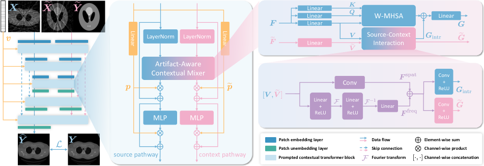
Figure 2: Overview of the proposed ProCT. Detailed configurations can be found in Sec. A in our supplementary material.

3 Method

3.1 Problem formulation and motivation

Typical CT scanning produces a series of x-ray sinogram data (a.k.a. raw data) as an object is rotated within a scanner. The full-view sinogram, $\boldsymbol{S}\in\mathbb{R}^{{N^{\mathrm{full}}_{\mathrm{view}}}\times{N_{\mathrm{det}}}}$, represents the attenuation of x-rays through the object from various views, where ${N^{\mathrm{full}}_{\mathrm{view}}}$ denotes the number of full views and ${N_{\mathrm{det}}}$ the number of detectors. Through back-projection algorithm $\mathcal{B}$ (e.g., FBP), $\boldsymbol{S}$ can be used to reconstruct a CT image $\boldsymbol{Y}=\mathcal{B}(\boldsymbol{S})$ visualizing the inner structures in the object.

As shown in Fig. 1, in the incomplete-view CT scenarios, we only sample a small portion of the full-view sinogram $\boldsymbol{S}$ for imaging, which can reduce the radiation dose and accommodate physical restrictions. Concretely, we use a view sampling vector $\boldsymbol{v}\in\{0,1\}^{{N^{\mathrm{full}}_{\mathrm{view}}}}$ to decide which projection views are sampled from $\boldsymbol{S}$, i.e., the $1$ values in $\boldsymbol{v}$ indicate the view distribution. For SVCT, the values are equidistantly distributed, while for LACT, they are localized on a contiguous segment. With $\boldsymbol{v}$, we can create the incomplete-view sinogram, $\boldsymbol{S}_{\text{in}}=\mathcal{R}(\mathrm{diag}(\boldsymbol{v})\cdot\boldsymbol{S})$, where $\mathcal{R}$ is a reduction operator to remove the zero rows, and $\boldsymbol{S}_{\text{in}}\in\mathbb{R}^{{N_{\mathrm{view}}}\times{N_{\mathrm{det}}}}$ has fewer valid views (i.e., ${N_{\mathrm{view}}}<{N^{\mathrm{full}}_{\mathrm{view}}}$).

The back-projection is then performed to produce the incomplete-view CT image $\boldsymbol{X}=\mathcal{B}(\boldsymbol{S}_{\text{in}})$. Unfortunately, this becomes an undetermined problem when ${N_{\mathrm{view}}}\ll{N^{\mathrm{full}}_{\mathrm{view}}}$, and the resulted image $\boldsymbol{X}$ presents severe and distinct artifacts given different sampling vector $\boldsymbol{v}$. The goal of incomplete-view CT reconstruction is to produce an image $\widehat{\boldsymbol{Y}}$ from $\boldsymbol{X}$ with a level of quality close to the ground-truth full-view image $\boldsymbol{Y}$.

Existing methods typically address the SVCT and LACT separately due to their distinct artifact patterns resulting from different sampling view distribution, which lacks the transferability to diverse clinical CT settings and creates an unnecessary drain on computing resources. In addition, current state-of-the-art methods use both incomplete sinogram $\boldsymbol{S}_{\text{in}}$ and the incomplete-view image $\boldsymbol{X}$ to predict $\boldsymbol{Y}$, known as dual-domain methods. However, their efficacy is hindered by the frequent unavailability of sinogram data.

Therefore, we are motivated to build a single model to achieve universal incomplete-view CT reconstruction with only image-domain data.

3.2 Overview of ProCT

Fig. 2 depicts the overall hourglass architecture of our proposed model, ProCT, consisting of several prompted contextual transformer blocks with a source pathway and a context pathway. ProCT incorporates two key designs: view-aware prompting and artifact-aware contextual learning.

View-aware prompting is crucial to achieving universal incomplete-view CT reconstruction, using a view prompt $\boldsymbol{p}$ to inject the setting-discriminative information into the model. However, $\boldsymbol{p}$ only indicates the location of artifacts, and it is still difficult to learn the complex artifact patterns without using sinogram data. Therefore, we further propose artifact-aware contextual learning to leverage the complementary information of artifact patterns from an incomplete- and full-view contextual pair $\mathcal{C}$. The reconstruction process of our ProCT $\mathcal{U}_{\Theta}$ can be formulated by

$$\widehat{\boldsymbol{Y}}=\mathcal{U}_{\Theta}(\boldsymbol{X},\mathcal{C},\boldsymbol{p}),$$ (1)

where $\boldsymbol{X}$ denotes the input source incomplete-view CT image to be reconstructed, and $\mathcal{C}=[\widetilde{\boldsymbol{X}},\widetilde{\boldsymbol{Y}}]$ denote the given contextual pair. Here, $\widetilde{\boldsymbol{X}}$ and $\widetilde{\boldsymbol{Y}}$ denote the incomplete- and full-view contextual images, respectively, and $[\cdot,\cdot]$ represents the concatenation along channel dimension.

We highlight that the view prompt can either be derived from the view sampling vector or be parameterized by some learnable vectors, and the contextual pair can be created from the commonly used CT phantom or other publicly available incomplete-view CT image datasets. We choose the CT phantom as our default setting for its easy availability. In the following, we detail these two key designs.

3.3 View-aware prompting

Prompting techniques have been applied to the universal image restoration as a powerful indicator of various restoration tasks [17, 14], where each task is typically assigned with a learnable prompt that interacts with the input images or the latent features. Nonetheless, in the context of incomplete-view CT, we are dealing with a vast range of fine-grained settings (e.g., the angular range in LACT can be any reasonable sub-interval within $[0^{\circ},360^{\circ}]$), making it impractical to assign a separate prompt for each setting. Furthermore, these incomplete-view CT settings exhibit intrinsic relations (e.g., the sampling patterns of two different settings can overlap). Treating them independently may fail to capture such relations and the resulting artifact locations in the image. Is there anything that encodes such fine-grained CT settings and their intrinsic relations?

Our answer is yes. We note that the difference between these settings essentially stem from the sampling view distribution, as evident in Fig. 1, and that the sampling vector $\boldsymbol{v}$ used to create an incomplete sinogram naturally encodes this information. Therefore, we adopt $\boldsymbol{v}$ to construct our view prompt. To improve the expressivity without introducing excessive complexity, we simply apply two individual linear layers to create view prompts $\boldsymbol{p}=f_{\mathrm{lin}}^{\mathrm{src}}(\boldsymbol{v})$ and $\widetilde{\boldsymbol{p}}=f_{\mathrm{lin}}^{\mathrm{con}}(\boldsymbol{v})$ for the source and context pathways, respectively. These prompts modulate the features output from both the mixer and the multi-layer perceptron (MLP) within each transformer block. For instance, let $\boldsymbol{H}\in\mathbb{R}^{C\times L}$ denote the $C$-channel input for source pathway MLP, the MLP output $\boldsymbol{H}_{\mathrm{mlp}}\in\mathbb{R}^{C\times L}$ is modulated by $\boldsymbol{p}\in\mathbb{R}^{C}$ as follows,

$$\boldsymbol{H}_{\mathrm{mlp}} =\boldsymbol{H}+\boldsymbol{p}\otimes f_{\mathrm{mlp}}^{\mathrm{src}}(\boldsymbol{H}),$$ (2)

where $\otimes$ is the channel-wise product. The modulations elsewhere are similar, as shown in Fig. 2. We add that $\boldsymbol{v}$ can also be parameterized as a learnable vector with simple modification, and we leave this in Sec. C.1.

3.4 Artifact-aware contextual learning

View prompt encodes the semantic of view distribution and indicates the location of the artifacts. However, learning the complex artifact patterns is still challenging for our image-domain model due to the loss of sinogram information.

To address this issue, we seek help from an incomplete- and full-view CT phantom pair that can provide complementary information on the typical artifact pattern given a specific CT setting without relying on the sinogram data. Specifically, we design an artifact-aware contextual mixer to effectively combine informative spatial and frequency features from the contextual pair with features extracted from the source image. As depicted in Fig. 2, the contextual mixer is comprised of a windowed multi-head self-attention (W-MHSA) [12, 21] branch and an interaction branch.

W-MHSA branch.

This branch extracts the essential features from the input source image itself. Given the source featrue map $\boldsymbol{F}$, we first generate the key ($\boldsymbol{K}$), query ($\boldsymbol{Q}$) and value ($\boldsymbol{V}$), and compute the W-MHSA features, which will later be fused with the features from the interaction branch.

Interaction branch.

This branch performs spatial-frequency interaction between the input source feature map $\boldsymbol{F}$ and the contextual feature map $\widetilde{\boldsymbol{F}}$, considering that utilizing both spatial and frequency information greatly benefits CT image reconstruction [11, 13]. $\widetilde{\boldsymbol{F}}$ is first projected to $\widetilde{\boldsymbol{V}}$ and then concatenated with $\boldsymbol{V}$, fed into two parallel interaction blocks. One block applies convolution over $\boldsymbol{V}$ and $\widetilde{\boldsymbol{V}}$ to produce the spatial interaction feature map $\boldsymbol{F}^{\mathrm{spat}}$. Another block performs convolution in the Fourier domain to obtain frequency interaction feature map $\boldsymbol{F}^{\mathrm{freq}}$, as depicted in Fig. 2. Then, we obtain the interaction source feature map $\boldsymbol{G}_{\mathrm{intr}}$ and the corresponding contextual feature map $\widetilde{\boldsymbol{G}}$ using two individual convolution layers:

$$\boldsymbol{G}_{\mathrm{intr}} =r\big{(}f_{\mathrm{conv}}^{\mathrm{src}}(\boldsymbol{F}^{\mathrm{spat}}+\boldsymbol{F}^{\mathrm{freq}})\big{)},$$ (3)

$$\widetilde{\boldsymbol{G}} =r\big{(}f_{\mathrm{conv}}^{\mathrm{con}}(\boldsymbol{F}^{\mathrm{spat}}+\boldsymbol{F}^{\mathrm{freq}})\big{)},$$ (4)

where $r(\cdot)$ represents the ReLU activation.

Fusing source-context information.

Eventually, the interaction feature map $\boldsymbol{G}_{\mathrm{intr}}$ is further fused with the W-MHSA feature map, given by

$$\boldsymbol{G}=f_{\mathrm{lin}}\big{(}\sigma\big{(}\boldsymbol{Q}\boldsymbol{K}^{\top}/\sqrt{d}\big{)}\boldsymbol{V}+\boldsymbol{G}_{\mathrm{intr}}\big{)},$$ (5)

where $d$ is the query/key dimension, and $\sigma(\cdot)$ denotes the softmax function. For brevity, the reshaping and windowing operations are omitted. The source feature map $\boldsymbol{G}$ and the contextual feature map $\widetilde{\boldsymbol{G}}$ are then passed through the MLPs and subsequent transformer blocks for further processing.

3.5 Training and inference of ProCT

For training, to remove the artifacts while preserving the global structures in the output CT image, we supervise the image predicted by ProCT using $\ell_{1}$ loss $\mathcal{L}_{\mathrm{\ell 1}}$ and multi-scale structural similarity loss [33] $\mathcal{L}_{\mathrm{ssim}}$ defined as follows:

$$\mathcal{L}(\widehat{\boldsymbol{Y}},\boldsymbol{Y})=\mathcal{L}_{\mathrm{\ell 1}}(\widehat{\boldsymbol{Y}},\boldsymbol{Y})+\alpha\mathcal{L}_{\mathrm{ssim}}(\widehat{\boldsymbol{Y}},\boldsymbol{Y}),$$ (6)

where $\alpha\geq 0$ is empirically set to 0.1. The training process can then be formulated as the following optimization problem for the parameters $\Theta$ of our universal model $\mathcal{U}_{\Theta}$:

$$\underset{\Theta}{\min}\sum_{T\in\mathcal{T}}\mathbb{E}_{t\sim\mathcal{A}_{T}}\mathbb{E}_{(\boldsymbol{X},\boldsymbol{Y},\mathcal{C},\boldsymbol{p})\in\mathcal{D}_{t}}\left[s_{t}\mathcal{L}(\widehat{\boldsymbol{Y}},\boldsymbol{Y})\right],$$ (7)

where $s_{t}$ is an introduced scaling factor to trade-off learning difficulties among different settings (see supplementary material), and $\mathcal{T}$ is an index set for different scenarios. In this paper, $\mathcal{T}=\{1,2\}$, with $T=1$ for SVCT and $T=2$ for LACT. $\mathcal{A}_{T}$ is a collection of settings under the scenario indexed by $T$. We have $\mathcal{A}_{1}$ representing a set of different numbers of views ${N_{\mathrm{view}}}$ for SVCT, and $\mathcal{A}_{2}$ representing a set of different angular ranges for LACT. These settings are uniformly selected in each iteration, and each of them corresponds to a dataset $\mathcal{D}_{t}$ with different incomplete-view CT artifacts. Please refer to Sec. 4.1 for more training details.

For inference, the input source image, a contextual image pair, and a view prompt are fed into the ProCT. We note that the contextual pair is constructed from the readily available CT phantom or public CT image datasets, and that the view prompt can be easily obtained from the CT scanning protocol without involving any commercial privacy issues. Hence, ProCT does not require additional information when tested on a new unseen dataset.

4 Experiments

4.1 Experimental setup

Table 1: Quantitative evaluation [PSNR (db), SSIM (%)] for state-of-the-art methods on the DeepLesion dataset. The best results are highlighted in bold and the second best results are underlined.

	SVCT										LACT
	${N_{\mathrm{view}}}=18$		${N_{\mathrm{view}}}=36$		${N_{\mathrm{view}}}=72$		${N_{\mathrm{view}}}=144$		avg.		$R=[0^{\circ},90^{\circ}]$		$R=[0^{\circ},120^{\circ}]$		$R=[0^{\circ},150^{\circ}]$		avg.
Method	PSNR	SSIM	PSNR	SSIM	PSNR	SSIM	PSNR	SSIM	PSNR	SSIM	PSNR	SSIM	PSNR	SSIM	PSNR	SSIM	PSNR	SSIM
single-setting models
FBP	21.07	32.01	24.49	44.00	29.58	60.52	35.16	79.76	27.58	54.07	18.92	52.96	22.63	64.12	27.45	74.22	23.00	63.77
DDNet [32]	33.46	85.51	35.10	89.87	40.06	94.82	43.36	97.03	38.00	91.81	32.67	89.60	37.32	93.24	41.38	96.00	37.12	92.95
FBPConvNet [7]	34.17	87.79	36.99	90.85	40.48	94.43	44.01	97.66	38.91	92.68	34.86	91.87	38.93	93.95	43.16	96.40	38.98	94.07
DuDoTrans [24]	34.22	88.01	37.12	92.74	40.94	95.91	44.74	97.90	39.25	93.64	33.05	90.83	37.95	94.74	42.94	97.65	37.98	94.59
CROSS [6]	34.27	87.99	37.40	92.44	41.29	96.09	44.20	97.57	39.26	93.52	35.35	91.61	39.07	95.04	43.24	97.03	39.22	94.56
FreeSeeddudo [13]	34.46	88.72	37.67	92.90	41.36	96.31	44.80	97.92	39.62	93.98	34.47	90.80	39.12	94.42	43.70	97.12	39.10	94.11
GloReDi [11]	35.20	88.45	38.50	94.19	40.92	96.01	44.21	97.53	39.71	94.00	36.29	91.67	39.33	93.31	43.60	96.67	39.74	93.88
multi-setting models
FreeSeed${}^{*}_{\textsc{dudo}}$	26.71	58.36	30.26	70.60	34.64	80.81	35.03	88.36	31.66	74.53	27.97	78.46	33.06	86.08	34.89	90.27	31.97	84.94
GloReDi∗	25.52	54.83	29.07	67.92	31.87	77.09	32.77	83.53	29.81	70.94	27.38	81.27	35.07	88.01	36.78	90.82	33.08	86.70
UniverSeg [4]	31.69	82.54	35.18	88.19	39.32	93.06	42.34	96.39	37.13	90.05	32.15	87.45	35.15	87.45	35.85	91.23	38.79	92.82
ProCT (ours)	35.48	89.00	38.20	92.98	41.14	96.10	44.11	97.63	39.73	93.82	37.83	92.64	41.46	95.15	44.70	96.99	41.33	94.93

Datasets.

We conduct our experiments on two publicly available real-world CT image datasets: the DeepLesion dataset [29], and the AAPM dataset [15]. For DeepLesion dataset, we randomly choose 10,000 images from 3,012 patients as the training set and another 1,000 images from 24 patients as the test set. For AAPM dataset, 1,145 images from 2 patients are selected as the external test set. Images in both datasets are split based on patients without information leakage between training and testing, and have a resolution of 256 $\times$ 256.

Data preparation.

The TorchRadon toolbox [18] is employed to simulate the fan-beam CT routine with ${N^{\mathrm{full}}_{\mathrm{view}}}=720$. For SVCT, we select ${N_{\mathrm{view}}}$ as in $\mathcal{A}_{1}=[9,288]$ for training, and the test settings are from $\{18,36,72,144\}$. For LACT, the collection of angular ranges for training is $\mathcal{A}_{2}=\{[0^{\circ},r]:r\in[60^{\circ},180^{\circ}]\}$, while the test settings are from $\{[0^{\circ},90^{\circ}],[0^{\circ},120^{\circ}],[0^{\circ},150^{\circ}]\}$. To exemplify, ${N_{\mathrm{view}}}=72$ in SVCT means that 72 views are equidistantly sampled from full 720 views spanning $[0^{\circ},360^{\circ}]$ to create the incomplete-view CT images, while an angular range $R=[0^{\circ},90^{\circ}]$ only samples sinogram from the views of $[0^{\circ},90^{\circ}]$ out of $[0^{\circ},360^{\circ}]$. See Sec. B.1 for more details.

Compared models.

We compare our ProCT with the following methods in various incomplete-view CT scenarios and settings: DDNet [32], FBPConvNet [7], DuDoTrans [24], CROSS [6], FreeSeed_dudo [13], and GloReDi [11]. DDNet, FBPConvNet and GloReDi are powerful image-domain methods for incomplete-view CT, while the rest are state-of-the-art dual-domain methods. UniverSeg [4] is a newly proposed model for universal medical image segmentation, but we find it also applicable to our task and train it using the same strategy as our ProCT. By default, we follow the corresponding literature to set the hyperparameters for each method. Specifically, to adapt GloReDi to the LACT scenario, the “intermediate angular range” during training is set to $[0^{\circ},a+30^{\circ}]$ if the input LACT image corresponds to an angular range of $[0^{\circ},a]$.

Implementation detail.

Our model is implemented using PyTorch [16] framework. We train ProCT for 70 epochs using an Adam optimizer [8] with $(\beta_{1},\beta_{2})=(0.5,0.999)$. For ProCT, we only need to train one single model by solving the problem in Eq. (7). Note that $\mathcal{A}_{1}$ and $\mathcal{A}_{2}$ cover a vast range of fine-grained incomplete-view CT settings. To enhance the stability in the training process, we train ProCT on a few settings with the proposed loss scaling schedule for the first 40 epochs, and then move on to all settings in $\mathcal{A}_{1}$ and $\mathcal{A}_{2}$, following an “easier-to-harder” strategy. The learning rate starts from $10^{-4}$ and is halved for every 20 epochs. For other methods, we individually train one copy for each setting $t\in\mathcal{A}_{T}$ on an NVIDIA RTX 3090 GPU for same epochs with a mini-batch size of 2. Please refer to Sec. C2 for discussion of scaling factor $s_{t}$.

Evaluation metrics.

We employ peak signal-to-noise ratio (PSNR) for pixel-wise accuracy evaluation and structural similarity (SSIM) [28] for perceived visual quality evaluation. For these two metrics, the higher, the better.

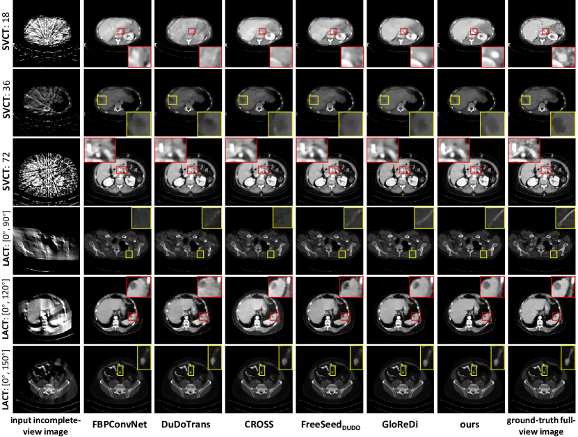
Figure 3: Visual comparison of state-of-the-art methods (from left to right) on DeepLesion dataset over different incomplete-view scenarios and settings (from top to bottom). The display windows [window width, window level] are set to [300, 35] HU for Row 1, 3 and 5; [1000, 350] HU for Row 4 and 6; [3000, 500] HU for Row 2. Regions of interest are zoomed in for better viewing.

4.2 Comparison with state-of-the-art models

We compare our ProCT with state-of-the-art single-setting models in the SVCT and LACT scenarios on the DeepLesion test set, as shown in Tab. 1. Notably, while one would have to train multiple versions of these models for different settings, ProCT only needs to be employed and trained once to cover them all.

Quantitative results.

Tab. 1 shows that, in a setting where relatively more views are given (e.g., ${N_{\mathrm{view}}}=144$ for SVCT; an angular range of $R=[0^{\circ},150^{\circ}]$ for LACT), dual-domain methods exhibit clear superiority over image-domain ones due to the rich information provided by the sinogram. However, this superiority would diminish with fewer views. We also find that LACT scenario is more challenging, where the sinogram completion poses a more challenging extrapolation problem rather than simpler interpolation as typically in SVCT. This is more evident for dual-domain methods: note that an angular range $R=[0^{\circ},90^{\circ}]$ in LACT indicates a 87.5% drop of sinogram-domain information, but dual-domain models like DuDoTrans and FreeSeed_dudo perform even worse than their corresponding SVCT versions in ${N_{\mathrm{view}}}=18$ that indicates a 97.5% drop. This is because the unsuccessful sinogram extrapolation in those dual-domain methods without particular designs may accumulate errors, leading to limited performance gains. In contrast, our ProCT outperforms the single-setting models in most of the settings, and achieves the best performance in terms of average metrics.

Additionally, we assess whether the ability of universal incomplete-view CT reconstruction can be simply unlocked by applying our multi-setting training strategy. For the most performing single-setting models GloReDi and FreeSeed_dudo, we develop two variants: (1) FreeSeed${}^{*}_{\textsc{dudo}}$, and (2) GloReDi^∗, both of which are trained following the same multi-setting training strategy as with our model. FreeSeed${}^{*}_{\textsc{dudo}}$ and GloReDi^∗ have the same architecture as their single-setting counterparts.

As shown in Rows 8 and 9 of Tab. 1, FreeSeed${}^{*}_{\textsc{dudo}}$ and GloReDi^∗ perform worse than their single-setting counterparts, indicating that the non-trivial transferability of ProCT stems from within our model rather than the training strategy. This observation is also in line with previous findings [11] that, without proper design, training with incomplete-view CT data under different CT settings can adversely impact the learning process and lead to poor performance. In contrast, with the view prompt and the artifact-aware contextual learning, our ProCT achieves better performance in most of the incomplete-view CT settings using only one single model.

Qualitative results.

Fig. 3 shows the reconstructed incomplete-view CT images by different methods, where the regions of interest are zoomed in to aid visualization. One can observe that, while dual-domain methods achieve higher quantitative results in certain settings, they can fail to recover the detail in the degraded CT images or produce distorted results, such as the aorta in Row 1, the bone structure in Row 4, and the splenic lesion in Row 5. More visualization examples can be found in our supplementary material.

4.3 Evaluation on unseen dataset and scenario

Generalizing on a new dataset.

We apply the above models trained using the DeepLesion dataset to the AAPM test set without any fine-tuning for further evaluation of the generalizability. The quantitative results are shown in Tab. 2. While dual-domain models like FreeSeed${}_{\textsc{dudo}}$ typically generalize worse on the challenging LACT scenario than on the SVCT scenario, the proposed ProCT achieves better average performance for both scenarios, showing strong generalizability of our model on a new dataset.

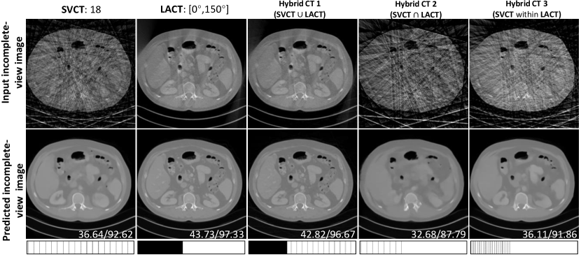
Figure 4: ProCT can easily adapt to out-of-domain hybrid CT scenarios. PSNR/SSIM values are displayed in the corner of the image; The last row shows the input view prompt.

Table 2: Quantitative evaluation [PSNR (db), SSIM (%)] for the generalizability of state-of-the-art methods on the AAPM dataset. The best results are highlighted in bold and the second best results are underlined.

	SVCT										LACT
	${N_{\mathrm{view}}}=18$		${N_{\mathrm{view}}}=36$		${N_{\mathrm{view}}}=72$		${N_{\mathrm{view}}}=144$		avg.		$R=[0^{\circ},90^{\circ}]$		$R=[0^{\circ},120^{\circ}]$		$R=[0^{\circ},150^{\circ}]$		avg.
Method	PSNR	SSIM	PSNR	SSIM	PSNR	SSIM	PSNR	SSIM	PSNR	SSIM	PSNR	SSIM	PSNR	SSIM	PSNR	SSIM	PSNR	SSIM
single-setting models
FBP	22.46	35.68	25.71	48.56	30.89	66.52	36.33	84.50	28.85	58.82	18.78	58.89	23.44	70.17	28.85	78.54	23.69	69.20
DDNet [32]	34.74	90.70	37.61	92.17	41.39	95.99	44.42	97.49	39.54	94.09	33.20	92.04	37.37	95.57	41.67	97.34	37.55	94.98
FBPConvNet [7]	35.00	89.70	38.06	92.58	41.75	95.54	45.18	97.95	40.00	93.94	33.60	92.60	38.95	96.19	43.14	97.52	38.56	95.43
DuDoTrans [24]	35.29	91.47	38.61	94.15	42.20	96.68	45.86	98.22	40.49	95.13	31.36	91.07	36.91	95.82	42.31	98.13	36.86	95.00
CROSS [6]	35.00	91.32	37.92	93.84	39.82	95.80	43.05	97.46	38.94	94.61	34.89	93.54	38.49	95.72	43.67	97.77	39.01	95.67
FreeSeeddudo [13]	35.35	91.51	38.61	94.35	42.23	96.73	45.77	98.19	40.48	95.20	32.65	92.85	38.37	96.74	43.68	98.27	38.23	95.95
GloReDi [11]	36.06	92.18	39.47	95.16	41.85	96.62	44.71	97.64	40.52	95.40	35.13	94.26	39.18	96.57	43.81	97.95	39.38	96.26
multi-setting models
UniverSeg [4]	33.09	89.53	36.83	92.81	41.01	95.85	44.21	97.58	38.78	94.94	31.61	91.60	36.15	95.35	40.13	97.18	35.96	94.71
ProCT (ours)	36.38	92.76	39.48	95.01	42.35	96.78	45.34	97.96	40.89	95.63	36.74	95.04	40.50	97.03	44.29	98.05	40.51	96.70

Adapting to out-of-domain scenarios.

Further, we find that ProCT can also generalize on or adapt to new hybrid CT scnarios. Here, we manipulate an LACT angular range of $[0^{\circ},150^{\circ}]$ and a SVCT number of views of $18$ to create three out-of-domain hybrid CT scenarios: “Hybrid CT 1” which is the union of LACT and SVCT, “Hybrid CT 2” which is the intersection, and “Hybrid CT 3” which does SVCT within the angular range of LACT, and evaluate the performance of ProCT on these scenarios.

The incomplete-view images in the “Hybrid CT 1” scenario have only subtle differences compared with ones in the $[0^{\circ},150^{\circ}]$-LACT scenario, so we directly apply our well-trained ProCT to them without re-training. However, the other two scenarios exhibiting pronounced artifacts are much more difficult to generalize. To solve this problem, we only fine-tune the prompter for 3 epochs on the DeepLesion dataset to create two versions specifically for “Hybrid CT 2” and “Hybrid CT 3”, while all other parameters of ProCT are frozen. A typical CT sample is shown in Fig. 4. Despite the complex artifacts in the input hybrid CT image, ProCT still manages to remove the artifact and restore the image content. Note that adapting ProCT to all these unseen scenarios requires minimal or no fine-tuning.

4.4 Ablation studies

We validate the effectiveness of our designs by comparing the default version of ProCT and other variants in Tab. 3. The configurations are as follows: (1) default version (“phantom pair w/ $\boldsymbol{p}$”); (2) removing view prompt from the default (“default w/o $\boldsymbol{p}$”); (3) replacing phantom pair in the default version with random real incomplete- and full-view CT image pairs in the DeepLesion training set (“real pair w/ $\boldsymbol{p}$”); (4) replacing phantom pair with the input incomplete-view CT image, i.e., no extra information is provided (“no context w/ $\boldsymbol{p}$”); (5) replacing phantom pair with an incomplete-view phantom image (“incomplete-view phantom w/ $\boldsymbol{p}$”); and (6) replacing phantom pair with a full-view phantom image (“full-view w/ $\boldsymbol{p}$”).

Ablation on the view prompt.

By comparing Rows 1 and 2 of Tab. 3, we observe that the variant without the view prompt is still aware of different incomplete-view CT settings, thanks to the artifact pattern information in the contextual pair. Unfortunately, this information is limited for effectively discriminating the fine-grained settings, leading to sub-optimal performance. In contrast, the proposed view prompt benefits our model by injecting the setting-discriminative information.

With proper modification, we can also set the view prompts to be learnable vectors during training, which is discussed in Sec. C1 of our supplementary material.

Table 3: Ablation on different configurations.

Configurations	SVCT-PSNR	SVCT-SSIM	LACT-PSNR	LACT-SSIM
(1) phantom pair w/ $\boldsymbol{p}$ (default)	39.73	93.82	41.33	94.93
(2) phantom pair w/o $\boldsymbol{p}$	37.69	91.68	37.79	92.47
(3) real pair w/ $\boldsymbol{p}$	39.80	93.90	41.32	95.07
(4) no context w/ $\boldsymbol{p}$	39.57	93.23	41.00	94.49
(5) incomplete-view phantom w/ $\boldsymbol{p}$	38.27	90.55	39.29	92.62
(6) full-view phantom w/ $\boldsymbol{p}$	38.07	91.20	39.44	93.34

Ablation on the contextual learning.

Rows 1 and 4 of Tab. 3 demonstrates the effectiveness of artifact-aware contextual learning. While CT phantom is chosen as our default context considering its easy access, the contextual pair can also be created from real incomplete- and full-view CT image pairs, when they are available.

Row 3 in Tab. 3 shows that choosing real CT image pair as context achieves better performance. We attribute this improvement to the increased artifact similarity between the contextual pairs and the source CT images, as the contextual image pair is derived from real CT images and may offer a more accurate guidance for the model to adeptly mitigate the signal-dependent artifacts in the input incomplete-view CT images. By comparing Rows 1 and 6 in Tab. 3, we also find that either the single incomplete-view phantom or the full-view one alone performs even worse than using no contextual information, which indicates that the effectiveness of our model may be attributed to the utilization of incomplete- and full-view pairs as context that aids the learning of mapping from degraded to clean images.

Despite the benefit of real CT image pairs, we opt for CT phantom as our contextual pair since it is more reliably accessible in clinical practice, offering a pragmatic solution when real patient data is unavailable.

5 Conclusion

In this paper, we present a universal and effective artifact removal model, termed ProCT, for the challenging task of universal incomplete-view CT reconstruction with diverse practical settings. By incorporating the view-aware prompting and the artifact-aware contextual learning, ProCT can resolve a wide range of incomplete-view CT reconstruction settings using a single image-domain model, greatly reducing the burden of computational resources for the related medical institutions. Extensive experiments also show that, ProCT does not require sinogram-domain data, yet achieves competitive or even better reconstruction performance compared to the dominating dual-domain methods, demonstrating the effectiveness and applicability of our proposed model. Limitations are discussed in Sec. E.

Supplementary Material

Appendix A Network Architecture

Our proposed model ProCT has an hourglass architecture with skip connection, with three encoding stages (including a bottleneck stage) and two decoding stages. Each stage contains several transformer blocks and the detailed configurations are shown in Tab. S1. To reduce the computational burden, we do not insert W-MHSA in every transformer block and use an “attention ratio” parameter to indicate the percentage of transformer blocks containing W-MHSA.

Within the network, two separate pathways are employed, namely the source pathway and the context pathway. The source pathway is for the input source incomplete-view CT image, while the context pathway deals with the incomplete- and full-view contextual pair. The patch embedding, patch unembedding, normalization, and MLP layers are independently applied for two pathways. Specifically, to adapt the vision transformer to our image-domain CT reconstruction task, we replace the vanilla layer normalization layer with rescaled layer normalization layer [21], which better preserves the brightness and contrast information that is crucial for low-level vision task.

Table S1: Detailed architecture configurations.

Configurations	Values
Embedding dimension	[24,48,96,48,24]
Number of transformer blocks	[8,8,8,4,4]
Number of heads for W-MHSA	[2,4,6,1,1]
Window size for W-MHSA	[8,8,8,8,8]
MLP ratio	[2,4,4,2,2]
Attention ratio	[0,1/2,1,0,0]

Appendix B Detailed Experimental Setup

B.1 Data preparation

The TorchRadon toolbox [18] is employed to simulate the fan-beam CT routine under 120 kVp and 500 mA. The distance between source and rotation center, as well as detectors and rotation center, is 1075 mm each. The number of detectors is set to 672.

To simulate the photon noise in the real-world CT scenarios, we add mixed noise comprising Poisson noise at an intensity of $10^{6}$ and zero-mean Gaussian noise with a 0.01 standard deviation to the sinograms that generate the CT images. Note that, different from the previous methods [11], the ground-truth full-view CT images for training are also generated from the noisy sinograms, which increase the difficulty of the optimization process but is more consistent with the practice of training with clinical data.

B.2 Storage requirement of models

We also provide a comparison of storage requirements in Tab. S2. Some values are marked with “$\times$7”, because 7 versions of the corresponding model should be stored in total to deal with all 7 settings in Tabs. 1 and 2. In contrast, only one model of ProCT needs to be stored.

Table S2: Storage requirement for different models.

Method	DDNet [32]	FBPConvNet [7]	DuDoTrans [24]	CROSS [6]	GloReDi [11]	FreeSeeddudo [13]	UniverSeg [4]	ours
Storage (M)	2.27$\times$7	131$\times$7	66.8$\times$7	139$\times$7	51.9$\times$7	184$\times$7	4.53	25.7

Appendix C More Ablation Studies

C.1 Ablation on the prompt

While we propose to adopt the sampling vector to form our view prompts, we find that the prompts can also be parameterized by a set of learnable vectors. However, due to the abundance of incomplete-view CT settings (e.g., SVCT can have a wide range of $N_{\mathrm{view}}$ choices), it is impractical to directly assign a separate learnable prompt for each setting.

To solve this problem, for each CT scenario (SVCT and LACT), we manually divide the settings into several groups according to the reconstruction difficulty, and then assign a learnable vector that ranges within $[0,1]$ for each group. For example, SVCT incomplete-view images with $9\leq N_{\mathrm{view}}<18$ are much harder to restore than those with $72\leq N_{\mathrm{view}}<144$.

Then, we train a variant of our model (dubbed “learnable prompt”) under the same conditions as our default version. The quantitative results, presented in Tab. S3, indicate that although this eliminates the need for the sampling vector, it requires manual presetting and results in reduced performance compared to our original method with a deterministic prompt derived from the sampling vector.

Also, despite showing certain patterns, the learned prompts still lack interpretability, as displayed in Fig. S1.

Table S3: Ablation study on the sinogram sparsity prompt.

variants	SVCT-PSNR	SVCT-SSIM	LACT-PSNR	LACT-SSIM
learnable prompt	39.43	92.35	40.56	92.86
default	39.73	93.82	41.33	94.93

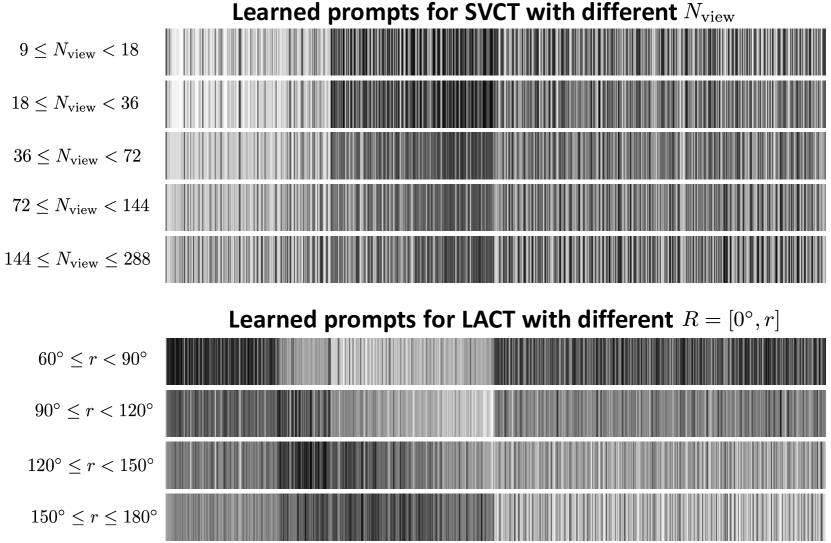
Figure S1: Visualization of learned view prompts for different incomplete-view CT settings.

C.2 Ablation on the loss function

We notice that the predicted incomplete-view CT images under difficult settings (e.g., ${N_{\mathrm{view}}}=18,36$ in SVCT) inherently lead to larger scales of loss. To mitigate the potential bias towards these settings, we handcraft a scaling schedule for the loss in Eq. (6), as shown in Fig. S2. The scaling factor $s_{t}$ grows as the setting becomes easier, and its effectiveness is evident by comparing Rows 3 and 5 of Tab. S4.

Table S4: Ablation study on the balancing factor $\alpha$ and the scaling schedule $s_{t}$.

	SVCT										LACT
	${N_{\mathrm{view}}}=18$		${N_{\mathrm{view}}}=36$		${N_{\mathrm{view}}}=72$		${N_{\mathrm{view}}}=144$		avg.		$R=[0^{\circ},90^{\circ}]$		$R=[0^{\circ},120^{\circ}]$		$R=[0^{\circ},150^{\circ}]$		avg.
Method	PSNR	SSIM	PSNR	SSIM	PSNR	SSIM	PSNR	SSIM	PSNR	SSIM	PSNR	SSIM	PSNR	SSIM	PSNR	SSIM	PSNR	SSIM
$\alpha=0$ w/ $s_{t}$	35.36	88.11	38.17	92.50	41.24	96.10	44.22	97.68	39.75	93.60	37.87	93.32	41.46	95.57	44.73	97.08	41.35	95.32
$\alpha=0.01$ w/ $s_{t}$	35.35	88.25	38.12	92.50	41.19	95.96	44.21	97.61	39.72	93.58	37.82	93.40	41.38	95.53	44.71	97.13	41.30	95.35
$\alpha=0.1$ w/ $s_{t}$	35.40	88.29	38.16	92.72	41.20	96.12	44.21	97.59	39.74	93.68	37.84	93.49	41.42	95.79	44.69	97.20	41.32	95.49
$\alpha=1$ w/ $s_{t}$	34.37	88.55	37.11	93.04	41.10	95.96	43.05	97.45	38.90	93.75	36.15	93.58	40.72	95.67	43.96	97.00	40.28	95.42
$\alpha=0.1$ w/o $s_{t}$	35.96	89.40	38.74	93.43	40.26	94.91	43.01	96.34	39.49	93.52	38.11	93.49	40.68	94.34	42.95	96.30	40.58	94.71

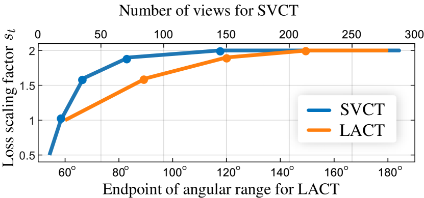
Figure S2: The proposed loss scaling schedule $s_{t}$ for different incomplete-view CT settings $t$.

In Eq. (6), we introduce a factor $\alpha$ for balancing the $\ell_{1}$ loss term $\mathcal{L}_{\ell_{1}}$ and the multi-scale structural similarity term $\mathcal{L}_{\mathrm{ssim}}$. We select $\alpha$ by comparing multiple versions of ProCT trained with loss scaling schedule using various $\alpha$ on the validation set, as shown in Tab. S4. While $\ell_{1}$ loss encourages pixel-wise alignment between the reconstructed result and the ground-truth full-view CT image and improves PSNR, multi-scale structural similarity loss $\mathcal{L}_{\mathrm{ssim}}$ mainly boosts the performance in terms of statistics. We find that $\alpha=0.1$ is a good choice for balancing these two types of loss. Based on $\alpha=0.1$, we also found that ProCT trained without the proposed loss scaling schedule, dubbed “$\alpha=0.1$ w/o $s_{t}$” in Tab. S4, presents a performance drop in the average metrics, showing the effectiveness of the schedule.

C.3 Ablation on the contextual learning

Qualitative evaluation of contextual pairs.

We first demonstrate the effectiveness of the contextual phantom pairs by providing some visualization examples of the default version of our model (“phantom pair”) and a variant that utilizes no contextual information (“no context”), as mentioned in Sec. 4.4. As shown in Fig. S4, our model can better restore the bone structure and the contour of the atrium and ventricle when using contextual pairs.

Ablation on the context selection.

Additionally, we explore two other variants as shown in Rows 2 and 3 of Tab. S5: (1) “phantom residue w/ $\boldsymbol{p}$”, where we use the residue of the full-view phantom image and the incomplete-view phantom image as context; (2) “no context w/o $\boldsymbol{p}$”, where no prompt nor contextual information is given to the network.

Although the phantom residue can also provide cues on the typical patterns of the incomplete-view CT artifact, it still leads to performance decline compared to our default version, as can be seen in Rows 1 and 2 of Tab. S5. This is because the pixel values in the residue present a larger dynamic range and steeper landscape, leading to misalignment with the input space and adding difficulty for the convergence. Additionally, the effectiveness of the proposed view prompt and the contextual pairs can be further demonstrated by comparing Rows 1 and 3 of Tab. S5.

Ablation on the real contextual pairs.

Despite being less consistently available, contextual pairs created from real incomplete- and full-view CT images benefit the artifact removal of our model, and introduce other intriguing questions that will be explored here. For example, the number of contextual images can affect the performance. Tab. S5 shows that the best reconstruction performance is achieved when three real CT contextual pairs are given, since fewer contextual pairs may result in a biased prediction while too many pairs cause interference.

Table S5: Ablation on more configurations.

Configurations	SVCT-PSNR	SVCT-SSIM	LACT-PSNR	LACT-SSIM
(1) phantom pair w/ $\boldsymbol{p}$ (default)	39.73	93.82	41.33	94.93
(2) phantom residue w/ $\boldsymbol{p}$	38.37	92.12	39.60	93.54
(3) no context w/o $\boldsymbol{p}$	34.16	84.02	32.94	84.51
(4) 1 real pair w/ $\boldsymbol{p}$	39.80	93.90	41.33	95.07
(5) 2 real pairs w/ $\boldsymbol{p}$	39.83	93.96	41.36	95.16
(6) 3 real pairs w/ $\boldsymbol{p}$	39.80	93.76	41.46	95.23
(7) 4 real pairs	39.20	93.39	40.92	94.92

Additionally, we investigate the impact of using real CT contextual pairs to determine what makes effective contexts for ProCT. First, from the AAPM test set, we select three typical incomplete-view CT images visualizing various positions of the body, respectively, as the input image. For each of them, we then test our ProCT on it, trying every contextual pairs from all other images in the AAPM dataset excluding those in the test set to search for the “best” one that leads to the highest PSNR in the inference.

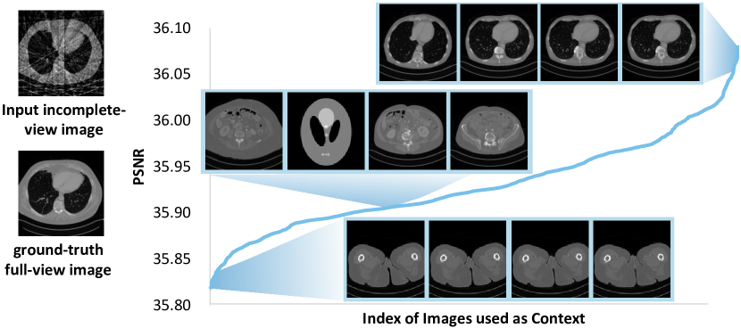
Figure S3: The more similar the content of the input image and the contextual image, the better the reconstruction of ProCT will be. Incomplete-view contextual images are omitted here for better visualization.

In Fig. S3, we visualize the contextual images corresponding to top-4 and bottom-4 PSNR values for ProCT’s restoration of the input SVCT chest image (${N_{\mathrm{view}}}=18$). We also indicate the location of CT phantom context and other images that lead to similar PSNR values as CT phantom. The result suggests that the contextual images that share similar content with the input image benefit ProCT for better restoration.

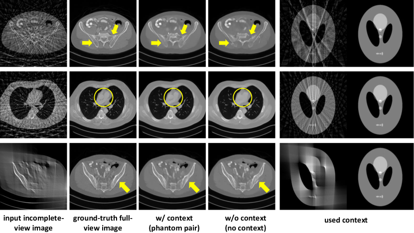
Figure S4: Contextual CT image pairs assist the restoration of some critical structures in the input incomplete-view CT image.

Appendix D More Visualization Examples

D.1 Different datasets

We provide more visualization examples of the reconstructed incomplete-view CT images from DeepLesion dataset for state-of-the-art methods in Fig. S5, and the examples from AAPM dataset are displayed in Fig. S6. Among these methods, our proposed ProCT produces images with better quality, as can be seen in Fig. S5, where the details of the kidney (Row 1), right upper lobe of the lung (Row 5), and other tissues (Row 6) are well maintained. In Fig. S6, some small structures missed in the images reconstructed by other methods can be restored by ProCT, as indicated by arrows in the figures.

Interestingly, dual-domain methods can capture the noise in the ground-truth images. This noise is induced by the mixed noise added to the source sinogram data, resulting in the granular texture in the CT image. On the other hand, image-domain methods generally learn to remove this noise, probably by working in a self-supervised manner [9], which indicates that image-domain methods can be potentially robust to the granular noise in the input CT image.

D.2 Different settings

Figs. S7 and S8 present the reconstructed results for two incomplete-view CT examples from the AAPM dataset with different incomplete-view CT settings. Note that $R\in\{[0^{\circ},50^{\circ}],[0^{\circ},250^{\circ}]\}$ in LACT and $N_{\text{view}}\in\{8,320\}$ in SVCT are out-of-domain settings. One can see that our universal model ProCT restores these images with satisfying visual quality in most settings, as well as the promising quantitative performance shown in the corresponding performance profiles.

However, ProCT can fail in some cases, especially in incomplete-view CT settings with extremely few views since most of the information is contaminated by severe artifacts. Also, in these cases, losing even one or two views can result in drastically different artifact patterns, which may be difficult for ProCT to remove.

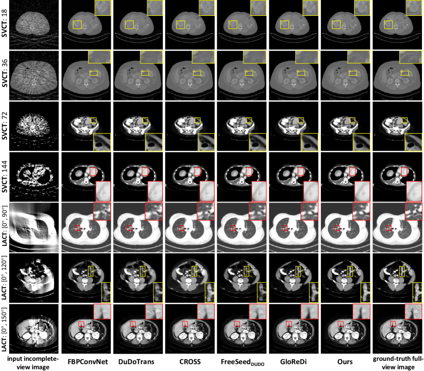
Figure S5: Visual comparison of state-of-the-art methods (from left to right) on DeepLesion dataset over different incomplete-view scenarios and settings (from top to bottom). The display windows [window width, window level] are set to [3000, 500] HU for Row 1 and 2; [300, 35] HU for Row 3, 4, 6, and 7; [1300, -600] HU for Row 5. Regions of interest are zoomed in for better viewing.

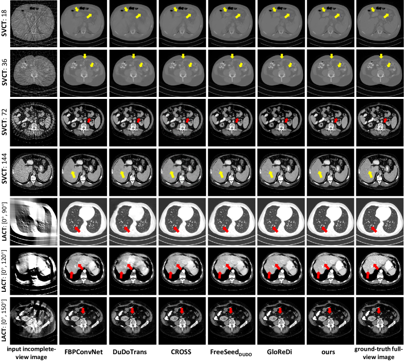
Figure S6: Visual comparison of state-of-the-art methods (from left to right) on AAPM dataset over different incomplete-view scenarios and settings (from top to bottom). The display windows [window width, window level] are set to [3000, 500] HU for Row 1 and 2; [300, 35] HU for Row 3, 4, 6, and 7; [1300, -600] HU for Row 5. Regions of interest are indicated by arrows in the figures.

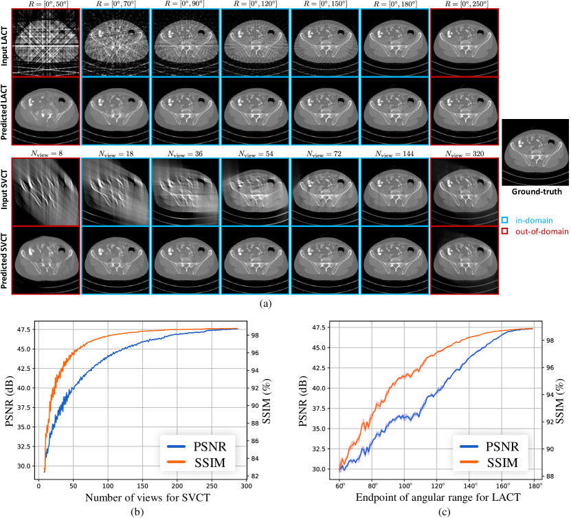
Figure S7: An example of images reconstructed by ProCT under different incomplete-view CT scenarios and settings. For each CT scenario and the corresponding exemplar image, 7 settings are visualized. (a) Reconstructed results; (b) SVCT performance profile; (c) LACT performance profile.

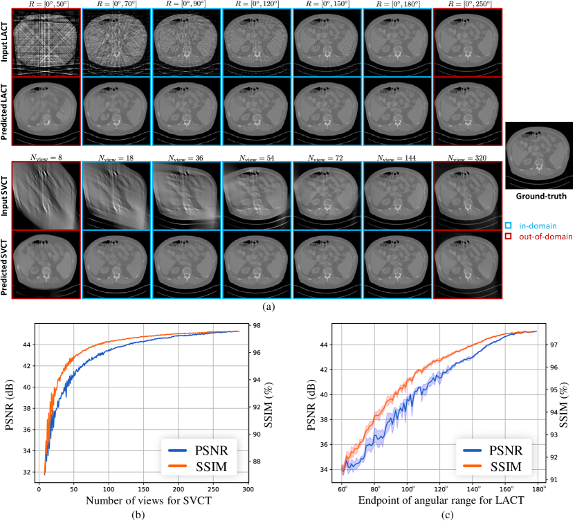
Figure S8: Another example of images reconstructed by ProCT under different incomplete-view CT scenarios and settings. For each CT scenario and the corresponding exemplar image, 7 settings are visualized. (a) Reconstructed results; (b) SVCT performance profile; (c) LACT performance profile.

Appendix E Limitation

Despite the inspiring all-in-one reconstruction performance and the low storage requirement of ProCT, some issues exist that our method did not fully address. For example, the lack of sinogram domain information leads to over-smoothed images in the predicted image-domain reconstruction, particularly in those settings with extremely few views. This problem may be further tackled by utilizing other strong and robust prior or using a specially designed loss function. Also, the inference speed of ProCT is lower than previous image-domain methods, because of the dual-pathway computation and the multiple layers of self-attention in ProCT. In the future, we plan to look into these issues and build a more efficient and generalizable universal model that produces high-quality CT images for incomplete-view CT reconstruction.

References

- Arai et al. [2001] Yoshinori Arai, Kazuya Honda, Kazuo Iwai, and Koji Shinoda. Practical model 3DX of limited cone-beam x-ray ct for dental use. In International Congress Series, pages 713–718, 2001.
- Bar et al. [2022] Amir Bar, Yossi Gandelsman, Trevor Darrell, Amir Globerson, and Alexei A Efros. Visual prompting via image inpainting. In Advances in Neural Information Processing Systems, 2022.
- Brown et al. [2020] Tom Brown, Benjamin Mann, Nick Ryder, Melanie Subbiah, Jared D Kaplan, Prafulla Dhariwal, Arvind Neelakantan, Pranav Shyam, Girish Sastry, Amanda Askell, Sandhini Agarwal, Ariel Herbert-Voss, Gretchen Krueger, Tom Henighan, Rewon Child, Aditya Ramesh, Daniel Ziegler, Jeffrey Wu, Clemens Winter, Chris Hesse, Mark Chen, Eric Sigler, Mateusz Litwin, Scott Gray, Benjamin Chess, Jack Clark, Christopher Berner, Sam McCandlish, Alec Radford, Ilya Sutskever, and Dario Amodei. Language models are few-shot learners. In Advances in Neural Information Processing Systems, pages 1877–1901, 2020.
- Butoi et al. [2023] Victor Ion Butoi, Jose Javier Gonzalez Ortiz, Tianyu Ma, Mert R Sabuncu, John Guttag, and Adrian V Dalca. UniverSeg: Universal medical image segmentation. arXiv preprint arXiv:2304.06131, 2023.
- Cho and Fessler [2013] Jang Hwan Cho and Jeffrey A Fessler. Motion-compensated image reconstruction for cardiac ct with sinogram-based motion estimation. In 2013 IEEE Nuclear Science Symposium and Medical Imaging Conference, pages 1–5, 2013.
- Hu et al. [2023] Dianlin Hu, Yikun Zhang, Guotao Quan, Jun Xiang, Gouenou Coatrieux, Shouhua Luo, Jean-Louis Coatrieux, Xu Ji, Hongbin Han, and Yang Chen. CROSS: Cross-domain residual-optimization-based structure strengthening reconstruction for limited-angle CT. IEEE Transactions on Radiation and Plasma Medical Sciences, 7(5):521–531, 2023.
- Jin et al. [2017] Kyong Hwan Jin, Michael T McCann, Emmanuel Froustey, and Michael Unser. Deep convolutional neural network for inverse problems in imaging. IEEE Transactions on Image Processing, 26(9):4509–4522, 2017.
- Kingma and Ba [2014] Diederik P. Kingma and Jimmy Ba. Adam: A method for stochastic optimization. arXiv preprint arXiv:1412.6980, 2014.
- Lehtinen et al. [2018] Jaakko Lehtinen, Jacob Munkberg, Jon Hasselgren, Samuli Laine, Tero Karras, Miika Aittala, and Timo Aila. Noise2Noise: Learning image restoration without clean data. In Proceedings of the 35th International Conference on Machine Learning, pages 2965–2974, 2018.
- Li et al. [2022] Runrui Li, Qing Li, Hexi Wang, Saize Li, Juanjuan Zhao, Qiang Yan, and Long Wang. DDPTransformer: Dual-domain with parallel transformer network for sparse view ct image reconstruction. IEEE Transactions on Computational Imaging, 8:1101–1116, 2022.
- Li et al. [2023] Zilong Li, Chenglong Ma, Jie Chen, Junping Zhang, and Hongming Shan. Learning to distill global representation for sparse-view CT. In Proceedings of the IEEE/CVF International Conference on Computer Vision, pages 21196–21207, 2023.
- Liu et al. [2021] Ze Liu, Yutong Lin, Yue Cao, Han Hu, Yixuan Wei, Zheng Zhang, Stephen Lin, and Baining Guo. Swin transformer: Hierarchical vision transformer using shifted windows. In Proceedings of the IEEE/CVF International Conference on Computer Vision, pages 10012–10022, 2021.
- Ma et al. [2023a] Chenglong Ma, Zilong Li, Yi Zhang, Junping Zhang, and Hongming Shan. Freeseed: Frequency-band-aware and self-guided network for sparse-view ct reconstruction. In Medical Image Computing and Computer Assisted Intervention – MICCAI 2023, 2023a.
- Ma et al. [2023b] Jiaqi Ma, Tianheng Cheng, Guoli Wang, Xinggang Wang, Qian Zhang, and Lefei Zhang. ProRes: Exploring degradation-aware visual prompt for universal image restoration. arXiv preprint arXiv:2306.13653, 2023b.
- McCollough et al. [2017] Cynthia H. McCollough, Adam C. Bartley, Rickey E. Carter, Baiyu Chen, Tammy A. Drees, Phillip Edwards, David R. Holmes III, Alice E. Huang, Farhana Khan, Shuai Leng, Kyle L. McMillan, Gregory J. Michalak, Kristina M. Nunez, Lifeng Yu, and Joel G. Fletcher. Low-dose CT for the detection and classification of metastatic liver lesions: Results of the 2016 low dose CT grand challenge. Medical Physics, 44(10):e339–e352, 2017.
- Paszke et al. [2019] Adam Paszke, Sam Gross, Francisco Massa, Adam Lerer, James Bradbury, Gregory Chanan, Trevor Killeen, Zeming Lin, Natalia Gimelshein, Luca Antiga, et al. PyTorch: An imperative style, high-performance deep learning library. Advances in Neural Information Processing Systems, 32, 2019.
- Potlapalli et al. [2023] Vaishnav Potlapalli, Syed Waqas Zamir, Salman Khan, and Fahad Shahbaz Khan. PromptIR: Prompting for all-in-one blind image restoration. Advances in Neural Information Processing Systems, 2023.
- Ronchetti [2020] Matteo Ronchetti. TorchRadon: Fast differentiable routines for computed tomography. arXiv preprint arXiv:2009.14788, 2020.
- Sheng et al. [2020] Wenjuan Sheng, Xing Zhao, and Mengfei Li. A sequential regularization based image reconstruction method for limited-angle spectral ct. Physics in Medicine & Biology, 65(23):235038, 2020.
- Shu and Entezari [2022] Ziyu Shu and Alireza Entezari. Sparse-view and limited-angle CT reconstruction with untrained networks and deep image prior. Computer Methods and Programs in Biomedicine, 226:107167, 2022.
- Song et al. [2023] Yuda Song, Zhuqing He, Hui Qian, and Xin Du. Vision transformers for single image dehazing. IEEE Transactions on Image Processing, 32:1927–1941, 2023.
- Ulyanov et al. [2018] Dmitry Ulyanov, Andrea Vedaldi, and Victor Lempitsky. Deep image prior. In Proceedings of the IEEE Conference on Computer Vision and Pattern Recognition, pages 9446–9454, 2018.
- Valanarasu et al. [2022] Jeya Maria Jose Valanarasu, Rajeev Yasarla, and Vishal M Patel. Transweather: Transformer-based restoration of images degraded by adverse weather conditions. In Proceedings of the IEEE/CVF Conference on Computer Vision and Pattern Recognition, pages 2353–2363, 2022.
- Wang et al. [2022] Ce Wang, Kun Shang, Haimiao Zhang, Qian Li, and S. Kevin Zhou. DuDoTrans: Dual-domain transformer for sparse-view CT reconstruction. In Machine Learning for Medical Image Reconstruction, pages 84–94, 2022.
- Wang and Yu [2013] Ge Wang and Hengyong Yu. The meaning of interior tomography. Physics in Medicine & biology, 58(16):R161, 2013.
- Wang et al. [2008] Ge Wang, Hengyong Yu, and Bruno De Man. An outlook on X-ray CT research and development. Medical Physics, 35(3):1051–1064, 2008.
- Wang et al. [2023] Xinlong Wang, Wen Wang, Yue Cao, Chunhua Shen, and Tiejun Huang. Images speak in images: A generalist painter for in-context visual learning. In Proceedings of the IEEE/CVF Conference on Computer Vision and Pattern Recognition, pages 6830–6839, 2023.
- Wang et al. [2004] Zhou Wang, A.C. Bovik, H.R. Sheikh, and E.P. Simoncelli. Image quality assessment: from error visibility to structural similarity. IEEE Transactions on Image Processing, 13(4):600–612, 2004.
- Yan et al. [2018] Ke Yan, Xiaosong Wang, Le Lu, and Ronald M Summers. DeepLesion: Automated mining of large-scale lesion annotations and universal lesion detection with deep learning. Journal of Medical Imaging, 5(3):036501–036501, 2018.
- Zhang et al. [2022a] Yi Zhang, Hu Chen, Wenjun Xia, Yang Chen, Baodong Liu, Yan Liu, Huaiqiang Sun, and Jiliu Zhou. LEARN++: Recurrent dual-domain reconstruction network for compressed sensing CT. IEEE Transactions on Radiation and Plasma Medical Sciences, 7(2):132–142, 2022a.
- Zhang et al. [2022b] Yikun Zhang, Dianlin Hu, Shilei Hao, Jin Liu, Guotao Quan, Yi Zhang, Xu Ji, and Yang Chen. DREAM-Net: Deep residual error iterative minimization network for sparse-view CT reconstruction. IEEE Journal of Biomedical and Health Informatics, 27(1):480–491, 2022b.
- Zhang et al. [2018] Zhicheng Zhang, Xiaokun Liang, Xu Dong, Yaoqin Xie, and Guohua Cao. A sparse-view CT reconstruction method based on combination of DenseNet and deconvolution. IEEE Transactions on Medical Imaging, 37(6):1407–1417, 2018.
- Zhao et al. [2016] Hang Zhao, Orazio Gallo, Iuri Frosio, and Jan Kautz. Loss functions for image restoration with neural networks. IEEE Transactions on Computational Imaging, 3(1):47–57, 2016.