On the construction of stationary processes and random fields

Abstract.

We propose a new method to construct a stationary process and random field with a given convex, decreasing covariance function and any one-dimensional marginal distribution. The result is a new class of stationary processes and random fields. The construction method provides a simple, unified approach for a wide range of covariance functions and any one-dimensional marginal distributions, and it allows a new way to model dependence structures in a stationary process/random field as its dependence structure is induced by the correlation structure of a few disjoint sets in the support set of the marginal distribution.

1. Introduction

In time series, a stationary process is modeled by the moving average of independent innovations or the autoregression of past observations. These methods work well for a wide range of dependence structures, from an exponentially decaying covariance function to a power-law decaying covariance function, when the marginal distribution is normal marginal distribution. It is desirable to develop models for stationary processes where the one-dimensional marginal distribution can be chosen to fit the type of data at hand, while the correlation structure is flexible [2]. In the past several decades, there has been much progress in constructing stationary processes with various marginal distributions.

In [9], a markovian process with exponential marginal distribution was developed. In [8], first-order stationary autoregressive models are introduced with non-Gaussian marginal distribution by using a latent variable for the transition density. The method was extended for a continuous-time Markov model in [7], and for broader marginal distributions in [3]. In [2], the sum of independent autoregressions was considered to construct a stationary process with a given marginal distribution and autocorrelation that has two or more time scales. A comprehensive account of other autoregressive models with non-Gaussian marginal can be found in [1].

Even though these models can account for a wide range of stationary processes, the marginal distributions are still restricted to self-decomposable distributions and the autocorrelations of the stationary processes are exponentially decaying since they are autoregressive/Markovian models with finite orders.

In this paper, we propose a new method to construct a stationary process with any given one-dimensional marginal distribution and a given covariance function that is convex and decreasing. Our method utilizes a sequence of binary random variables whose covariance function is proportional to the given covariance function. The dependence structure of the stationary process will be induced by the binary process whose states are linked to disjoint sets of the support set of the marginal distribution. This provides a different approach to model dependence in a stochastic process than existing moving average or autoregressive models as the dependence structure of the process is derived through a dependence structure among the disjoint sets in the marginal distribution of the process. When some set of values of a variable is known to be correlated and induces correlations in the time series, our method can be a useful tool to model such data. We also extend our method to construct a random field with a given marginal distribution and flexible covariance function.

In Section 2, we introduce a generalized Bernoulli process which is a stationary binary sequence that can have a wide range of covariance functions. In Section 3, we develop a method to construct a stationary process with a given one-dimensional marginal distribution and covariance function. We extend this method in Section 4 to propose a construction method for a random field with any one-dimensional marginal distribution and given covariance function. In Section 5, simulations of some of our stationary processes/random fields are presented, followed by concluding remarks in Section 6. All the proofs can be found in Section 7.

Throughout the paper, we will use bold font for a vector in two or more dimensions, and calligraphic font for a matrix. We assume $i,i_{0},i_{1},\cdots\in\mathbb{Z},$ and $\mathbf{s},\mathbf{t},\mathbf{t}_{1},\mathbf{t}_{2},\cdots\in\mathbb{Z}^{d},$ unless stated otherwise. For a random vector, its $i$th element is denoted with the subscript, e.g., $\mathbf{X}(i)=(X_{1}(i),X_{2}(i),\cdots,X_{d}(i))^{\prime}.$ For identically distributed random variables, we suppress the index of a random variable for its expected value, i.e., if $\mathbf{X}(i)=(X_{1}(i),X_{2}(i),\cdots,X_{d}(i)),i=1,2,\cdots,$ are i.i.d. random vectors, then we use $E(\mathbf{X}),$ $E(X_{k}),$ $E(e^{{\rm i}\mathbf{t}^{\prime}\mathbf{X}})$ for $E(\mathbf{X}(i)),E(X_{k}(i))$ and $E(e^{{\rm i}\mathbf{t}^{\prime}\mathbf{X}(i)}),$ respectively. For multiple integral with $\mathbf{x}=(x_{1},x_{2},\cdots,x_{d})$, we use notation $\int f(\mathbf{x})d\mathbf{x}$ for $\int\cdots\int f(x_{1},\cdots,x_{d})dx_{1}\cdots dx_{d}.$ For the union of disjoint sets, we use $\sqcup$, for indicator function, we use $I_{\{\cdot\}}$ or $I(\cdot),$ and $[n]$ denotes the set $\{1,2,\cdots,n\}.$

2. A Generalized Bernoulli Process

In [5], a generalized Bernoulli process (GBP) $\{\xi_{i},i\in\mathbb{N}\}$ was introduced as a stationary binary sequence that can possess long-range dependence (LRD). The covariance function of GBP was a power function

$$cov(\xi_{i},\xi_{i+k})=c|k|^{2H-2},$$

for some constants $c>0$ and $H\in(0,1),$ and when $H\in(0.5,1),$ GBP has LRD. Here, we extend GBP to a more general stationary binary sequence with a wide range of covariance functions that are decreasing and convex functions. Let $\xi_{i},i\in\mathbb{Z},$ be a binary sequence and $C(\cdot)$ be a decreasing, convex function defined on positive real line. We extend a GBP with the following probabilities.

$$P(\xi_{i}=1)=p,P(\xi_{i}=0)=1-p,$$

$$P(\xi_{i_{0}}=1,\xi_{i_{1}}=1,\cdots,\xi_{i_{n}}=1)=p\prod_{j=1}^{n}(p+C^{*}(i_{j}-i_{j-1})),$$

for $i_{0}<i_{1}<\cdots<i_{n},$ and $C^{*}(\cdot)=C(\cdot)/p.$ For any disjoint sets $B,F\subset\mathbb{Z},$

$$P(\cap_{i^{\prime}\in F}\{\xi_{i^{\prime}}=0\}\cap_{i\in B}\{\xi_{i}=1\})=\sum_{k=0}^{|F|}\sum_{\begin{subarray}{c}F^{\prime}\subset F\\ |F^{\prime}|=k\end{subarray}}(-1)^{k}P(\cap_{i\in F^{\prime}\cup B}\{\xi_{i}=1\}),\text{ and }$$

$$P(\cap_{i^{\prime}\in F}\{\xi_{i^{\prime}}=0\})=1+\sum_{k=1}^{|F|}\sum_{\begin{subarray}{c}F^{\prime}\subset F\\ |F^{\prime}|=k\end{subarray}}(-1)^{k}P(\cap_{i\in F^{\prime}}\{\xi_{i}=1\}).$$

To express the above probabilities more conveniently, define the following operators similarly as in [5].

Definition 2.1.

Define the following operation on a set $B=\{i_{0},i_{1},\cdots,i_{n}\}\subset\mathbb{Z}$ with $i_{0}<i_{1}<\cdots<i_{n}.$

$$L(B)=\prod_{j=1,\cdots,n}\Big{(}p+C^{*}(i_{j}-i_{j-1})\Big{)}.$$

If $B=\emptyset$, define $L(B):=1/p$, and if $|B|=1,L(B):=1.$

Definition 2.2.

Define for disjoint sets, $B,F\subset\mathbb{Z}$ with $|F|=m>0,$

$$D(B,F)=\sum_{j=0}^{|F|}\sum_{\begin{subarray}{c}F^{\prime}\subset F\\ |F^{\prime}|=j\end{subarray}}(-1)^{j}L(B\cup F^{\prime}).$$

If $F=\emptyset,D(B,F):=L(B).$

If $D(B,F)\geq 0$ for any disjoint sets $B,F\subset\mathbb{Z}$, GBP is well defined with probabilities

$$P(\cap_{i\in B}\{\xi_{i}=1\}\cap_{i^{\prime}\in F}\{\xi_{i^{\prime}}=0\}) =pD(B,F).$$ (2.1)

Especially,

$$P(\xi_{i}=\ell_{1},\xi_{j}=\ell_{2})=\prod_{k=1,2}p^{\ell_{k}}(1-p)^{\ell_{k}}+(-1)^{\ell_{1}+\ell_{2}}C(|i-j|)$$

for any $\ell_{1},\ell_{2}=0,1,$ therefore, it is a stationary process with covariance function $C,$

$$Cov(\xi_{i},\xi_{j})=C(|i-j|),i\neq j.$$

Here, we need the following assumption on a covariance function.

Assumption 2.3.

$C:[1,\infty)\to\mathbb{R}_{+}$ is a decreasing, convex function such that $C(1)<p(1-p)$ and $C(2)>(p^{2}+C(1))^{2}/p-p^{2}.$

In [5], it was shown that when the covariance function is a power function, $C(x)=c|x|^{2H-2}$, the parameters that satisfy Assumption 2.3 are $p,H\in(0,1),$ and

$$0\leq c<\min\{p(1-p),\frac{p}{2}(-2p+2^{2H-2}+\sqrt{4p-p2^{2H}+2^{4H-4}})\}.$$

Example 2.4.

A convex function, $C(x)=e^{-\theta x},\theta>0,$ satisfies Assumption 2.3 if $p\in(0,1),{\theta}\in(-\ln((-p^{2}+p\sqrt{p-p^{2}+p^{3}})/(1-p)),\infty).$ For $C(x)=ce^{-\theta x},$ if $\theta>0,c\in(0,p(1-p)),$ Assumption 2.3 is satisfied.

Example 2.5.

A convex function, $C(x)=ce^{-\theta x^{\alpha}},\theta>0,\alpha>0$ satisfies Assumption 2.3 if the following two conditions are met.

$$(a) \{\theta>0,\alpha>1\}\text{ or }\{\theta<1,\alpha\in(1,1/(1-\theta))\},$$

$$(b) c\in(0,e^{\theta}(p^{3/2}-p^{2})).$$

The next Theorem shows that under Assumption 2.3, GBP is well defined, i.e., $D(B,F)\geq 0$ for any disjoint sets $B,F\subset\mathbb{Z}.$

Theorem 2.6.

Under Assumption 2.3, GBP $\{\xi_{i},i\in\mathbb{Z}\}$ is well-defined stationary binary sequence with $P(\xi_{i}=1)=p,P(\xi_{i}=0)=1-p,$ and covariance function $C$.

We denote a GBP with a parameter $p$ and covariance function $C$ by $\xi_{i}\sim GBP(p,C).$

3. Construction of a Stationary Process

We will construct a discrete-time stationary process with any one-dimensional marginal distribution and a decreasing convex covariance function $C$ that satisfies Assumption 2.3. More specifically, We define a multivariate stationary process $\{\mathbf{X}(i)\in\mathbb{R}^{d},i\in\mathbb{Z}\}$, $d\in\mathbb{N},$ where $\mathbf{X}(i)$ follows any given one-dimensional marginal distribution. In fact, our method is easily extended with any probability space $(\Omega,F,P)$ for a marginal distribution, but for the sake of simplicity, we will assume that the marginal probability distribution has pdf $f(\mathbf{x}),\mathbf{x}\in\mathbb{R}^{d}.$ For the construction, we will utilize the GBP defined in Section 2.

Let $\xi_{i}\sim GBP(p,C)$ and $\mathbf{X}(i)=\mathbf{X}^{A}(i)I_{\{\xi_{i}=1\}}+\mathbf{X}^{A^{c}}(i)I_{\{\xi_{i}=0\}}$ where $\mathbf{X}^{A}(i)\in\mathbb{R}^{d},i\in\mathbb{Z},$ are i.i.d. random variables whose support set is $A\subset\mathbb{R}^{d}$ such that $\int_{A}f({\bf x})d{\bf x}=p$ and the pdf of $\mathbf{X}^{A}(i)$ is $f^{A}({\bf x})=f({\bf x})/p,{\bf x}\in A$. In the same way, $\mathbf{X}^{A^{c}}(i),i\in\mathbb{Z},$ are i.i.d. random variables whose support set is $A^{c}$ and its pdf is $f^{A^{c}}({\bf x})=f({\bf x})/(1-p),{\bf x}\in A^{c}$. Here, $f(\mathbf{x})$ can be any probability density function on $\mathbf{x}=(x_{1},x_{2},\cdots,x_{d})\in\mathbb{R}^{d}$. Also, $\{\mathbf{X}^{A}(i),i\in\mathbb{Z}\}$ and $\{\mathbf{X}^{A^{c}}(i),i\in\mathbb{Z}\}$ are independent of each other and also independent of $\{\xi_{i},i\in\mathbb{Z}\}$.

Theorem 3.1.

$\mathbf{X}(i)\in\mathbb{R}^{d},i\in\mathbb{Z},$ is a stationary process whose marginal probability density function is $f(\cdot)$ and variance-covariance matrix is

$$cov(\mathbf{X}(i),\mathbf{X}(j))=\mathscr{D}C(|i-j|),$$

where

$$\mathscr{D}_{k,\ell} =\Big{(}E(X_{k}^{A})-E(X_{k}^{A^{c}})\Big{)}\Big{(}E(X_{\ell}^{A})-E(X_{\ell}^{A^{c}})\Big{)}$$

$$=\frac{\int_{A}(x_{k}-\mu_{k})f({\bf x})d{\bf x}\int_{A}(x_{\ell}-\mu_{\ell})f({\bf x})d{\bf x}}{p^{2}(1-p)^{2}}$$

for $k,\ell=1,2,\cdots,d,$ and ${\bf\mu}=(\mu_{1},\mu_{2},\cdots,\mu_{d})^{\prime}=E(\mathbf{X}),$ i.e., $\mu_{k}=\int\cdots\int_{\mathbb{R}^{d}}x_{k}f({\bf x})d{\bf x}.$

For $q\in\mathbb{N},$ let $\mathbf{X}^{q}(i)=((X_{1}(i))^{q},\cdots,(X_{d}(i))^{q})^{\prime}$, $(\mathbf{X}^{A})^{q}(i)=((X_{1}^{A}(i))^{q},\cdots,(X_{d}^{A}(i))^{q})^{\prime},$ and $(\mathbf{X}^{A^{c}})^{q}(i)=((X_{1}^{A^{c}}(i))^{q},\cdots,(X_{d}^{A^{c}}(i))^{q})^{\prime},$ then we have the following result which can be proved in a similar way to Theorem 3.1.

Proposition 3.2.

In general, for $q\in\mathbb{N}$

$$cov(\mathbf{X}^{q}(i),\mathbf{X}^{q}(j))=\mathscr{D}^{(q)}C(|i-j|),$$

where $\mathscr{D}^{(q)}={\bf d}^{(q)}{\bf d}^{(q)^{\prime}},{\bf d}^{(q)}=E((\mathbf{X}^{A})^{q})-E((\mathbf{X}^{A^{c}})^{q}),$ i.e.,

$$\mathscr{D}^{(k)}_{k,\ell} =\Bigg{(}\frac{\int_{A}x_{k}^{q}f({\bf x})d{\bf x}}{p}-\frac{\int_{A^{c}}x_{k}^{q}f({\bf x})d{\bf x}}{1-p}\Bigg{)}\Bigg{(}\frac{\int_{A}x_{\ell}^{q}f({\bf x})d{\bf x}}{p}-\frac{\int_{A^{c}}x_{\ell}^{q}f({\bf x})d{\bf x}}{1-p}\Bigg{)}$$

$$=\frac{\int_{A}(x_{k}^{q}-\mu_{k}^{(q)})f({\bf x})d{\bf x}\int_{A}(x_{\ell}^{q}-\mu_{\ell}^{(q)})f({\bf x})d{\bf x}}{p^{2}(1-p)^{2}},$$

and $\mu_{k}^{(q)}=\int x_{k}^{q}f({\bf x})d{\bf x}$ for $k,\ell=1,2,\cdots,d.$

Proposition 3.3.

For any set $B_{1},B_{2}\subset\mathbb{R}^{d},$

$$cov(I_{\{\mathbf{X}(i)\in B_{1}\}},I_{\{\mathbf{X}(j)\in B_{2}\}})=d^{*}C(|i-j|),$$

where

$$d^{*}=\prod_{k=1,2}\Bigg{(}\frac{\int_{A\cap B_{k}}f({\bf x})d{\bf x}}{p}-\frac{\int_{A^{c}\cap B_{k}}f({\bf x})d{\bf x}}{1-p}\Bigg{)}.$$

Remark 3.4.

Proposition 3.3 indicates that the covariance between $I_{\{\mathbf{X}(i)\in B_{1}\}}$ and $I_{\{\mathbf{X}(j)\in B_{2}\}}$, for any $i,j\in\mathbb{Z},$ is maximized with $cov(I_{\{\mathbf{X}(i)\in B_{1}\}},I_{\{\mathbf{X}(j)\in B_{2}\}})=C(|i-j|)$ when $B_{1}=B_{2}=A\text{ or }B_{1}=B_{2}=A^{c}.$ On the other hand, the covariance is minimized with $cov(I_{\{\mathbf{X}(i)\in B_{1}\}},I_{\{\mathbf{X}(j)\in B_{2}\}})=-C(|i-j|)$ when $B_{1}=A,B_{2}=A^{c},$ or $B_{2}=A,B_{1}=A^{c}.$

Note that the joint pdf of $\{\mathbf{X}(i_{j}),j=1,2,\cdots,k\}$, for some $k\in\mathbb{N},\{i_{1},\cdots,i_{k}\}\subset\mathbb{Z},$ is

$$f(\mathbf{X}({i_{1}}),\cdots,\mathbf{X}({i_{k}}))=\sum_{B\sqcup F=[k]}\prod_{\ell\in B}I(\mathbf{X}({i_{\ell}})\in A)\prod_{\ell^{\prime}\in F}I(\mathbf{X}({i_{\ell^{\prime}}})\in A^{c})pD(B,F)\frac{\prod_{j=1}^{k}f(\mathbf{X}({i_{j}}))}{p^{|B|}(1-p)^{|F|}}.$$

Especially, for $k=2,$

$$f(\mathbf{X}(i),\mathbf{X}(j))=\sum_{\ell_{1},\ell_{2}=0,1}I(\mathbf{X}(i)\in A^{\ell_{1}},\mathbf{X}(j)\in A^{\ell_{2}})\bigg{(}1+\frac{(-1)^{\ell_{1}+\ell_{2}}C(|i-j|)}{\prod_{k=1,2}p^{\ell_{k}}(1-p)^{1-\ell_{k}}}\bigg{)}f(\mathbf{X}(i))f(\mathbf{X}(j))$$

where $A^{1}=A,A^{0}=A^{c}.$ The next proposition on the characteristic function of $\{\mathbf{X}(i),\mathbf{X}(j)\}$ is easily followed.

Proposition 3.5.

For $\theta_{j}\in\mathbb{R}^{d},j=1,2,$

$$E(e^{{\rm i}(\theta_{1}^{\prime}\mathbf{X}(i)+\theta_{2}^{\prime}\mathbf{X}(j))})=E(e^{{\rm i}\theta_{1}^{\prime}\mathbf{X}})E(e^{{\rm i}\theta_{2}^{\prime}\mathbf{X}})+C(|i-j|)\prod_{k=1,2}\Big{(}E\big{(}e^{{\rm i}\theta_{k}^{\prime}\mathbf{X}^{A}}\big{)}-E\big{(}e^{{\rm i}\theta_{k}^{\prime}\mathbf{X}^{A^{c}}}\big{)}\Big{)}.$$

Now we are ready to show the characteristic function of $\{\mathbf{X}(i_{j}),j=1,2,\cdots,k\}$ for any $i_{1},\cdots,i_{k}\in\mathbb{Z},k\in\mathbb{N}.$ Let $K\subset[k]=\{1,2,\cdots,k\},K\neq\emptyset.$ Define $K^{\circ}=\{j:j\in[k]/K,\min K<j<\max K\}$, and $Q_{K}$ as the set of partitions of $K$ such that for any $W\in Q_{K}$, it satisfies that $W=\{K_{i},i=1,2,\cdots,|W|\},$ where $K_{i}$ are disjoint, $|K_{i}|\geq 2,\sqcup_{i}K_{i}=K,$ and $\max{K_{i}}<\min{K_{j}}$ for $i<j.$ Note that $K\in Q_{K}.$ Also, define $W^{\circ}=\sqcup K_{i}^{\circ}$ for $W=\{K_{i},i=1,2,\cdots,|W|\}.$ Let $L^{*}(\{i_{1},i_{2},\cdots,i_{k}\})=p\prod_{j=2,3\cdots,k}C^{*}(i_{j}-i_{j-1})$ for any $i_{1}<i_{2}<\cdots<i_{k},k\in\mathbb{N}/\{1\},$ and for $W=\{K_{i},i=1,2,\cdots|W|\}\in Q_{K},$ $L^{*}(W)$ is defined as $\prod_{i=1}^{|W|}L^{*}(\{i_{j}:j\in K_{i}\})$.

Theorem 3.6.

For $\theta_{j}\in\mathbb{R}^{d},i_{j}\in\mathbb{Z},j=1,2,\cdots,k,k\in\mathbb{N}/\{1\},$

$$E(e^{{\rm i}\sum_{j=1,2,\cdots,k}\theta_{j}^{\prime}\mathbf{X}(i_{j})})=\prod_{j=1}^{k}E(e^{{\rm i}\theta_{j}^{\prime}\mathbf{X}})+$$

$$\sum_{\begin{subarray}{c}K\subset[k]\\ |K|\geq 2\\ W\in Q_{K}\end{subarray}}L^{*}(W)\prod_{j\in W^{\circ}}E(e^{{\rm i}\mathbf{t}_{j}^{\prime}\mathbf{X}^{A^{c}}})\prod_{i\in K}(E(e^{{\rm i}\theta_{i}^{\prime}\mathbf{X}^{A}})-E(e^{{\rm i}\theta_{i}^{\prime}\mathbf{X}^{A^{c}}}))\prod_{\ell\in[k]/(W^{\circ}\cup K)}E(e^{{\rm i}\theta_{\ell}^{\prime}\mathbf{X}}).$$

Theorem 3.6 implies that the multivariate stationary process $\{\mathbf{X}(i),i\in\mathbb{Z}\}$ becomes the sequence of i.i.d. random vectors if and only if $C\equiv 0,$ since the characteristic function of $\mathbf{X}^{A}$ cannot be the same as that of $\mathbf{X}^{A^{c}}$, as they have different support set, i.e., $E(e^{{\rm i}\mathbf{t}_{\ell}^{\prime}\mathbf{X}^{A}})\neq E(e^{{\rm i}\mathbf{t}_{\ell}^{\prime}\mathbf{X}^{A^{c}}}).$

4. Construction of a Stationary Random Field

In this section, we define a stationary multivariate random field $\mathbf{X}({\bf t})=(X_{1}(\mathbf{t}),X_{2}(\mathbf{t}),\cdots,X_{d}(\mathbf{t}))^{\prime}\in\mathbb{R}^{d}$ for ${\bf t}=(t_{1},t_{2})^{\prime}\in\mathbb{Z}^{2}$ with any one-dimensional marginal distribution and a convex, decreasing covariance function that satisfies Assumption 2.3. Let $\xi_{i}^{1},\xi_{i}^{2},i\in\mathbb{Z},$ be two independent GBPs, $\xi^{k}\sim GBP(p_{k},C_{k}),k=1,2.$

Let $f(\mathbf{x}),\mathbf{x}=(x_{1},\cdots,x_{d})\in\mathbb{R}^{d},$ be a pdf of any one-dimensional marginal distribution, and define for ${\bf t}=(t_{1},t_{2})^{\prime}\in\mathbb{Z}^{2},$

$$\mathbf{X}({\bf t})=\sum_{\ell_{1},\ell_{2}=0,1}\mathbf{X}^{A^{\ell_{1}\ell_{2}}}({\bf t})I({\xi_{t_{1}}^{1}=\ell_{1},\xi_{t_{2}}^{2}=\ell_{2}})$$

where $A^{11},A^{10},A^{01},A^{00}\subset\mathbb{R}^{d}$ are disjoint sets such that $\int_{A^{\ell_{1}\ell_{2}}}f({\bf x})d{\bf x}=\prod_{k=1,2}(p_{k})^{\ell_{k}}(1-p_{k})^{(1-\ell_{k})}$ and $\mathbf{X}^{A^{\ell_{1}\ell_{2}}}({\bf t})\in\mathbb{R}^{d},{\bf t}\in\mathbb{Z}^{2},$ are i.i.d. with pdf

$$f^{A^{\ell_{1}\ell_{2}}}(\mathbf{x})=\frac{f(\mathbf{x})I(\mathbf{x}\in A^{\ell_{1}\ell_{2}})}{\prod_{k=1,2}p_{k}^{\ell_{k}}(1-p_{k})^{1-\ell_{k}}}$$

for $\ell_{1},\ell_{2}=0,1.$ Also, the four sequences $\{\mathbf{X}^{A^{\ell_{1}\ell_{2}}}({\bf t}),{\bf t}\in\mathbb{Z}^{2}\},\ell_{1},\ell_{2}=0,1,$ are independent of each other, and also independent of $\{\xi_{i}^{1},\xi_{i}^{2},i\in\mathbb{Z}\}.$

Theorem 4.1.

$\{\mathbf{X}(\mathbf{t})\in\mathbb{R}^{d},{\bf t}\in\mathbb{Z}^{2}\}$ is a stationary random field whose marginal probability density function is $f(\cdot)$ and covariance function

$$C_{X}({\bf t}-{\bf s})=cov(\mathbf{X}(\mathbf{t}),\mathbf{X}(\mathbf{s}))=\mathscr{M}_{0}C_{1}(|t_{1}-s_{1}|)C_{2}(|t_{2}-s_{2}|)+\sum_{j=1,2}\mathscr{M}_{j}C_{j}(|t_{j}-s_{j}|),$$

where $\mathscr{M}_{i}=\mathbf{m}_{i}\mathbf{m}_{i}^{\prime}$ for $i=0,1,2,$ with

$$\mathbf{m}_{0} =E(\mathbf{X}^{A^{10}})+E(\mathbf{X}^{A^{01}})-E(\mathbf{X}^{A^{11}})-E(\mathbf{X}^{A^{00}}),$$ (4.1)

$$\mathbf{m}_{1} =p_{2}\Big{(}E(\mathbf{X}^{A^{11}})-E(\mathbf{X}^{A^{01}})\Big{)}+(1-p_{2})\Big{(}E(\mathbf{X}^{A^{10}})-E(\mathbf{X}^{A^{00}})\Big{)},$$ (4.2)

$$\mathbf{m}_{2} =p_{1}\Big{(}E(\mathbf{X}^{A^{11}})-E(\mathbf{X}^{A^{10}})\Big{)}+(1-p_{1})\Big{(}E(\mathbf{X}^{A^{01}})-E(\mathbf{X}^{A^{00}})\Big{)},$$ (4.3)

for $\mathbf{t},\mathbf{s}\in\mathbb{Z}^{2}$ such that $t_{i}\neq s_{i},i=1,2.$ If $t_{i}\neq s_{i}$ and $t_{i^{\prime}}=s_{i^{\prime}}$ for $i,i^{\prime}\in\{1,2\}$, $C_{X}(\mathbf{t}-\mathbf{s})=\mathscr{M}^{*}_{i}C_{i}(|t_{i}-s_{i}|)$ with

$$\mathscr{M}^{*}_{1}=p_{2}{\bf u}^{1101}({\bf u}^{1101})^{\prime}+(1-p_{2}){\bf u}^{1000}({\bf u}^{1000})^{\prime},$$

and

$$\mathscr{M}^{*}_{2}=p_{1}{\bf u}^{1110}({\bf u}^{1110})^{\prime}+(1-p_{1}){\bf u}^{0100}({\bf u}^{0100})^{\prime}$$

where

$${\bf u}^{\ell_{1}\ell_{2}\ell_{3}\ell_{4}}=E(\mathbf{X}^{A^{\ell_{1}\ell_{2}}})-E(\mathbf{X}^{A^{\ell_{3}\ell_{4}}})$$

for $\ell_{j}=0,1,j=1,2,3,4.$ If $\mathbf{t}=\mathbf{s},$ $C_{X}(0)=var(\mathbf{X}).$

Let $\mu_{i}=\int_{\mathbb{R}^{d}}x_{i}f(\mathbf{x})d\mathbf{x}$ and $\mu_{i}^{\ell_{1}\ell_{2}}=\int_{A^{\ell_{1}\ell_{2}}}x_{i}f(\mathbf{x})d\mathbf{x}$ for $\ell_{1},\ell_{2}=0,1,$ and $\mu_{i}^{(1)}=\mu_{i}^{11}+\mu_{i}^{10},\mu_{i}^{(2)}=\mu_{i}^{11}+\mu_{i}^{01},$ for $i=1,2,\cdots,d.$ Note that from (4.1-4.3), if $\mu_{i^{\prime}}^{(k)}=p_{k}\mu_{i^{\prime}}$ for some ${i^{\prime}}\in\{1,2,\cdots,d\}$ and $k\in\{1,2\}$, then $(\mathscr{M}_{k})_{{i^{\prime}},j}=(\mathscr{M}_{k})_{j,{i^{\prime}}}=0$ for all $j=1,2,\cdots,d.$ Moreover, if

$$\mu_{i^{\prime}}^{\ell_{1}\ell_{2}}=\mu_{i^{\prime}}\prod_{k=1,2}p_{k}^{\ell_{k}}(1-p_{k})^{1-\ell_{k}},$$

for all $\ell_{1},\ell_{2}=0,1,$ then $(\mathscr{M}_{0})_{{i^{\prime}},j}=(\mathscr{M}_{1})_{{i^{\prime}},j}=(\mathscr{M}_{2})_{{i^{\prime}},j}=(\mathscr{M}^{*}_{1})_{{i^{\prime}},j}=(\mathscr{M}^{*}_{2})_{{i^{\prime}},j}=0$ for all $j=1,2,\cdots,d.$

Proposition 4.2.

Let $\mu_{i}=\int_{\mathbb{R}^{d}}x_{i}f(\mathbf{x})d\mathbf{x}=E(X_{i}(\mathbf{t})),$ and $\mu_{i}^{11}=\int_{A^{11}}x_{i}f(\mathbf{x})d\mathbf{x}$ for $i=1,2,\cdots,d.$ If for some $i^{\prime}$,

$$\int_{A^{10}}x_{i^{\prime}}f(\mathbf{x})d\mathbf{x} =p_{1}\mu_{i^{\prime}}-\mu_{i^{\prime}}^{11},$$

$$\int_{A^{01}}x_{i^{\prime}}f(\mathbf{x})d\mathbf{x} =p_{2}\mu_{i^{\prime}}-\mu_{i}^{11},\text{ and }$$

$$\int_{A^{00}}x_{i^{\prime}}f(\mathbf{x})d\mathbf{x} =(1-p_{1}-p_{2})\mu_{i^{\prime}}+\mu_{i^{\prime}}^{11},$$

then $(\mathscr{M}_{1})_{{i^{\prime}},j}=(\mathscr{M}_{2})_{{i^{\prime}},j}=0$ for all $j=1,2,\cdots,d,$ and the covariance between $X_{i^{\prime}}(\mathbf{s})$ and $X_{j}(\mathbf{s}+\mathbf{t})$ is

$$C_{X}(\mathbf{t})_{{i^{\prime}},j}=(\mathscr{M}_{0})_{{i^{\prime}},j}C_{1}(|t_{1}|)C_{2}(|t_{2}|),$$

for all $j=1,2,\cdots,d,$ and $\mathbf{t}\in\mathbb{Z}^{2}$ such that $t_{k}\neq 0,k=1,2.$ Moreover, if $\mu_{i^{\prime}}^{11}=((p_{1}+p_{2})/2-1/4)\mu_{i^{\prime}}$, then $X_{i^{\prime}}(\mathbf{s})$ is not correlated with any other variables $X_{j}(\mathbf{s}+\mathbf{t})$, i.e., $(C_{X}(\mathbf{t}))_{{i^{\prime}},j}={\bf 0},$ for all $\mathbf{t}\in\mathbb{Z}^{2}$ such that $t_{k}\neq 0,k=1,2,$ and $j=1,2,\cdots,d.$

Proposition 4.3.

If for some $i^{\prime}\in\{1,2,\cdots,d\},$

$$\int_{A^{\ell_{1}\ell_{2}}}x_{i^{\prime}}f(\mathbf{x})d\mathbf{x}=\mu_{i^{\prime}}\prod_{k=1,2}p_{k}^{\ell_{k}}(1-p_{k})^{1-\ell_{k}}$$

for all $\ell_{1},\ell_{2}=0,1,$ then $(C_{X}(\mathbf{t}))_{{i^{\prime}},j}={\bf 0}$ for all $\mathbf{t}\in\mathbb{Z}^{2}/\{{\bf 0}\}$ and $j=1,2,\cdots,d.$

We can extend this idea of constructing a random field on $\mathbb{Z}^{2}$ to a random field on $\mathbb{Z}^{n}.$ Let $\{\xi^{1}\},\{\xi^{2}\},\cdots,\{\xi^{n}\}$ be $n$ independent GBPs such that $\xi^{k}\sim GBP(p_{k},C_{k}),k\in[n].$

Define for ${\bf t}=(t_{1},t_{2},\cdots,t_{n})^{\prime}\in\mathbb{Z}^{n},$

$$\mathbf{X}({\bf t})=\sum_{\ell_{1},\ell_{2},\cdots,\ell_{n}=0,1}\mathbf{X}^{A^{\ell_{1}\ell_{2}\cdots\ell_{n}}}({\bf t})I({\xi_{t_{1}}^{1}=\ell_{1},\xi_{t_{2}}^{2}=\ell_{2}},\cdots,\xi_{t_{n}}^{n}=\ell_{n})$$ (4.4)

where $A^{\ell_{1}\cdots\ell_{n}},\ell_{1},\ell_{2},\cdots,\ell_{n}=0,1,$ are disjoint sets in $\mathbb{R}^{d}$ such that $\int_{A^{\ell_{1}\ell_{2}\cdots\ell_{n}}}f({\bf x})d{\bf x}=\prod_{k\in[n]}(p_{k})^{\ell_{k}}(1-p_{k})^{(1-\ell_{k})}$ and $\mathbf{X}^{A^{\ell_{1}\ell_{2}\cdots\ell_{n}}}({\bf t})\in\mathbb{R}^{d},{\bf t}\in\mathbb{Z}^{n},$ are i.i.d. with pdf

$$f^{A^{\ell_{1}\cdots\ell_{n}}}(\mathbf{x})=\frac{f(\mathbf{x})I(\mathbf{x}\in A^{\ell_{1}\ell_{2}\cdots\ell_{n}})}{\prod_{k\in[n]}p_{k}^{\ell_{k}}(1-p_{k})^{1-\ell_{k}}}$$ (4.5)

for $\ell_{1},\ell_{2},\cdots,\ell_{n}=0,1.$

Theorem 4.4.

$\{\mathbf{X}(\mathbf{t})\in\mathbb{R}^{d},{\bf t}\in\mathbb{Z}^{n}\}$ is a stationary random field whose marginal probability density function is $f(\cdot)$ and covariance function

$${C}_{X}({\bf t}-{\bf s})=cov(\mathbf{X}(\mathbf{t}),\mathbf{X}(\mathbf{s}))=\sum_{\begin{subarray}{c}K\subset[n]/O_{(\mathbf{t}-\mathbf{s})}\\ K\neq\emptyset\end{subarray}}\mathscr{M}_{K}^{(\mathbf{t}-\mathbf{s})}\prod_{k\in K}C_{k}(|t_{k}-s_{k}|),$$ (4.6)

where

$$\mathscr{M}_{K}^{(\mathbf{t}-\mathbf{s})}=\sum_{\begin{subarray}{c}\ell_{j^{\prime}}=0,1\\ j^{\prime}\in O_{(\mathbf{t}-\mathbf{s})}\end{subarray}}\Big{(}\prod_{j^{\prime}\in O_{(\mathbf{t}-\mathbf{s})}}p_{j^{\prime}}^{\ell_{j^{\prime}}}(1-p_{j^{\prime}})^{1-\ell_{j^{\prime}}}\Big{)}(\mathbf{m}_{K}\mathbf{m}_{K}^{\prime})$$

with

$$\mathbf{m}_{K} =\sum_{\begin{subarray}{c}\ell_{i^{\prime}}=0,1\\ i^{\prime}\in[n]/O_{(\mathbf{t}-\mathbf{s})}\end{subarray}}(-1)^{|K|-\sum_{i\in K}\ell_{i}}E\big{(}\mathbf{X}^{A^{\ell_{1}\ell_{2}\cdots\ell_{n}}}\big{)}\prod_{j\in[n]/(K\cup O_{(\mathbf{t}-\mathbf{s})})}p_{j}^{\ell_{j}}(1-p_{j})^{1-\ell_{j}},$$ (4.7)

where $\prod_{j\in\emptyset}p_{j}^{\ell_{j}}(1-p_{j})^{1-\ell_{j}}=1,O_{(\mathbf{t}-\mathbf{s})}=\{j:t_{j}-s_{j}=0,j\in[n]\}.$ If $O_{(\mathbf{t}-\mathbf{s})}=\emptyset,$ then $\mathscr{M}_{K}^{(\mathbf{t}-\mathbf{s})}=\mathbf{m}_{K}\mathbf{m}_{K}^{\prime}.$

For $\{\ell_{i},i\in K\}\subset\{0,1\}^{|K|},$ define

$$A(\{\ell_{i},i\in K\})={\bigcup}_{\begin{subarray}{c}\ell_{j}=0,1\\ j\in[n]/K\end{subarray}}A^{\ell_{1}\cdots\ell_{n}},$$

and $\mu_{i}=\int_{\mathbb{R}^{n}}x_{i}f(\mathbf{x})d\mathbf{x},i=1,2,\cdots,d.$

Proposition 4.5.

If for some $i^{\prime}\in\{1,2,\cdots,d\},K^{\prime}\subset\{1,2,\cdots,n\},K^{\prime}\neq\emptyset,$

$$\int_{A(\{\ell_{i},i\in K^{\prime}\})}x_{i^{\prime}}f(\mathbf{x})d\mathbf{x}=\mu_{i^{\prime}}\prod_{i\in K^{\prime}}p_{i}^{\ell_{i}}(1-p_{i})^{1-\ell_{i}}$$ (4.8)

for all $\ell_{i}=0,1,i\in K^{\prime},$ then $(\mathscr{M}_{K}^{(\mathbf{t}-\mathbf{s})})_{i^{\prime},j}=0$ for all $K\subset K^{\prime},K\neq\emptyset,\mathbf{t},\mathbf{s}\in\mathbb{Z}^{n}$ such that $O_{(\mathbf{t}-\mathbf{s})}\subset K^{\prime},$ and $j=1,2,\cdots,d.$

Remark 4.6.

For a symmetric distribution $f,$ we can set $\{A^{\ell_{1}\cdots\ell_{n}}\}$ in the following way so that $A(\{\ell_{i},i\in K^{\prime}\})$ satisfies (4.8). Let $K^{\prime}=\{i_{1},i_{2},\cdots,i_{q}\}\subset[n],q\leq n.$ Let $f$ be symmetric around ${\bf c}=(c_{1},\cdots,c_{d})^{\prime},i.e.,f({\bf x}+{\bf c})=f(-{\bf x}+{\bf c})$ for any $\mathbf{x}=(x_{1},\cdots,x_{d})^{\prime}\in\mathbb{R}^{d}$. For any $A_{1}^{*}\subset A^{*}=\mathbb{R}^{i^{\prime}-1}\times(c_{i^{\prime}},\infty)\times\mathbb{R}^{d-i^{\prime}}$ such that $\int_{A_{1}^{*}}f(\mathbf{x})d\mathbf{x}=p_{i_{1}}/2,$ let $A_{1}=A_{1}^{*}\cup\{-\mathbf{x}+{\bf c}:\mathbf{x}+{\bf c}\in A_{1}^{*}\}.$ Also, let $A_{0}^{*}=A^{*}/A_{1}^{*},$ and $A_{0}=A_{0}^{*}\cup\{-\mathbf{x}+{\bf c}:\mathbf{x}+{\bf c}\in A_{0}^{*}\}.$ Then, $\int_{A_{1}}f(\mathbf{x})d\mathbf{x}=p_{i_{1}},\int_{A_{0}}f(\mathbf{x})d\mathbf{x}=1-p_{i_{1}},$ and

$$\int_{A_{1}}x_{i^{\prime}}f(\mathbf{x})d\mathbf{x} =\int_{\mathbf{x}+{\bf c}\in A_{1}^{*}}(x_{i^{\prime}}+c_{i^{\prime}})f(\mathbf{x}+{\bf c})d\mathbf{x}+\int_{\mathbf{x}+{\bf c}\in A_{1}^{*}}(-x_{i^{\prime}}+c_{i^{\prime}})f(-\mathbf{x}+{\bf c})d\mathbf{x}$$

$$=c_{i^{\prime}}p_{i_{1}}.$$

In a similar way, we can show that $\int_{A_{0}}x_{i^{\prime}}f(\mathbf{x})d\mathbf{x}=c_{i^{\prime}}(1-p_{i_{1}}).$ Now, we choose any set $A_{11}^{*}\subset A_{1}^{*}$ such that $\int_{A_{11}^{*}}f(\mathbf{x})d\mathbf{x}=p_{i_{1}}p_{i_{2}}/2,$ and $A_{01}^{*}\subset A_{0}^{*}$ such that $\int_{A_{01}^{*}}f(x)dx=(1-p_{i_{1}})p_{i_{2}}/2.$ Also, let $A_{10}^{*}=A_{1}^{*}/A_{11}^{*},A_{00}^{*}=A_{0}^{*}/A_{01}^{*},$ and $A_{\ell_{1}\ell_{2}}=A_{\ell_{1}\ell_{2}}^{*}\cup\{\mathbf{x}+{\bf c}:-\mathbf{x}+{\bf c}\in A_{\ell_{1}\ell_{2}}^{*}\},\ell_{1},\ell_{2}=0,1.$ Then, it is easy to see that $\int_{A_{\ell_{1}\ell_{2}}}f(\mathbf{x})d\mathbf{x}=\prod_{j=1,2}p_{i_{j}}^{\ell_{j}}(1-p_{i_{j}})^{1-\ell_{j}}$ and $\int_{A_{\ell_{1}\ell_{2}}}x_{i^{\prime}}f(\mathbf{x})d\mathbf{x}=c_{i^{\prime}}\prod_{j=1,2}p_{i_{j}}^{\ell_{j}}(1-p_{i_{j}})^{1-\ell_{j}}.$ Using this method repeatedly, $A_{\ell_{1}\cdots\ell_{q}}$ can be defined such that $A_{\ell_{1}\cdots\ell_{q}}^{*}\subset A_{\ell_{1}\cdots\ell_{q-1}}^{*},\int_{A_{\ell_{1}\cdots\ell_{q}}^{*}}f(\mathbf{x})d\mathbf{x}=\prod_{j=1,\cdots,q}p_{i_{j}}^{\ell_{j}}(1-p_{i_{j}})^{1-\ell_{j}}/2,A_{\ell_{1}\cdots\ell_{q}}=A_{\ell_{1}\cdots\ell_{q}}^{*}\cup\{\mathbf{x}+{\bf c}:-\mathbf{x}+{\bf c}\in A_{\ell_{1}\cdots\ell_{q}}^{*}\}$ for $\ell_{1},\cdots,\ell_{q}=0,1,$ which results in $\int_{A_{\ell_{1}\cdots\ell_{q}}}f(\mathbf{x})d\mathbf{x}=\prod_{j=1,\cdots,q}p_{i_{j}}^{\ell_{j}}(1-p_{i_{j}})^{1-\ell_{j}}$ and $\int_{A_{\ell_{1}\cdots\ell_{q}}}x_{i^{\prime}}f(\mathbf{x})d\mathbf{x}=c_{i^{\prime}}\prod_{j=1,\cdots,q}p_{i_{j}}^{\ell_{j}}(1-p_{i_{j}})^{1-\ell_{j}}.$ If $q=n,$ let $A^{\ell_{1}\cdots\ell_{n}}=A_{\ell_{1}^{\circ}\cdots\ell_{n}^{\circ}}$ where $\ell_{j}^{\circ}=\ell_{i_{j}}$ and (4.8) holds for $K^{\prime}=\{1,\cdots,n\},$ and $(C_{X}(\cdot))_{i^{\prime}v}\equiv 0$ for $v=1,\cdots,d.$ If $q<n,$ for $q<u\leq n,$ define ${i_{u}}=\min([n]/\{i_{1},\cdots,i_{u-1}\}),$ and find $A_{\ell_{1}\cdots\ell_{u}}\subset A_{\ell_{1}\cdots\ell_{u-1}}$ such that $\int_{A_{\ell_{1}\cdots\ell_{u}}}f(\mathbf{x})d\mathbf{x}=\prod_{j=1,\cdots,u}p_{i_{j}}^{\ell_{j}}(1-p_{i_{j}})^{1-\ell_{j}},$ but $A_{\ell_{1}\cdots\ell_{u}}$ is not necessarily equal to $(A_{\ell_{1}\cdots\ell_{u}}\cap A^{*})\cup\{\mathbf{x}+{\bf c}:-\mathbf{x}+{\bf c}\in(A_{\ell_{1}\cdots\ell_{u}}\cap A^{*})\}$. Let $A^{\ell_{1}\cdots\ell_{n}}=A_{\ell_{1}^{\circ}\cdots\ell_{n}^{\circ}}$ where $\ell_{j}^{\circ}=\ell_{i_{j}},$ then $(\mathscr{M}_{K}^{(\mathbf{t}-\mathbf{s})})_{i^{\prime},v}=0$ for all $K\subseteq K^{\prime},K\neq\emptyset,O_{(\mathbf{t}-\mathbf{s})}\subset K^{\prime}.$ Especially, if $K^{\prime}=\{1,\cdots,n-1\},$ then for $\mathbf{t},\mathbf{s}\in\mathbb{Z}^{n}$ such that $O_{(\mathbf{t}-\mathbf{s})}=\emptyset,$

$${C}_{X}({\bf t}-{\bf s})_{i^{\prime}v}=\prod_{k\in[n]}C_{k}(|t_{k}-s_{k}|)\big{(}\mathbf{m}_{[n]}\mathbf{m}_{[n]}^{\prime}\big{)}_{i^{\prime}v}$$

where

$$\mathbf{m}_{[n]}=\sum_{\begin{subarray}{c}\ell_{i}=0,1\\ i\in[n]\end{subarray}}(-1)^{n-\sum_{i\in[n]}\ell_{i}}E\big{(}\mathbf{X}^{A^{\ell_{1}\ell_{2}\cdots\ell_{n}}}\big{)}.$$

Lemma 4.7.

For any pdf $f$, $p\in(0,1),$ $A\subset supp(f)=\{\mathbf{x}:f(\mathbf{x})>0\}$, and a function $g$ such that $\int_{A}|g(x)|f(x)dx<\infty,$ there exists $A_{1}\subset A$ such that $\int_{A_{1}}f(\mathbf{x})d\mathbf{x}=p\int_{A}f(\mathbf{x})d\mathbf{x}$ and $\int_{A_{1}}g(\mathbf{x})f(\mathbf{x})d\mathbf{x}=p\int_{A}g(\mathbf{x})f(\mathbf{x})d\mathbf{x}.$

Let $K^{\prime}=\{i_{1},i_{2},\cdots,i_{q}\}\subset\{1,2,\cdots,n\}.$ By Lemma 4.7, for any pdf $f,$ we can find $A_{1}\subset supp(f)$ such that $\int_{A_{1}}f(\mathbf{x})d\mathbf{x}=p_{i_{1}}$ and $\int_{A_{1}}x_{i^{\prime}}f(\mathbf{x})d\mathbf{x}=p_{i_{1}}\int x_{i^{\prime}}f(\mathbf{x})d\mathbf{x}.$ Let $A_{0}=A_{1}^{c},$ then $\int_{A_{0}}f(\mathbf{x})d\mathbf{x}=1-p_{i_{1}}$ and $\int_{A_{0}}x_{i^{\prime}}f(\mathbf{x})d\mathbf{x}=(1-p_{i_{1}})\int x_{i^{\prime}}f(\mathbf{x})d\mathbf{x}.$ Applying Lemma 4.7 repeatedly, we can find $A_{\ell_{1}\cdots\ell_{q}}\subset supp(f)$ such that $A_{\ell_{1}\cdots\ell_{q}}\subset A_{\ell_{1}\cdots\ell_{q-1}},$

$$\int_{A_{\ell_{1}\cdots\ell_{q}}}f(\mathbf{x})d\mathbf{x}=\prod_{j=1}^{q}p_{i_{j}}^{\ell_{j}}(1-p_{i_{j}})^{1-\ell_{j}},$$

and

$$\int_{A_{\ell_{1}\cdots\ell_{q}}}x_{i^{\prime}}f(\mathbf{x})d\mathbf{x}=\prod_{j=1}^{q}p_{i_{j}}^{\ell_{j}}(1-p_{i_{j}})^{1-\ell_{j}}\int x_{i^{\prime}}f(\mathbf{x})d\mathbf{x}.$$

Also, for $q<u\leq n,$ define $i_{u}=\min(\{1,\cdots,n\}/\{i_{1},\cdots,i_{u-1}\})$ and we can find $A_{\ell_{1}\cdots\ell_{u}}\subset A_{\ell_{1}\cdots\ell_{u-1}}$ such that $\int_{A_{\ell_{1}\cdots\ell_{u}}}f(\mathbf{x})d\mathbf{x}=\prod_{j=1}^{u}p_{i_{j}}^{\ell_{j}}(1-p_{i_{j}})^{1-\ell_{j}}.$ Let $A^{\ell_{1}\cdots\ell_{n}}=A_{\ell_{1}^{\circ}\cdots\ell_{n}^{\circ}}$ where $\ell_{j}^{\circ}=\ell_{i_{j}}$ for $j=1,\cdots,n.$ Then, by Proposition 4.5, this leads to

$${C}_{X}({\bf t}-{\bf s})_{i^{\prime}v}=\sum_{\begin{subarray}{c}K\subset[n]/{O_{(\mathbf{t}-\mathbf{s})}}\\ K\not\subset K^{\prime}\\ K\neq\emptyset\end{subarray}}(\mathscr{M}_{K}^{(\mathbf{t}-\mathbf{s})})_{i^{\prime}v}\prod_{k\in K}C_{k}(|t_{k}-s_{k}|)$$

for any $v=1,\cdots,d,$ and $\mathbf{t},\mathbf{s}\in\mathbb{Z}^{n}$ such that $O_{(\mathbf{t}-\mathbf{s})}\subset K^{\prime}.$

Example 4.8.

(Stationary process with exponential marginal distribution)
Let $f(x)=\lambda e^{-\lambda x},x>0,\lambda>0$ be a pdf of exponential distribution. Let $A=(a,\infty),a>0,$ and $\xi_{i},i\in\mathbb{Z},$ be a GBP$(p,C)$ where $p=e^{-\lambda a}(=\int_{A}f(x)dx),$ and any decreasing, convex function that satisfies Assumption 2.3. Let $X^{A}(i)\in\mathbb{R},i\in\mathbb{Z},$ be i.i.d. random variables whose pdf is $f(x)I(x\in(a,\infty))/e^{-\lambda a},$ and $X^{A^{c}}(i)\in\mathbb{R},i\in\mathbb{Z},$ be i.i.d. random variables whose pdf is $f(x)I(x\in(0,a))/(1-e^{-\lambda a}).$ It is easy to see that $E(X^{A})=1/\lambda+a$ and $E(X^{A^{c}})=1/\lambda-ae^{-\lambda a}/(1-e^{-\lambda a}).$ Let $X(i)=X^{A}(i)I(\xi_{i}=1)+X^{A^{c}}(i)I(\xi_{i}=0),$ then $X(i),i\in\mathbb{Z},$ is a stationary process whose one-dimensional marginal distribution is exponential distribution, $X(i)\sim Exp(\lambda),$ and the covariance function is

$$cov(X(i),X(j))=\frac{a^{2}}{(1-e^{-\lambda a})^{2}}C(|i-j|),$$

for any $i\neq j.$

Example 4.9.

(Stationary process with uniform marginal distribution)
i) Let $f(x)=1,x\in(0,1)$ be a pdf of uniform distribution. Let $A=(0,a),a\in(0,1),$ and $X^{A}(i),i\in\mathbb{Z},$ be i.i.d. random variables whose pdf is $f^{A}(x)=1/a,x\in(0,a).$ Similarly, let $X^{A^{c}}(i),i\in\mathbb{Z},$ be i.i.d. random variables whose pdf is $f^{A^{c}}(x)=1/(1-a),x\in(a,1).$ Let $\xi_{i},i\in\mathbb{Z},$ be a GBP$(p,C)$ where $p=a$ and $C$ is any decreasing, convex function that satisfies Assumption 2.3. Let $X(i)=X^{A}(i)I(\xi_{i}=1)+X^{A^{c}}(i)I(\xi_{i}=0),i\in\mathbb{Z},$ and it is easy to see that $\{X(i)\}$ is a stationary process with uniform marginal distribution and covariance function

$$cov(X(i),X(j))=\frac{1}{4}C(|i-j|),$$

for any $i\neq j,$ since $E(X^{A})-E(X^{A^{c}})=a/2-(1+a)/2=-1/2$ and by Theorem 3.1.
ii) Let $f(\mathbf{x})=1,\mathbf{x}\in(0,1)^{2}$ be a pdf of uniform distribution on $(0,1)^{2}.$ Let $A=(0,a_{1})\times(0,a_{2}),a_{1},a_{2}\in(0,1),$ and $\xi_{i},i\in\mathbb{Z},$ be a GBP$(p,C)$ with $p=a_{1}a_{2}$ and any convex, decreasing function $C$ that satisfies Assumption 2.3. Define $\mathbf{X}^{A},\mathbf{X}^{A^{c}}$ and $\mathbf{X}(i)=\mathbf{X}^{A}(i)I(\xi_{i}=1)+\mathbf{X}^{A^{c}}(i)I(\xi_{i}=0),i\in\mathbb{Z},$ as in Section 3. It follows that $E(X_{k}^{A})-E(X_{k}^{A^{c}})=(a_{k}-1)/2(1-a_{1}a_{2}),k=1,2,$ and $\{\mathbf{X}(i)\}$ is a bivariate stationary process with marginal uniform distribution on $(0,1)^{2}$ and covariance function

$$cov(X_{k}(i),X_{\ell}(j))=\mathscr{D}_{k,\ell}C(|i-j|),$$

where

$$\mathscr{D}_{k,\ell}=\frac{(a_{k}-1)(a_{\ell}-1)}{4(1-a_{1}a_{2})^{2}},$$

for any $i\neq j,$ and $k,\ell=1,2.$

Example 4.10.

(Binary random field in $\mathbb{Z}^{2}$)
Let $\{\xi_{i}^{1}\}$ and $\{\xi_{i}^{2}\}$ be GBPs with $(p_{j},C_{j}),j=1,2.$ Let $X(\mathbf{t})=\xi_{t_{1}}^{1}\xi_{t_{2}}^{2}$ for $\mathbf{t}\in\mathbb{Z}^{2},$ which is obtained if $X^{A^{11}}=1,X^{A^{10}}=X^{A^{10}}=X^{A^{10}}=0$ in (4.5). Then $X(\mathbf{t})$ is 1 or 0 with $P(X(\mathbf{t})=1)=p_{1}p_{2},P(X(\mathbf{t})=0)=1-p_{1}p_{2},$ and

$$cov(X(\mathbf{t}),X(\mathbf{s}))=\begin{dcases}\prod_{j=1,2}C_{j}(|t_{j}-s_{j}|)+p_{1}^{2}C_{2}(|t_{2}-s_{2}|)+p_{2}^{2}C_{1}(|t_{1}-s_{1}|)&\text{ if }t_{j}\neq s_{j},j=1,2,\\ p_{j^{\prime}}C_{j}(|t_{j}-s_{j}|)+p_{j}^{2}p_{j^{\prime}}(1-p_{j^{\prime}})&\text{ if }t_{j^{\prime}}=s_{j^{\prime}},t_{j}\neq s_{j}.\end{dcases}$$

Example 4.11.

(Random fields with Gaussian marginal distribution)
i) Let $f(x)=\frac{1}{\sqrt{2\pi}}e^{-\frac{x^{2}}{2}}$ be a pdf of standard normal distribution. Let $A^{\ell_{1}\ell_{2}},\ell_{1},\ell_{2}=0,1,$ be disjoint subsets of $\mathbb{R}$ such that

$$\mu^{\ell_{1}\ell_{2}}=(-1)^{\ell_{1}+\ell_{2}}a,$$ (4.9)

$$\int_{A^{11}}f(x)dx:\int_{A^{10}}f(x)dx=\int_{A^{01}}f(x)dx:\int_{A^{00}}f(x)dx,$$ (4.10)

where $\mu^{\ell_{1}\ell_{2}}=\int_{A^{\ell_{1}\ell_{2}}}xf(x)dx,$ and for some $a\in(0,1/(2\sqrt{2\pi})].$ For example, if $A^{10}=(0,a^{\prime}),A^{00}=(-a^{\prime},0),$ for $a^{\prime}>0$ such that $\int_{0}^{a^{\prime}}xf(x)dx\leq 1/(2\sqrt{2\pi}).$ Then, one can find $b>a^{\prime}$ such that for $A^{11}=(-\infty,-b)\cup(a^{\prime},b),A^{01}=(b,\infty)\cup(-b,-a^{\prime}),$ we have $\mu^{11}=\mu^{00},\mu^{01}=\mu^{10}$ and $\int_{A^{11}}f(x)dx=\int_{A^{01}}f(x)dx,$ therefore, (4.9-4.10) are satisfied. Let $\{\xi^{1}\},\{\xi^{2}\}$ be GBPs with $(p_{1},C_{1}),(p_{2},C_{2}),$ respectively, where $p_{1}=\int_{A^{10}\cup A^{11}}f(x)dx,p_{2}=\int_{A^{01}\cup A^{11}}f(x)dx,$ and $C_{1},C_{2}$ are any decreasing, convex functions satisfying Assumption 2.3. Define $X^{A^{\ell_{1}\ell_{2}}}(\mathbf{t})$ and $X({\bf t}),\mathbf{t}\in\mathbb{Z}^{2},$ as (4.4-4.5). It follows by Theorem 4.1 that $\{X(\mathbf{t}),\mathbf{t}\in\mathbb{Z}^{2}\}$ is a random field on $\mathbb{Z}^{2}$ with one-dimensional Gaussian marginal distribution and covariance function

$$cov(X(\mathbf{t}),X(\mathbf{s}))=\begin{dcases}\mathscr{M}_{0}C_{1}(|t_{1}-s_{1}|)C_{2}(|t_{2}-s_{2}|)&\text{ if }t_{j}\neq s_{j},j=1,2,\\ \mathscr{M}_{j}^{*}C_{j}(|t_{j}-s_{j}|)&\text{ if }t_{j}\neq s_{j},t_{j^{\prime}}=s_{j^{\prime}},\end{dcases}$$ (4.11)

where $\mathscr{M}_{0}=a^{2}/(\prod_{i=1,2}p_{i}(1-p_{i}))^{2},$ and $\mathscr{M}_{j}^{*}=2\mathscr{M}_{0}p_{j^{\prime}}(1-p_{j^{\prime}}).$
ii) Let $f(x)=\frac{1}{\sqrt{2\pi}}e^{-\frac{x^{2}}{2}}$ be a pdf of standard normal distribution. Let $A^{\ell_{1}\ell_{2}},\ell_{1},\ell_{2}=0,1,$ be disjoint subsets of $\mathbb{R}$ such that

$$\int_{A^{11}}f(x)dx:\int_{A^{10}}f(x)dx=\int_{A^{01}}f(x)dx:\int_{A^{00}}f(x)dx,$$ (4.12)

$$p_{2}\mu^{10}+p_{1}\mu^{01}=(1-p_{1}-p_{2})\mu^{11},$$ (4.13)

where $p_{1}=\int_{A^{11}\cup A^{10}}f(x)dx,p_{2}=\int_{A^{00}\cup A^{01}}f(x)dx$ and $\mu^{\ell_{1}\ell_{2}}=\int_{A^{\ell_{1}\ell_{2}}}xf(x)dx.$ Let $\{\xi^{1}\},\{\xi^{2}\}$ be GBPs with $(p_{1},C_{1}),(p_{2},C_{2}),$ respectively, for any decreasing, convex functions $C_{1},C_{2}$ satisfying Assumption 2.3. Define $X^{A^{\ell_{1}\ell_{2}}}({\bf t})$ and $X({\bf t})$ as (4.4-4.5). By Theorem 4.1, it follows that $\{X({\bf t}),\mathbf{t}\in\mathbb{Z}^{2}\}$ is a stationary random field with one-dimensional Gaussian marginal distribution and covariance function

$$cov(X(\mathbf{t}),X(\mathbf{s}))=\begin{dcases}\mathscr{M}_{1}C_{1}(|t_{1}-s_{1}|)+\mathscr{M}_{2}C_{2}(|t_{2}-s_{2}|)&\text{ if }t_{j}\neq s_{j},j=1,2,\\ \mathscr{M}_{j}^{*}C_{j}(|t_{j}-s_{j}|)&\text{ if }t_{j}\neq s_{j},t_{j^{\prime}}=s_{j^{\prime}},\end{dcases}$$ (4.14)

where $\mathscr{M}_{j},\mathscr{M}_{j}^{*}$ are computed as Theorem 4.1. For example, $A^{10}=(-\infty,-a),A^{01}=(a,\infty)$ for any $a>0$ such that $z_{a}\leq.25$ and $A^{11}=(-b,b)$ where $a>b>0$ such that $4(.5-z_{b})(z_{b}-z_{a})=z_{a}^{2},$ and $A^{00}=\mathbb{R}/(A^{10}\cup A^{01}\cup A^{11}).$ Then, (4.12-4.13) is satisfied with $\mu^{11}=\mu^{00}=0,\mu^{10}=-\mu^{01},$ therefore, $\{X({\bf t}),\mathbf{t}\in\mathbb{Z}^{2}\}$ is a stationary random field with one-dimensional Gaussian marginal distribution and covariance function as (4.14) with $\mathscr{M}_{0}\equiv 0,$ $\mathscr{M}_{j}=\Big{(}\int_{a}^{\infty}xf(x)dx/(p_{j}(1-p_{j}))\Big{)}^{2}$ and $\mathscr{M}_{j}^{*}=(\int_{a}^{\infty}xf(x)dx)^{2}((1-p_{j})^{-2}p_{j^{\prime}}^{-1}+(1-p_{j^{\prime}})^{-1}p_{j}^{-2})$ for $j=1,2.$

Note that in Example 4.11, we constructed stationary random fields $X$ that have one-dimensional Gaussian marginal distribution, i.e., $X(\mathbf{t})\sim N(0,1)$ for any $\mathbf{t}\in\mathbb{Z}^{2}$, however, they are not Gaussian random fields since $(X(\mathbf{t}_{1}),X(\mathbf{t}_{2}),\cdots,X(\mathbf{t}_{k})),k>1,$ does not follow multivariate normal distribution as we will show in the following. Let $\mathbf{t}_{j}=(t_{j,1},t_{j,2})^{\prime},$ and $T_{i}=\{t_{j,i}:j=1,2,\cdots,k\},$ for $i=1,2,j=1,2,\cdots,k.$ Then the joint pdf of $\{\mathbf{X}(\mathbf{t}_{j}),j=1,2,\cdots,k\}$, for $k\in\mathbb{N},\{\mathbf{t}_{1},\cdots,\mathbf{t}_{k}\}\subset\mathbb{Z}^{2},$ is

$$f(\mathbf{x}_{\mathbf{t}_{1}},\mathbf{x}_{\mathbf{t}_{2}},\cdots,\mathbf{x}_{\mathbf{t}_{k}})=\sum_{\begin{subarray}{c}A_{i}^{0}\sqcup A_{i}^{1}=T_{i}\\ i=1,2\end{subarray}}\prod_{\begin{subarray}{c}\mathbf{t}_{j}\in A_{1}^{\ell_{1}}\times A_{2}^{\ell_{2}}\\ \ell_{1},\ell_{2}=0,1,j\in[k]\end{subarray}}I(\mathbf{x}_{\mathbf{t}_{j}}\in A^{\ell_{1}\ell_{2}})f^{A^{\ell_{1}\ell_{2}}}(\mathbf{x}_{\mathbf{t}_{j}})\prod_{i=1,2}p_{i}D(A_{i}^{1},A_{i}^{0}).$$

Especially, when $k=2,$ we have

$$f(\mathbf{x}_{\mathbf{t}_{1}},\mathbf{x}_{\mathbf{t}_{2}})=\sum_{\begin{subarray}{c}\ell_{ij}=0,1\\ i,j=1,2\end{subarray}}\prod_{i=1,2}I(\mathbf{x}_{\mathbf{t}_{i}}\in A^{\ell_{i1}\ell_{i2}})f(\mathbf{x}_{\mathbf{t}_{i}})\prod_{j^{\prime}=1,2}\bigg{(}1+\frac{(-1)^{\ell_{1j^{\prime}}+\ell_{2j^{\prime}}}C(|t_{1j^{\prime}}-t_{2j^{\prime}}|)}{\prod_{i^{\prime}=1,2}p_{j^{\prime}}^{\ell_{i^{\prime}j^{\prime}}}(1-p_{j^{\prime}})^{1-\ell_{i^{\prime}j^{\prime}}}}\bigg{)},$$

for $\mathbf{t}_{1},\mathbf{t}_{2}\in\mathbb{Z}^{2}$ such that $t_{11}\neq t_{21},t_{12}\neq t_{22}.$

The next theorem shows the characteristic function for a stationary random field $\mathbf{X}=(\mathbf{X}(\mathbf{t}_{1}),\mathbf{X}(\mathbf{t}_{2}),\cdots,\mathbf{X}(\mathbf{t}_{k}))^{\prime}$ constructed by (4.4-4.5).

Theorem 4.12.

For ${\theta}_{j}\in\mathbb{R}^{d},\mathbf{t}_{j}\in\mathbb{Z}^{n},j=1,2,\cdots,k,k\in\mathbb{N}/\{1\},$

$$E(e^{{\rm i}\sum_{j\in[k]}{\theta}_{j}^{\prime}\mathbf{X}(\mathbf{t}_{j})})= \sum_{\begin{subarray}{c}K_{i}\subset T_{i},i\in[n]\\ |K_{i}|\geq 2\text{ or }K_{i}=\emptyset\\ W_{i}\in Q_{K_{i}}\end{subarray}}\sum_{\begin{subarray}{c}A_{i}^{0}\sqcup A_{i}^{1}=T_{i}\\ W_{i}^{\circ}\subset A_{i}^{0}\end{subarray}}\Big{(}\prod_{i\in[n]}p_{i}^{|A_{i}^{1}\cap K_{i}^{c}|}(1-p_{i})^{|A_{i}^{0}\cap K_{i}^{c}\cap(W_{i}^{\circ})^{c}|}(-1)^{|K_{i}\cap A_{i}^{0}|}L_{i}^{*}(W_{i})\Big{)}$$

$$\times\prod_{\begin{subarray}{c}\mathbf{t}_{j}\in A^{D_{1}\times D_{0}}\\ D_{1}\sqcup D_{0}=[n]\\ j\in[k]\end{subarray}}E(e^{{\rm i}{\theta}_{j}^{\prime}\mathbf{X}^{A^{D_{1},D_{0}}}}),$$

where $T_{i}=\{t_{j,i}:j\in[k]\},i\in[n],$ $A^{D_{1},D_{0}}=A^{\ell_{1}\cdots\ell_{n}}$ where $\ell_{i}=1$ for $i\in D_{1}$, and $\ell_{i}=0$ for $i\in D_{0}$ for disjoint sets $D_{1}\sqcup D_{0}=[n].$ For disjoint sets $A_{i}^{0}\sqcup A_{i}^{1}=T_{i},$ $A^{D_{1}\times D_{0}}$ denotes $A_{1}^{i_{1}}\times A_{2}^{i_{2}}\times\cdots\times A_{n}^{i_{n}}$ where $i_{j}=1$ for $j\in D_{1}$ and $i_{j}=0$ for $j\in D_{0}.$ Also, $K_{i}^{\circ}=\{j:j\in T_{i}/K_{i},\min K_{i}<j<\max K_{i}\},$ $L_{i}^{*}(\{i_{1},i_{2},\cdots,i_{k}\})=p_{i}\prod_{j=2,\cdots,k}C_{i}^{*}(i_{j}-i_{j-1})$ for any $i_{1}<i_{2}<\cdots<i_{k},k\in\mathbb{N}/\{1\},$ $C_{i}^{*}(\cdot)=C_{i}(\cdot)/p_{i},$ and $L_{i}^{*}(\emptyset)=1.$

5. Simulation

In this section, we use the construction method developed in previous sections to simulate a stationary process/random field with a given one-dimensional marginal distribution and covariance function. The simulation method for GBP was developed in [6] when the covariance function is a power function. This method can be easily modified to construct a GBP with a general covariance function developed in this paper.

GBP has “conditioned” Markov property which means that it loses memory before the latest observation of “1”, i.e., for any pairwise disjoint sets $A,B,A^{\prime},B^{\prime}$ such that $\min A\cup B>\max A^{\prime}\cup B^{\prime},$ we have

$$P(\cap_{i\in A}\{\xi_{i}=1\}\cap_{i^{\prime}\in B}\{\xi_{i^{\prime}}=0\}|\cap_{i\in A^{\prime}}\{\xi_{i}=1\}\cap_{i^{\prime}\in B^{\prime}}\{\xi_{i^{\prime}}=0\})$$

$$=P(\cap_{i\in A}\{\xi_{i}=1\}\cap_{i^{\prime}\in B}\{\xi_{i^{\prime}}=0\}|\{\xi_{i^{*}}=1\}\cap_{i^{\prime}\in B^{*}}\{\xi_{i^{\prime}}=0\})$$

where $i^{*}=\max A^{\prime}$ and $B^{*}=\{i^{\prime}\in B^{\prime}:i^{\prime}>i^{*}\}.$ This, combined with (2.1), leads to the fact that

$$P(\{\xi_{i+k}=1\}\cap_{i<i^{\prime}<i+k}\{\xi_{i^{\prime}}=0\}|\xi_{i}=1)=D(\{1,k+1\},\{2,3,\cdots,k\}),$$

and

$$P(\{\xi_{k}=1\}\cap_{1\leq i^{\prime}<k}\{\xi_{i^{\prime}}=0\})=pD(\{k\},\{1,2,\cdots,k-1\}),$$

from which the simulation method of GBP follows. Define for $k\in\mathbb{N},$

$$F_{0}(k)=\begin{dcases}p+\sum_{j=2}^{k}pD(\{j\},\{1,2,\cdots,j-1\})\}&\text{ if }k\geq 2,\\ p&\text{ if }k=1,\end{dcases}$$

and

$$F(k)=\begin{dcases}D(\{1,2\},\emptyset)+\sum_{j=2}^{k}D(\{1,j+1\},\{2,\cdots,j-1\})\}&\text{ if }k\geq 2,\\ D(\{1,2\},\emptyset)&\text{ if }k=1.\end{dcases}$$

Now, we provide the simulation method for GBP as follows.

Simulation method for GBP 1. Generate a uniform random variable $U_{1}\sim\text{uniform}(0,1).$ 2. Let $k_{1}=\max\{k\in\mathbb{N}:F_{0}(k)\leq U_{1}\}$ and if $k_{1}>1,$ let $\xi_{k_{1}}=1$ and $\xi_{j}=0$ for $1\leq j<k_{1}.$ If $k_{1}=1,$ let $\xi_{1}=1.$ 3. For $i=2,3\cdots,$ generate a uniform random variable $U_{i},$ let $k_{i}=\max\{k\in\mathbb{N}:F(k)\leq U_{i}\}$ and $\xi_{i^{*}}=1$ where $i^{*}=\sum_{j=1}^{i}k_{j},$ and if $k_{i}\geq 2,$ let $\xi_{\ell}=0$ for $\sum_{j=1}^{i-1}k_{j}<\ell<\sum_{j=1}^{i}k_{j}.$ 4. Stop when $\sum_{j}^{i}k_{j}>n.$ $\{\xi_{i},i=1,2,\cdots,n\}$ is a sample path of GBP.

After a sample path of GBP is obtained, it is easy to simulate a stationary process/random field by (4.4-4.5).

5.1. A stationary process with a given one-dimensional marginal distribution

We generate a stationary process, $X(1),X(2),\cdots,X(n),n=2000,$ whose one-dimensional distribution is exponential distribution, $f(x)=e^{-x},$ and covariance function is $Cov(X(i),X(j))=c|i-j|^{2H-2},H=.7,c=.355.$ By Example 4.8, it can be easily checked that with GBP$(p=.3,C(i)=.12|i|^{-.6})$ and $X^{A},X^{A^{c}}$ with $A=(-\ln(.3),\infty),$ we can construct such a process. First, we generate GBP $\{\xi_{i},i=1,\cdots,n\}$, and i.i.d. exponential random variables $Y_{1},Y_{2},\cdots.$ Let $A_{Y}=\{\ell:Y_{\ell}\in A\},{A}^{c}_{Y}=\{\ell:Y_{\ell}\in A^{c}\},$ and $X(1)=Y_{\ell_{1}}$ where $\ell_{1}=\min A_{Y}$ if $\xi_{1}=1,$ or $\ell_{1}=\min A^{c}_{Y}$ if $\xi_{1}=0.$ For $i=2,3,\cdots,n$, let $X(i)=Y_{\ell_{i}}$ where $\ell_{i}=\min A_{Y}/\{\ell_{1},\cdots,\ell_{i-1}\}$ if $\xi_{i}=1,$ or $\ell_{i}=\min A^{c}_{Y}/\{\ell_{1},\cdots,\ell_{i-1}\}$ if $\xi_{i}=0.$

The graph on the top left of Figure 1 shows the simulated sample path of the stationary process with exponential marginal distribution, and the graph on the top right is the autocorrelogram of the stationary process. For comparison purposes, we provide a times series plot of i.i.d. exponential random variables and its autocorrelogram at the bottom of Figure 1. It is observed that our method produces a correlated sample path whose correlation decays as expected.

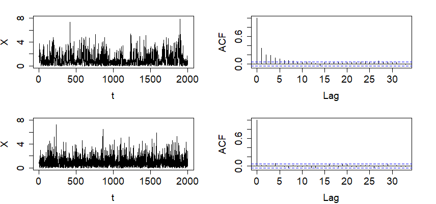
Figure 1. A correlated sample path with exponential marginal distribution and its autocorrelogram (top), a sequence of i.i.d. exponential random variables and its autocorrelogram (bottom)

Since our method produces a stationary, ergodic process with an exponential marginal distribution, we expect that the distribution of observations in a sample path, $\{X(i),i=1,2,\cdots,n\},$ for large $n,$ would be close to the exponential distribution. Figure 2 shows the fit of the observations in the correlated sample path to the exponential distribution.

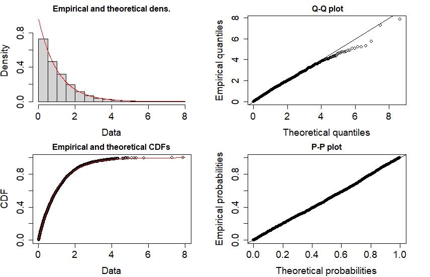
Figure 2. Comparison between the observations in the correlated sample path and exponential distribution

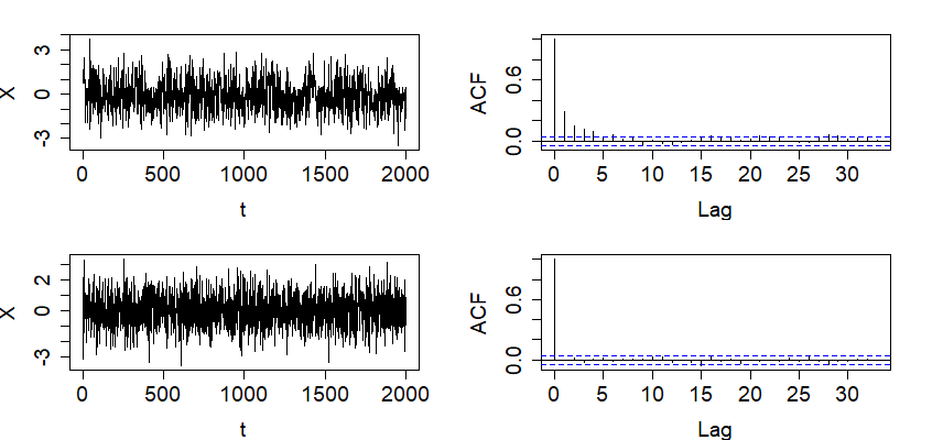
Figure 3. A correlated sample path with Gaussian marginal distribution and its autocorrelogram (top), a sequence of i.i.d. normal random variables and its autocorrelogram (bottom)

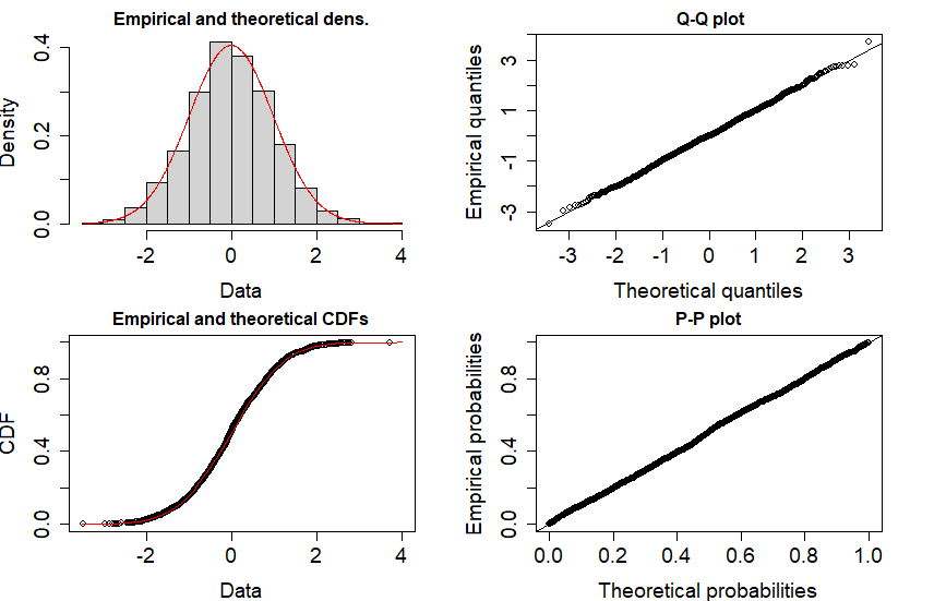
Figure 4. Comparison between the observations in the correlated sample path and standard normal distribution

We also simulate a stationary process that has one-dimensional standard normal distribution and the covariance function $cov(X(i),X(j))=c|i-j|^{2H-2},H=.7,c=.329.$ It can be easily checked by Theorem 3.1 that with GBP$(p=.3,C(i)=.12|i|^{-.6})$ and $A=(z_{.3},\infty)$, such a process can be constructed. The simulated sample path and its autocorrelogram are shown in Figure 3. For comparison purposes, we also provide the results for i.i.d. standard normal random variables on the bottom graphs in Figure 3. The observations in the correlated sample path are compared to the standard normal distribution in Figure 4. The results indicate that our sample path shows a correlation that decays as expected and marginal Gaussian distribution.

5.2. Multivariate stationary processes with a given marginal distribution

We simulate a bivariate stationary process $\mathbf{X}(t)=(X_{1}(t),X_{2}(t))^{\prime},t=1,2,\cdots,1000,$ with a Gaussian marginal distribution, $\mathbf{X}(t)\sim N({\bf 0},\begin{bmatrix}1&-.5\\ -.5&1\end{bmatrix}).$ We use GBP with $p=.258,C(i)=.2e^{-.1|i|},$ and $A=(.2,\infty)\times(-\infty,-.2).$

By Theorem 3.1, the resulting process will have variance-covariance matrix

$$corr(\mathbf{X}(i),\mathbf{X}(j))=\begin{bmatrix}.386&-.386\\ -.386&.386\end{bmatrix}e^{-.1|i-j|}$$

for $i\neq j.$

The simulated sample paths are shown on the left in Figure 5, and their respective autocorrelograms are shown on the right. The cross-correlogram is provided at the bottom in Figure 5. It is observed that the results on the correlation structures within a sample path and between sample paths are as expected.

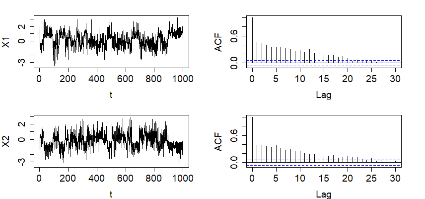
Figure 5. A bivariate stationary process with Gaussian marginal distribution

Figure 6. A bivariate stationary process with exponential marginal distribution

In Figure 6, sample paths of a bivariate stationary process with exponential marginal distribution are shown. First, a random vector of length 2 whose marginal distribution is exponential distribution is simulated with our method, i.e., $(X_{1}(t),X_{2}(t))^{\prime}\sim f(x_{1},x_{2})$ where

$$f(x_{1},x_{2})=\sum_{\ell_{1},\ell_{2}=0,1}I(x_{1}\in A_{0}^{\ell_{1}},x_{2}\in A_{0}^{\ell_{2}})\bigg{(}1+\frac{(-1)^{\ell_{1}+\ell_{2}}c_{0}}{\prod_{k=1,2}p_{0}^{\ell_{k}}(1-p_{0})^{1-\ell_{k}}}\bigg{)}{e^{-x_{1}}e^{-x_{2}}}$$

where $p_{0}=.3,c_{0}=.12,A_{0}^{1}=(-\ln{.3},\infty),A_{0}^{0}=(0,-\ln{.3}).$ With this marginal distribution, GBP $(p=.339,C(i)=.12e^{-.2|i|})$ and $A=\{(x_{1},x_{2})\in\mathbb{R}_{+}^{2}:(x_{1}>-\ln{.3},x_{2}>-\ln{.8})\text{ or }(x_{1}>-\ln{.8},x_{2}>-\ln{.3})\},$ the bivariate stationary process is simulated. Figure 6 shows its sample path, autocorrelation, and cross-correlations.

Since our construction method is not limited to continuous distributions, we also obtain a bivariate stationary process with binomial marginal distribution. In Figure 7, sample paths for a bivariate stationary process $(X_{1}(t),X_{2}(t))^{\prime},t=1,2\cdots,1000,$ with binomial marginal distribution are shown. The marginal distribution at $t$ is obtained from our method, $(X_{1}(t),X_{2}(t))^{\prime}\sim f(x_{1},x_{2})$ where

$$f(x_{1},x_{2})=\sum_{\ell_{1},\ell_{2}=0,1}I(x_{1}\in A_{0}^{\ell_{1}},x_{2}\in A_{0}^{\ell_{2}})\bigg{(}1+\frac{(-1)^{\ell_{1}+\ell_{2}}c_{0}}{\prod_{k=1,2}p_{0}^{\ell_{k}}(1-p_{0})^{1-\ell_{k}}}\bigg{)}f(x_{1})f(x_{2})$$

where $f(\cdot)$ is pmf of binomial distribution $(n=20,p=.4),p_{0}=.416,c_{0}=.12,A_{0}^{1}=\{x\in\mathbb{N}_{0}:x\leq 7\},A_{0}^{1}=\{x\in\mathbb{N}:7<x\leq 20\}.$ Applying our method again with this marginal distribution, GBP $(p=.377,C(i)=.2e^{-.2|i|})$, and $A=\{(x_{1},x_{2})\in\mathbb{N}_{0}^{2}:(x_{1}\leq 7,x_{2}\leq 9)\text{ or }(x_{1}\leq 9,x_{2}\leq 7)\},$ the bivariate stationary with binomial marginal distribution is obtained. The sample paths, autocorrelation, and cross-correlations are shown in Figure 7.

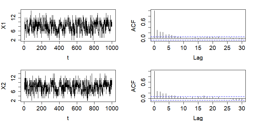
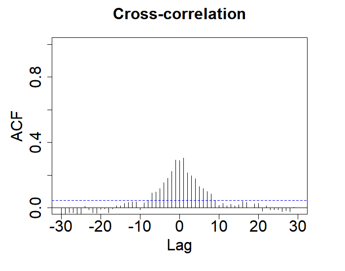
Figure 7. A bivariate stationary process with binomial marginal distribution

5.3. Stationary random fields with a given marginal distribution

We simulate a stationary random field $X(\mathbf{t}),\mathbf{t}\in\{1,2,\cdots,100\}^{2},$ with one-dimensional standard normal distribution. We use GBPs with $p_{1}=.4,C_{1}(i)=.23e^{-.4i},$ and $p_{2}=.5,C_{2}(i)=.24e^{-.5i},$ and $A^{11}=(-z_{.4},z_{.4}),A^{00}=(-z_{.25},-z_{.4})\cup(z_{.4},z_{.25}),A^{01}=(-\infty,-z_{.2})\cup(z_{.25},z_{.15}),A^{10}=(-z_{.2},-z_{.25})\cup(z_{.15},\infty).$ It is easy to see that this satisfies (4.12-4.13), therefore, the covariance is of the form in (4.14). The simulation method follows similarly. We first simulate two independent GBPs, $\{\xi_{i}^{j},i=1,\cdots,100\},$ with $(p_{j},C_{j}),j=1,2,$ using the method in Table 1, and i.i.d. standard normal random variables, $Y_{1},Y_{2},\cdots.$ For $\mathbf{t}=(1,1)^{\prime},$ let $X(\mathbf{t})=Y_{i_{\mathbf{t}}}$ where $i_{\mathbf{t}}=\min A_{\mathbf{t}},$ $A_{\mathbf{t}}=\{i:Y_{i}\in A^{\ell_{1}\ell_{2}},\ell_{j}=\xi_{t_{j}}^{j},j=1,2\}.$ For $\mathbf{t}\in\{1,\cdots,100\}^{2}/(1,1),$ let $X(\mathbf{t})=Y_{i_{\mathbf{t}}}$ where $i_{\mathbf{t}}=\min A_{\mathbf{t}}/\{i_{\mathbf{s}}:(s_{1}\in\{1,2,\cdots,100\},s_{2}<t_{2})\text{ or }(s_{1}<t_{2},s_{2}=t_{2})\}.$

The simulated random field $X(\mathbf{t})$ is shown on the top left in Figure 8, and its estimated correlation,

$$\sum_{\mathbf{t}-\mathbf{t}^{\prime}={\mathbf{s}}}\frac{(X(\mathbf{t})-\bar{X})(X(\mathbf{t}^{\prime})-\bar{X})}{|N_{\mathbf{s}}|}$$

for $\mathbf{s}\in\{-25,\cdots,-1,0,1,\cdots,25\}^{2}$, where $N_{\mathbf{s}}=\{(\mathbf{t},\mathbf{t}^{\prime}):\mathbf{t},\mathbf{t}^{\prime}\in\{1,2,\cdots,100\}^{2},\mathbf{t}-\mathbf{t}^{\prime}=\mathbf{s}\},$ on the top right in Figure 8.

We also simulate a random field with one-dimensional standard normal distribution, with GBPs $(p_{1}=.5,C_{1}(i)=.23e^{-.4|i|},$ $p_{2}=.0.549,C_{2}(i)=.24e^{-.5|i|}),$ and $A^{10}=(.5,1.386),A^{01}=\mathbb{R}_{+}/A^{10},A^{11}=\{-x:x\in A^{01}\},A^{00}=\{-x:x\in A^{10}\}.$ It is easy to check that (4.9-4.10) are satisfied, therefore, the resulting random field will have the covariance of the form in (4.11). The simulated random field and its estimated correlation are shown in the bottom graphs of Figure 8.

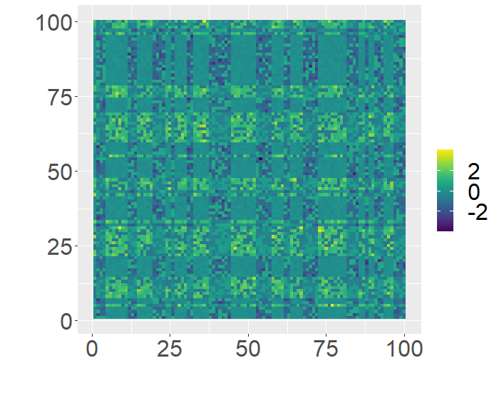
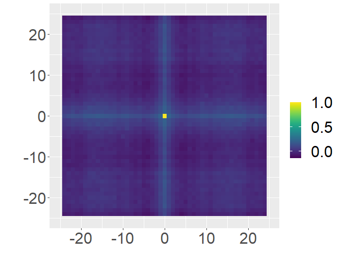
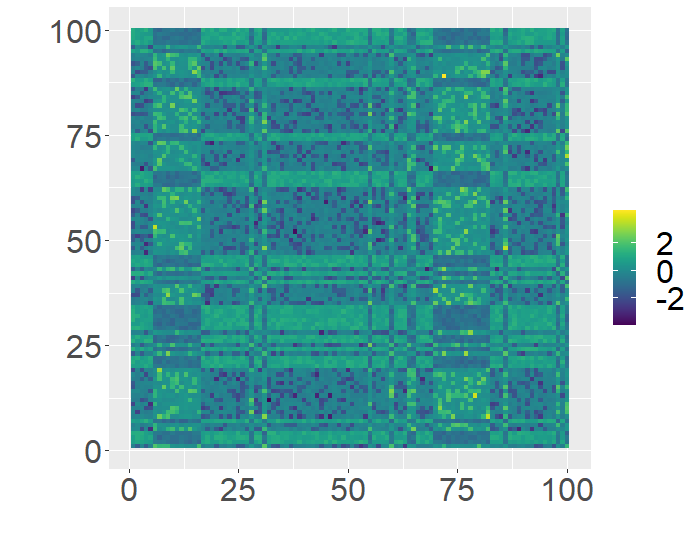
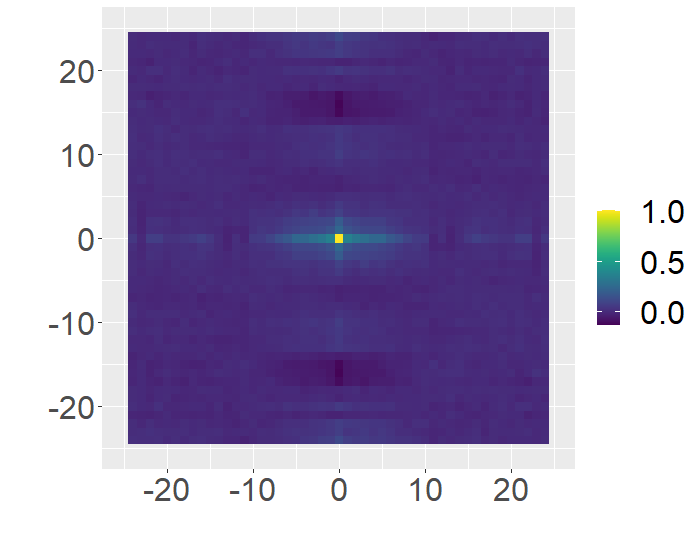
Figure 8. Random fields with one-dimensional Gaussian marginal distribution and its correlation

6. Concluding Remarks

We proposed a new method to construct a stationary process/random field with any given one-dimensional distribution and a given covariance function that is decreasing and convex. The method utilized a generalized Bernoulli process (GBP), a stationary binary sequence that can have a flexible covariance structure, as a latent process. For a stationary process, a random variable was generated from one of two disjoint sets in the marginal distribution which is chosen from the state of GBP at each time. The method was easily extended to a random field where several GBPs were used as latent processes and a random variable was generated from one of several disjoint sets of marginal distribution that is chosen from the states of GBPs.

For future work, it would be interesting if GBP is further extended to include more broad covariance functions that can show sinuous shapes, which will enable the construction of a stationary process/random field with a broader covariance structure with any given marginal distribution. Also, instead of using a stationary binary sequence that has two states, one can use a stationary process with several states as a latent process to induce various covariance structures of a stationary process/random field.

7. Proofs

Lemma 7.1.

Under Assumption 2.3, $D(A,\{i\})=L(A)-L(A\cup\{i\})>0$ for any $A,\{i\}\subset\mathbb{N},i\notin A.$

Proof.

If $A=\emptyset,$ $D(A,\{i\})=1-p>0.$ If $A=\{i^{\prime}\},D(A,\{i\})=p-p(p+c(|i^{\prime}-i|))>0$ since $p+c(x)<1$ for any $x\in\mathbb{N}.$

Let $|A|=2.$ We will show that $D(\{i_{0},i_{2}\},\{i_{1}\})=L(\{i_{0},i_{2}\})-L(\{i_{0},i_{1},i_{2}\})>0$ for any $i_{0},i_{1},i_{2}\in\mathbb{N}.$

If $\max\{i_{0},i_{2}\}<i_{1}$ or $\min\{i_{0},i_{2}\}>i_{1},$ the result easily follows since

$$L(\{i_{0},i_{1},i_{2}\})=\begin{dcases}L(\{i_{0},i_{2}\})(p+c(|i_{1}-\min\{i_{0},i_{2}\}|))&\text{if }i_{1}<\min\{i_{0},i_{2}\},\\ L(\{i_{0},i_{2}\})(p+c(|i_{1}-\max\{i_{0},i_{2}\}|))&\text{if }i_{1}>\max\{i_{0},i_{2}\}.\end{dcases}$$

Now, assume $i_{0}<i_{1}<i_{2}.$ We need to show that

$$\frac{L(\{i_{0},i_{2}\})}{L(\{i_{0},i_{1},i_{2}\})}=\frac{p+c(x+a)}{(p+c(x))(p+c(a))}>1,$$

for any $x=i_{1}-i_{0},a=i_{2}-i_{1}\in\mathbb{N}.$ Since $p+c(x)$ is a convex function, it follows that $(p+c(x+a))/(p+c(x))$ is an increasing function of $x$ for any $a.$ Therefore,

$$\frac{p+c(x+a)}{(p+c(x))(p+c(a))}\geq\frac{p+c(1+a)}{(p+c(1))(p+c(a))}\geq\frac{p+c(2)}{(p+c(1))(p+c(1))}>1,$$

where we used the fact that $(p+c(1+a))/(p+c(a))$ is an increasing function of $a$ and Assumption 2.3.

For $|A|>2,$ it is derived in the same way as $|A|=2.$ If $\max A<i$ or $\min A>i,$

$$L(A\cup\{i\})=\begin{dcases}L(A)(p+c(|i-\min A|))&\text{if }i<\min A,\\ L(A)(p+c(|i-\max A|))&\text{if }i>\max A,\end{dcases}$$

therefore, $D(A,\{i\})>0.$ If $\min A<i<\max A,$ let $i^{*}=min\{j:j\in A,j>i\}$, $i_{*}=max\{j:j\in A,j<i\}.$ Then,

$$\frac{L(A)}{L(A\cup\{i\})}=\frac{L(\{i_{*},i^{*}\})}{L(\{i_{*},i,i^{*}\})}>1.$$

∎

Proof of Theorem 2.6.
We will prove for any disjoint sets $A_{1}\sqcup A_{0}\subset\mathbb{Z}$

$$D(A_{1},A_{0})>0$$ (7.1)

by mathematical induction. If $A_{0}=\emptyset,D(A_{1},A_{0})=L(A_{1})>0.$ Assume $A_{0}\neq\emptyset.$

If $|A_{0}|=1,$ $D(A_{1},A_{0})=L(A_{1})-L(A_{1}\cup\ A_{0})>0,$ by Lemma 7.1. Assume (7.1) holds with $|A_{0}|\leq m.$ We will show that (7.1) holds when $|A_{0}|=m+1.$ Let $A_{0}=\{i_{0}^{\prime},i_{1}^{\prime},i_{2}^{\prime},\cdots,i_{m}^{\prime}\}$ with $i_{0}^{\prime}<i_{1}^{\prime}<i_{2}^{\prime}<\cdots<i_{m}^{\prime}.$ By Lemma 5.1 in [5], it is enough to show that

$$D(A_{1},A_{0}/\{i_{m}^{\prime}\})>D(A_{1}\cup\{i_{m}^{\prime}\},A_{0}/\{i_{m}^{\prime}\}).$$

By (7.1),

$$\frac{D(A_{1},A_{0}/\{i_{m}^{\prime}\})}{D(A_{1}\cup\{i_{m}^{\prime}\},A_{0}/\{i_{m}^{\prime}\})}=\frac{a_{0}-a_{1}-a_{2}-a_{3}\cdots-a_{m-1}}{a_{0}^{\prime}-a_{1}^{\prime}-a_{2}^{\prime}-a_{3}^{\prime}\cdots-a_{m-1}^{\prime}},$$ (7.2)

where

$${a_{j}}=\begin{dcases}{D(A_{1}\cup\{i_{j}^{\prime}\},\{i_{0}^{\prime},i_{1}^{\prime},\cdots,i_{j-1}^{\prime}\})}&\text{for }j=1,\cdots,m-1,\\ {D(A_{1},\{i_{0}^{\prime}\})}&\text{for }j=0,\end{dcases}$$

and

$${a_{j}^{\prime}}=\begin{dcases}{D(A_{1}\cup\{i_{j}^{\prime},i_{m}^{\prime}\},\{i_{0}^{\prime},i_{1}^{\prime},\cdots,i_{j-1}^{\prime}\})}&\text{for }j=1,\cdots,m-1,\\ {D(A_{1}\cup\{i_{m}^{\prime}\},\{i_{0}^{\prime}\})},&\text{for }j=0.\end{dcases}$$

We will apply Lemma 5.2 i) in [5] to show that $(7.2)>1.$ Note that $a_{0}-a_{1}-\cdots-a_{j}>0$ and $a_{0}^{\prime}-a_{1}^{\prime}-\cdots-a_{j}^{\prime}>0$ for $j=0,1,\cdots,m-1,$ by the earlier assumption that (7.1) holds for $|A_{0}|\leq m.$

Define $i_{j}^{*}=\max\{i_{j}^{\prime},i:i\in A_{1},i<i_{m}^{\prime}\}.$ Note that $i_{j}^{*}$ is non-decreasing as $j$ goes from 1 to $m-1$. If $\max A_{1}>i_{m}^{\prime}$, define $i^{*}=\min\{i:i\in A_{1},i>i_{m}^{\prime}\}.$ For $j=1,\cdots,m-1,$

$$\frac{a_{j}}{a_{j}^{\prime}}=\frac{D(A_{1}\cup\{i_{j}^{\prime}\},\{i_{0}^{\prime},i_{1}^{\prime},\cdots,i_{j-1}^{\prime}\})}{D(A_{1}\cup\{i_{j}^{\prime},i_{m}^{\prime}\},\{i_{0}^{\prime},i_{1}^{\prime},\cdots,i_{j-1}^{\prime}\})}$$

$$=\begin{dcases}\frac{p+c(i^{*}-i_{j}^{*})}{(p+c(i_{m}^{\prime}-i_{j}^{*}))(p+c(i^{*}-i_{m}^{\prime}))}&\text{ if }\max A_{1}>i_{m}^{\prime},\\ \frac{1}{p+c(i_{m}^{\prime}-i_{j}^{*})}&\text{ if }\max A_{1}<i_{m}^{\prime},\\ \frac{1}{p+c(i_{m}^{\prime}-i_{j}^{\prime})}&\text{ if }A_{1}=\emptyset,\end{dcases}$$ (7.3)

which is non-increasing as $j$ goes from 1 to $m-1,$ since $p+c(x)$ is a decreasing function and $(p+c(x+a))/(p+c(x))$ is also a decreasing functions of $x$ for any $a>0.$

Also,

$$\frac{a_{0}}{a_{0}^{\prime}}=\frac{D(A_{1},\{i_{0}^{\prime}\})}{D(A_{1}\cup\{i_{m}^{\prime}\},\{i_{0}^{\prime}\})}=\frac{L(A_{1})-L(A_{1}\cup\{i_{0}^{\prime}\})}{L(A_{1}\cup\{i_{m}^{\prime}\})-L(A_{1}\cup\{i_{0}^{\prime},i_{m}^{\prime}\})}$$

with

$$\frac{L(A_{1})}{L(A_{1}\cup\{i_{m}^{\prime}\})}=\begin{dcases}\frac{1}{p+c(i^{*}-i_{m}^{\prime})}&\text{ if }\min A_{1}>i_{m}^{\prime},\\ \frac{1}{p+c(i_{m}^{\prime}-i_{*})}&\text{ if }\max A_{1}<i_{m}^{\prime},\\ \frac{p+c(i^{*}-i_{*})}{(p+c(i^{*}-i_{m}^{\prime}))(p+c(i_{m}^{\prime}-i_{*}))}&\text{ if }\min A_{1}<i_{m}^{\prime}<\max A_{1},\\ 1/p&\text{ if }A_{1}=\emptyset,\end{dcases}$$

where $i_{*}=\max\{i:i\in A_{1},i<i_{m}^{\prime}\}$ if $\min A_{1}<i_{m}^{\prime},$ and

$$\frac{L(A_{1}\cup\{i_{0}^{\prime}\})}{L(A_{1}\cup\{i_{0}^{\prime},i_{m}^{\prime}\})}=(7.3)$$

with $j=0.$ Since $i_{*}\leq i_{0}^{*}\leq i_{1}^{*}\leq i_{2}^{*}\leq\cdots\leq i_{m-1}^{*},$

$$\frac{L(A_{1})}{L(A_{1}\cup\{i_{m}^{\prime}\})}\geq\frac{L(A_{1}\cup\{i_{0}^{\prime}\})}{L(A_{1}\cup\{i_{0}^{\prime},i_{m}^{\prime}\})}\geq\frac{a_{1}}{a_{1}^{\prime}}\geq\frac{a_{2}}{a_{2}^{\prime}}\geq\cdots\geq\frac{a_{m-1}}{a_{m-1}^{\prime}}$$

therefore, by Lemma 5.2 i) in [5],

$$(7.3)\geq\frac{L(A_{1})}{L(A_{1}\cup\{i_{m}^{\prime}\})}.$$

The result follows as $\frac{L(A_{1})}{L(A_{1}\cup\{i_{m}^{\prime}\})}>1$ by Lemma 7.1. ∎

Proof of Theorem 3.1.
Note that for any set $B\subset\mathbb{R}^{d}$ and any $i\in\mathbb{Z},$

$$P(\mathbf{X}(i)\in B) =P(\mathbf{X}^{A}(i)\in B)P(\xi_{i}=1)+P(\mathbf{X}^{A^{c}}(i)\in B)P(\xi_{i}=0)$$

$$=\frac{\int_{A\cap B}f({\bf x})d{\bf x}}{p}p+\frac{\int_{A^{c}\cap B}f({\bf x})d{\bf x}}{1-p}(1-p)=\int_{B}f({\bf x})d{\bf x}.$$

Also,

$$P(\cap_{j=1}^{k}\{\mathbf{X}({i_{j}})\in B_{j}\})=P(\cap_{j=1}^{k}\{\mathbf{X}({i_{j}+\ell})\in B_{j})$$

for any $k\in\mathbb{N},\ell,i_{1},i_{2},\cdots,i_{k}\in\mathbb{Z},$ since $\{\xi_{i},i\in\mathbb{Z}\}$ is stationary, $\{\mathbf{X}^{A}(i),i\in\mathbb{Z}\}$ and $\{\mathbf{X}^{A^{c}}(i),i\in\mathbb{Z}\}$ are i.i.d., and the three sequences of random variables are independent of each other. Therefore, $\{\mathbf{X}(i),i\in\mathbb{Z}\}$ is a stationary process with marginal pdf $f.$ Without loss of generality, let $\mu=0.$ If $\mu\neq 0,$ one can use $\mathbf{X}(i)-\mu=(\mathbf{X}^{A}(i)-\mu)I_{\{\xi_{i}=1\}}+(\mathbf{X}^{A^{c}}(i)-\mu)I_{\{\xi_{i}=0\}}.$ Since

$$E(X_{k}(i)X_{\ell}(j)) =\sum_{u,v=0,1}E(X_{k}^{A^{u}})E(X_{\ell}^{A^{v}})E(I_{\{\xi_{i}=u\}}I_{\{\xi_{j}=v\}})$$

$$=\sum_{u,v=0,1}\frac{\int_{A^{u}}x_{k}f({\bf x})d{\bf x}\int_{A^{v}}x_{\ell}f({\bf x})d{\bf x}\Big{(}p^{u+v}(1-p)^{2-u-v}+(-1)^{u+v}C(|i-j|)\Big{)}}{p^{u+v}(1-p)^{2-u-v}}$$

$$=\frac{d_{k}d_{\ell}}{p^{2}(1-p)^{2}}C(|i-j|),$$

where $A^{0}=A^{c},A^{1}=A$, and $d_{k}=\int_{A}x_{k}f({\bf x})d{\bf x}$, the result follows. ∎

Proof of Proposition 3.3.
We can show that

$$P(\{\mathbf{X}(i)\in B_{1}\}\cap\{\mathbf{X}(j)\in B_{2}\})=\Big{(}\prod_{k=1,2}P(\mathbf{X}^{A}(i)\in B_{k})\Big{)}P(\{\xi_{i}=1\}\cap\{\xi_{j}=1\})$$

$$+\Big{(}P(\mathbf{X}^{A}(i)\in B_{1})P(\mathbf{X}^{A^{c}}(i)\in B_{2})+P(\mathbf{X}^{A}(i)\in B_{2})P(\mathbf{X}^{A^{c}}(i)\in B_{1})\Big{)}P(\{\xi_{i}=0\}\cap\{\xi_{j}=1\})$$

$$+\Big{(}\prod_{k=1,2}P(\mathbf{X}^{A^{c}}(i)\in B_{k})\Big{)}P(\{\xi_{i}=0\}\cap\{\xi_{j}=0\})$$

$$=\Bigg{(}\prod_{k=1,2}\frac{\int_{A\cap B_{k}}f({\bf x})d{\bf x}}{p}\Bigg{)}p(p+C^{*}(|i-j|))$$

$$+\bigg{(}\frac{\int_{A\cap B_{1}}f({\bf x})d{\bf x}\int_{A^{c}\cap B_{2}}f({\bf x})d{\bf x}}{p(1-p)}+\frac{\int_{A\cap B_{2}}f({\bf x})d{\bf x}\int_{A^{c}\cap B_{1}}f({\bf x})d{\bf x}}{p(1-p)}\Bigg{)}p(1-p-C^{*}(|i-j|))$$

$$+\Bigg{(}\prod_{k=1,2}\frac{\int_{A^{c}\cap B_{k}}f({\bf x})d{\bf x}}{1-p}\Bigg{)}((1-p)^{2}+pC^{*}(|i-j|))$$

$$=\prod_{k=1,2}\Bigg{(}\int_{A\cap B_{k}}f({\bf x})d{\bf x}+\int_{A^{c}\cap B_{k}}f({\bf x})d{\bf x}\Bigg{)}+pC^{*}(|i-j|)\prod_{k=1,2}\Bigg{(}\frac{\int_{A\cap B_{k}}f({\bf x})d{\bf x}}{p}-\frac{\int_{A^{c}\cap B_{k}}f({\bf x})d{\bf x}}{1-p}\Bigg{)}.$$

Since $P(\mathbf{X}(i)\in B_{k})=\int_{A\cap B_{k}}f({\bf x})d{\bf x}+\int_{A^{c}\cap B_{k}}f({\bf x})d{\bf x},$ for $k=1,2,$ the result follows. ∎

Proof of Theorem 3.6.
Here, we abuse the notations and understand $L^{*}(K),D(B,F)$ for $K,B,F\subset\mathbb{Z}$ as $L^{*}(\{i_{j}:j\in K\})$ and $D(\{i_{j}:j\in B\},\{i_{j}:j\in F\})$, respectively. By (2.1),

$$E(e^{i\sum_{j=1,2,\cdots,k}\theta_{j}\mathbf{X}(i_{j})})=\sum_{\begin{subarray}{c}B\cup F=\{1,2,\cdots,k\}\\ B\cap F=\emptyset\end{subarray}}\prod_{i\in B}E(e^{{\rm i}\theta_{i}^{\prime}\mathbf{X}^{A}})\prod_{j\in F}E(e^{{\rm i}\theta_{j}^{\prime}\mathbf{X}^{A^{c}}})pD(B,F)$$

$$=(G)+(H)$$

where (G)=terms that does not include $L^{*}$, and (H)=terms that include $L^{*}(K)$.

In $pD(B,F),$ the terms that do not include $L^{*}$ are by the definition of the operations $D,L,$

$$\sum_{j=0}^{|F|}\sum_{\begin{subarray}{c}F^{\prime}\subset F\\ |F^{\prime}|=j\end{subarray}}(-p)^{j}p^{|B|}=p^{|B|}(1-p)^{|F|},$$

therefore,

$$(G)= \sum_{\begin{subarray}{c}B\cup F=\{1,2,\cdots,k\}\\ B\cap F=\emptyset\end{subarray}}\prod_{i\in B}E(e^{{\rm i}\mathbf{t}_{i}^{\prime}\mathbf{X}^{A}})\prod_{j\in F}E(e^{{\rm i}\mathbf{t}_{j}^{\prime}\mathbf{X}^{A^{c}}})p^{|B|}(1-p)^{|F|}=\prod_{j=1}^{k}\Big{(}E(e^{{\rm i}\mathbf{t}_{j}^{\prime}\mathbf{X}^{A}})p+E(e^{{\rm i}\mathbf{t}_{j}^{\prime}\mathbf{X}^{A^{c}}})(1-p)\Big{)}$$

$$=\prod_{j=1}^{k}E(e^{{\rm i}\mathbf{t}_{j}^{\prime}\mathbf{X}}).$$

The terms that include $L^{*}(K)$ in $pD(B,F)$ are

$$\sum_{\begin{subarray}{c}K\subset[k]\\ |K|\geq 2\end{subarray}}\sum_{F^{\prime}\subset F}\sum_{\begin{subarray}{c}K\subset(B\cup F^{\prime})\\ W\in Q_{K}\\ W^{\circ}\cap(B\cup F^{\prime})=\emptyset\end{subarray}}(-1)^{|F^{\prime}|}p^{|B|+|F^{\prime}|-|K|}L^{*}(W)$$

where $W^{\circ}=\sqcup K_{i}^{\circ}$ for $W=\{K_{i},i=1,2,\cdots,|W|\},$ therefore,

$$(H)= \sum_{\begin{subarray}{c}K\subset[k]\\ |K|\geq 2\\ W\in Q_{K}\end{subarray}}\prod_{j\in W^{\circ}}E(e^{{\rm i}\theta_{j}^{\prime}\mathbf{X}^{A^{c}}})\sum_{\begin{subarray}{c}B\cup F=\{1,\cdots,k\}/W^{\circ}\\ B\cap F=\emptyset\end{subarray}}\prod_{i\in B}E(e^{{\rm i}\theta_{i}^{\prime}\mathbf{X}^{A}})\prod_{\ell\in F}E(e^{{\rm i}\mathbf{t}_{\ell}^{\prime}\mathbf{X}^{A^{c}}})$$

$$\sum_{\begin{subarray}{c}F^{\prime}\subset F\\ K\cap B^{c}\subset F^{\prime}\end{subarray}}p^{|B|}(-p)^{|K\cap B^{c}|}(-p)^{|F^{\prime}|-|K\cap B^{c}|}p^{-|K|}L^{*}(W)$$

$$=\sum_{\begin{subarray}{c}K\subset[k]\\ |K|\geq 2\\ W\in Q_{K}\end{subarray}}\prod_{j\in W^{\circ}}E(e^{{\rm i}\theta_{j}^{\prime}\mathbf{X}^{A^{c}}})\sum_{\begin{subarray}{c}B\cup F=\{1,\cdots,k\}/W^{\circ}\\ B\cap F=\emptyset\end{subarray}}\prod_{i\in B}E(e^{{\rm i}\theta_{i}^{\prime}\mathbf{X}^{A}})\prod_{\ell\in F}E(e^{{\rm i}\theta_{\ell}^{\prime}\mathbf{X}^{A^{c}}})$$

$$p^{|B|}(-p)^{|K\cap B^{c}|}(1-p)^{|F|-|K\cap B^{c}|}p^{-|K|}L^{*}(W)$$

$$=\sum_{\begin{subarray}{c}K\subset[k]\\ |K|\geq 2\\ W\in Q_{K}\end{subarray}}\prod_{j\in W^{\circ}}E(e^{{\rm i}\theta_{j}^{\prime}\mathbf{X}^{A^{c}}})\sum_{\begin{subarray}{c}B\cup F=\{1,\cdots,k\}/W^{\circ}\\ B\cap F=\emptyset\end{subarray}}\prod_{i\in B}E(e^{{\rm i}\theta_{i}^{\prime}\mathbf{X}^{A}})\prod_{\ell\in F}E(e^{{\rm i}\theta_{\ell}^{\prime}\mathbf{X}^{A^{c}}})$$

$$p^{|B\cap K^{c}|}(-1)^{|K\cap B^{c}|}(1-p)^{|F|-|K\cap B^{c}|}L^{*}(W)$$

$$=\sum_{\begin{subarray}{c}K\subset[k]\\ |K|\geq 2\\ W\in Q_{K}\end{subarray}}\prod_{j\in W^{\circ}}E(e^{{\rm i}\mathbf{t}_{j}^{\prime}\mathbf{X}^{A^{c}}})\prod_{i\in K}(E(e^{{\rm i}\theta_{i}^{\prime}\mathbf{X}^{A}})-E(e^{{\rm i}\theta_{i}^{\prime}\mathbf{X}^{A^{c}}}))$$

$$\prod_{\ell\in\{1,\cdots,k\}/(W^{\circ}\cup K)}(pE(e^{{\rm i}\theta_{\ell}^{\prime}\mathbf{X}^{A}})+(1-p)E(e^{{\rm i}\theta_{\ell}^{\prime}\mathbf{X}^{A^{c}}}))L^{*}(W).$$

∎

Proof of Theorem 4.1.
It is easy to see that $\{\mathbf{X}(\mathbf{t}),\mathbf{t}\in\mathbb{Z}^{2}\}$ is a stationary random field with marginal pdf $f.$ Also,

$$E(\mathbf{X}(\mathbf{t})\mathbf{X}(\mathbf{s})^{\prime}) =\sum_{\ell_{1},\ell_{2},\ell_{1}^{\prime},\ell_{2}^{\prime}=0,1}\mathbf{d}_{\ell_{1}\ell_{2}}\mathbf{d}_{\ell_{1}^{\prime}\ell_{2}^{\prime}}^{\prime}P(\{\xi_{t_{1}}^{1}=\ell_{1}\}\cap\{\xi_{s_{1}}^{1}=\ell_{1}^{\prime}\})P({\{\xi_{t_{2}}^{2}=\ell_{2}\}\cap\{\xi_{s_{2}}^{2}=\ell_{2}^{\prime}\}})$$

$$=\sum_{i,i^{\prime},j,j^{\prime}=0,1}\mathbf{d}_{ij}\mathbf{d}_{i^{\prime}j^{\prime}}^{\prime}\Big{(}p_{1}^{i+i^{\prime}}(1-p_{1})^{2-i-i^{\prime}}+(-1)^{i+i^{\prime}}C_{1}(|t_{1}-s_{1}|)\Big{)}$$

$$\times\Big{(}p_{2}^{j+j^{\prime}}(1-p_{2})^{2-j-j^{\prime}}+(-1)^{j+j^{\prime}}C_{2}(|t_{2}-s_{2}|)\Big{)}$$

$$=\Big{(}\sum_{\ell_{1},\ell_{2}=0,1}\mathbf{d}_{\ell_{1}\ell_{2}}\prod_{k=1,2}p_{k}^{\ell_{k}}(1-p_{k})^{1-\ell_{k}}\Big{)}\Big{(}\sum_{\ell_{1},\ell_{2}=0,1}\mathbf{d}_{\ell_{1}\ell_{2}}\prod_{k=1,2}p_{k}^{\ell_{k}}(1-p_{k})^{1-\ell_{k}}\Big{)}^{\prime}$$

$$+p_{1}p_{2}C_{1}^{*}(|t_{1}-s_{1}|)C_{2}^{*}(|t_{2}-s_{2}|){\bf v}_{0}{\bf v}_{0}^{\prime}+p_{1}C_{1}^{*}(|t_{1}-s_{1}|){\bf v_{1}}{\bf v_{1}}^{\prime}$$

$$+p_{2}C_{2}^{*}(|t_{2}-s_{2}|){\bf v_{2}}{\bf v_{2}}^{\prime}$$

where

$$\mathbf{d}_{\ell_{1}\ell_{2}} =E(\mathbf{X}^{A^{\ell_{1}\ell_{2}}}(\mathbf{t}))=\Bigg{(}\frac{\int_{A^{\ell_{1}\ell_{2}}}x_{1}f(\mathbf{x})d\mathbf{x}}{\prod_{k=1,2}p_{k}^{\ell_{k}}(1-p_{k})^{1-\ell_{k}}},\cdots,\frac{\int_{A^{\ell_{1}\ell_{2}}}x_{d}f(\mathbf{x})d\mathbf{x}}{\prod_{k=1,2}p_{k}^{\ell_{k}}(1-p_{k})^{1-\ell_{k}}}\Bigg{)}^{\prime},$$

for $\ell_{1},\ell_{2}=0,1,$ and ${\bf v_{0}}=\mathbf{d}_{10}+\mathbf{d}_{01}-\mathbf{d}_{11}-\mathbf{d}_{00},$ ${\bf v_{1}}=p_{2}(\mathbf{d}_{11}-\mathbf{d}_{01})+(1-p_{2})(\mathbf{d}_{10}-\mathbf{d}_{00}),$ ${\bf v_{2}}=p_{1}(\mathbf{d}_{11}-\mathbf{d}_{10})+(1-p_{1})(\mathbf{d}_{01}-\mathbf{d}_{00}).$ Since

$$\sum_{\ell_{1},\ell_{2}=0,1}\mathbf{d}_{\ell_{1}\ell_{2}}\prod_{k=1,2}p_{k}^{\ell_{k}}(1-p_{k})^{1-\ell_{k}}=E(\mathbf{X}(\mathbf{t})),$$

the result follows. For other cases, the results are derived similarly. ∎

Proof of Theorem 4.4.
First, assume that $t_{j}\neq s_{j}$ for all $j=1,2,\cdots,n,$ i.e., $O_{(\mathbf{t}-\mathbf{s})}=\emptyset.$ Then,

$$E(\mathbf{X}({\bf t})\mathbf{X}({\bf s})^{\prime})=\sum_{\begin{subarray}{c}\ell_{1},\ell_{2},\cdots,\ell_{n}=0,1\\ \ell_{1}^{\prime},\ell_{2}^{\prime},\cdots,\ell_{n}^{\prime}=0,1\end{subarray}}E\big{(}\mathbf{X}^{A^{\ell_{1}\cdots\ell_{n}}}\big{)}E\big{(}\mathbf{X}^{A^{\ell_{1}^{\prime}\cdots\ell_{n}^{\prime}}}\big{)}^{\prime}\prod_{j\in[n]}P(\xi_{t_{j}}^{j}=\ell_{j},\xi_{s_{j}}^{j}=\ell_{j}^{\prime}).$$ (7.4)

Note that $P(\xi_{t_{j}}^{j}=\ell_{j},\xi_{s_{j}}^{j}=\ell_{j}^{\prime})=p_{j}^{\ell_{j}}(1-p_{j})^{1-\ell_{j}}p_{j}^{\ell_{j}^{\prime}}(1-p_{j})^{1-\ell_{j}^{\prime}}+(-1)^{2-(\ell_{j}+\ell_{j}^{\prime})}C_{j}(|t_{j}-s_{j}|)$ by (2.1), which leads to

$$(7.4) =\Bigg{(}\sum_{\ell_{1},\cdots,\ell_{n}=0,1}E\big{(}\mathbf{X}^{A^{\ell_{1}\cdots\ell_{n}}}\big{)}\prod_{j\in[n]}p_{j}^{\ell_{j}}(1-p_{j})^{1-\ell_{j}}\Bigg{)}\Bigg{(}\sum_{\ell_{1}^{\prime},\cdots,\ell_{n}^{\prime}=0,1}E\big{(}\mathbf{X}^{A^{\ell_{1}^{\prime}\cdots\ell_{n}^{\prime}}}\big{)}^{\prime}\prod_{j\in[n]}p_{j}^{\ell_{j}^{\prime}}(1-p_{j})^{1-\ell_{j}^{\prime}}\Bigg{)}$$

$$+\sum_{\begin{subarray}{c}K\subset[n]\\ K\neq\emptyset\end{subarray}}\prod_{k\in K}C_{k}(|t_{k}-s_{k}|)\Bigg{(}\sum_{\ell_{1},\cdots,\ell_{n}=0,1}(-1)^{|K|-\sum_{i\in K}\ell_{i}}E\big{(}\mathbf{X}^{A^{\ell_{1}\cdots\ell_{n}}}\big{)}\prod_{j\in[n]/K}p_{j}^{\ell_{j}}(1-p_{j})^{1-\ell_{j}}\Bigg{)}$$

$$\Bigg{(}\sum_{\ell_{1}^{\prime},\cdots,\ell_{n}^{\prime}=0,1}(-1)^{|K|-\sum_{i\in K}\ell_{i}^{\prime}}E\big{(}\mathbf{X}^{A^{\ell_{1}^{\prime}\cdots\ell_{n}^{\prime}}}\big{)}^{\prime}\prod_{j\in[n]/K}p_{j}^{\ell_{j}^{\prime}}(1-p_{j})^{1-\ell_{j}^{\prime}}\Bigg{)}.$$

Since

$$E(\mathbf{X})=\sum_{\ell_{1},\cdots,\ell_{n}=0,1}E\big{(}\mathbf{X}^{A^{\ell_{1}\cdots\ell_{n}}}\big{)}\prod_{j\in[n]}p_{j}^{\ell_{j}}(1-p_{j})^{1-\ell_{j}},$$

the result follows.

If $O_{(\mathbf{t}-\mathbf{s})}\neq\emptyset,$ (7.4) becomes

$$\sum_{\begin{subarray}{c}\ell_{j^{\prime}}=0,1\\ j^{\prime}\in O_{(\mathbf{t}-\mathbf{s})}\end{subarray}}\Bigg{(}\prod_{j^{\prime}\in O_{(\mathbf{t}-\mathbf{s})}}P(\xi_{t_{j^{\prime}}}^{j^{\prime}}=\ell_{j^{\prime}})\Bigg{)}\sum_{\begin{subarray}{c}\ell_{j},\ell_{j}^{\prime}=0,1\\ j\in[n]/O_{(\mathbf{t}-\mathbf{s})}\end{subarray}}E\big{(}\mathbf{X}^{A^{\ell_{1}\cdots\ell_{n}}}\big{)}E\big{(}\mathbf{X}^{A^{\ell_{1}^{\prime}\cdots\ell_{n}^{\prime}}}\big{)}^{\prime}\prod_{i\in[n]/O_{(\mathbf{t}-\mathbf{s})}}P(\xi_{t_{i}}^{i}=\ell_{i},\xi_{s_{i}}^{i}=\ell_{i}^{\prime}),$$

and as in the previous case, we can show that

$$\sum_{\begin{subarray}{c}\ell_{j},\ell_{j}^{\prime}=0,1\\ j\in[n]/O_{(\mathbf{t}-\mathbf{s})}\end{subarray}}E\big{(}\mathbf{X}^{A^{\ell_{1}\cdots\ell_{n}}}\big{)}E\big{(}\mathbf{X}^{A^{\ell_{1}^{\prime}\cdots\ell_{n}^{\prime}}}\big{)}^{\prime}\prod_{i\in[n]/O_{(\mathbf{t}-\mathbf{s})}}P(\xi_{t_{i}}^{i}=\ell_{i},\xi_{s_{i}}^{i}=\ell_{i}^{\prime})$$

$$={\bf qq^{\prime}}+\sum_{\begin{subarray}{c}K\subset[n]/O_{(\mathbf{t}-\mathbf{s})}\\ K\neq\emptyset\end{subarray}}\bigg{(}\prod_{k\in K}C_{k}(|t_{k}-s_{k}|)\bigg{)}{\bf vv^{\prime}}$$

where

$${\bf q} =\sum_{\begin{subarray}{c}\ell_{j}=0,1\\ j\in[n]/O_{(\mathbf{t}-\mathbf{s})}\end{subarray}}E\big{(}\mathbf{X}^{A^{\ell_{1}\cdots\ell_{n}}}\big{)}\prod_{i\in[n]/O_{(\mathbf{t}-\mathbf{s})}}p_{i}^{\ell_{i}}(1-p_{i})^{1-\ell_{i}}$$

$${\bf v} =\sum_{\begin{subarray}{c}\ell_{i^{\prime}}=0,1\\ i^{\prime}\in[n]/O_{(\mathbf{t}-\mathbf{s})}\end{subarray}}(-1)^{|K|-\sum_{i\in K}\ell_{i}}E\big{(}\mathbf{X}^{A^{\ell_{1}\cdots\ell_{n}}}\big{)}\prod_{j\in[n]/(K\cup O_{(\mathbf{t}-\mathbf{s})})}p_{j}^{\ell_{j}}(1-p_{j})^{1-\ell_{j}},$$

from which the result follows. ∎

Proof of Proposition 4.5.
For $k\subset K^{\prime},K\neq\emptyset,$ we have from (4.7)

$${\bf m}_{K}=\sum_{\begin{subarray}{c}\ell_{j}=0,1\\ j\in K/O_{(\mathbf{t}-\mathbf{s})}\end{subarray}}(-1)^{O^{K/O_{(\mathbf{t}-\mathbf{s})}}}\frac{\int_{A(\{\ell_{i},i\in K\cup O_{(\mathbf{t}-\mathbf{s})}\})}x_{i^{\prime}}f(\mathbf{x})d\mathbf{x}}{\prod_{i\in K\cup O_{(\mathbf{t}-\mathbf{s})}}p_{i}^{\ell_{i}}(1-p_{i})^{1-\ell_{i}}}=(1-1)^{|K/O_{(\mathbf{t}-\mathbf{s})}|}\mu_{i^{\prime}}=0,$$

where $O^{K/O_{(\mathbf{t}-\mathbf{s})}}$ denotes the number of zeros in $\ell_{j},j\in K/O_{(\mathbf{t}-\mathbf{s})}$. ∎

Proof of Lemma 4.7.
We assume that $A=supp(f)=\mathbb{R}.$ General cases can be proved in a similar way. Let $p=1/2^{k}$ for some $k\in\mathbb{N}.$ One can find disjoint intervals $r_{i}\subset\mathbb{R},i=1,\cdots,2^{k}$ such that $\mathbb{R}=\sqcup_{i=1,\cdots,2^{k}}r_{i}$ and $\int_{r_{i}}f(x)dx=p.$ If $\int_{r_{i}}g(x)f(x)dx=p\int g(x)f(x)dx$ for some $i$, then we found $A_{1}=r_{i}.$

If $\int_{r_{j}}g(x)f(x)dx<p\int g(x)f(x)dx$ for some $j,$ then there is $j^{\prime}$ such that $\int_{r_{j^{\prime}}}g(x)f(x)dx>p\int g(x)f(x)dx,$ since otherwise $\int g(x)f(x)dx=\sum_{i=1}^{2^{k}}\int_{r_{i}}g(x)f(x)dx<2^{k}p\int g(x)f(x)dx=\int g(x)f(x)dx.$ Let $\sup r_{i}=S_{i}$ and $\inf r_{i}=I_{i}$ for $i=1,\cdots,2^{k}.$ Assume $S_{j}<S_{j^{\prime}},$ for $S_{j}>S_{j^{\prime}}$ it is proved in a similar way. For $y\in(S_{j},S_{j^{\prime}}),$ define an interval $r^{*}_{y}=(y_{b},y)$ such that $y_{b}\in(I_{j},I_{j^{\prime}})$ and $\int_{r^{*}_{y}}f(x)dx=p.$ Let $G({y})=\int_{r^{*}_{y}}g(x)f(x)dx.$ Then, $G(\cdot)$ is a continuous function with $\lim_{y\downarrow S_{j}}G(y)=\int_{r_{j}}g(x)f(x)dx$ and $\lim_{y\uparrow S_{j^{\prime}}}G(y)=\int_{r_{j^{\prime}}}g(x)f(x)dx$ therefore, there should be $z\in(S_{j},S_{j^{\prime}})$ such that $G(z)=p\int g(x)f(x)dx.$ Then we found $A_{1}=r_{z}^{*}.$

If $A\subsetneq supp(f),$ $r_{i}$ can be replaced by $s_{i}=r_{i}\cap supp(f)$ where $r_{i},i=1,2\cdots,$ are disjoint intervals such that $\int_{s_{i}}f(x)dx=p,$ and the result follows in the same way. If $supp(f)=\mathbb{R}^{d},$ we consider disjoint sets $\sqcup_{i=1,\cdots,2^{k}}\mathbb{R}^{d-1}\times r_{i}=\mathbb{R}^{d}$ where $r_{i},i=1,\cdots,2^{k},$ are disjoint intervals, and the proof follows in the same way.

For any $p\in(0,1),$ the result also holds as follows. Note that $p=\sum_{k\in B}1/2^{k}$ for some $B\subset\mathbb{N},$ and for each $k\in B,$ we can find $r_{z_{k}}^{*}$ such that $\int_{r_{z_{k}}^{*}}f(x)dx=1/2^{k}$ and $\int_{r_{z_{k}}^{*}}g(x)f(x)dx=1/2^{k}\int g(x)f(x)dx.$ Let $A_{1}=\cup_{k\in B}r_{z_{k}}^{*},$ then we have $\int_{A_{1}}f(x)=p$ and $\int_{A_{1}}g(x)f(x)dx=p\int g(x)f(x)dx$ by the dominated convergence theorem. ∎

Proof of Theorem 4.12.
Let $\mathbf{t}_{j}=(t_{j,1},t_{j,2},\cdots,t_{j,n})^{\prime},$ and $T_{i}=\{t_{j,i}:j=1,2,\cdots,k\},$ for $i=1,2,\cdots,n,j=1,2,\cdots,k.$ Also, for disjoint sets $D_{1}\sqcup D_{0}=\{1,2,\cdots,n\},$ define $A^{D_{1},D_{0}}=A^{\ell_{1}\cdots\ell_{n}}$ where $\ell_{i}=1$ for $i\in D_{1}$, and $\ell_{i}=0$ for $i\in D_{0}.$ Also, for disjoint sets $A_{i}^{0}\sqcup A_{i}^{1}=T_{i},i=1,2\cdots,n,$ denote, $A^{D_{1}\times D_{0}}=A_{1}^{i_{1}}\times A_{2}^{i_{2}}\times\cdots\times A_{n}^{i_{n}}$ where $i_{j}=1$ for $j\in D_{1}$ and $i_{j}=0$ for $j\in D_{0}.$

$$E(e^{{\rm i}\sum_{j\in[n]}{\theta}_{j}^{\prime}\mathbf{X}(\mathbf{t}_{j})})=\sum_{\begin{subarray}{c}A_{i}^{0}\sqcup A_{i}^{1}=T_{i}\\ i\in[n]\end{subarray}}\prod_{\begin{subarray}{c}\mathbf{t}_{j}\in A^{D_{1}\times D_{0}}\\ D_{1}\sqcup D_{0}=[n]\\ j\in[k]\end{subarray}}E(e^{{\rm i}{\theta}_{j}^{\prime}\mathbf{X}^{A^{D_{1},D_{0}}}})\prod_{i\in[n]}p_{i}D_{i}(A_{i}^{1},A_{i}^{0})$$

$$=(G)+(H)$$

where $(G)=$ terms that do not include $L^{*},$ and $(H)=$ terms that include $L^{*}.$ It is easy to see that

$$(G) =\sum_{\begin{subarray}{c}A_{i}^{0}\sqcup A_{i}^{1}=T_{i},\\ i\in[n]\end{subarray}}\prod_{\begin{subarray}{c}\mathbf{t}_{j}\in A^{D_{1}\times D_{0}}\\ D_{1}\sqcup D_{0}=[n]\\ j\in[k]\end{subarray}}E(e^{{\rm i}{\theta}_{j}^{\prime}\mathbf{X}^{A^{D_{1},D_{0}}}})\prod_{i\in[n]}p_{i}^{|A_{i}^{1}|}(1-p)^{|A_{i}^{0}|}$$

Also,

$$(H) =\sum_{\begin{subarray}{c}K_{i}\subset T_{i},i\in[n]\\ |K_{i}|\geq 2\text{ or }K_{i}=\emptyset\\ \cup K_{i}\neq\emptyset\end{subarray}}\sum_{W_{i}\in Q_{K_{i}}}\sum_{\begin{subarray}{c}A_{i}^{0}\sqcup A_{i}^{1}=T_{i},\\ W_{i}^{\circ}\subset A_{i}^{0}\end{subarray}}\prod_{\begin{subarray}{c}\mathbf{t}_{j}\in A^{D_{1}\times D_{0}}\\ D_{1}\sqcup D_{0}=[n]\\ j\in[k]\end{subarray}}E(e^{{\rm i}{\theta}_{j}^{\prime}\mathbf{X}^{A^{D_{1},D_{0}}}})\times$$

$$\Big{(}\sum_{\begin{subarray}{c}A_{j}^{00}\subset A_{j}^{0}\cap K_{j}^{c}\cap{(W_{j}^{\circ})}^{c}\\ j\in[n]\end{subarray}}\prod_{i\in[n]}p_{i}^{|A_{i}^{1}\cap K_{i}^{c}|}(-p_{i})^{|A_{i}^{00}|}(-1)^{|K_{i}\cap A_{i}^{0}|}\Big{)}\prod_{i\in[n]}L_{i}^{*}(W_{i})$$

$$=\sum_{\begin{subarray}{c}K_{i}\subset T_{i},i\in[n]\\ |K_{i}|\geq 2\text{ or }K_{i}=\emptyset\\ \cup K_{i}\neq\emptyset\end{subarray}}\sum_{W_{i}\in Q_{K_{i}}}\sum_{\begin{subarray}{c}A_{i}^{0}\sqcup A_{i}^{1}=T_{i},\\ W_{i}^{\circ}\subset A_{i}^{0}\end{subarray}}\Big{(}\prod_{i\in[n]}p_{i}^{|A_{i}^{1}\cap K_{i}^{c}|}(1-p_{i})^{|A_{i}^{0}\cap K_{i}^{c}\cap{(W_{i}^{\circ})}^{c}|}(-1)^{|K_{i}\cap A_{i}^{0}|}\Big{)}\prod_{i\in[n]}L_{i}^{*}(W_{i})$$

$$\prod_{\begin{subarray}{c}\mathbf{t}_{j}\in A^{D_{1}\times D_{0}}\\ D_{1}\sqcup D_{0}=[n]\\ j\in[k]\end{subarray}}E(\exp({\rm i}{\theta}_{j}^{\prime}\mathbf{X}^{{D_{1},D_{0}}})),$$

therefore, the result follows. ∎