Dynamical system analysis and observational constraints of cosmological models in mimetic gravity

Abstract

We study the dynamics of homogeneous and isotropic Friedmann-Lemaître-Robertson-Walker cosmological models with positive spatial curvature in mimetic gravity theory, employing dynamical system techniques. Our analysis yields phase space trajectories that describe physically relevant solutions, capturing various stages of the cosmic evolution. Additionally, we employ Bayesian statistical analysis to constraint the cosmological parameters of the models, utilizing data from Supernovae Type Ia and the Hubble parameter datasets. The observational datasets provide support for the viability of mimetic gravity models, which effectively can describe the late-time accelerated expansion of the universe.

1 Introduction

Observational data from various surveys and experiments, such as Supernovae Type Ia (SNIa) [1, 2], the cosmic microwave background (CMB) [3, 4], and measurements of the Hubble parameter and barionic acoustic oscillations (BAO) [5], among others, indicate that the universe is currently undergoing accelerated expansion. This suggests a scenario where the matter-energy content of the universe comprises two extra components that only interact gravitationally, and their nature remains unknown. One component, referred to as dark energy, plays a crucial role in driving late-time cosmological acceleration. The other component, known as dark matter, behaves as a pressureless fluid and is essential for explaining the observed galactic rotation curves.

Gravity theories based on modifications to General Relativity (GR) provide mechanics to explain late-time cosmological acceleration in a more interesting form than introducing an exotic content of matter. Various proposals for modified gravity have been explored in the literature, including $f(R)$-gravity, where the action of GR is generalized to an arbitrary function of the curvature scalar. For a comprehensive review, refer to [6]. Additionally, gravity models arising from the inclusion of additional curvature invariants in the lagrangian have intriguing cosmological implications. Dark energy, for instance, could be elucidated by terms relevant at late time. Moreover, during the early stages of the universe, higher curvature corrections to GR, such as the Starobinsky model of gravity [7] that considers an $f(R)=R+\alpha R^{2}$, should be important for the early time inflation. Therefore, modified gravity serves as a natural scenario for a theory that unifies and explains both, the inflationary paradigm and the dark energy problem [8]. In Ref. [9] the authors reviewed various modified gravities as gravitational alternatives for explaining dark energy. A particularly interesting modification to the gravitational theory is mimetic gravity [10] that has garnered considerable attention for providing a geometric description of dark matter. In this theory, the conformal degree of freedom of the gravitational field is isolated by parametrizing the physical metric in terms of an auxiliary metric and a scalar field. This conformal degree of freedom, being dynamical, can serve as a source of cold dark matter. For a comprehensive review of mimetic gravity, refer to Ref. [11]. In Ref. [12] a potential for the mimetic field was introduced into the action, demostrating that the model can support both late-time accelerating and inflationary solutions. Moreover, cosmology in mimetic higher curvature gravity was explored in [13] and cosmological inflation in certain extensions of mimetic gravity was considered in [14]. On the other hand, other theories featuring a scalar degree of freedom include quintaessence [15], scalar-tensor theories [16] and Horndeski’s theory [17], among others.

The cosmological equations can be analyzed using nonlinear dynamics techniques. The use of dynamical systems techniques in cosmology is a powerful tool for studying the entire dynamics of a given cosmological model, if the suitable dynamical variables are identified, providing a very good way for qualitative understandings. The phase space and stability test allows us to circumvent the nonlinearities of the cosmological equations and obtain a description of the global dynamics independent of the initial conditions of the universe. This connects critical points to epochs of evolutionary history that are of special relevance. Typically, a late expansion period corresponds to an attractor, while epochs dominated by radiation and matter often correspond to saddle points. Previous works have applied dynamical system techniques to analyze cosmological models, including those involving $f(R)$-gravity [7, 18], canonical and phantom scalar fields [19, 20, 21], and models featuring a mimetic field [22] (see also [23, 24, 25] and references therein). The dynamical system perspective has also been applied to study cosmological models with positive spatial curvature [26, 27]. For a comprehensive exploration of dynamical systems in cosmology, with a particular emphasis on the late-time behaviour of the universe, please refer to the following references [28, 29].

In this work we perform a dynamical system analysis of the field equations of mimetic gravity, incorporating a potential for the mimetic field. Our investigation is situated in a cosmological context described by the Friedmann-Lemaître-Robertson-Walker (FLRW) metric with positive spatial curvature. We derive phase space trajectories that depict physically relevant solutions, representing distinct stages of cosmic evolution. Additionally, we employ a Bayesian statistical analysis to constraint the free parameters of the models, utilizing observational data from the cosmic chronometers (Hubble database) and the Pantheon database from Supernova type Ia.

The paper is structured as follows. In section 2 we provide a review of mimetic gravity theory and write the field equations for the FLRW metric. In section 3 we write the motion equations as an autonomous dynamical system, identifying critical points, and investigating the stability of each point for a generic mimetic field potential. Specific potentials for the mimetic field are explored in detail, and the phase space of each model is analyzed. In section 4 we numerically solve the field equations for two mimetic field potentials, comparing the results with the non-flat $\Lambda$CDM solutions. Then, in section 5 we constraint the free parameters of the models using Hubble parameter and SNIa measurements and in section 6 we present our conclusions.

2 Mimetic Gravity

In this section, we provide a concise overview of the mimetic gravity theory [10] and write the field equations for the FLRW metric. In mimetic gravity the conformal degree of freedom of the gravitational field is isolated by parametrizing the physical metric $g_{\mu\nu}$ in terms of an auxiliary metric $\hat{g}_{\mu\nu}$ and a scalar field $\phi$, referred to as the mimetic field

$$g_{\mu\nu}=\hat{g}_{\mu\nu}\hat{g}^{\alpha\beta}\partial_{\alpha}\phi\partial_{\beta}\phi\,.$$ (2.1)

The gravitational action can be varied with respect to the auxiliary metric and the scalar field, rather than the physical metric, and the following constraint is obtained as a consistency condition

$$g^{\mu\nu}(\hat{g}_{\mu\nu},\phi)\partial_{\mu}\phi\partial_{\nu}\phi+1=0\,.$$ (2.2)

The field equations obtained from varying the action written in terms of the physical metric and the imposition of the mimetic constraint are completely equivalent to the field equations derived from the action written in terms of the auxiliary metric. Therefore, the constraint can be implement at the level of the action by introducing a Lagrange multiplier $\lambda$. Thus, the action describing mimetic gravity can be expressed as

$$S=\int d^{4}x\sqrt{-g}\left(\frac{R}{2\kappa^{2}}-\frac{\lambda}{2}(\partial_{\mu}\phi\partial^{\mu}\phi+1)-V(\phi)\right)+S_{m}\,,$$ (2.3)

where $\kappa^{2}=8\pi G$ is the gravitational constant, $\phi$ is the mimetic field, $\lambda$ is a Lagrange multiplier field, $V(\phi)$ is a potential for the mimetic field and $S_{m}$ is a generic matter action that we shall consider as a perfect fluid. The inclusion of a potential for the mimetic field was first considered in Ref. [12].

The variation of the action with respect to the physical metric yields

$$R_{\mu\nu}-\frac{1}{2}g_{\mu\nu}R=\kappa^{2}\left(T_{\mu\nu}+\lambda\partial_{\mu}\phi\partial_{\nu}\phi-g_{\mu\nu}V(\phi)\right)\,,$$ (2.4)

where $T^{\mu\nu}$ is the energy-momentum tensor of matter fields. The variation of the action with respect to the Lagrangian multiplier yields the constraint

$$g^{\mu\nu}\partial_{\mu}\phi\partial_{\nu}\phi=-1\,,$$ (2.5)

and the variation with respect to the mimetic field produces

$$\nabla^{\mu}(\lambda\partial_{\mu}\phi)-\frac{dV}{d\phi}=0\,.$$ (2.6)

We will consider a cosmological setting where the spacetime is described by the FLRW metric

$$ds^{2}=-dt^{2}+a(t)^{2}\left(\frac{dr^{2}}{1-kr^{2}}+r^{2}d\theta^{2}+r^{2}\sin^{2}\theta d\phi^{2}\right)\,,$$ (2.7)

where $k=1,0,-1$ for a closed, flat and an open universe, respectively.

From the gravitational equations, considering an energy-momentum tensor of a perfect fluid given by $T^{\mu}_{\,\,\,\nu}=diag(-\rho,p,p,p)$ in the co-moving system, the following Friedmann equations are obtained

$$3H^{2} = \kappa^{2}\left(\rho+\lambda+V\right)-\frac{3k}{a^{2}}\,,$$ (2.8)

$$3H^{2}+2\dot{H} = -\kappa^{2}\left(p-V\right)-\frac{k}{a^{2}}\,,$$ (2.9)

where $H=\frac{\dot{a}}{a}$ is the Hubble parameter, and the equation for the mimetic field (2.6) reads

$$\dot{\lambda}+3H\lambda+\frac{dV}{d\phi}=0\,.$$ (2.10)

Note that $\lambda$ represents a non-relativistic dark matter component. Also, using the above equation along with the Friedmann equations, the conservation equation for the matter content is obtained

$$\dot{\rho}+3H(\rho+p)=0\,.$$ (2.11)

The constraint equation (2.5) is straightforward to solve, leading to the solution $\phi(t)=t$.

In what follows, we will assume a barotropic equation of state for the perfect fluid, i.e., $p=\omega\rho$, where the equation of state parameter is $\omega=0$ for dust matter and $\omega=1/3$ for radiation.

It is useful to introduce the dimensionless density parameters, which constitute the physical observables, defined by

$$\Omega_{\rho}=\frac{\kappa^{2}\rho}{3H^{2}}\,,\,\,\,\Omega_{\lambda}=\frac{\kappa^{2}\lambda}{3H^{2}}\,,\,\,\,\Omega_{\phi}=\frac{\kappa^{2}V}{3H^{2}}\,,\,\,\,\Omega_{k}=-\frac{k}{H^{2}a^{2}}\,.$$ (2.12)

In terms of them the Friedmann equation (2.8) reads

$$\Omega_{\rho}+\Omega_{\lambda}+\Omega_{\phi}+\Omega_{k}=1\,.$$ (2.13)

It is also useful to introduce the deceleration parameter, defined as $q=-a(t)\ddot{a}(t)/\dot{a}(t)^{2}$, which quantifies how the expansion rate of the universe changes over time. A value $q<0$ ($q>0$) indicates that the expansion of the universe is accelerating (decelerating). The deceleration parameter is related to the density parameters by $q=\frac{1}{2}+\frac{3}{2}\omega\Omega_{\rho}-\frac{3}{2}\Omega_{\phi}-\frac{1}{2}\Omega_{k}$, which will be very useful later. All the parameters defined above constitute the physical observables we are interested in. In the next section we will study the cosmological equations as an autonomous dynamical system.

3 Dynamical system approach

In this section we will analyze the behaviour of the cosmological models, with positive spatial curvature $k=1$, described in the previous section from a dynamical system perspective. To perform the analysis it is convenient to define the following dimensionless dynamical variables

$$Q=\frac{H}{D}\,,\,\,\,\,\,\tilde{\Omega}_{\rho}=\frac{\kappa^{2}\rho}{3D^{2}}\,,\,\,\,\,\,\tilde{\Omega}_{\lambda}=\frac{\kappa^{2}\lambda}{3D^{2}}\,,\,\,\,\,\,\beta=\frac{\kappa\sqrt{V}}{\sqrt{3}D}\,,\,\,\,\,\,\Gamma=-\frac{k}{a^{2}D^{2}}\,,\,\,\,\,\,\zeta=-\frac{1}{\kappa V^{3/2}}\frac{dV}{d\phi}\,,$$ (3.1)

where $D\equiv\sqrt{H^{2}+\frac{k}{a^{2}}}$. Here $Q$ is a compact variable that can take values only in the interval $[-1,1]$, where $Q>0$ corresponds to an expanding epoch, and $Q<0$ corresponds to a contracting epoch.

The Friedmann equation (2.8) and the definition of $D$ yield the constraints

$$\tilde{\Omega}_{\rho}+\tilde{\Omega}_{\lambda}+\beta^{2} = 1\,,$$ (3.2)

$$Q^{2}-\Gamma = 1\,.$$ (3.3)

Next, using these constraints and introducing the new time variable $d\tau=Ddt$, the cosmological equations can be written as an autonomous dynamical system

$$Q^{\prime} = \left(1-Q^{2}\right)\left(\frac{3}{2}\left((1+\omega)(\beta^{2}-1)+\omega\tilde{\Omega}_{\lambda}\right)+1\right)\,,$$ (3.4)

$$\tilde{\Omega}_{\lambda}^{\prime} = -3Q\tilde{\Omega}_{\lambda}+\sqrt{3}\beta^{3}\zeta-3Q\tilde{\Omega}_{\lambda}\left((1+\omega)(\beta^{2}-1)+\omega\tilde{\Omega}_{\lambda}\right)\,,$$ (3.5)

$$\beta^{\prime} = -\frac{\sqrt{3}}{2}\beta^{2}\zeta-\frac{3}{2}\beta Q\left((1+\omega)(\beta^{2}-1)+\omega\tilde{\Omega}_{\lambda}\right)\,,$$ (3.6)

$$\zeta^{\prime} = -\sqrt{3}\zeta^{2}\beta\left(\mu(\zeta)-\frac{3}{2}\right)\,,$$ (3.7)

where we have defined $\mu=\ddot{V}V/\dot{V}^{2}$ and the prime denotes a derivative with respect to $\tau$. The dimensionless dynamical variables constitute the basis of the phase space, and the first order differential equations (3.4)-(3.7) are completely equivalent to the original field equations and give the phase trajectories. Additionally, the weak energy condition $\tilde{\Omega}_{\rho}\geq 0$ in conjunction with Eq. (3.2) produces $-\infty<\tilde{\Omega}_{\lambda}\leq 1-\beta^{2}$. Therefore, the physical phase space is contained in the region $\beta>0$, $\zeta\in\mathbb{R}$, $Q\in[-1,1]$ and $-\infty<\tilde{\Omega}_{\lambda}\leq 1-\beta^{2}$.

Furthermore, it can be found that $\tilde{\Omega}_{\rho}^{\prime}=-3Q\tilde{\Omega}_{\rho}\left((1+\omega)\beta^{2}+\omega\tilde{\Omega}_{\lambda}\right)$, which shows that $\tilde{\Omega}_{\rho}=0$ is an invariant submanifold. The invariant submanifolds of the reduced dynamical system are the following:

• $\tilde{\Omega}_{\rho}=0$ that corresponds to the $\rho=0$ boundary

• $Q=\pm 1$ are the flat submanifolds ($k=0$)

• The $\beta=0$ submanifold

• The $\zeta=0$ submanifold, with $\zeta^{2}\mu(\zeta)=0$ for $\zeta=0$
  

The dynamical variables defined to describe the physical system are not physical observables, but they are related to the density parameters by $\Omega_{\rho}=\frac{\tilde{\Omega}_{\rho}}{Q^{2}}$, $\Omega_{\lambda}=\frac{\tilde{\Omega}_{\lambda}}{Q^{2}}$, $\Omega_{\phi}=\frac{\beta^{2}}{Q^{2}}$, $\Omega_{k}=1-\frac{1}{Q^{2}}$.

3.1 Critical Points

Applying the standard procedure of cosmological dynamical systems, we start by looking at the critical points of the system (3.4)-(3.7) for an arbitrary scalar field potential.

The critical points correspond to the points where the system is in equilibrium and are defined by the vanishing of the right-hand sides of Eqs. (3.4)-(3.7). In Table 1 we show the critical points of the system and the values of some physical quantities associated with each of them. Notice that, with the exception of points $A_{1}$, $A_{2}$ and $D$, all other points lie on the flat submanifolds.

Now, we examine the linear stability of the critical points by linearizing the evolution equations in the vicinity of these critical points. The Jacobian matrix of the system is given by

$$\begin{bmatrix}-2Q\left(\frac{3}{2}\left((\beta^{2}-1)(\omega+1)+\tilde{\Omega}_{\lambda}\omega\right)+1\right)&\frac{3}{2}\omega(1-Q^{2})&3\beta(1-Q^{2})(1+\omega)&0\\ -3\tilde{\Omega}_{\lambda}\left(\beta^{2}(1+\omega)+\omega(\tilde{\Omega}_{\lambda}-1)\right)&-3Q\left(\beta^{2}(1+\omega)+\omega(2\tilde{\Omega}_{\lambda}-1)\right)&3\beta\left(\sqrt{3}\zeta\beta-2Q\tilde{\Omega}_{\lambda}(\omega+1)\right)&\sqrt{3}\beta^{3}\\ -\frac{3}{2}\beta\left((\beta^{2}-1)(\omega+1)+\omega\tilde{\Omega}_{\lambda}\right)&-\frac{3}{2}Q\beta\tilde{\Omega}_{\lambda}&-\sqrt{3}\beta\zeta+\frac{3Q}{2}\left((1-3\beta^{2})(1+\omega)-\omega\tilde{\Omega}_{\lambda}\right)&\frac{-\sqrt{3}}{2}\beta^{2}\\ 0&0&-\sqrt{3}\zeta^{2}\left(\mu(\zeta)-\frac{3}{2}\right)&-\sqrt{3}\zeta\beta\left(\zeta\frac{d\mu(\zeta)}{d\zeta}+2\mu(\zeta)-3\right)\end{bmatrix}$$

The eigenvalues of the Jacobian matrix, computed at a critical point, enable the analysis of the linear stability of the point. In Table 2 we present the eigenvalues corresponding to each critical point. However, linear stability theory can only be applied to examine the stability of points whose eigenvalues have a non-null real part, referred to as hyperbolic critical points. To assess the stability of non-hyperbolic critical points it is necessary to employ methods beyond linear stability theory, such as the Lyapunov’s method or centre manifold theory. By employing the centre manifold, we will analyze certain cases that cannot be categorized as hyperbolically stable or unstable due to the presence of null eigenvalues in the variation matrix. The cases that always satisfy this condition are analyzed, as well as those that could meet this condition under specific circumstances.

Table 1: Fixed points of the dynamical system (3.4)-(3.7) and some physical quantities for an arbitrary mimetic field potential. $\zeta_{*}$ is the solution of $\mu(\zeta)-3/2=0$

Label	$\tilde{\Omega}_{\lambda}$	$\beta$	$\zeta$	$Q$	Existence	$\Omega_{\rho}$	$\Omega_{\lambda}$	$\Omega_{\phi}$	$\Omega_{k}$	$q$
$A_{1}$	$-\frac{2}{3\omega}+(1-\beta^{2})\left(1+\frac{1}{\omega}\right)$	$\beta\geq\frac{1}{\sqrt{3}}$	0	0	$\omega\neq 0$, $\zeta^{2}\mu=0$ for $\zeta=0$	$\infty$	$\infty$ for $\tilde{\Omega_{\lambda}}>0$, $-\infty$ for $\tilde{\Omega_{\lambda}}<0$	$\infty$	$-\infty$	$\infty$
$A_{2}$	$\tilde{\Omega}_{\lambda}\leq\frac{2}{3}$	$\frac{1}{\sqrt{3}}$	0	0	$\omega=0$, $\zeta^{2}\mu=0$ for $\zeta=0$	$\infty$	$\infty$ for $\tilde{\Omega_{\lambda}}>0$, $-\infty$ for $\tilde{\Omega_{\lambda}}<0$	$\infty$	$-\infty$	$\infty$
$B_{+}$	0	1	0	1	$\zeta^{2}\mu=0$ for $\zeta=0$	0	0	1	0	-1
$B_{-}$	0	1	0	-1	$\zeta^{2}\mu=0$ for $\zeta=0$	0	0	1	0	-1
$C_{1+}$	$-\frac{3(1+\omega)^{3}}{\omega\zeta_{\ast}^{2}}$	$\frac{(1+\omega)\sqrt{3}}{\zeta_{\ast}}$	$\zeta_{\ast}$	1	$\omega\neq 0$, $\zeta_{\ast}>0$	$\frac{3+\omega(\zeta_{*}^{2}+6+3\omega)}{\zeta_{*}^{2}\omega}$	$-\frac{3(1+\omega)^{3}}{\omega\zeta_{*}^{2}}$	$\frac{3(1+\omega)^{2}}{\zeta_{*}^{2}}$	0	$\frac{1}{2}(1+3\omega)$
$C_{1-}$	$-\frac{3(1+\omega)^{3}}{\omega\zeta_{\ast}^{2}}$	$-\frac{(1+\omega)\sqrt{3}}{\zeta_{\ast}}$	$\zeta_{\ast}$	-1	$\omega\neq 0$, $\zeta_{\ast}<0$	$\frac{3+\omega(\zeta_{*}^{2}+6+3\omega)}{\zeta_{*}^{2}\omega}$	$-\frac{3(1+\omega)^{3}}{\omega\zeta_{*}^{2}}$	$\frac{3(1+\omega)^{2}}{\zeta_{*}^{2}}$	0	$\frac{1}{2}(1+3\omega)$
$C_{2+}$	$\frac{1}{6}\zeta_{\ast}(\sqrt{12+\zeta_{\ast}^{2}}-\zeta_{\ast})$	$\frac{\sqrt{12+\zeta_{\ast}^{2}}-\zeta_{\ast}}{2\sqrt{3}}$	$\zeta_{\ast}$	1		0	$\frac{1}{6}\zeta_{\ast}(\sqrt{12+\zeta_{\ast}^{2}}-\zeta_{\ast})$	$\frac{1}{12}(\sqrt{\zeta_{*}^{2}+12}-\zeta_{*})^{2}$	0	$\frac{1}{4}\zeta_{*}(\sqrt{\zeta_{*}^{2}+12}-\zeta_{*})-1$
$C_{2-}$	$-\frac{1}{6}\zeta_{*}(\sqrt{12+\zeta_{\ast}^{2}}+\zeta_{*})$	$\frac{\sqrt{12+\zeta_{*}^{2}}+\zeta_{*}}{2\sqrt{3}}$	$\zeta_{\ast}$	-1		0	$-\frac{1}{6}\zeta_{*}(\sqrt{12+\zeta_{*}^{2}}+\zeta_{*})$	$\frac{1}{12}(\sqrt{\zeta_{*}^{2}+12}+\zeta_{*})^{2}$	0	$-\frac{1}{4}\zeta_{*}(\sqrt{\zeta_{*}^{2}+12}+\zeta_{*})-1$
$D$	$\frac{2}{3}$	$\frac{1}{\sqrt{3}}$	$\zeta_{\ast}$	$\frac{\zeta_{\ast}}{2}$	$\zeta_{\ast}\neq 0$, $Q\neq\pm 1$	0	$\frac{8}{3\zeta_{*}^{2}}$	$\frac{4}{3\zeta_{*}^{2}}$	$1-\frac{4}{\zeta_{*}^{2}}$	0
$L_{1+}$	0	0	$\zeta$	1	critical line for all $\zeta$ for $\omega\neq 0$	1	0	0	0	$\frac{1}{2}(1+3\omega)$
$L_{2+}$	1	0	$\zeta$	1	critical line for all $\zeta$ for $\omega\neq 0$	0	1	0	0	$\frac{1}{2}$
$L_{1-}$	0	0	$\zeta$	-1	critical line for all $\zeta$ for $\omega\neq 0$	1	0	0	0	$\frac{1}{2}(1+3\omega)$
$L_{2-}$	1	0	$\zeta$	-1	critical line for all $\zeta$ for $\omega\neq 0$	0	1	0	0	$\frac{1}{2}$
$P_{+}$	$\tilde{\Omega_{\lambda}}\leq 1$	0	$\zeta$	1	critical plane for $\omega=0$	$1-\Omega_{\lambda}$	$\Omega_{\lambda}\leq 1$	0	0	$\frac{1}{2}$
$P_{-}$	$\tilde{\Omega_{\lambda}}\leq 1$	0	$\zeta$	-1	critical plane for $\omega=0$	$1-\Omega_{\lambda}$	$\Omega_{\lambda}\leq 1$	0	0	$\frac{1}{2}$

Table 2: Eigenvalues and stability of fixed points of the dynamical system (3.4)-(3.7). In the formulas below we heave defined $\xi_{\pm}(\zeta_{*})=\zeta_{*}^{2}\pm\zeta_{*}\sqrt{\zeta_{*}^{2}+12}+12\omega$. $\zeta_{*}$ is the solution of $\mu(\zeta)-3/2=0$

Label	$\lambda_{1}$	$\lambda_{2}$	$\lambda_{3}$	$\lambda_{4}$	Dynamical Character
$A_{1}$	$-\frac{\sqrt{-(1+3\omega)+9\beta^{2}(1+\omega)}}{\sqrt{2}}$	$\frac{\sqrt{-(1+3\omega)+9\beta^{2}(1+\omega)}}{\sqrt{2}}$	$-\sqrt{3}\beta\frac{d}{d\zeta}(\zeta^{2}\mu(\zeta))|_{\zeta=0}$	0	non-hyperbolic, behaves as saddle
$A_{2}$	-1	1	$-\frac{d}{d\zeta}(\zeta^{2}\mu(\zeta))|_{\zeta=0}$	0	non-hyperbolic, behaves as saddle
$B_{+}$	-2	$-3(1+\omega)$	$-\sqrt{3}\frac{d}{d\zeta}(\zeta^{2}\mu(\zeta))|_{\zeta=0}$	-3	non-hyperbolic
$B_{-}$	2	$3(1+\omega)$	$-\sqrt{3}\frac{d}{d\zeta}(\zeta^{2}\mu(\zeta))|_{\zeta=0}$	3	unstable
$C_{1+}$	$-\frac{3\left((1-\omega)\zeta_{*}+\sqrt{24(1+\omega)^{3}+(1+3\omega)^{2}\zeta_{*}^{2}}\right)}{4\zeta_{*}}$	$-\frac{3\left((1-\omega)\zeta_{*}-\sqrt{24(1+\omega)^{3}+(1+3\omega)^{2}\zeta_{*}^{2}}\right)}{4\zeta_{*}}$	$-3(1+\omega)\zeta_{*}\mu^{\prime}(\zeta_{*})$	$1+3\omega$	saddle
$C_{1-}$	$\frac{3\left((1-\omega)\zeta_{*}+\sqrt{24(1+\omega)^{3}+(1+3\omega)^{2}\zeta_{*}^{2}}\right)}{4\zeta_{*}}$	$\frac{3\left((1-\omega)\zeta_{*}-\sqrt{24(1+\omega)^{3}+(1+3\omega)^{2}\zeta_{*}^{2}}\right)}{4\zeta_{*}}$	$3(1+\omega)\zeta_{*}\mu^{\prime}(\zeta_{*})$	$-(1+3\omega)$	saddle
$C_{2+}$	-$\frac{3}{8}\left(\xi_{-}(\zeta_{*})+8(1-\omega)+\frac{1}{3}|\xi_{-}(\zeta_{*})|\right)$	-$\frac{3}{8}\left(\xi_{-}(\zeta_{*})+8(1-\omega)-\frac{1}{3}|\xi_{-}(\zeta_{*})|\right)$	$\frac{1}{2}\zeta_{*}^{2}(\zeta_{*}-\sqrt{\zeta_{*}^{2}+12})\mu^{\prime}(\zeta_{*})$	$-2+\frac{1}{2}\zeta_{*}(-\zeta_{*}+\sqrt{\zeta_{*}^{2}+12})$	see Appendix A
$C_{2-}$	$\frac{3}{8}\left(\xi_{+}(\zeta_{*})+8(1-\omega)-\frac{1}{3}|\xi_{+}(\zeta_{*})|\right)$	$\frac{3}{8}\left(\xi_{+}(\zeta_{*})+8(1-\omega)+\frac{1}{3}|\xi_{+}(\zeta_{*})|\right)$	$-\frac{1}{2}\zeta_{*}^{2}(\zeta_{*}+\sqrt{\zeta_{*}^{2}+12})\mu^{\prime}(\zeta_{*})$	$2+\frac{1}{2}\zeta_{*}(\zeta_{*}+\sqrt{\zeta_{*}^{2}+12})$	see Appendix A
$D$	$-1-\frac{\zeta_{*}}{2}$	$-\frac{1}{2}\zeta_{*}(1+3\omega)$	$-\zeta_{*}^{2}\mu^{\prime}(\zeta_{*})$	$1-\frac{\zeta_{*}}{2}$	see analysis
$L_{1+}$	$3\omega$	$\frac{3(1+\omega)}{2}$	$1+3\omega$	0	non-hyperbolic, unstable
$L_{2+}$	1	0	$-3\omega$	$\frac{3}{2}$	saddle
$L_{1-}$	$-3\omega$	$-\frac{3}{2}(1+\omega)$	$-(1+3\omega)$	0	non-hyperbolic
$L_{2-}$	-1	0	$3\omega$	$-\frac{3}{2}$	saddle
$P_{+}$	0	0	$\frac{3}{2}$	1	non-hyperbolic, unstable
$P_{-}$	0	0	-$\frac{3}{2}$	-1	non-hyperbolic

The information presented in Tables 1 and 2 enables the description of the behaviour of the dynamical system in the neighborhood of each critical point. In what follows $\zeta_{*}$ corresponds to the solution of $\mu(\zeta)-3/2=0$.

• $A_{1}$ and $A_{2}$ correspond to critical curves where $Q$ vanishes and the deceleration parameter diverges, resembling the behaviour of the Einstein static solution where $H=0$ and $\dot{H}=0$. $A_{1}$ exists for $\omega\neq 0$ and $\zeta^{2}\mu=0$ for $\zeta=0$, whereas $A_{2}$ exists for $\omega=0$ and $\zeta^{2}\mu=0$ for $\zeta=0$. Moreover, these curves are non-hyperbolic and act as saddles, as the nonzero eigenvalues have opposite signs.

• $B_{+}$ exists if $\zeta^{2}\mu=0$ for $\zeta=0$, representing an expanding de Sitter accelerated solution dominated by the mimetic field, $\Omega_{\phi}=1$. The stability analysis involves examining the sign of $-\sqrt{3}\frac{d}{d\zeta}\left(\zeta^{2}\mu(\zeta)\right)$ at $\zeta=0$. If it is negative, the critical point is an attractor, while if it is positive, it is a saddle point. If $-\sqrt{3}\frac{d}{d\zeta}\left(\zeta^{2}\mu(\zeta)\right)$ at $\zeta=0$ equals $0$, the point is non-hyperbolic, and its stability is analyzed using the centre manifold method, as detailed in appendix A. In this case, several possibilities arise:

  • If $-\sqrt{3}\frac{d^{2}}{d\zeta^{2}}\left(\zeta^{2}\mu(\zeta)\right)|_{\zeta=0}\neq 0$, the critical point will manifest unstable behaviour in a specific direction (it is easy to see that the direction is locally $\zeta$)

  • Otherwise, with $\sigma=-\sqrt{3}\frac{d^{3}}{d\zeta^{3}}\left(\zeta^{2}\mu(\zeta)\right)|_{\zeta=0}$, if $\sigma<0$ it has an asymptotically stable behaviour. If $\sigma>0$ it displays unstable behaviour in this direction. If $\sigma=0$ higher order terms must be considered in the series.

• $B_{-}$ is the contracting analogue of $B_{+}$ and is unstable.

  For $-\sqrt{3}\frac{d}{d\zeta}\left(\zeta^{2}\mu(\zeta)\right)|_{\zeta=0}=0$, it is non-hyperbolic, leading to the following possibilities:

  • If $-\sqrt{3}\frac{d^{2}}{d\zeta^{2}}\left(\zeta^{2}\mu(\zeta)\right)|_{\zeta=0}\neq 0$, the critical point will manifest stable behaviour in one direction only (locally $\zeta$)

  • Otherwise, with $\sigma=-\sqrt{3}\frac{d^{3}}{d\zeta^{3}}\left(\zeta^{2}\mu(\zeta)\right)|_{\zeta=0}$, if $\sigma<0$, the point shows stable behaviour in one direction. If $\sigma>0$, it has unstable behaviour in all directions. If $\sigma=0$ higher order terms must be considered in the series.

• $C_{1+}$ and $C_{1-}$ behave as scaling solutions which can alleviate the cosmic coincidence problem. In these scenarios, both scalar field and matter densities coexist, meaning the universe undergoes evolution influented by both matter (barionic plus mimetic matter) and the scalar field. However, the universe expands as if it were dominated by matter. Here, the deceleration parameter is given by $q=\frac{1}{2}(1+3\omega)>0$ for matter and radiation, indicating non-accelerating solutions. The stability analysis reveals that these points are saddle points.

• The point $C_{2+}$ stands for an expanding cosmological solution where mimetic matter and the mimetic field dominate. When $\zeta_{*}<2$, accelerating solutions are possible. In the limit as $\zeta_{\ast}\rightarrow 0$, the universe is predominantly governed by the mimetic field, resulting in an expanding de Sitter solution. Note that point $B_{+}$ is a special case of $C_{2+}$ with $\zeta_{*}=0$. Conversely, $C_{2-}$ is the contracting analogue of $C_{2+}$.

• Critical point D corresponds to a uniformly expanding/contracting solution ($q=0$) and exists for $\zeta_{*}\neq 0$ and $Q\neq\pm 1$.

  • If $-2<\zeta_{*}<2$, it behaves as saddle

  • If $\zeta_{*}=-2$, and for $\mu^{\prime}(\zeta)>0$, it behaves as saddle. We are interested in the case $\mu^{\prime}(\zeta)<0$. On the other hand, $\mu^{\prime}(\zeta)=0$ is a more particular case that we will rule out. There is also the possibility of choosing this value to coincide with another eigenvalue, and it is possible that the system may not be diagonalizable. If this is the case, the variation matrix must be expressed in its Jordan form to separate the spaces associated with each eigenvalue. We do not intend to analyze these special cases here.

    • For $\mu^{\prime}(\zeta)<0$ only one direction (locally $Q$) shows attractive behaviour

    Note that for this value of $\zeta_{*}$ , $D$ does not match $Q\neq-1$; however, for this value it matches $C_{2-}$, which is covered in depth in appendix A

  • If $\zeta_{*}=2$, and for $\mu^{\prime}(\zeta)<0$ it behaves as saddle. Therefore, we are interested in the case $\mu^{\prime}(\zeta)>0$. Besides, there may be exceptions equivalent to the previous case that we will not analyze.

    • For $\mu^{\prime}(\zeta)>0$ only one direction (locally $Q$) shows repulsive behaviour

    Note that for this value of $\zeta_{*}$ , $D$ does not match $Q\neq 1$; however, for this value it matches $C_{2+}$ that is covered in depth in appendix A

• $L_{1+}$ is a critical line that corresponds to a non-accelerating radiation dominated universe, it never represents a stable line.

• $L_{2+}$ is a critical line that corresponds to a universe dominated by mimetic dark matter, and its behaviour is similar to $L_{1+}$.

• $L_{1-}$ and $L_{2-}$ are the contracting analogs of lines $L_{1+}$ and $L_{2+}$, respectively.

• $P_{+}$ is a non-hyperbolic unstable critical plane that describes a non-accelerating universe dominated by barionic plus mimetic dark matter and $P_{-}$ is its contracting analogue.

3.2 Dynamics in invariant manifolds

Given the existence of principal invariant submanifolds and under the good behaviour of the system variables in them, it becomes possible to gain some level of understanding of the neighborhoods of the submanifolds by analyzing them. For this reason, the submanifolds $\beta=0$ , $\zeta=0$ and $\tilde{\Omega}_{\rho}=0$ are good indicators. The first two do not depend on the shape of the potential, therefore, the dynamics on them is independent on the mimetic field potential. On the other hand, $\tilde{\Omega}_{\rho}$ and $Q=\pm 1$ could only be analyzed given the potential. However, the submanifolds $Q=\pm 1$ do not represent their neighborhoods well. Instead, they constitute inaccessible exceptions, and they will not be subjected to further analysis.

3.2.1 Submanifold $\zeta=0$

The critical points and their respective dynamics in the submanifold are detailed in Figs. 1 and 2:

• For $\omega=0$: $A_{2}$ exhibits saddle behaviour, $P_{+}$ displays repulsive behaviour in directions other than the critical axis and $P_{-}$ is the contracting analogue of $P_{+}$

• For $\omega=1/3$: $A_{1}$ shows saddle behaviour, $L_{1+}$ exhibits repulsive behaviour, $L_{2+}$ exhibits saddle behaviour, $L_{1-}$ shows attractor behaviour and $L_{2-}$ displays saddle behaviour.

• For both values of $\omega$: $B_{+}$ shows attractor behaviour and $B_{-}$ exhibits repulsive behaviour

In Figs. 1 and 2 we depict the phase portraits of the invariant submanifold $\zeta=0$ for $\omega=0$ and $\omega=1/3$, respectively. The phase space is divided into two halves, one corresponding to a contracting epoch ($Q<0$) and the other to an expanding epoch ($Q>0$). For $\omega=0$ we can see that certain trajectories which are past asymptotic to the matter dominated critical line $P_{+}$, with a sufficiently small value of $\Omega_{\phi}$ after some expansion enter the contracting phase space and collapse to a big crunch at $P_{-}$. Also there are models starting from $P_{+}$ with a large enough value of $\Omega_{\phi}$ that evolve to the future attractor $B_{+}$, which represents an expanding de Sitter accelerated solution dominated by the mimetic field. Some trajectories which are past asymptotic to $B_{-}$ evolve to point $B_{+}$, while others evolve to $P_{-}$. There are also trajectories which are past asymptotic as well as future asymptotic to the Einstein static solution, line $A_{2}$. A similar behaviour is found for the case $\omega=1/3$, with the matter dominated critical line $P_{+}$/$P_{-}$ replaced by the points $L_{1+}$/$L_{1-}$ (ordinary matter dominated ) and $L_{2+}$/$L_{2-}$ (mimetic matter dominated) and $A_{2}$ by $A_{1}$.

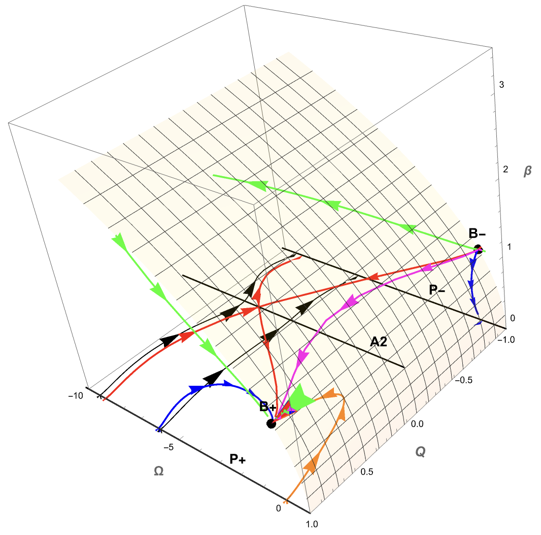
Figure 1: Phase portrait of the invariant submanifold $\zeta=0$ for $\omega=0$. Some trajectories starting from the matter dominated critical line $P_{+}$ as $\tau\rightarrow-\infty$ converge to the dark energy dominated point $B_{+}$ as $\tau\rightarrow\infty$, while others after some expansion begin contracting and collapse to a big crunch at $P_{-}$. Some trajectories which are past asymptotic to $B_{-}$ evolve to the future attractor $B_{+}$, while others evolve to $P_{-}$.

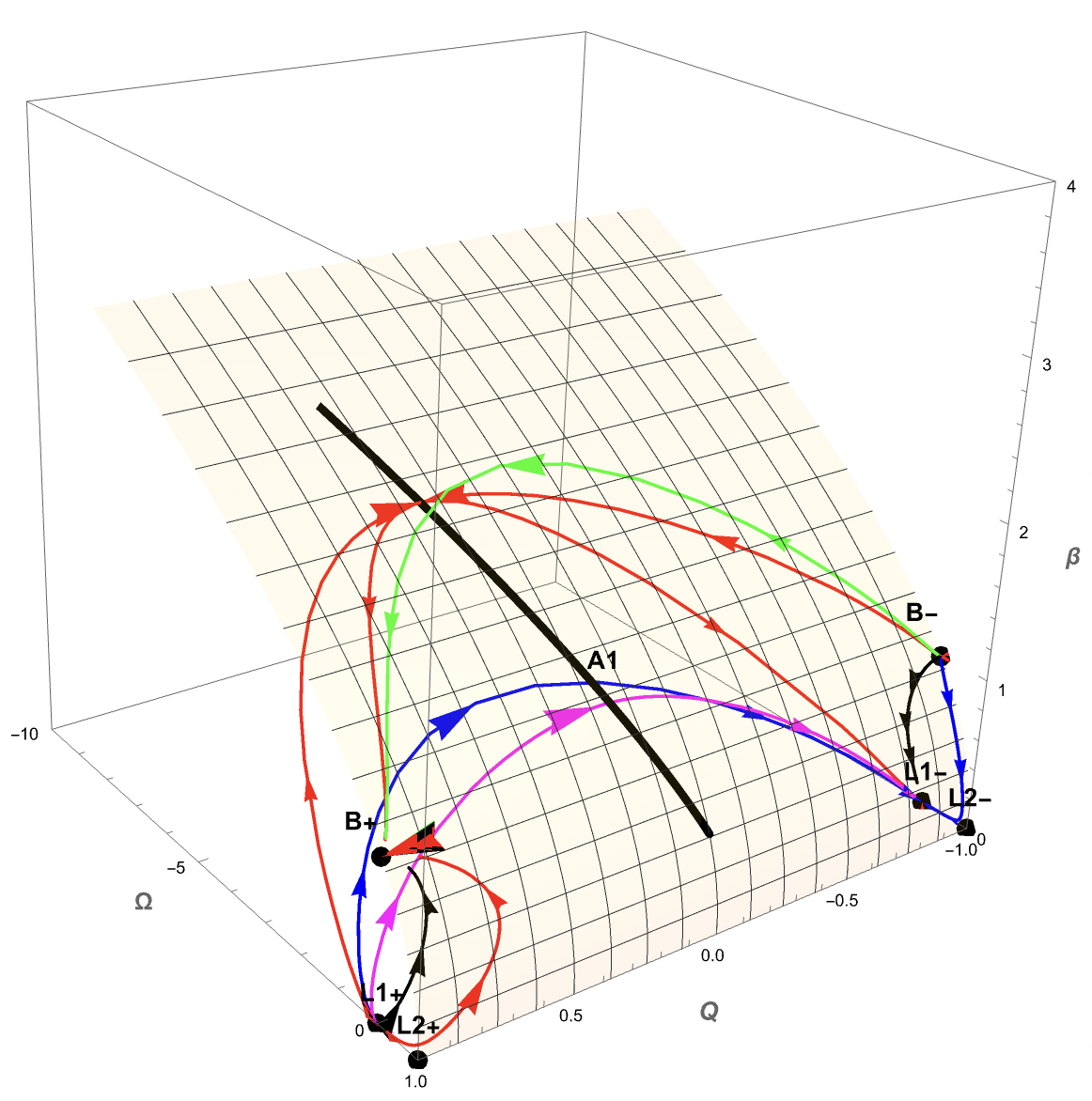
Figure 2: Phase portrait of the invariant submanifold $\zeta=0$ for $\omega=1/3$. Some trajectories starting from the ordinary matter dominated critical line $L_{1+}$ and from the dark matter dominated critical line $L_{2+}$ as $\tau\rightarrow-\infty$ converge to the dark energy dominated point $B_{+}$ as $\tau\rightarrow\infty$, while others after some expansion begin contracting and collapse to a big crunch at $P_{-}$. Some trajectories which are past asymptotic to $B_{-}$ evolve to the future attractor $B_{+}$, while others evolve to $L_{1-}$ or $L_{2-}$.

The behaviour of the variable $\zeta$ for some points close to the submanifold depends almost exclusively on the potential. By explicitly analyzing the behaviour of $\zeta$ as a function of $t$, one can gain insights into the curves and expect a relationship between the behaviours with cosmological time and transformed time. However, for more precision, it is advisable to examine the dynamics around the points belonging to the submanifold, either using the eigenvalues of the variation matrix, if applicable, or the center manifold, if necessary. Lastly, it will depend on the potential if the submanifold is reachable from outside.

3.2.2 Submanifold $\beta=0$

The critical points and their corresponding dynamics in the submanifold are illustrated in Fig. 3:

• For $\omega=0$ : $P_{+}$ exhibits repulsive behaviour in the noncritical axes, while $P_{-}$ displays attractive behaviour in the noncritical axes.

• For $\omega=1/3$ : $L_{1+}$ exhibits repulsive behaviour, $L_{1-}$ has attractive behaviour, and both $L_{2+}$ and $L_{2-}$ behave as saddles

Note that for $\beta=0$, the equation for $\zeta$ vanishes (assuming that $\zeta^{2}(\mu(\zeta)-3/2)$ does not diverge for the conditions in which $\beta$ vanishes), also the contribution of $\zeta$ to the remaining system is null; therefore, it is enough to graph the coordinates $(Q,\tilde{\Omega}_{\lambda})$. In Fig. 3 we plot the phase portrait of the invariant submanifold $\beta=0$ for $\omega=0$ and $\omega=1/3$. The trajectories observed are past asymptotic to a matter dominated critical line which after some expansion enter the contracting phase space and collapse to a big crunch.

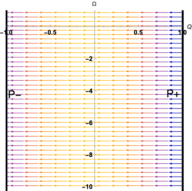
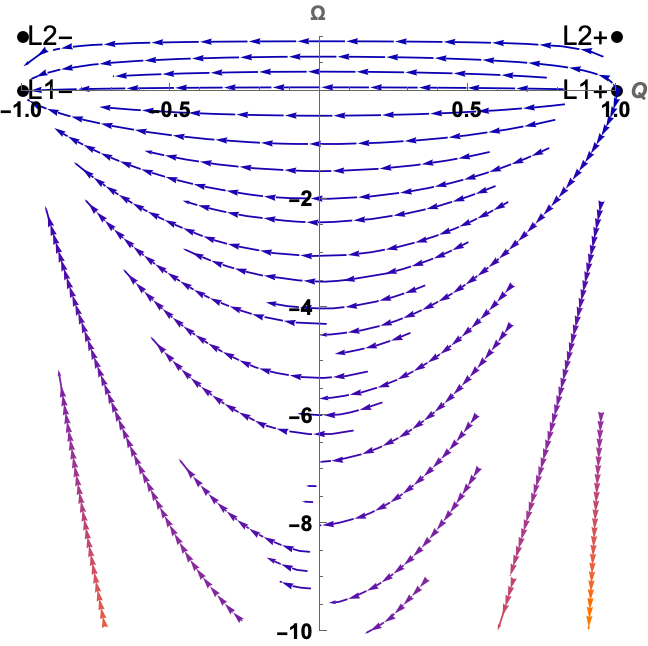
Figure 3: Phase portraits of the invariant submanifold $\beta=0$ for $\omega=0$ (left panel) and $\omega=1/3$ (right panel). Trajectories starting from the matter dominated line $P_{+}$ as $\tau\rightarrow-\infty$ end at $P_{-}$ as $\tau\rightarrow\infty$. Analogously, trajectories starting from the ordinary matter dominated line $L_{1+}$ or from the dark matter dominated line $L_{2+}$ end at $L_{1-}$ or $L_{2-}$.

The analysis of the behaviour on the $\beta$ axis, which is important to determine if a trajectory stays in the neighborhood of the submanifold, is difficult due to the dependence of $\beta$ on $V$ and $D$. It is possible to obtain this information by analyzing the behaviour in the neighborhood of the critical points belonging to the submanifold. For instance, for $P_{-}$ the behaviour is attractive, while for $P_{+}$ it is repulsive along this axis. Again, regarding whether the submanifold can be accessed from an external point depends on the potential.

3.3 Specific potentials

In this section we explore the dynamics of the system for two specific potentials of the mimetic field: the inverse square potential and the exponential potential.

3.3.1 Inverse square potential

Here, we consider the potential $V(\phi)=\gamma/\phi^{2}$, where $\gamma$ is a coupling constant. In this case we find that $\mu(\zeta)=3/2$ and $\zeta=\frac{2}{\kappa\gamma^{1/2}}$ become constants; therefore, the dynamical system reduces to a three-dimensional autonomous dynamical system given by Eqs. (3.4)-(3.6) with $\zeta$ constant.

The critical points of the system are shown in Table 3 and the eigenvalues of the Jacobian matrix which characterize their dynamical behaviour are shown in Table 4. Note that the Einstein static solutions $A_{1}$ and $A_{2}$ disappear for this potential, and also the solutions $B_{+}$ and $B_{-}$.

Table 3: Fixed points of the dynamical system (3.4)-(3.7) and some physical quantities for the inverse square potential. In the formulas below $\zeta=\frac{2}{\kappa\gamma^{1/2}}$.

Label	$\tilde{\Omega}_{\lambda}$	$\beta$	$Q$	Existence	$\Omega_{\rho}$	$\Omega_{\lambda}$	$\Omega_{\phi}$	$\Omega_{k}$	$q$
$C_{1+}$	$-\frac{3(1+\omega)^{3}}{\omega\zeta^{2}}$	$\frac{(1+\omega)\sqrt{3}}{\zeta}$	1	$\omega\neq 0$, $\zeta>0$	$\frac{3+\omega(\zeta^{2}+6+3\omega)}{\zeta^{2}\omega}$	$-\frac{3(1+\omega)^{3}}{\omega\zeta^{2}}$	$\frac{3(1+\omega)^{2}}{\zeta^{2}}$	0	$\frac{1}{2}(1+3\omega)$
$C_{1-}$	$-\frac{3(1+\omega)^{3}}{\omega\zeta^{2}}$	$-\frac{(1+\omega)\sqrt{3}}{\zeta}$	-1	$\omega\neq 0$, $\zeta<0$	$\frac{3+\omega(\zeta^{2}+6+3\omega)}{\zeta^{2}\omega}$	$-\frac{3(1+\omega)^{3}}{\omega\zeta^{2}}$	$\frac{3(1+\omega)^{2}}{\zeta^{2}}$	0	$\frac{1}{2}(1+3\omega)$
$C_{2+}$	$\frac{1}{6}\zeta(\sqrt{12+\zeta^{2}}-\zeta)$	$\frac{\sqrt{12+\zeta^{2}}-\zeta}{2\sqrt{3}}$	1		0	$\frac{1}{6}\zeta(\sqrt{12+\zeta^{2}}-\zeta)$	$\frac{1}{12}(\sqrt{\zeta^{2}+12}-\zeta)^{2}$	0	$\frac{1}{4}\zeta(\sqrt{\zeta^{2}+12}-\zeta)-1$
$C_{2-}$	$-\frac{1}{6}\zeta(\sqrt{12+\zeta^{2}}+\zeta)$	$\frac{\sqrt{12+\zeta^{2}}+\zeta}{2\sqrt{3}}$	-1		0	$-\frac{1}{6}\zeta(\sqrt{12+\zeta^{2}}+\zeta)$	$\frac{1}{12}(\sqrt{\zeta^{2}+12}+\zeta)^{2}$	0	$-\frac{1}{4}\zeta(\sqrt{\zeta^{2}+12}+\zeta)-1$
$D$	$\frac{2}{3}$	$\frac{1}{\sqrt{3}}$	$\frac{\zeta}{2}$	$\zeta\neq 0$, $Q\neq\pm 1$	0	$\frac{8}{3\zeta^{2}}$	$\frac{4}{3\zeta^{2}}$	$1-\frac{4}{\zeta^{2}}$	0
$L_{1+}$	0	0	1		1	0	0	0	$\frac{1}{2}(1+3\omega)$
$L_{2+}$	1	0	1		0	1	0	0	$\frac{1}{2}$
$L_{1-}$	0	0	-1		1	0	0	0	$\frac{1}{2}(1+3\omega)$
$L_{2-}$	1	0	-1		0	1	0	0	$\frac{1}{2}$
$P_{+}$	$\tilde{\Omega}_{\lambda}\leq 1$	0	1	$\omega=0$	$1-\Omega_{\lambda}$	$\Omega_{\lambda}\leq 1$	0	0	$\frac{1}{2}$
$P_{-}$	$\tilde{\Omega}_{\lambda}\leq 1$	0	-1	$\omega=0$	$1-\Omega_{\lambda}$	$\Omega_{\lambda}\leq 1$	0	0	$\frac{1}{2}$

Table 4: Eigenvalues and stability of fixed points of the dynamical system (3.4)-(3.7) for the inverse square potential. In the formulas below we have defined $\xi_{\pm}(\zeta)=\zeta^{2}\pm\zeta\sqrt{\zeta^{2}+12}+12\omega$.

Label	$\lambda_{1}$	$\lambda_{2}$	$\lambda_{3}$	Dynamical Character
$C_{1+}$	$-\frac{3\left((1-\omega)\zeta+\sqrt{24(1+\omega)^{3}+(1+3\omega)^{2}\zeta^{2}}\right)}{4\zeta}$	$-\frac{3\left((1-\omega)\zeta-\sqrt{24(1+\omega)^{3}+(1+3\omega)^{2}\zeta^{2}}\right)}{4\zeta}$	$1+3\omega$	saddle
$C_{1-}$	$\frac{3\left((1-\omega)\zeta+\sqrt{24(1+\omega)^{3}+(1+3\omega)^{2}\zeta^{2}}\right)}{4\zeta}$	$\frac{3\left((1-\omega)\zeta-\sqrt{24(1+\omega)^{3}+(1+3\omega)^{2}\zeta^{2}}\right)}{4\zeta}$	$-(1+3\omega)$	saddle
$C_{2+}$	-$\frac{3}{8}\left(\xi_{-}(\zeta)+8(1-\omega)+\frac{1}{3}|\xi_{-}(\zeta)|\right)$	-$\frac{3}{8}\left(\xi_{-}(\zeta)+8(1-\omega)-\frac{1}{3}|\xi_{-}(\zeta)|\right)$	$-2+\frac{1}{2}\zeta(-\zeta+\sqrt{\zeta^{2}+12})$
$C_{2-}$	$\frac{3}{8}\left(\xi_{+}(\zeta)+8(1-\omega)-\frac{1}{3}|\xi_{+}(\zeta_{*})|\right)$	$\frac{3}{8}\left(\xi_{+}(\zeta)+8(1-\omega)+\frac{1}{3}|\xi_{+}(\zeta)|\right)$	$2+\frac{1}{2}\zeta(\zeta+\sqrt{\zeta^{2}+12})$
$D$	$1-\frac{\zeta}{2}$	$-1-\frac{\zeta}{2}$	$-\frac{1}{2}\zeta(1+3\omega)$	saddle for $-2<\zeta<2$
$L_{1+}$	$3\omega$	$\frac{3(1+\omega)}{2}$	$1+3\omega$	unstable
$L_{2+}$	1	$-3\omega$	$\frac{3}{2}$	unstable for $\omega=0$, saddle for $\omega\neq 0$
$L_{1-}$	$-3\omega$	$-\frac{3}{2}(1+\omega)$	$-(1+3\omega)$
$L_{2-}$	-1	$3\omega$	$-\frac{3}{2}$	saddle for $\omega\neq 0$
$P_{+}$	0	$\frac{3}{2}$	1	unstable
$P_{-}$	0	$-\frac{3}{2}$	-1

To understand the global nature of the model, it is necessary essentially to make a conformal compactification of the entire phase space of the solutions. The critical points at infinity can be identified by projecting onto the Poincaré sphere, as outlined in appendix C.

Now, it is convenient to write the dynamical equations as

$$\tilde{\Omega}_{\lambda}^{\prime}=\hat{P}(\tilde{\Omega}_{\lambda},\beta,Q)\,,\,\,\,\,\,\beta^{\prime}=\hat{Q}(\tilde{\Omega}_{\lambda},\beta,Q)\,,\,\,\,\,Q^{\prime}=\hat{R}(\tilde{\Omega}_{\lambda},\beta,Q)\,,$$ (3.8)

where $\hat{P}$, $\hat{Q}$ and $\hat{R}$ are polynomial functions of the dynamical variables. Since $Q$ is compact, it is enough to project only the variables $\tilde{\Omega}_{\lambda}$ and $\beta$ on the Poincaré sphere. Therefore, we define the following coordinates on the Poincaré sphere

$$X=\frac{\tilde{\Omega}_{\lambda}}{\sqrt{1+\tilde{\Omega}_{\lambda}^{2}+\beta^{2}}}\,,\,\,\,\,Y=\frac{\beta}{\sqrt{1+\tilde{\Omega}_{\lambda}^{2}+\beta^{2}}}\,,\,\,\,\,Z=\frac{1}{\sqrt{1+\tilde{\Omega}_{\lambda}^{2}+\beta^{2}}}\,.$$ (3.9)

So, at infinity ($Z\rightarrow 0$) the dynamical system has the form

$$X^{\prime} = -Y(X\hat{Q}^{*}-Y\hat{P}^{*})\,,$$

$$Y^{\prime} = X(X\hat{Q}^{*}-Y\hat{P}^{*})\,,$$

$$Q^{\prime} = \hat{R}^{*}\,,$$ (3.10)

where the polynomials $\hat{P}^{*}$, $\hat{Q}^{*}$ and $\hat{R}^{*}$ are given by

$$\hat{P}^{*} = \sqrt{3}zY^{3}-3(1+\omega)QXY^{2}\,,$$

$$\hat{Q}^{*} = -\frac{3}{2}(1+\omega)QY^{3}\,,$$

$$\hat{R}^{*} = \frac{3}{2}(1+\omega)(1-Q^{2})Y^{2}\,.$$ (3.11)

Therefore, the critical points/lines $(X,Y,Q)$ at infinity are

$P_{1}$: $(\pm 1,0,Q)$, which corresponds to critical lines

$P_{2}$: $(-\cos\theta,\sin\theta,-1)$ and its antipodal $(\cos\theta,-\sin\theta,-1)$

$P_{3}$: $(\cos\theta,\sin\theta,1)$ and its antipodal $(-\cos\theta,-\sin\theta,1)$

where $\theta=\arctan\left(\frac{\sqrt{3}(1+\omega)}{2\zeta}\right)$. However, it is straightforward to verify that only the critical line $P_{1}$: $(-1,0,Q)$ is located within the physical space $\tilde{\Omega}_{\lambda}\leq 1-\beta^{2}$. Nevertheless, the analysis of the dynamics near this line is a bit difficult because the compactification can end up canceling the dynamics of components that are not at infinity, due to either the compactified variables or the time rescaling. Graphically, however, the variables not projected on the Poincaré sphere show dynamics. This should be interpreted as indicating that the variables with canceled dynamics will undergo a slower evolution than those without. Therefore, the equations are analyzed with the aid of graphics to better understand and visualize these dynamics.

In Fig. 4 we plot the global phase portrait of the dynamical system for $\kappa\gamma^{1/2}=4/3$. This figure shows that the phase space is divided into two halves, one corresponding to a contracting epoch ($Q<0$) and the other to an expanding epoch ($Q>0$). The dynamical system is bounded by the $Y=0$ ($\beta=0$), $Q=\pm 1$, and $\tilde{\Omega}_{\rho}=0$ invariant submanifolds. Some trajectories which are past asymptotic to the matter dominated critical line $P_{+}$ with a sufficiently small value of $\Omega_{\phi}$ after some expansion enter the contracting phase space and collapse to a big crunch at $P_{-}$. Conversely, models starting from $P_{+}$ with a large enough value of $\Omega_{\phi}$ evolve to the future attractor $C_{2+}$, which represents a solution dominated by dark matter and dark energy, exhibiting acceleration for $\zeta<2$ (Table 3). Also, there are trajectories past asymptotic to $C_{2-}$ that evolve to $C_{2+}$. Other trajectories past asymptotic to $C_{2-}$ enter the contracting phase space and recollapse to a big crunch at $P_{-}$. Additionally, we observe trajectories that approximate to the uniformly expanding solution, point $D$ with coordinates $X=1/2$, $Y=\sqrt{3}/4$, $Q=\zeta/2$, and then collapse to a big crunch. Notice that points $C_{2+}$, $C_{2-}$ and $D$ lie on the $\rho=0$ boundary. On this boundary, there exists a trajectory, among others, that is past asymptotic to point $C_{2-}$ and evolves to $D$.

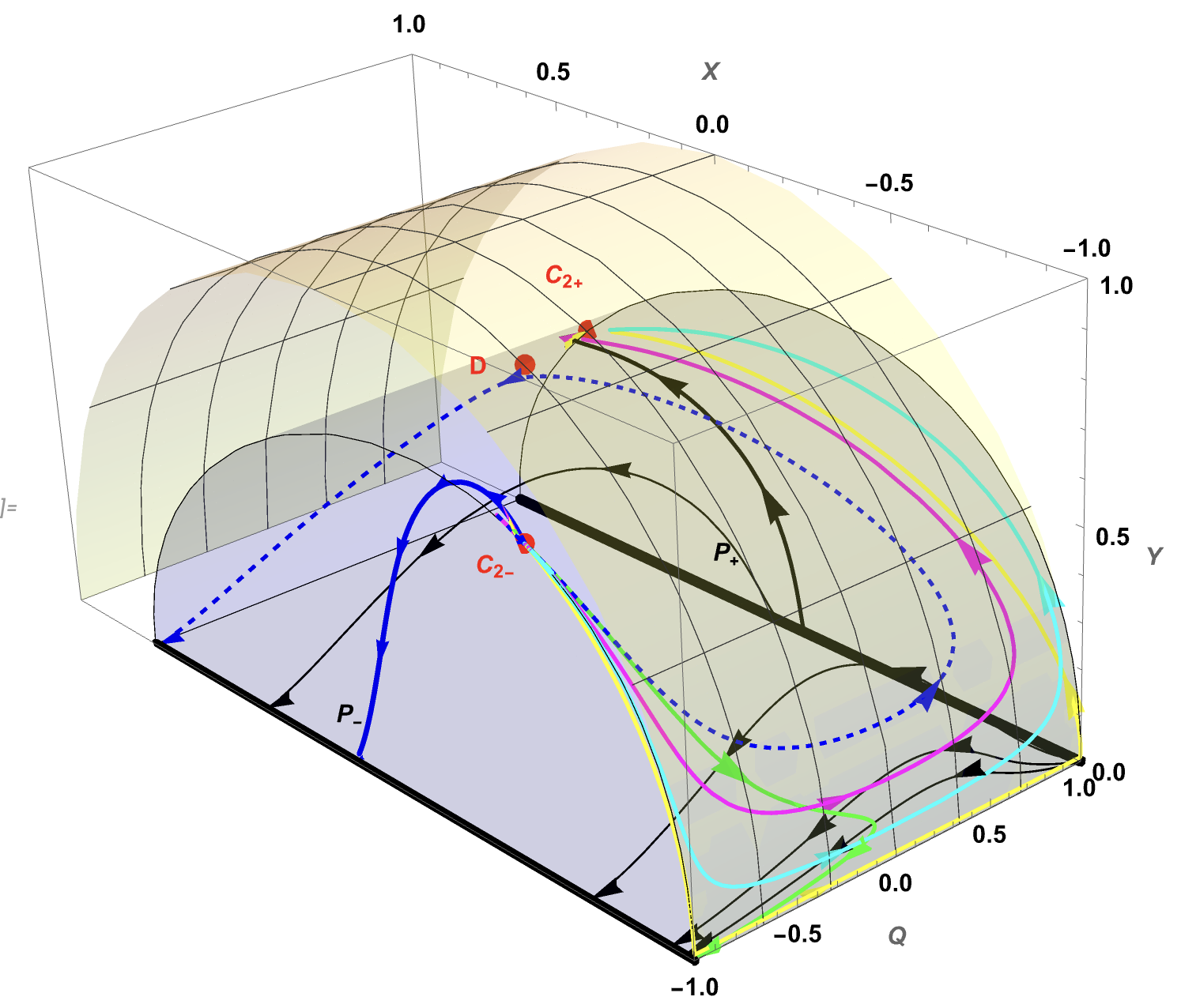
Figure 4: Global phase portrait for the inverse square potential with $\zeta=3/2$. The solutions of the system are $C_{2+}$, $C_{2-}$, $D$, $P_{+}$, $P_{-}$ and the points $X=-1$, $Y=0$, $Q=\pm 1$. Some trajectories starting from the matter dominated critical line $P_{+}$ converge asymptotically to $C_{2+}$ which represents a solution dominated by dark matter and dark energy. We also observe trajectories starting from the contracting solution $C_{2-}$ which converge to the point $C_{2+}$. In addition, some trajectories after some expansion begin contracting and collapse to a big crunch at $P_{-}$.

To analyze the variations, it is convenient to perform the projection described in the appendix D, given that $Q$ varies slowly in relation to $\Omega_{\lambda}$ and $\beta$, and $\zeta$ remains constant. The following change of variable is considered

$$\xi=-\frac{Y}{X}\,,\,\,\,\,\,\chi=-\frac{Z}{X}\,.$$ (3.12)

For these variables and $\omega=0$ the system of equations is the following:

$$Q^{\prime}=\frac{1}{2}(1-Q^{2})(3\xi^{2}-\chi^{2})\,,\,\,\,\,\,\xi^{\prime}=\frac{1}{2}\xi\left(3Q(\chi^{2}+\xi^{2})+\sqrt{3}\zeta\xi(2\xi^{2}-\chi)\right)\,,\,\,\,\,\,\chi^{\prime}=\chi\xi^{2}\left(3Q+\sqrt{3}\zeta\xi\right)\,,$$ (3.13)

and the variation matrix for the line $(-1,0,Q)$ is null; therefore, its eigenvalues are null, and correspond to a degenerate line which will be analyzed according to the method exposed in appendix E. Now, note that the solution is independent of $Q$ so it should not show dynamics in the neighborhood (remember that in this context it means that it varies more slowly than the other variables), so we could consider it as a constant, just like $\zeta$ for the potential is constant. Using the angular equation in the neighborhood of interest, it is possible to see that the solutions are $\theta=0,\pi/2$, and additionally, for $\frac{\zeta}{Q}<0$, the solution is $\theta=\frac{1}{2}\text{arccot}\left(-\frac{\zeta}{2\sqrt{3}Q}\right)$. So, reviewing the radial equation in the neighborhood, it is possible evaluate the behaviour (if the radial component is also canceled, the analysis must be discarded as insufficient). Therefore, for the last solution it can be said that it is:

• repulsive for $Q>0$ and $\zeta<0$

• attractive for $Q<0$ and $\zeta>0$

the $\theta=0$ solution is

• repulsive for $Q>0$

• attractive for $Q<0$

and the $\theta=\pi/2$ solution does not exhibit radial dynamics. At this order the radial behaviour is annulled, so higher orders terms must be considered; however, graphically it can be seen that the evolution is angular and not radial, so it is discarded.

As previously mentioned, it is still necessary to assess the dynamics of the variable $Q$ and does not disregard it.
Then, it is easy to see that for large $\beta$, $Q^{\prime}>0$. Thus, the system will exhibit saddle behaviour with the critical point at $(Q,X,Y)=(\pm 1,-1,0)$. However, it is important to note that the possibility of a small and constant $\beta$ is also contained within this critical point. In particular, for $\beta<\frac{1}{\sqrt{3}}$ and under certain circumstances, such as $\zeta>0$ and $Q<0$, $Q^{\prime}<0$ will occur, causing $(Q,X,Y)=(-1,-1,0)$ to act as an attractor, while the point $(Q,X,Y)=(1,-1,0)$ in this example would require even more specific conditions and could act as a repulsor. The necessary conditions for the attractor and repulsor behaviour will not be further explored, but it can be shown from a simple analysis of the equations. It suffices to conclude that the system truly exhibits critical behaviour at the points $(Q,X,Y)=(\pm 1,-1,0)$ and can exhibit saddle behavior or attractor and repulsor behaviour, respectively, for the points $Q=-1$ and $Q=1$, depending on the initial conditions of the solution. The behaviour of attractor and repulsor is not immediately visible, but it can be better understood by observing the graphics where the saddle behaviour is not manifested for a certain space. Analytically, it can also be seen for a constant $\beta$; however, this solution is overshadowed by the behaviour of $Y=0$, which also includes solutions where $\beta$ grows slower than $\tilde{\Omega}_{\lambda}$. As mentioned before, the graphics provide a clearer understanding.

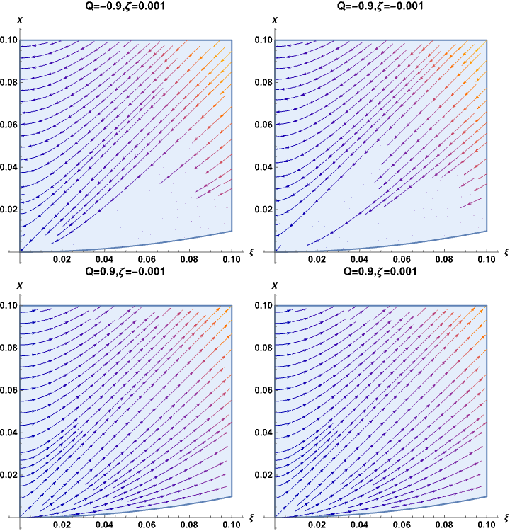
Figure 5: Plane $(\xi,\chi)$. Depending on the sign of $Q$, the behaviour of the point will be either repulsive or attractive in the plane. The sign of $\zeta$ determines whether there will be one or two directions associated with the same behaviour.

Then, the attractor-repulsor behaviour or the saddle behaviour depends exclusively on the sign of $Q^{\prime}$ and the initial value of $\beta$.

Equivalently, for $\omega=1/3$ , the equations are:

$$Q^{\prime} = \frac{1}{2}(1-Q^{2})(4\xi^{2}-2\chi^{2}-\chi)\,,$$

$$\xi^{\prime} = \frac{1}{2}\xi\left(Q(4\xi^{2}+2\chi^{2}-\chi)+\sqrt{3}\zeta\xi(2\xi^{2}-\chi)\right)\,,$$

$$\chi^{\prime} = \sqrt{3}\zeta\xi^{3}\chi-Q\chi(\chi+\chi^{2}-4\xi^{2})\,.$$ (3.14)

The variation matrix for the analyzed point have null eigenvalues, so its structure is evaluated using polar coordinates (see appendix E). From this the conclusions are slightly more difficult to analyze analytically. Firstly, in the plane $(\xi,\chi)$ the angles $\theta=0,\pi/2$ are obtained, then its dynamics will be the following:

1. For $\theta=0$, the solution is

• attractive for $Q>0$

• repulsive for $Q<0$

2. For $\theta=\pi/2$, the solution is

• repulsive for $Q>0$

• attractive for $Q<0$

Then, it is necessary to note that the sign of $Q^{\prime}$ will be described such that $sign(Q^{\prime})=sign(4\xi^{2}-2\chi^{2}-\chi)$. This expression also seems to divide the regions of influence of behaviours, which by analyzing the graphics, seem to be mostly disconnected. In Figs. 5 and 6 we show some example graphics.

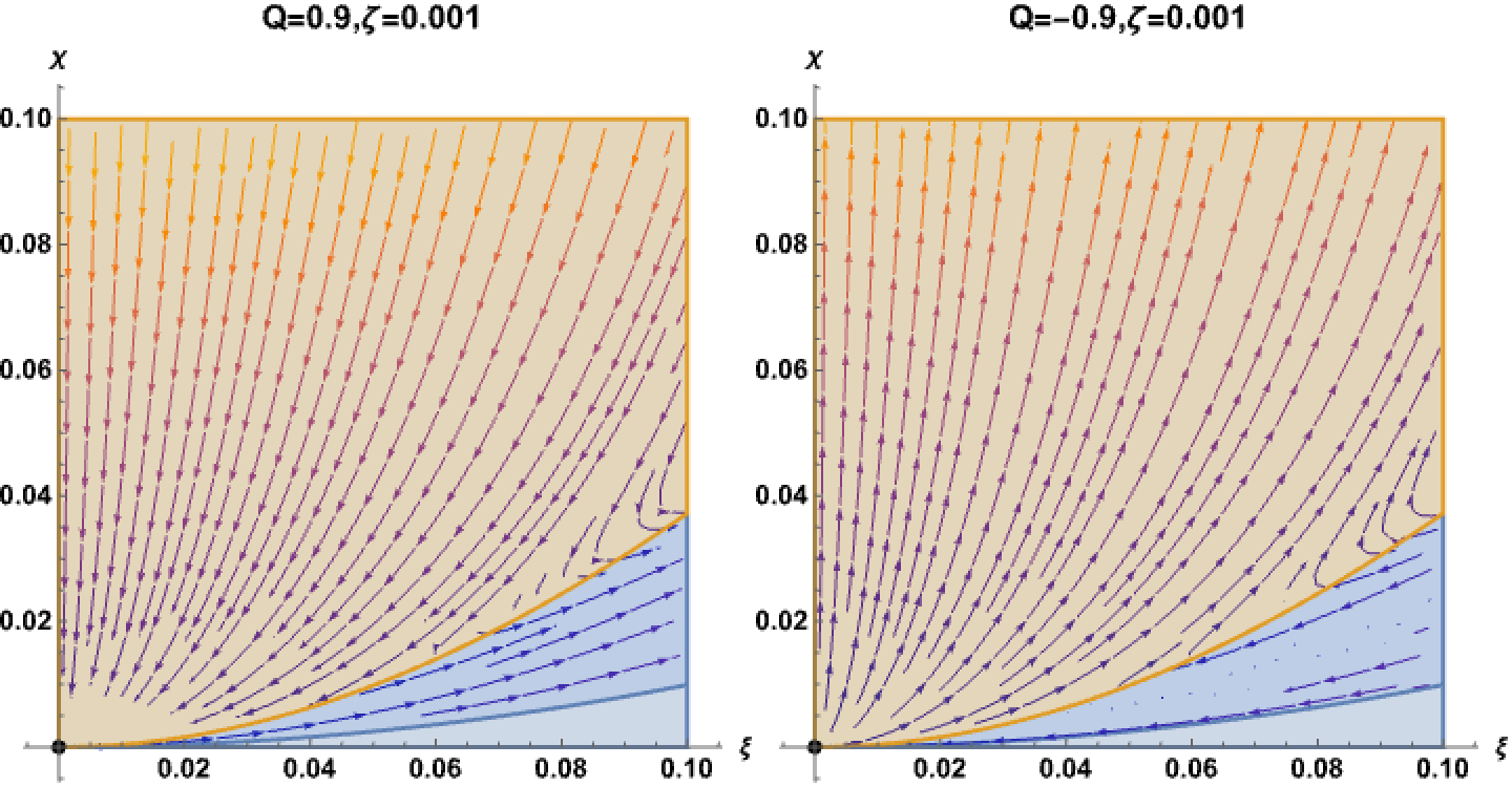
Figure 6: Plane $(\xi,\chi)$. In this plane, the behaviour will be repulsive or attractive depending on the sign of $Q$ and the sign of $4\xi^{2}-2\chi^{2}-\chi$ (blue for positive and red for negative) .

From the figure, it can be asserted that the points act as saddles, with $Q=\pm 1$ representing the real critical points. based on this observation, it is possible to say that there will be two main trajectories, both interacting with the saddle points but in different directions. Additionally, there might be a third type of trajectory that undergoes a change in direction. It is unlikely that trajectories leading to attractor-repulsive points will emerge, and the analysis conducted so far lacks the capability to demonstrate or visualize such occurrences.

3.3.2 Exponential potential

Now, we consider the potential $V(\phi)=V_{0}e^{-\alpha\phi}$. For this potential we find $\mu(\zeta)-3/2=-1/2$ ; therefore, the points $C_{1+}$, $C_{1-}$, $C_{2+}$, $C_{2-}$ and $D$ listed in Table 1 do not manifest in the phase space for this model. All the remaining points/lines correspond to non-accelerating solutions, with the exception of point $B_{+}$ representing a saddle de Sitter point dominated by the mimetic field. This point exhibits unstable behaviour in the $\zeta$ direction. Point $B_{-}$ is the contracting analogue of $B_{+}$. However, it is worth noticing that the invariant submanifold $\zeta=0$ divides the phase space into two regions, preventing trajectories from crossing between them. From Eq. (3.7), we deduce that if $\mu(\zeta)-3/2<0$ as $\zeta\rightarrow 0$, then $\zeta^{\prime}>0$ and point $B_{+}$ acts as a future attractor for trajectories in the region $\zeta<0$.

On the other hand, no attempt will be made to make graphics that describe the solutions in 4-dimensional space, since regardless of the method for this, it might not be visual enough to be interpreted. However, it is possible to have some degree of understanding by analyzing the invariant submanifolds, and extrapolating the behaviour to their neighborhoods. That being said, the $\zeta=0$ and $\beta=0$ manifolds have a general qualitative behaviour independent of the shape of the potential, so their behaviours are similar to that described in subsection 3.2, added to the analysis of the $\tilde{\Omega}_{\rho}=0$ submanifold, which is now possible to analyze since the potential is known. For this potential, the variable $\zeta$ is given by $\zeta=\frac{\alpha}{\kappa\sqrt{V}}$, with $V=V_{0}e^{-\alpha t}$. Therefore, $\alpha<0$ implies $\zeta<0$, and $\zeta\rightarrow 0$ when $t\rightarrow\infty$. On the other hand, $\alpha>0$ implies $\zeta>0$, and $\zeta\rightarrow\infty$ when $t\rightarrow\infty$, being necessary to consider the critical points at infinity.

Then, the critical points and their respective dynamics in the manifold are detailed in Figs. 7 and 8:

• For both values of $\omega$: $B_{+}$ exhibits saddle behaviour for centre manifold, with $\zeta>0$ representing the unstable direction, and $B_{-}$ shows saddle behaviour for centre manifold, with $\zeta<0$ as the stable direction. However, as previously mentioned, the point $B_{+}$ behaves as an attractor for trajectories in the region $\zeta<0$, while manifesting saddle behaviour for trajectories in the region $\zeta>0$, and only the $\zeta$ direction is unstable.

• For $\omega=0$: $A_{2}$ displays saddle behaviour, but $A_{2}$ is a line where one of its ends touches the submanifold, since we are interested in the neighborhood it must be considered, so, the influence on the subsystem is minimal, $P_{+}$ shows repulsive behaviour in directions other than the critical axis, while $P_{-}$ is the contracting analogue of $P_{+}$

  

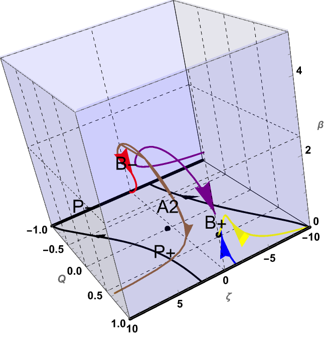
  Figure 7: Phase portrait of the invariant submanifold $\tilde{\Omega}_{\rho}=0$ for $\omega=0$. Some trajectories in the region $\zeta<0$ starting from the matter dominated critical line $P_{+}$ as $\tau\rightarrow-\infty$ converge to the dark energy dominated point $B_{+}$ as $\tau\rightarrow\infty$. In the region $\zeta>0$ we observe trajectories that evolve to some critical point at $\zeta\rightarrow\infty$. Also, there are trajectories which are past asymptotic to $P_{+}$ and collapse to a big crunch at $P_{-}$.

• For $\omega=1/3$: $L_{2+}$ exhibits repulsive behaviour in directions other than the critical axis, $L_{2-}$ exhibits attractive behaviour in directions other than the critical axis and $A_{1}$ shows saddle behaviour. It is important to note that $A_{1}$ is a curve where one of its ends touches the submanifold, as we are interested in the neighborhood it must be considered, so, the influence on the subsystem is minimal

  

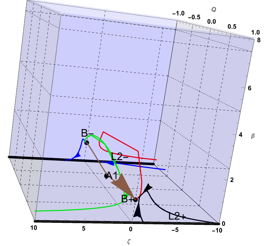
  Figure 8: Phase portrait of the invariant submanifold $\tilde{\Omega}_{\rho}=0$ for $\omega=1/3$. Some trajectories in the region $\zeta<0$ starting from the dark matter dominated critical line $L_{2+}$ as $\tau\rightarrow-\infty$ converge to the dark energy dominated point $B_{+}$ as $\tau\rightarrow\infty$. In the region $\zeta>0$ we observe trajectories that evolve to some critical point at $\zeta\rightarrow\infty$.

The stability in the $\tilde{\Omega}_{\rho}$ axis does not obey a unique behaviour throughout the submanifold and since this term depends on $\rho$ and $D$, the analysis is not easy. On the other hand, it is evident that the submanifold is inaccessible from an external point since $\rho$ must be null for this, so it is only possible if $\rho$ is null by default.

The critical points at infinity can be found by projecting the variables $\tilde{\Omega}_{\lambda},\beta,\zeta$ on the Poincaré sphere, see appendix C. In this case the procedure applied above is generalizable. Here, the equations have the particularity that $\mu(\zeta)=1$, and the coordinates on the Poincaré sphere are given by

$$X = \frac{\tilde{\Omega}_{\lambda}}{\sqrt{1+\tilde{\Omega}_{\lambda}^{2}+\beta^{2}+\zeta^{2}}}\,,\,\,\,Y=\frac{\beta}{\sqrt{1+\tilde{\Omega}_{\lambda}^{2}+\beta^{2}+\zeta^{2}}}\,,$$

$$Z = \frac{\zeta}{\sqrt{1+\tilde{\Omega}_{\lambda}^{2}+\beta^{2}+\zeta^{2}}}\,,\,\,\,W=\frac{1}{\sqrt{1+\tilde{\Omega}_{\lambda}^{2}+\beta^{2}+\zeta^{2}}}\,.$$ (3.15)

At infinity ($W\rightarrow 0$), the dynamical system transforms to

$$X^{\prime} = \sqrt{3}Y^{3}Z(Y^{2}+Z^{2})\,,$$

$$Y^{\prime} = -\sqrt{3}XY^{4}Z\,,$$

$$Z^{\prime} = -\sqrt{3}XY^{3}Z^{2}\,,$$

$$Q^{\prime} = 0\,,$$ (3.16)

we have omitted showing the form of the functions for each derivative after the projection, for simplicity. In the same way as before, the solution inside of the physical space ($X,Y,Z,Q$) can be described as $P_{4}$ : (X,0,Z,Q), with the condition $X^{2}+Z^{2}=1$.

Once again, it becomes evident that the variable $Q$ will be eliminated in the limit as $W\rightarrow 0$, as it is not included in the set of the projected variables. Despite this, a thorough analysis of the equations will be conducted and supported by graphics for enhanced comprehension. On the other hand, it is easy to notice that the solution is indifferent to the values of $X,Z$ which if it is part of the coordinates in the Poincaré sphere, this implies a lack of dynamics in those directions locally, mainly on $Z$ since $X$ is associated with $\tilde{\Omega}_{\lambda}$ and this must still respond to the limitations of the physical phase space.

Accordingly, to analyze the variations, it is convenient to carry out the projection described in appendix D since Q varies slowly with respect to $\tilde{\Omega}_{\lambda}$ , $\beta$ and $\zeta$. The following change of variables is considered

$$\xi=-\frac{Y}{X}\,,\,\,\,\,\,\chi=-\frac{Z}{X}\,,\,\,\,\,\,\eta=-\frac{W}{X}\,.$$ (3.17)

For these variables with $\omega$ as a free parameter, the system of equations is as follows:

$$Q^{\prime} = \frac{1}{2}(-1+Q^{2})\eta\left(3\eta\omega-3\xi^{2}(1+\omega)+\eta^{2}(1+3\omega)\right)\,,$$

$$\xi^{\prime} = \frac{1}{2}\xi\left(\sqrt{3}\chi\xi(-\eta+2\xi^{2})+3Q\eta(\eta^{2}+\xi^{2}-(\eta+\eta^{2}-\xi^{2})\ \omega)\right)\,,$$

$$\chi^{\prime} = \frac{1}{2}\chi\left(\sqrt{3}\chi\xi(\eta+2\xi^{2})+6Q\eta(-\eta(1+\eta)\omega+\xi^{2}(1+\ \omega))\right)\,,$$

$$\eta^{\prime} = \eta\left(\sqrt{3}\chi\xi^{3}+3Q\eta(-\eta(1+\eta)\omega+\xi^{2}(1+\ \omega))\right)\,.$$ (3.18)

Note that these coordinates were constructed in the same way as in the 2D case, note also that they represent a tangent space to the point $(Q,X,Y,Z)=(Q,-1,0,0)$ given the freedom that exists in $(X,Z)$ and for simplicity those values have been chosen. Then, the variation matrix associated with this system for $(Q,\xi,\chi,\eta)=(Q,0,\chi,0)$ is null, so the method exposed in appendix E can be used. To describe the dynamics, two coordinates will suffice since $\chi$ is not relevant; therefore, polar coordinates are used such that $\xi=r\cos\theta$ and $\eta=r\sin\theta$. Then, for $\omega=0$ the angular equation will have two solutions, $\theta=0,\pi/2$ also note that $0\leq\theta\leq\pi/2$. For $\theta=0$ it will be fulfilled that $r^{\prime}$ will have the same sign as $\chi$, in other words for $\zeta>0$ we have repulsive behaviour and for $\zeta<0$ attractive behaviour. On the other hand, for $\theta=\pi/2$ both components (radial and angular) cancel out and the behaviour is not noticeable graphically. As already said, the analysis of $Q^{\prime}$ must be done with the equation directly. To explain the curves from the analysis is not easy. First, $Q^{\prime}$ will be positive for $\beta>1/\sqrt{3}$ and negative otherwise, then as we have already seen for a potential $V(\phi)=V_{0}e^{-\alpha\phi}$ with $\alpha>0$ by definition $\zeta$ will be positive and therefore infinity will be repulsive, also it is necessary to consider that the point $B_{-}$ will be mainly repulsive except in $\zeta$ and on the contrary $B_{+}$ has the reverse behaviour. Finally, if we have a curve able of maintaining $Q^{\prime}>0$ it will be repelled towards infinity and then returned to the finite region towards $B_{+}$, on the contrary, if we obtain a curve able of maintaining $Q^{\prime}<0$, this curve will not be cast to infinity, so in this case the analysis is irrelevant.

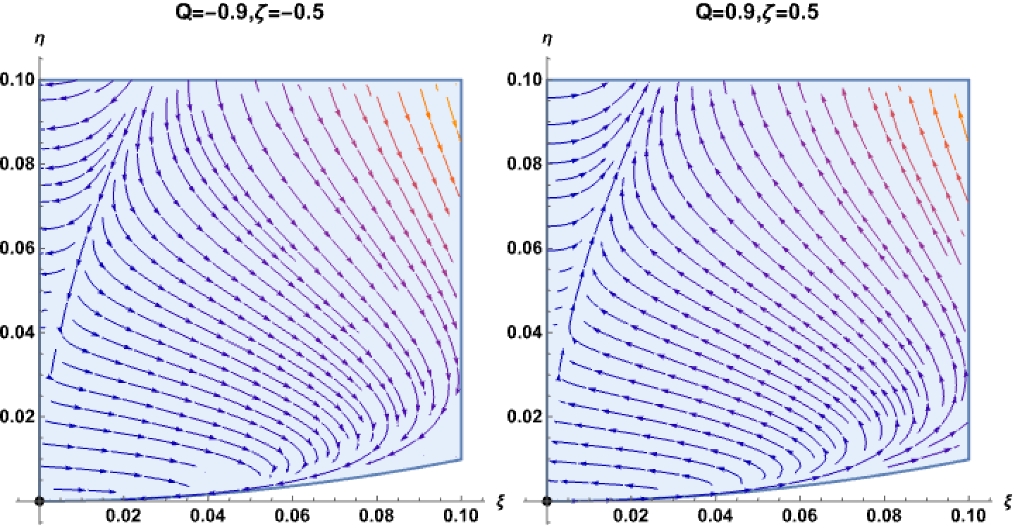
Figure 9: Plane $(\xi,\eta)$. Depending on the sign of $\zeta$, the behaviour of the point will be either repulsive or attractive in the plane.

Then, for $\omega=1/3$ the angular equation will yield three solutions, $\theta=0,\pi/2$, $\theta_{0}$ , with $\tan\theta_{0}=\sqrt{3}\chi/Q$. Given the constraint on $\theta$, the last solution will only exist if $\chi Q>0$. For $\theta=0$ the sign of the radial behaviour will be the same as the sign of $\chi$, similar to $\omega=0$. For $\theta=\pi/2$ the sign of the radial behaviour will be the opposite to the sign of $Q$, and finally, for the solution $\theta_{0}$ to exist, it must exhibit a behaviour opposite to $\chi$. On the other hand, analyzing the behaviour of $Q$ will be more intricate. In the last variables, the sign of $Q^{\prime}$ will be the same as that of $4\xi^{2}-2\eta^{2}-\eta$, and to visualize if there are separated regions with a fixed sign of $Q$, a graphical analysis is employed. In Figs. 9 and 10 we show some example graphics.

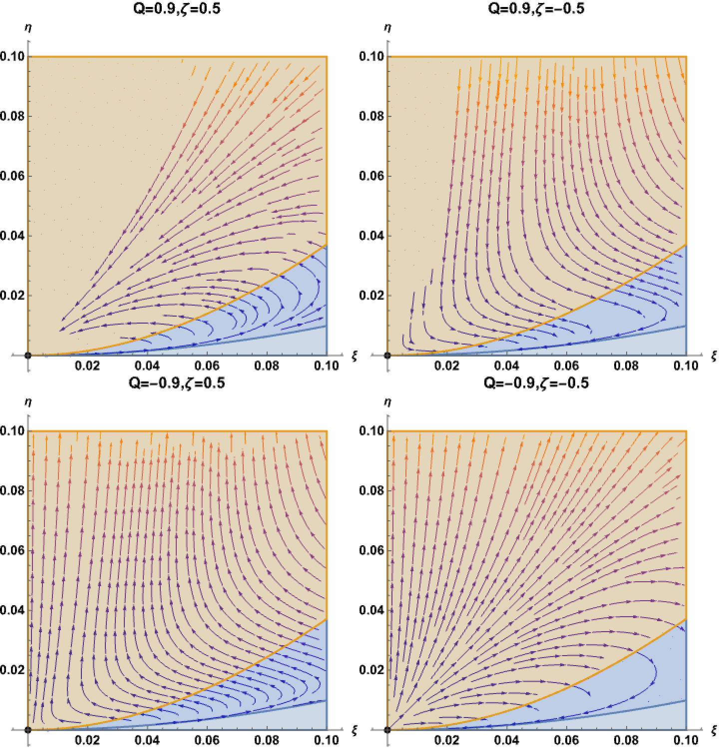
Figure 10: Plane $(\xi,\eta)$. In this plane, the behaviour will be repulsive or attractive depending on the sign of $Q$; furthermore, another invariant trajectory may exist depending on the sign of $Q\zeta$ with the same behaviour, the sign of $Q^{\prime}$ will depend on $4\xi^{2}-2\eta^{2}-\eta$ (blue for positive and red for negative).

Graphically, there seems to be no relationship between the behaviour of $Q$ and the behaviour of ($\xi,\eta$). Having said this, it is not possible to draw a general conclusion. Therefore, each trajectory must be analyzed individually for a comprehensive understanding.

However, in this analysis and under the choice made for the point in the tangent space, the points (Q,X,Y,Z)=(Q,0,0,$\pm$1) have been left out, despite the expectation that the behaviour described in the analysis could be extrapolated to these points. However, it is anticipated that this is not the case and the analysis in question (for both values of $\omega$) must be the following:

It is possible to make a new projection in the tangent space at $Z=1$ (it is enough to analyze only one point since $Z=-1$ is its antipode). To go directly from the original coordinates to the final ones, the following relations are used

$$Q=Q\,,\,\,\,\,\tilde{\Omega}_{\lambda}=\chi/\epsilon\,,\,\,\,\,\beta=\xi/\epsilon\,,\,\,\,\,\zeta=1/\epsilon\,.$$ (3.19)

Rewriting the equations in these new variables with the respective time rescaling (which is evident when explicitly written), it is found that the variation matrix is null, indicating a degenerate point. The procedures detailed in appendix E for slightly degenerated points are applied. Unfortunately, these procedures do not provide detailed insights into the structures around this point; therefore, we proceed to show graphics around these points, where in the new variables they correspond to the points $(Q,\chi,\xi,\epsilon)=(Q,0,0,0)$.

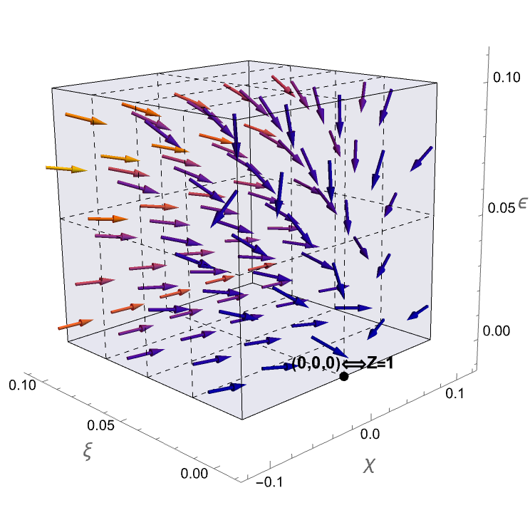
Figure 11: Behaviour around the point $Z=1$ for $\omega=0,1/3$.

In Fig. 11 is possible to see an attractive behavior in all the components, except for $Q$, which requires a separate analysis. Note that the graphic is independent of the values of $\omega$ and $Q$.

It is worth noticing from Eqs. (3.4)-(3.7) with $\omega=0$ that the $\tilde{\Omega}_{\lambda}^{\prime}$ equation decouples. This leads to a three dimensional reduced dynamical system for the variables $Q$, $\zeta$ and $\beta$. So, it is possible to graph the global phase space of this reduced dynamical system. By projecting the coordinates $\zeta$ and $\beta$ on the Poincaré sphere we define

$$X=\frac{\zeta}{\sqrt{1+\beta^{2}+\zeta^{2}}}\,,\,\,\,\,Y=\frac{\beta}{\sqrt{1+\beta^{2}+\zeta^{2}}}\,,\,\,\,\,Z=\frac{1}{\sqrt{1+\beta^{2}+\zeta^{2}}}\,.$$ (3.20)

In Fig. 12 we plot the global phase space of the reduced dynamical system characterized by the coordinates $Q$, $X$ and $Y$ for the exponential potential. The phase space is divided into two halves, one corresponding to a contracting epoch ($Q<0$) and the other representing an expanding epoch ($Q>0$). We can observe that for different values of $X$ some trajectories which are past asymptotic to the matter dominated critical line $P_{+}$, with a sufficiently small value of $\Omega_{\phi}$ after some expansion enter the contracting phase space and collapse to a big crunch at $P_{-}$. On the other hand, in the region $X<0$ ($\zeta<0$), there are models starting from $P_{+}$ with a large enough value of $\Omega_{\phi}$ that evolve to the future attractor $B_{+}$, which represents an expanding de Sitter accelerated solution dominated by the mimetic field. In the region $X>0$ ($\zeta>0$), there are models starting from $P_{+}$ with a large enough value of $\Omega_{\phi}$ that approximate to the point $B_{+}$, then evolve to the point $X=1$, $Y=0$ $Q=1$ (note that $X=1$ coincides with $Z=1$ in the previous analysis) at infinity, and then move to the point $X=1$, $Y=0$, $Q=-1$. Also, in $X>0$, we observe trajectories that are past asymptotic to $B_{-}$ and evolve to the point $X=1$, $Y=0$, $Q=-1$ at infinity. There are trajectories which are past asymptotic as well as future asymptotic to the Einstein static solution $A_{2}$, characterized by coordinates $X=0$, $Y=1/2$, $Q=0$.

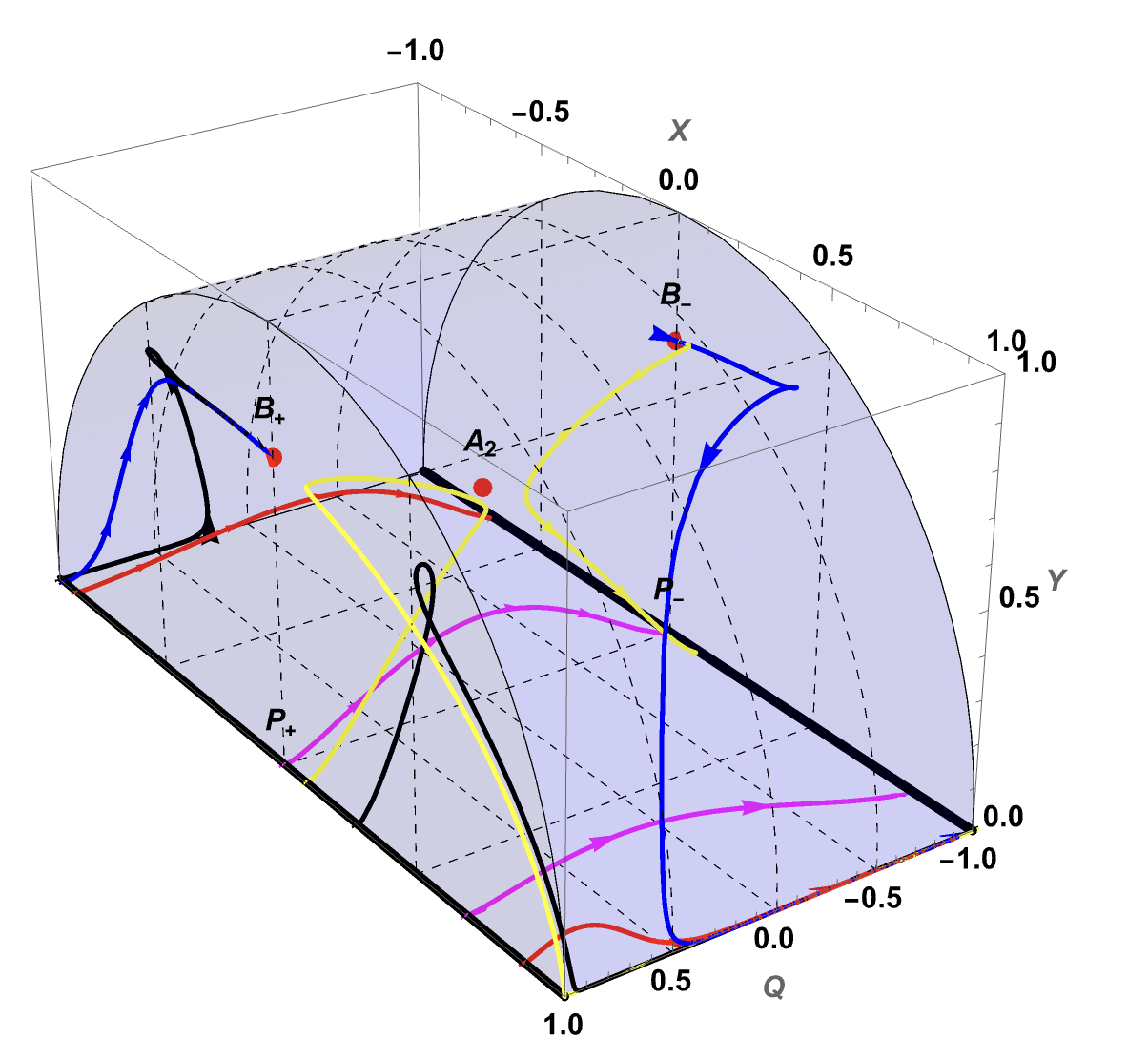
Figure 12: Global phase portrait of the reduced dynamical system for exponential potential with $\omega=0$. The solutions of the system are $B_{+}$, $B_{-}$, $A_{2}$, $P_{+}$, $P_{-}$ and the points $X=1$, $Y=0$, $Q=\pm 1$. Some trajectories in the region $X<0$ ($\zeta<0$) which are past asymptotic to the matter dominated critical line $P_{+}$ evolve to the mimetic field dominated point $B_{+}$. Some trajectories in the region $X>0$ ($\zeta>0$) which are past asymtotic to the matter dominated critical line $P_{+}$ evolve to the critical point at infinity $X=1$, $Y=0$, $Q=1$ and then move to $X=1$, $Y=0$, $Q=-1$. Also, there are trajectories that after some expansion begin contracting and collapse to a big crunch at $P_{-}$.

In this context, it can be demonstrated that in the vicinity of infinity (where $X=1$ in the last defined coordinates), $Q^{\prime}<0$ holds for any $Q$, indicating that only $(Q,X,Y)=(-1,1,0)$ would act as an attractor, while $(Q,X,Y)=(1,1,0)$ would be a saddle point. Special conditions where $Q^{\prime}>0$ can be added, but they are transient. To understand this, it must be taken into account that the form of $Q$ and the temporal rescaling suggest that the submanifolds $Q=\pm 1$ are inaccessible, so we eventually return to the first case. In summary, some curves may experience a transitory asymptotic approach to $(Q,X,Y)=(1,1,0)$ of long duration. However, this may not be numerically appreciable since, as previously mentioned, $Q=1$ is an invariant submanifold, and due to lack of precision, a point in the vicinity might be approached as one of the submanifolds. The next analysis provides a thorough exploration of the behaviour of the system

$$Q^{\prime}=(1-Q^{2})\frac{3\beta^{2}-1}{2}\quad \triangle_{Q}\quad 0$$

$$3\beta^{2}-1\quad \triangle_{Q}\quad 0$$

$$\beta^{2}\quad \triangle_{Q}\quad 1/3$$

Here, $\triangle$ denotes some inequality sign, and $\nabla$ its inversion, and

$$\beta^{\prime}=-\frac{\sqrt{3}}{2}\beta^{2}\zeta-\frac{3}{2}\beta Q(\beta^{2}-1)\quad \triangle_{\beta}\quad 0$$

$$-\beta\zeta-\sqrt{3}Q(\beta^{2}-1)\quad \triangle_{\beta}\quad 0$$

$$\beta\zeta+\sqrt{3}Q(\beta^{2}-1)\quad \nabla_{\beta}\quad 0$$

$$\zeta\quad \nabla_{\beta}\quad-\sqrt{3}Q\frac{\beta^{2}-1}{\beta}$$

• Assuming $\beta$ is finite (in this context, $\beta\ll\zeta$), then $\nabla_{\beta}\rightarrow>$ implies $\triangle_{\beta}\rightarrow<$, which in turn implies $\beta^{\prime}<0$. Therefore, with sufficient time at infinity, $\beta^{2}<1/3\Rightarrow\triangle_{Q}\rightarrow<$, leading to $Q^{\prime}<0$.

• If we consider $\beta$ as a variable at infinity (assuming it is in the vicinity of $(X,Y)=(1,0)$, so in the best-case scenario $\beta\gg 0$ and $\beta\ll\zeta$), then.

  $$\zeta\quad \nabla_{\beta}\quad-\sqrt{3}Q\beta+...$$

  Then, under the assumption of being in the mentioned neighborhood, it must hold that $\nabla_{\beta}\rightarrow>$. Following the same reasoning as in the previous point, this implies $\beta^{\prime}<0$. With sufficient time, $\beta^{2}<1/3$, and consequently, $Q^{\prime}<0$. Note that the second condition may not be very evident, but by contradiction, if it is assumed that $\zeta\propto\beta$, it is straightforward to conclude that $(X,Y)\neq(1,0)$.

• Still, there appears to be one apparent option, and it arises when noticing that the inequality expression to evaluate for $\zeta$ diverges at $\beta=0$. However, if enough time has passed for $Q<0$, then the expression will transform back to $\zeta>-\infty$, thus recovering the previous conclusions. If the assumption about $Q$ is not true, perhaps some point in finite space could be dominating the trajectory; however, the curves seem to indicate the opposite.

This brief analysis does not constitute a formal proof but rather provides arguments to estimate its behavior. Therefore, the possibility that some trajectory asymptotically approaches $Q=1$ should not be ruled out. Unfortunately, numerical evaluation does not yield significantly better results.

4 Mimetic field potential analysis

In this section we obtain numerical solutions for the differential equations and explore the dynamics of the Hubble parameter and the scale factor for different mimetic field potentials. Moreover, we compare these solutions with those of the non-flat $\Lambda$CDM model.

It is useful to write the cosmological equations as function of the redshift $z$ to facilitate the comparison of the models with the observational data. The relationship between redshift and scale factor is given by

$$1+z=\frac{a(t_{0})}{a(t)}\,,$$ (4.1)

where $t_{0}$ refers to the present time which will be set to zero. The derivative with respect to cosmic time of this expression results in

$$\frac{dz}{dt}=-(1+z)H\,.$$ (4.2)

Expressed in terms of the parameter $z$, the second Friedmann equation can be written as

$$\frac{dH}{dz}=\frac{3H}{2(1+z)}-\frac{\kappa^{2}}{2(1+z)H}V(t)-\frac{\Omega_{k}H_{0}^{2}(1+z)}{2H}\,,$$ (4.3)

where $t=t(z)$ and the potential $V(t)$ is parametrically considered as $V(z)$. The function $t(z)$ is determined from the equation

$$\frac{dt}{dz}=-\frac{1}{(1+z)H}$$ (4.4)

with the initial condition $t(0)=0$. Additionally, the first Friedmann equation (2.13) evaluated at the present time yields the following constraint among the density parameters

$$1=\Omega_{\rho,0}+\Omega_{\lambda,0}+\Omega_{\phi,0}+\Omega_{k,0}\,.$$ (4.5)

Here, the subscript $0$ indicates that the respective density parameter is evaluated at the present time.

We will analyze two family of models for the mimetic field potential. The first family comprises exponential potentials (EP) defined as $V(\phi)=V_{0}e^{-\alpha\phi}$. The second family involves inverse quartic potentials (IQP) expressed as $V(\phi)=V_{0}(1+\delta\phi^{2})^{-2}$. This potential with a fixed $\delta=1$ was previously considered in Ref. [12] to construct solutions featuring a non-singular bounce in a contracting flat universe. By utilizing the definition of the density parameter $\Omega_{\phi}$, we establish the relationship between $V_{0}$ and the parameters $H_{0}$ and $\Omega_{\phi,0}$ as $V_{0}=3H_{0}^{2}\Omega_{\phi,0}$. In Figs. 13 and 14 we respectively plot the behavior of the Hubble parameter and the scale factor as a function of the dimensionless cosmic time $t\cdot H_{0}$. As initial conditions, we used $a_{0}=1$ and $H_{0}=67.74\,\rm km\,s^{-1}\,Mpc^{-1}$, while $\Omega_{\phi,0}=0.6911$ and $\Omega_{k,0}=-0.001$ as the values of the density parameters at the present time. For illustration, we consider different values of $\alpha$ and $\delta$ for each family. Also, we have included the non-flat $\Lambda$CDM solution for comparison, which is analogous to setting $\alpha=0$ of $\delta=0$ in the potentials under consideration. The density parameter associated to radiation was not considered in the analysis. We observe that the solutions are consistent with late-time acceleration and the deviation from the $\Lambda$CDM model increases when $\alpha$ or $\delta$ increases. Also, the deviation of the models from $\Lambda$CDM is more sensitive to changes of the parameter $\alpha$ than $\delta$. For the exponential potential, we see that the dynamical evolution of the system depends on the sign of the parameter $\alpha$ (Fig. 13), which agrees with the dynamical system analysis performed in Sec. (3.3.2). The numerical solutions of Fig. 13 suggests that $H\rightarrow\infty$ for $\alpha<0$, $H\rightarrow$ constant for $\alpha=0$ and $H\rightarrow 0$ for $\alpha>0$. In fact, for $\alpha<0$, we observe that several trajectories in the region $X<0$ evolve to the point $B_{+}$ (see Fig. 12), which corresponds to an accelerating solution dominated by the mimetic field $\Omega_{\phi}=1$ and $H\rightarrow\infty$ when the trajectories approximate to $B_{+}$ in this region. For $\alpha>0$ there are also trajectories in the region $X>0$ that approximate to the point $B_{+}$, but in this case $H\rightarrow 0$; however, then the trajectories approximate to the point $X=1$, $Y=0$, $Q=1$ at infinity, and then go to the point $X=1$, $Y=0$, $Q=-1$. Analogously, for the inverse quartic potential, the evolution of the system depends on the sign of the parameter $\delta$, see Fig. 14. The numerical solutions of Fig. 14 suggests that $H\rightarrow\infty$ for $\delta<0$, $H\rightarrow$ constant for $\delta=0$ and $H\rightarrow 0$ for $\delta>0$. For this potential we obtain $\zeta=\frac{4\delta\phi}{\kappa V_{0}^{1/2}}$ with $1+\delta\phi^{2}>0$, which shows that $\delta>0$ implies $\zeta>0$ and the potential $V(\phi)=V_{0}(1+\delta\phi^{2})^{-2}$ tends to zero and $\zeta\rightarrow\infty$ when $t\rightarrow\infty$. For $\delta<0$ we note that the variable $\zeta<0$ and the potential diverges at the times $t=\pm\sqrt{-1/\delta}$. We can infer from the general analysis of the dynamical system of section 3 for arbitrary potential that the trajectories evolve to the point $C_{2+}$, where $\Omega_{\phi}=1$ and $H\rightarrow\infty$, and the solution represents a big rip.

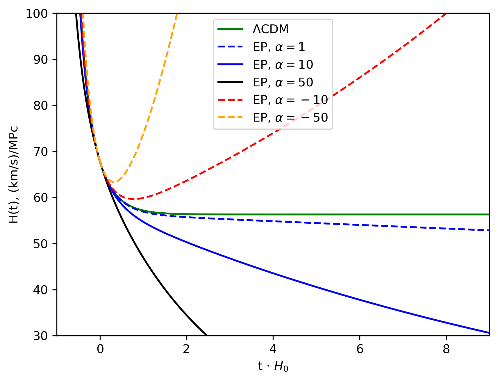
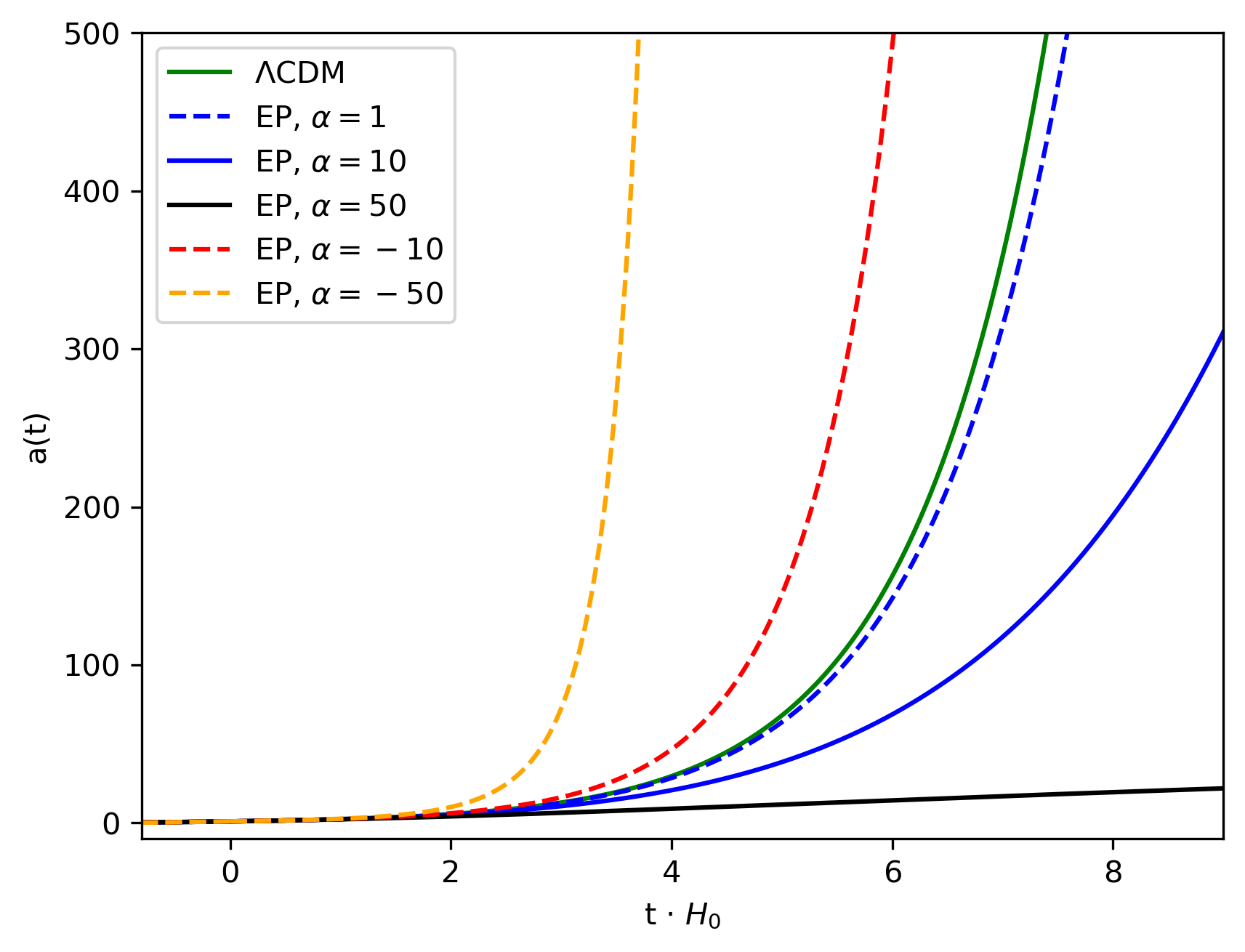
Figure 13: $H(t)$ vs $t\cdot H_{0}$ (left panel) and $a(t)$ vs $t\cdot H_{0}$ (right panel) for the exponential potential with $\alpha=1,10,50,-10,-50$.

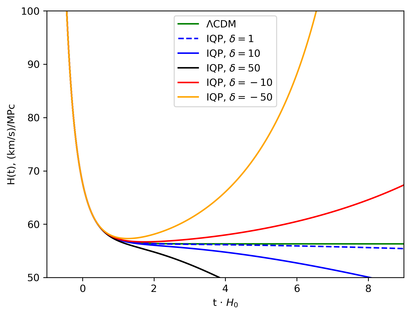
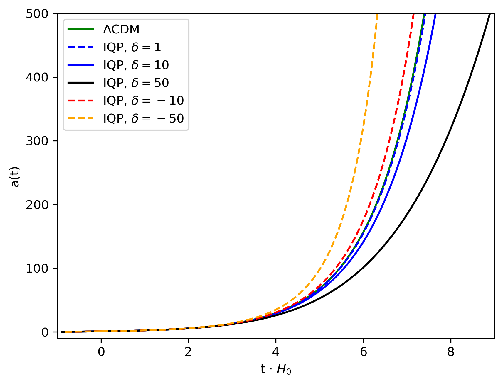
Figure 14: $H(t)$ vs $t\cdot H_{0}$ (left panel) and $a(t)$ vs $t\cdot H_{0}$ (right panel) for the inverse quartic potential with $\delta=1,10,50,-10,-50$.

5 Observational analysis

This section is devoted to explore the parameter space of the cosmological models proposed in section 4 using public available observational data. To this end, the Observational Hubble database from the cosmic chronometers [OHD, 30] and the Pantheon database from Supernova type Ia [PaSN, 31] are considered. The fit of the data is performed with a Bayesian statistical analysis using the algorithm called emcee [32], which implements an affine-invariant Markov Chain Monte Carlo (MCMC) sampler of the posterior distribution function (PDF) minimizing the following expression:

$$\ln\left(\mathcal{L}(\theta)\ \prod_{j}\mathcal{P}(\theta_{j})\right)\propto-\dfrac{\chi^{2}(\theta)}{2}+\sum_{j}\ln\left(\mathcal{P}(\theta_{j})\right)$$ (5.1)

where $\mathcal{L}(\theta)$ is the likelihood and $\mathcal{P}(\theta_{j})$ identifies the prior imposed on the $j$-th parameter. $\theta$ identifies the set of free parameters considered in the MCMC approach. The merit function, $\chi^{2}(\theta)$, depends on the differences between observed data (D) and model predictions ($\textbf{m}(\theta)$) over the redshift:

$$\chi^{2}(\theta)=\big{(}\textbf{D}-\textbf{m}(\theta)\big{)}^{T}\textbf{C}^{-1}\big{(}\textbf{D}-\textbf{m}(\theta)\big{)}$$ (5.2)

C being the noise covariance matrix of the observed data. In this notation, D and $\textbf{m}(\theta)$ are vectors while $\textbf{C}^{-1}$ is the inverse matrix of C. The value of each parameter and its uncertainty are obtained thought marginalization of the posterior distribution function of each parameter, as the median (the 50th percentile) and recovering the 16th and 84th percentiles to provide respectively the upper and lower uncertainties.

Each cosmological model is tested with three merit functions that depends on the data set considered, which are based on the observational Hubble data only (OHD, $\chi^{2}_{\rm OHD}$), on the Pantheon dataset data only (PaSNe, $\chi^{2}_{\rm SNIa}$) and on a combination of the two (OHD+PaSNe, $\chi^{2}_{\rm OHD+PaSNe}$). Concerning the simultaneous fit, the merit function is written as:

$$\chi^{2}_{\rm OHD+PaSNe}(\theta)=\chi^{2}_{\rm OHD}(\theta)+\chi^{2}_{\rm PaSNe}(\theta)$$ (5.3)

for which we assume that measurements from different databases are uncorrelated. Details about $\chi^{2}_{\rm OHD}$ and $\chi^{2}_{\rm PaSNe}$ are presented in the next sections.

5.1 Data and modelling

5.1.1 The Observational Hubble Database

The Observational Hubble Database, OHD, consists of 51 measurements of the Hubble parameter that covers the redshift range $0.07-2.36$ [30, 33]; which are obtained from the differential age method [DA, 34, 33] and from the baryon acoustic oscillation measurements. These OHD values can be compared directly with our proposed cosmological models that yield $H(z;\Theta)$ solving equations (4.3) and (4.4) (section 4), with $\Theta$ being the set of cosmological parameters that define our proposed models. Although some correlation are expected for the BAO measurements due of the overlapping among the galaxy samples or the cosmological model dependence in the clustering estimation [see discussion in 30], we follow previous work that assume no correlation between these measurements [e.g. see 35]. Therefore, the covariance noise matrix is diagonal (i.e. uncorrelated noise, $({\bf C}^{-1})_{i,j}=\delta_{i,j}/\sigma_{i}^{2}$), and consequently, the maximization of the posterior distribution is driven by the merit function:

$$\chi_{\rm OHD}^{2}(\theta)=\sum_{i=1}^{51}\left(\frac{H_{\textrm{obs},i}-H(z_{i};\theta)}{\sigma_{H_{\rm obs,i}}}\right)^{2}\,,$$ (5.4)

where $H_{\textrm{obs},i}$ and $\sigma_{H_{i}}$ are respectively the observed Hubble parameter and its uncertainty at redshift $z_{i}$ (OHD values). $H(z_{i};\theta)$ is the Hubble parameter provided by the model at the redshift $z_{i}$, with $\theta$ being the set of free parameters. In this case, $\theta$ corresponds to the set of cosmological parameters, i.e. $\theta=\Theta$. In our implementation, we applied the fourth-order Runge-Kutta method (RK4) to obtain the solution of $H(z_{i};\theta)$ for each point explored in the parameter space.

5.1.2 The Pantheon Supernovae Database

The Pantheon dataset, PaSNe, contains the apparent magnitude of 1048 SN Ia at the redshift range $0.01-2.3$ [31]. These observational measurements are fitted to the apparent magnitude model, $m_{b}(z_{i};\theta)$, which is written as [36, 37, 38, 39]:

$$m_{b}(z_{i};\theta)=5\log_{10}\left(D_{\rm L}(z_{i};\Theta)\right)+\mathcal{M}\,,$$ (5.5)

where $\mathcal{M}$ is considered a nuisance parameter that encompasses elements such as the absolute magnitude $\rm M_{\rm abs}$, which acts as a calibration term of the apparent magnitude of the SNIa sample [see details in 36, 37, 38, 39]. The (dimensionless) luminosity distance, $D_{\rm L}(z_{i};\Theta)$, depends on the cosmological model studied:

$$D_{\rm L}(z_{i};\Theta)=\frac{(1+z_{i})\ a_{0}H_{0}}{c}\ S_{k}\left(\frac{c}{a_{0}}\ \int_{0}^{z_{i}}\frac{dz^{\prime}}{H(z^{\prime};\Theta)}\right)\,,$$ (5.6)

where

$$S_{k}(x)=\left\{\begin{array}[]{rcl}\sin(x)\quad\text{for}\quad k&=&+1\\ x\quad\text{for}\quad k&=&0\\ \sinh(x)\quad\text{for}\quad k&=&-1\end{array}\right.$$ (5.7)

and $c$ is the speed of light. The variable $\Theta$ identifies the set of cosmological parameters of the proposed model. Similarly to the previous section, a numerical approach is taken into consideration to generate the model. We compute the numerical solution of $D_{\rm L}(z_{i};\Theta)$ for each $\Theta$ and $z_{i}$, for which the RK4 method is applied on Eqs. (4.3), (4.4) and on the derivative of the luminosity distance:

$$\frac{d}{dz}D_{\rm L}(z;\Theta)=\frac{D_{\rm L}(z;\Theta)}{1+z}+\frac{H_{0}\ (1+z)}{H(z;\Theta)}\sqrt{1+\Omega_{k,0}\left(\frac{\ D_{\rm L}(z;\Theta)}{\ (1+z)}\right)^{2}}\,,$$ (5.8)

that is valid for every value of $k$ ($k=-1,0,1$). Once achieved the solution of $D_{\rm L}(z_{i};\Theta)$ for each $z_{i}$, the apparent magnitude model is established with the set of free parameters $\theta=\{\Theta,\mathcal{M}\}$. Then, the merit function is given by:

$$\chi^{2}_{\rm PaSNe}(\theta)=\big{(}\mathbf{m}_{b,\rm obs}-\mathbf{m}_{b}(\theta)\big{)}^{T}\mathbf{C}^{-1}\big{(}\mathbf{m}_{b,\rm obs}-{\bf m}_{b}(\theta)\big{)}$$ (5.9)

where ${\bf m}_{b,\rm obs}$ and ${\bf m}_{b}(\theta)$ are vectors containing respectively the observed and theoretical apparent magnitudes of the whole SNe Ia sample. For the Pantheon measurements, the covariance matrix $\mathbf{C}$ depends on a statistical and on a systematic component describing the uncertainties; i.e. $\mathbf{C}=\mathbf{C}_{\rm stat}+\mathbf{C}_{\rm sys}$. The systematic uncertainties arise from the BEAMS method, which is applied to correct the bias that is generated by fits jointly nuisance parameters from the light curve of SNe Ia and the cosmological parameters [40]. Therefore, $\mathbf{C}_{\rm sys}$ also accounts for the correlation among the apparent magnitudes of the Pantheon dataset, i.e. the $\mathbf{C}_{\rm sys}$ is not a diagonal matrix: $({\bf C}_{\rm sys})_{i,j}\neq 0\ \forall\ i,j$. For an ideal case, if we assume that uncertainties are uncorrelated the noise covariance matrix becomes diagonal, so the merit function comes to take a simple shape:

$$\chi_{\rm PaSNe}^{2}(\theta)=\sum_{i=1}^{1048}\left(\frac{m_{\textrm{obs},i}-m_{b}(z_{i};\theta)}{\sigma_{m_{\textrm{obs},i}}}\right)^{2}\,,$$ (5.10)

where the uncertainty of each measurement is the contribution of the statistical and systematic uncertainties, i.e. $\sigma_{m_{\textrm{obs},i}}^{2}=\sigma_{m_{\textrm{stat},i}}^{2}+\sigma_{m_{\textrm{sys},i}}^{2}$.

5.1.3 Remarks on the fitting and analysis strategies

We investigate the cosmological models associated with the mimetic field potentials as outlined in section 4. The first family of models is characterized by an exponential potential $V(\phi)=V_{0}\,\rm{e}^{-\alpha\cdot\phi}$ (EP). We also consider a specific case with a fixed value of $\alpha=1$, $V(\phi)=V_{0}\,\rm{e}^{-\phi}$, which is denoted as EPf. The second family considers an inverse quartic potential $V(\phi)=V_{0}\,\left(1+\delta\cdot\phi^{2}\right)^{-2}$ (IQP). In particular, the case $\delta=1$ is identified as IQPf ($V(\phi)=V_{0}\,\left(1+\phi^{2}\right)^{-2}$). Table 5 provides a summary of the models, parameter space and datasets employed for each fit. The numerical solutions in section 4 indicate that for small values of $\alpha$ and $\delta$, the curves closely resemble the $\Lambda$CDM model for early times, as expected. As a preliminary approximation, we consider $\alpha=1$ and $\delta=1$ to assess how well these models align with the data and analyze the differences compared to $\Lambda$CDM. In this case, the reduced parameter space also leads to a shorter computational time. However, it is acknowledged that for extended times periods, all curves will deviate from $\Lambda$CDM. Subsequently, we will allow these parameters to be free, enabling a data-driven fitting process.

Since the MCMC performance requires of several iterations, the estimation of the all $H(z_{i};\theta)$ and $m_{b}(z_{i};\theta)$ models is computationally expensive. We therefore consider priors to expedite the characterization of the posterior distribution with the MCMC sampling approach. We consider two type of priors: $i)$ uniform priors, $\mathcal{U}(a,b)$, that follow a top-hat function in the interval $[a,b]$, and $ii)$ Gaussian priors, $\mathcal{N}(\overline{p},\sigma_{p})$, that follow a normal Gaussian distributions described by the mean and standard deviation of the $p$-parameter. The priors imposed on the free parameters are shown in Table 5. For instance, the uniform priors over $\Omega_{\phi,0}$ and $\Omega_{k,0}$ guarantee the physical meaning of these densities. In other cases, the Gaussian and uniform priors are useful to alleviate the exploration of the parameter space. For example, we use the same constraint imposed in Ref [38] for $\mathcal{M}$, this is $\mathcal{P}(\mathcal{M})=\mathcal{U}(23,24)$.

Once the priors are established, we run the emcee with 50 chains and 14000 iteration steps to characterize the posterior distributions of each case. The first 3500 steps are excluded of each chain (the burn-in sample). Overall, the parameters from the cosmological modeling are computed from the marginalized the posterior distribution function, PDF($\theta_{i}$), over each parameter $\theta_{i}$. Table 7 presents the parameters and their uncertainties, i.e. respectively the median and uncertainty (the 16th and 84th percentiles) of its PDF($\theta_{i}$), for all cases studied.

To assess the goodness of fits we provide the values of the chi-squared $\chi^{2}$ evaluated in the parameter space recovered and the reduced chi-squared $\chi_{\rm red}^{2}$ (accounting for the degrees of freedom). In addition, we can use statistical information criteria to determine whether the data favours one model over another. We selected two standard statistical indicators: 1) the Akaike Information Criterion [AIC, 41], and 2) the Bayesian Information Criterion [BIC, 42]. They are computed from the following expressions:

$${\rm AIC}=2\,N_{\theta}-2\ln\,(\mathcal{L}_{\rm max})\ \ {\rm and}\ \ {\rm BIC}=N_{\theta}\ln\,(n)-2\ln\,(\mathcal{L}_{\rm max})$$ (5.11)

where $N_{\theta}$ corresponds to the number of free parameters of the model, $\mathcal{L}_{\rm max}$ is the value of the likelihood function evaluated at the best fit, and $n$ corresponds to the sample size. In the case of asymmetric distributions, where the median departs from the peak of the posterior, we use the latter to maintain the meaning of the definition of AIC and BIC. In our case, we have respectively $n_{\rm OHD}=51$ and $n_{\rm PaSNe}=1048$ for the OHD and Pantheon cases, which corresponds to $n_{\rm OHD+PaSNe}=1099$ for the joint analysis. These statistical quantities are confronted with those values obtained for the $\Lambda$CDM fits with curvature assumption cases, which are computed as:

$$\rm\Delta\,AIC_{model}=AIC_{model}-AIC_{\Lambda CDM}\ \ and\ \ \Delta\,BIC_{model}=BIC_{model}-BIC_{\Lambda CDM}.$$ (5.12)

with “model” being the identification name of the model considered. $\rm\Delta\,AIC_{model}$ and $\rm\Delta\,BIC_{model}$ are computed with respect to fits that use the same database. The AIC, BIC, $\rm\Delta\,AIC_{model}$ and $\rm\Delta\,BIC_{model}$ are also listed in Table 7.

As a consistent test, the $\Lambda$CDM model for a flat universe is studied in order to compare the performance of our methodology with respect to literature analysis. We follow [35] and fit the three data sets to the $\Lambda$CDM model (assuming a flat universe) with the prior $\mathcal{P}(H_{0})=\mathcal{N}(73.24,1.74)$, where the parameter space consists of $\theta=\{\Omega_{\phi,0},H_{0}\}$ for the OHD case and $\theta=\{\Omega_{\phi,0},H_{0},\mathcal{M}\}$ for the PaSNe and OHD+PaSNe cases. For all analyses, the $H_{0}$ and $\Omega_{\phi,0}$ recovered are in full agreement with the results obtained by [35]. As an example, we obtained $H_{0}=70.51^{+0.85}_{-0.86}$ $\rm km\,s^{-1}\,Mpc^{-1}$ and $\Omega_{\phi,0}=0.265\pm 0.013$ for the OHD+PaSNe case, while they reported $H_{0}=70.5\pm 0.9$ $\rm km\,s^{-1}\,Mpc^{-1}$ and $\Omega_{\phi,0}=0.265^{+0.013}_{-0.012}$ (see Table I in [35]). This confirms that our methodology is a reliable and robust approach.

Model ID	Potential	Parameter space for non-flat models
		$\theta_{\rm OHD}=\{H_{0},\Omega_{\phi,0},\Omega_{k,0},\alpha\}$
EP	$V(\phi)=V_{0}\,\rm{e}^{-\alpha\cdot\phi}$	$\theta_{\rm PaSNe}=\{H_{0},\Omega_{\phi,0},\Omega_{k,0},\alpha,\mathcal{M}\}$
		$\theta_{\rm OHD+PaSNe}=\{H_{0},\Omega_{\phi,0},\Omega_{k,0},\alpha,\mathcal{M}\}$
		$\theta_{\rm OHD}=\{H_{0},\Omega_{\phi,0},\Omega_{k,0}\}$
EPf	$V(\phi)=V_{0}\,\rm{e}^{-\phi}$	$\theta_{\rm PaSNe}=\{H_{0},\Omega_{\phi,0},\Omega_{k,0},\mathcal{M}\}$
		$\theta_{\rm OHD+PaSNe}=\{H_{0},\Omega_{\phi,0},\Omega_{k,0},\mathcal{M}\}$
		$\theta_{\rm OHD}=\{H_{0},\Omega_{\phi,0},\Omega_{k,0},\delta\}$
IQP	$V(\phi)=V_{0}\,\left(1+\delta\cdot\phi^{2}\right)^{-2}$	$\theta_{\rm PaSNe}=\{H_{0},\Omega_{\phi,0},\Omega_{k,0},\delta,\mathcal{M}\}$
		$\theta_{\rm OHD+PaSNe}=\{H_{0},\Omega_{\phi,0},\Omega_{k,0},\delta,\mathcal{M}\}$
		$\theta_{\rm OHD}=\{H_{0},\Omega_{\phi,0},\Omega_{k,0}\}$
IQPf	$V(\phi)=V_{0}\,\left(1+\phi^{2}\right)^{-2}$	$\theta_{\rm PaSNe}=\{H_{0},\Omega_{\phi,0},\Omega_{k,0},\mathcal{M}\}$
		$\theta_{\rm OHD+PaSNe}=\{H_{0},\Omega_{\phi,0},\Omega_{k,0},\mathcal{M}\}$
Priors	$\mathcal{P}(H_{0}):\ \mathcal{U}(0,100)$ and $\mathcal{N}(73.24,5)$ $\rm(km\,s^{-1}Mpc^{-1})$
	$\mathcal{P}(\Omega_{\phi,0})=\mathcal{U}(0,1)$ and $\mathcal{N}(0.73,0.05)$
	$\mathcal{P}(\Omega_{k,0}):\ \mathcal{U}(-0.2,0.2)$, $\mathcal{P}(\alpha)=\mathcal{U}(-50,50)$
	$\mathcal{P}(\delta)=\mathcal{U}(-1000,\infty)$, and $\mathcal{P}(\mathcal{M})=\mathcal{U}(23,24)$

Table 5: Models, parameter spaces and priors considered in this work.

Dataset	$\Omega_{\phi,0}$	$\alpha$	$\delta$	$\Omega_{k,0}$	$H_{0}$	$\mathcal{M}$	$\chi_{\rm min}^{2}$	$\chi_{\rm red}^{2}$	AIC	BIC	$\Delta\,{\rm AIC}$	$\Delta\,{\rm BIC}$
$\Lambda$CDM
OHD	$0.707\pm 0.045$	$-$	$-$	$0.047\pm 0.058$	$70.23^{+1.26}_{-1.21}$	$-$	$26.5$	$0.55$	$32.5$	$38.3$	$-$	$-$
PaSNe	$0.730^{+0.043}_{-0.045}$	$-$	$-$	$-0.047^{+0.077}_{-0.075}$	$73.41^{+4.89}_{-5.04}$	$23.81\pm 0.01$	$1027.2$	$0.98$	$1035.2$	$1055.0$	$-$	$-$
OHD+PaSNe	$0.691\pm 0.039$	$-$	$-$	$0.051^{+0.055}_{-0.054}$	$69.39^{+1.00}_{-0.98}$	$23.80\pm 0.01$	$1055.0$	$0.96$	$1063.0$	$1083.0$	$-$	$-$
EP
OHD	$0.715\pm 0.042$	$-11.94^{+34.53}_{-25.31}$	$-$	$0.082^{+0.078}_{-0.129}$	$70.34^{+1.35}_{-1.29}$	$-$	$26.4$	$0.56$	$34.4$	$42.1$	$1.9$	$3.8$
PaSNe	$0.727^{+0.041}_{-0.042}$	$-2.54^{+32.09}_{-31.21}$	$-$	$-0.041^{+0.099}_{-0.093}$	$73.35^{+4.88}_{-5.06}$	$23.81\pm 0.01$	$1026.9$	$0.98$	$1036.9$	$1061.7$	$1.7$	$6.7$
OHD+PaSNe	$0.699^{+0.037}_{-0.038}$	$18.08^{+19.00}_{-27.50}$	$-$	$-0.020^{+0.117}_{-0.104}$	$69.49^{+1.01}_{-0.99}$	$23.81\pm 0.01$	$1055.0$	$0.96$	$1065.0$	$1090.0$	$2.0$	$7.0$
EPf
OHD	$0.706^{+0.045}_{-0.044}$	$-$	$-$	$0.045\pm 0.058$	$70.20^{+1.24}_{-1.21}$	$-$	$26.5$	$0.55$	$32.5$	$38.3$	$0$	$0$
PaSNe	$0.730^{+0.043}_{-0.044}$	$-$	$-$	$-0.051^{+0.077}_{-0.072}$	$73.29^{+4.88}_{-5.01}$	$23.81\pm 0.01$	$1027.0$	$0.98$	$1035.0$	$1054.8$	$-0.2$	$-0.2$
OHD+PaSNe	$0.692\pm 0.039$	$-$	$-$	$0.047^{+0.054}_{-0.055}$	$69.41^{+1.01}_{-0.98}$	$23.80\pm 0.01$	$1054.9$	$0.96$	$1062.9$	$1082.9$	$-0.1$	$-0.1$
IQP
OHD	$0.717^{+0.042}_{-0.043}$	$-$	$1568.9^{+2644.8}_{-1859.9}$	$0.116^{+0.061}_{-0.095}$	$71.03^{+1.65}_{-1.53}$	$-$	$29.1$	$0.62$	$37.1$	$44.8$	$4.6$	$6.5$
PaSNe	$0.725^{+0.042}_{-0.041}$	$-$	$7012.1^{+10114.6}_{-5753.0}$	$0.063^{+0.092}_{-0.110}$	$73.88^{+4.89}_{-4.95}$	$23.80\pm 0.01$	$1027.8$	$0.99$	$1037.8$	$1062.6$	$2.6$	$7.6$
OHD+PaSNe	$0.696\pm 0.041$	$-$	$-368.8^{+970.0}_{-469.5}$	$0.035^{+0.074}_{-0.069}$	$69.41^{+1.00}_{-0.97}$	$23.80\pm 0.01$	$1054.5$	$0.96$	$1064.5$	$1089.5$	$1.5$	$6.5$
IQPf
OHD	$0.707\pm 0.045$	$-$	$-$	$0.048^{+0.058}_{-0.057}$	$70.23^{+1.27}_{-1.22}$	$-$	$26.5$	$0.55$	$32.5$	$38.3$	$0$	$0$
PaSNe	$0.730^{+0.043}_{-0.044}$	$-$	$-$	$-0.048^{+0.077}_{-0.074}$	$73.27^{+5.01}_{-4.98}$	$23.81\pm 0.01$	$1027.1$	$0.98$	$1035.1$	$1054.9$	$-0.1$	$-0.1$
OHD+PaSNe	$0.692\pm 0.039$	$-$	$-$	$0.050\pm 0.054$	$69.41^{+1.00}_{-0.99}$	$23.80\pm 0.01$	$1054.9$	$0.96$	$1062.9$	$1082.9$	$-0.1$	$-0.1$

Table 6: Parameters and uncertainties obtained for the non-flat cosmological models investigated. The identification names and field potentials for the $\Lambda$CDM model and mimetic gravity models (EP, EPf, IQP and IQPf) are listed in Table 5. The properties of these non-flat cosmological models are obtained using three data set: the observational Hubble database from the cosmic chronometers (OHD), the Pantheon database from Supernova type Ia (PaSNe) and the simultaneous analysis of the OHD and PaSNe data sets (OHD+PaSNe). The statistical parameters $\Delta\rm AIC$ and $\Delta\rm BIC$ are computed with respect to the non-flat $\Lambda$CDM results for the same database.

5.2 Cosmological constraints

We provide the properties of non-flat cosmological models obtained with the three datasets (Table 7). We investigate the marginalized posteriors and corner plots (the 2D contours of the PDFs) for the $\Lambda$CDM (Fig. 15), EP (Figs. 16 and 17) and IQP (Figs. 18 and 19) cosmological models with spatial curvature. Overall, the non-flat cosmological models do not show substantial statistical preference over the base $\Lambda$CDM, EP, IQP models with the assumption of a flat universe, $\Omega_{k,0}=0$. For example, the OHD+PaSNe analysis provide $\Omega_{k,0}$ values of $0.051^{+0.055}_{-0.054}$ ($\Lambda$CDM), $-0.020^{+0.117}_{-0.104}$ (EP) and $0.035^{+0.074}_{-0.069}$ (IQP) which are consistent with a flat universe. As reference, the results for the flat universe scenario are presented in appendix F.

We consider the OHD+PaSNe analysis as our reference modeling because it considers both data sets at the same time, which allow us to access more cosmological information. In spite of this, the goodness-of-fit appears to be better for the OHD cases, with $\chi^{2}_{\rm red}$ around 0.55 for all models tested (Table 7). Although, this low value also could reflect that the uncertainties of the observational measurements are underestimated. In contrast, the OHD+PaSNe and PaSNe analysis respectively provide $\chi^{2}_{\rm red}$ of 0.96 and $\sim 0.98$. We therefore confirm the performance of the fits is robust and similar when the same data set is considered.

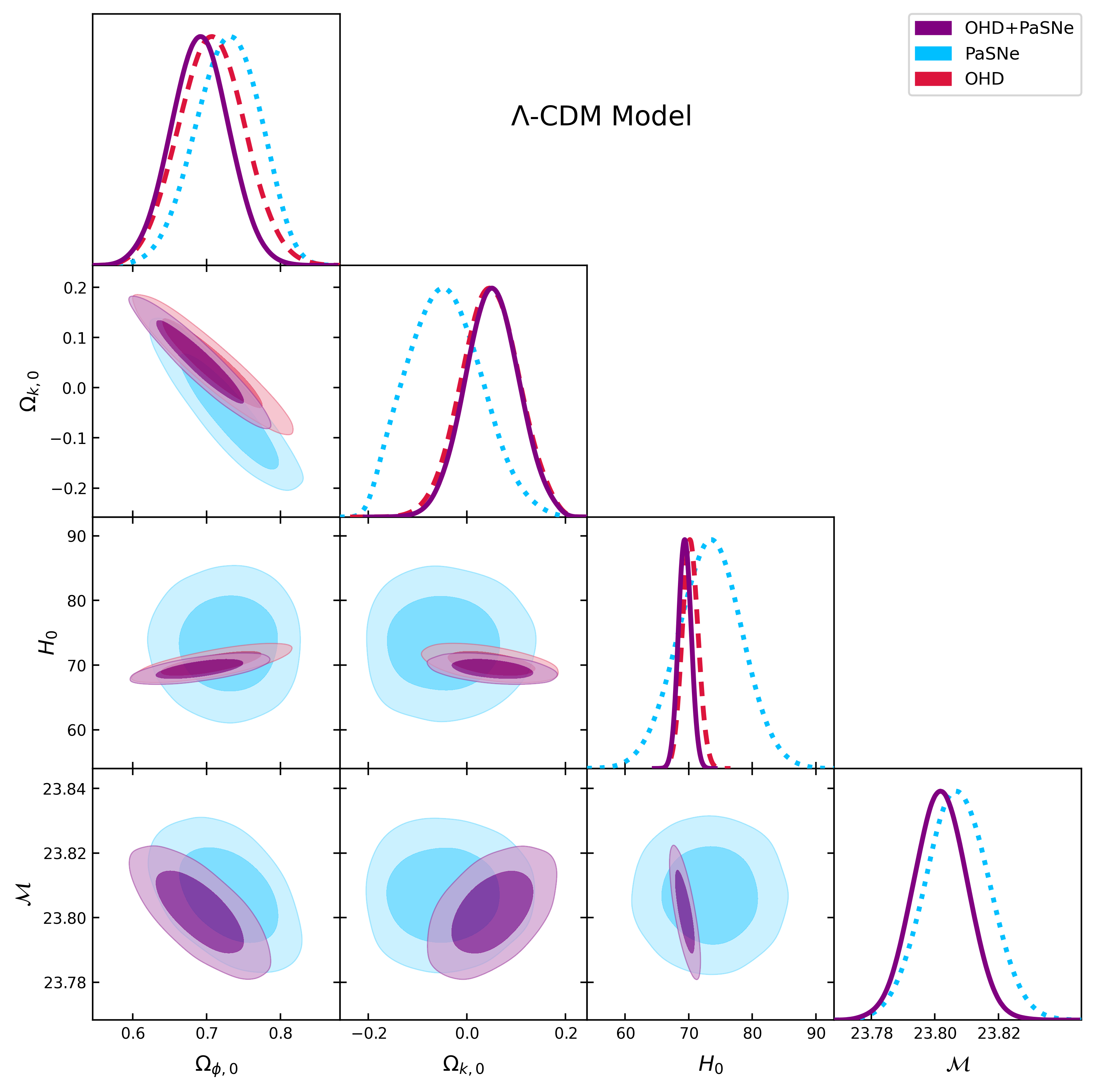
Figure 15: Marginalized posteriors and correlation plots for the parameters $\Omega_{\phi,0}$, $\Omega_{k,0}$, $H_{0}$, $\mathcal{M}$ that describe the non-flat $\Lambda$CDM model. The contours represent the 68.3% and 95.4% confidence levels. The results obtained from the OHD+PaSNe, PsSNe and OHD analysis, Table 7, are identified respectively by the purple, blue and red colors. $H_{0}$ is in units of $\rm km\,s^{-1}\,Mpc^{-1}$, while $\Omega_{\phi,0}$, $\Omega_{k,0}$ and $\mathcal{M}$ are dimensionless units.

Regarding the curved universe scenarios, the $\Omega_{k,0}$ values are compatible with zero for all cases studied, with the significance of detection being around one (see Table 7). Overall, the OHD and OHD+PaSNe analysis prefer positive curvature in contrast to the PaSNe fits. Only the IQP modeling shows positive curvature values for the three data sets. The non-flat $\Lambda$CDM scenario yields $\Omega_{k,0}$ of $0.047\pm 0.058$, $-0.047^{+0.077}_{-0.075}$ and $0.051^{+0.055}_{-0.054}$ for the OHD, PaSNe and OHD+PaSNe fits, respectively. Despite our higher uncertainties, these values are compatible with literature. For example, [43] obtained $\Omega_{k,0}$ between $-0.043$ up to 0.0008 using the CMB temperature and polarization power spectra (TT, TE and EE), BAO and the Pantheon sample for the base $\Lambda$CDM with spatial curvature. The CMB data alone have provided significance between 2 up to $3\sigma$ that depart from the $\Omega_{k,0}=0$ scenario [44, 45, 46, and reference therein]; for example, $\Omega_{k,0}=-0.044^{+0.018}_{-0.019}$ was obtained from the Planck data [47]. Although the new analysis of the Planck data have allowed to achieve stronger constraints such as $-0.025^{+0.013}_{-0.010}$ [48] and $-0.012\pm 0.010$ [49]. Including the CMB data is beyond the scope of this work, although this is one of the goals of a future work.

For the PaSNe fits, we also observe that negative values of $\Omega_{k,0}$ are associated to high values of the $H_{0}$ ($\sim 73.4\,\rm km\,s^{-1}\,Mpc^{-1}$) and $\Omega_{\phi,0}$ ($\sim 0.73$) parameters, except to the EPf model where $\Omega_{k,0}>0$. The correlation between them is not clear in the corner plots (see the blue 2D-PDFs of $\Omega_{k,0}$ versus $H_{0}$ and $\Omega_{\phi,0}$). However, the OHD+PaSNe analysis show a anti-correlation between $\Omega_{k,0}$ and $H_{0}$. This is in opposite direction when the CMB data is considered, which provides larger values of $\Omega_{k,0}$ as $H_{0}$ increases; e.g see [4, 48, 49] for only CMB data. Previous works also reported higher values of $H_{0}$ when only the type Ia supernovae data is considered [e.g., 35, 50, 51, 52]. For instance, [35] obtained respectively values of $H_{0}$ of $73.2\pm 1.7$ and $70.5\pm 0.9\,\rm km\,s^{-1}\,Mpc^{-1}$ for their SNe Ia and Joint (similar to our PSNe and OHD+PSNe) fits for the $\Lambda$CDM model. They also reported this trend for their four models studied [see Table I in 35]. For non-flat Universes, for example, [43] observed lower values of $H_{0}$ for the CMB+PaSNe dataset with respect to fits considering the CMB+BAO and CMB+PaSNe+BAO for all model investigated, where the CMB+PaSNe cases always provided $\Omega_{k}<0$. This change in trend could be connected with the inclusion of the CMB data (temperature and polarization power spectra).

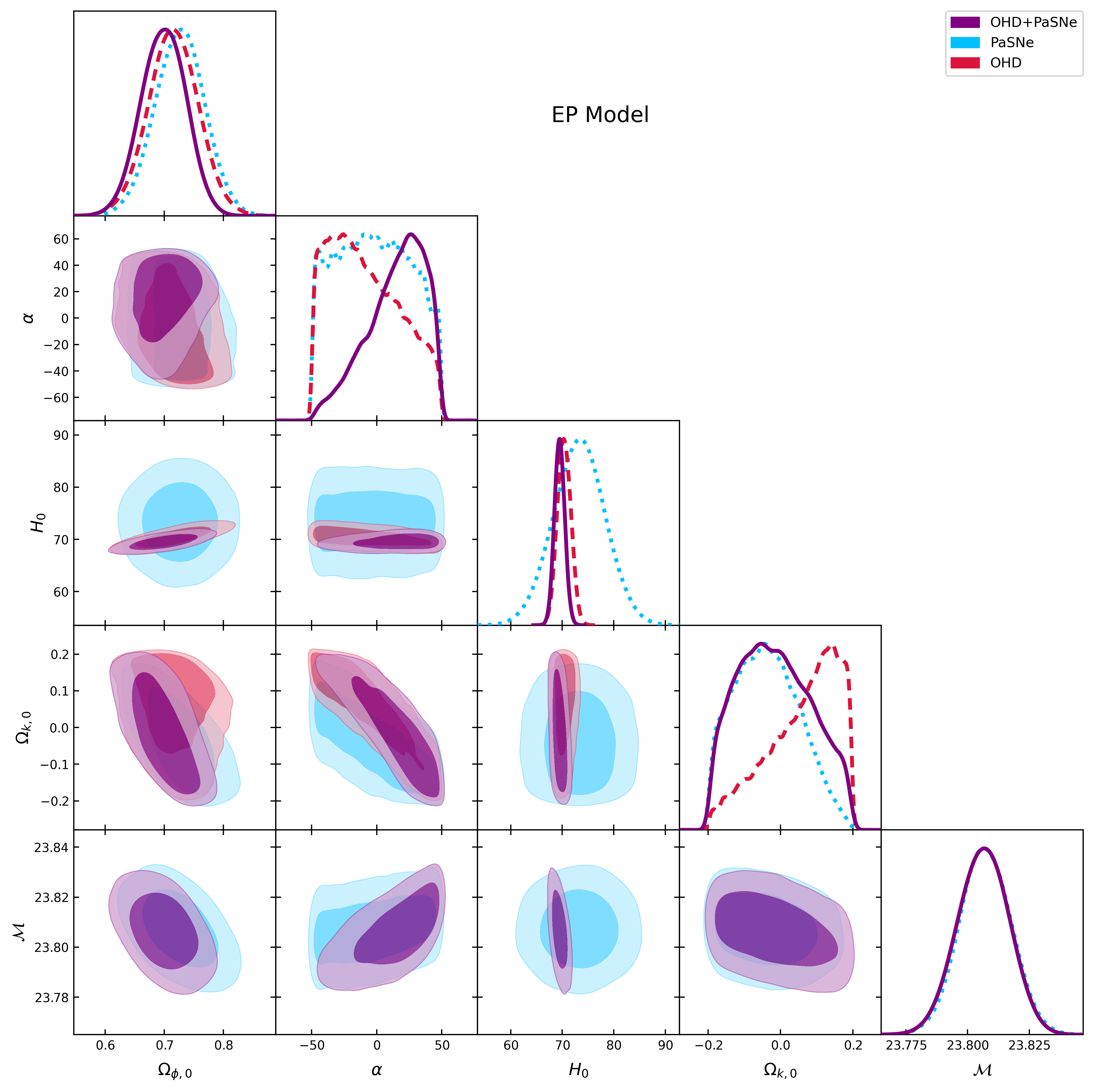
Figure 16: Marginalized posteriors and correlation plots for the parameters $\Omega_{\phi,0}$, $\alpha$, $\Omega_{k,0}$, $H_{0}$, $\mathcal{M}$ that describe the EP model (the exponential potential) with spatial curvature. The contours represent the 68.3% and 95.4% confidence levels. The results obtained from the OHD+PaSNe, PsSNe and OHD analysis, Table 7, are identified respectively by the purple, blue and red colors. $H_{0}$ is in units of $\rm km\,s^{-1}\,Mpc^{-1}$, while $\Omega_{\phi,0}$, $\alpha$, $\Omega_{k,0}$ and $\mathcal{M}$ are dimensionless units.

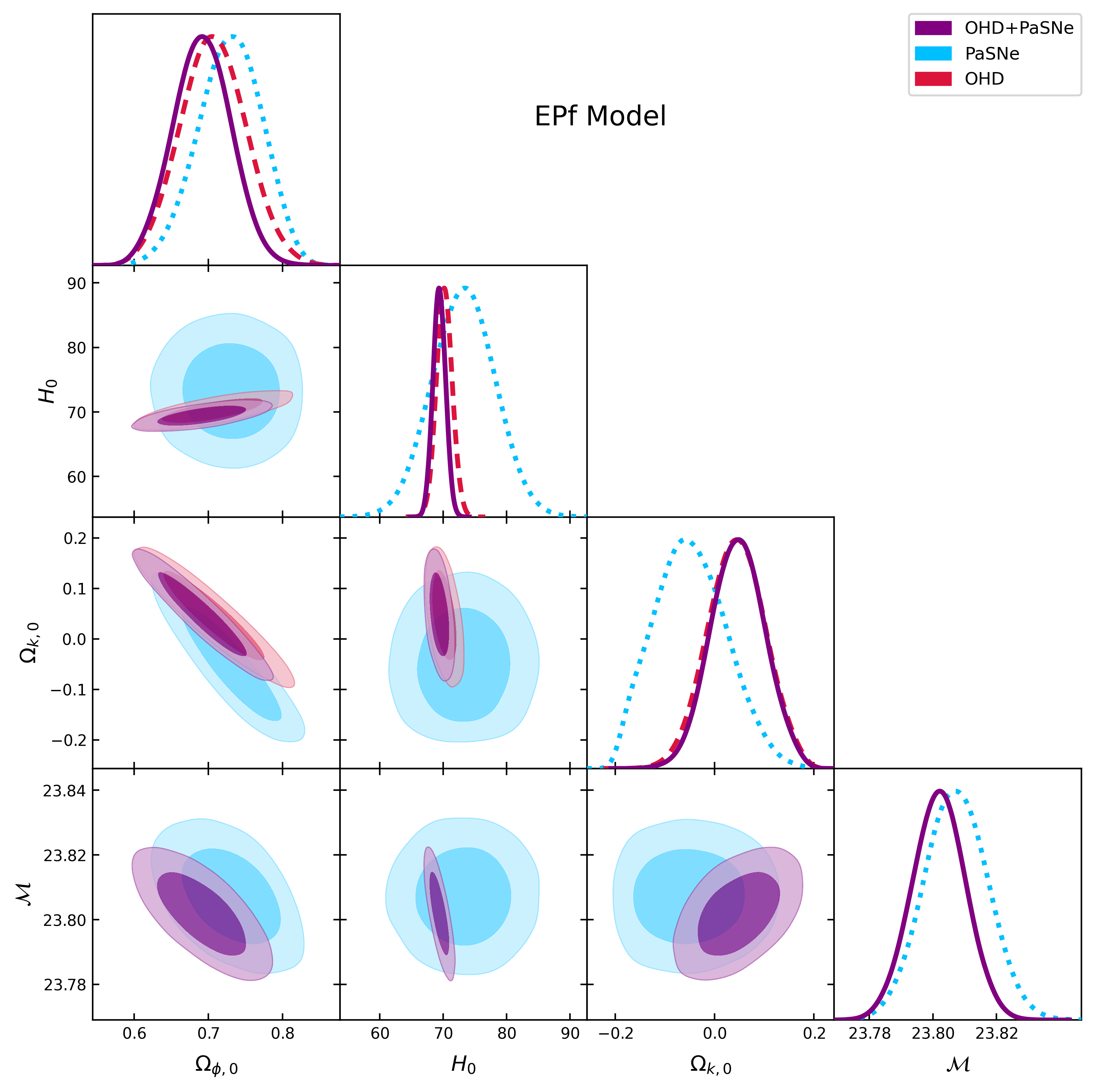
Figure 17: Marginalized posteriors and correlation plots for the parameters $\Omega_{\phi,0}$, $\alpha$, $\Omega_{k,0}$, $H_{0}$, $\mathcal{M}$ that describe the EPf model (the exponential potential with $\alpha=1$) with spatial curvature. The contours represent the 68.3% and 95.4% confidence levels. The results obtained from the OHD+PaSNe, PsSNe and OHD analysis, Table 7, are identified respectively by the purple, blue and red colors. $H_{0}$ is in units of $\rm km\,s^{-1}\,Mpc^{-1}$, while $\Omega_{\phi,0}$, $\alpha$, $\Omega_{k,0}$ and $\mathcal{M}$ are dimensionless units.

5.2.1 Non-flat Exponential Potential models

Regarding the EP model, the $\Omega_{\phi,0}$, $H_{0}$ and $\mathcal{M}$ recovered are in agreement with the obtained for the non-flat $\Lambda$CDM analyses (for all cases). These are performed with very similar goodness-of-fit (see Table 7), providing a $\chi^{2}$ of 0.96 for both non-flat $\Lambda$CDM and EP models (OHD+PaSNe case). Although we obtained a relatively high $\Delta\rm BIC=7$ and moderate $\Delta\rm AIC=2$, which favours the non-flat $\Lambda$CDM over the EP models. The OHD+PaSNe analysis provides an $\Omega_{k,0}=-0.02^{+0.12}_{-0.104}$ that contrasts with the positive curvature from the non-flat $\Lambda$CDM model ($\Omega^{\rm\Lambda CDM}_{k,0}=0.051^{+0.055}_{-0.054}$), although they are still consistent and compatible with zero at one-$\sigma$. In addition, we observed asymmetric PDFs for $\Omega_{k,0}$ and their behaviors depend on the data used. The marginalized PDFs reach their maximum at around $-0.01$ (OHD+PaSNe and PaSNe) and 0.013 (OHD), respectively. We also obtained that $\alpha$ is described by asymmetric marginalized PDFs and the high dispersion does not allow a good constraints on $\alpha$. For the OHD+PaSNe and OHD cases, their PDFs are peaking at around 25 and $-30$, respectively. In contrast, the PDF of $\alpha$ is poorly characterized for the PaSNe data yielding $\alpha=3\pm 32$. We therefore obtained a wide range of values of $\alpha$ that follows the imposed uniform prior ranging from $-50$ to 50, with $\alpha=18^{+19}_{-28}$ (OHD+PaSNe) being the most restrictive value. This is a poor constraint on $\alpha$, which can increase the degeneracy between other parameters of the EP model.

The contour plot between $\alpha$ and $\Omega_{k,0}$ shows an anti-correlation (see Fig. 16), where the extended tails are slightly shifted to negative and positive values of $\Omega_{k,0}$ and $\alpha$, respectively. For other 2D contours, we did not observe a significant change with respect to the non-flat $\Lambda$CDM. For instance, the $\Omega_{\phi,0}-\Omega_{k,0}$ PDFs appear to be broader than the the non-flat $\Lambda$CDM cases. This suggests that the $\alpha-\Omega_{k,0}$ anti-correlation could be independent of other parameters, although we must keep in mind that $\alpha$ is poorly characterized.

To avoid the effects of consider $\alpha$ as free parameter, we explored the EP model with $\alpha=1$ (called EPf, Fig. 17). This case provides results more consistent with the $\Lambda$CDM than to those from the EP model. For instance, the OHD+PaSNe case is performed with $\chi^{2}_{\rm red}=0.96$ for both non-flat $\Lambda$CDM and EPf models, with $\Delta\rm AIC=-0.1$ and $\Delta\rm BIC=-0.1$ that in a negligible level favor the EPf results. We recover a positive curvature $\Omega_{k,0}=0.047^{+0.054}_{-0.055}$, $H_{0}=69.4\pm 1.0\,\rm km\,s^{-1}\,Mpc^{-1}$ and $\Omega_{\phi,0}=0.692\pm 0.039$. In addition, the EPf model prefers positive $\Omega_{k,0}$ at 0.8$\sigma$, in contrast to the negative curvature at $1.7\sigma$ from the EP model which is slightly more shifted towards $\Omega_{k,0}=0$. Moreover, the marginalized PDFs of $\Omega_{k,0}$ are symmetrical and become more sharpened than in the cases of the EP analysis. These two features are also extended to the behaviour of the 2D contours for $\Omega_{\phi,0}-\Omega_{k,0}$, which now are more compatible with the corner plots from the non-flat $\Lambda$CDM analysis.

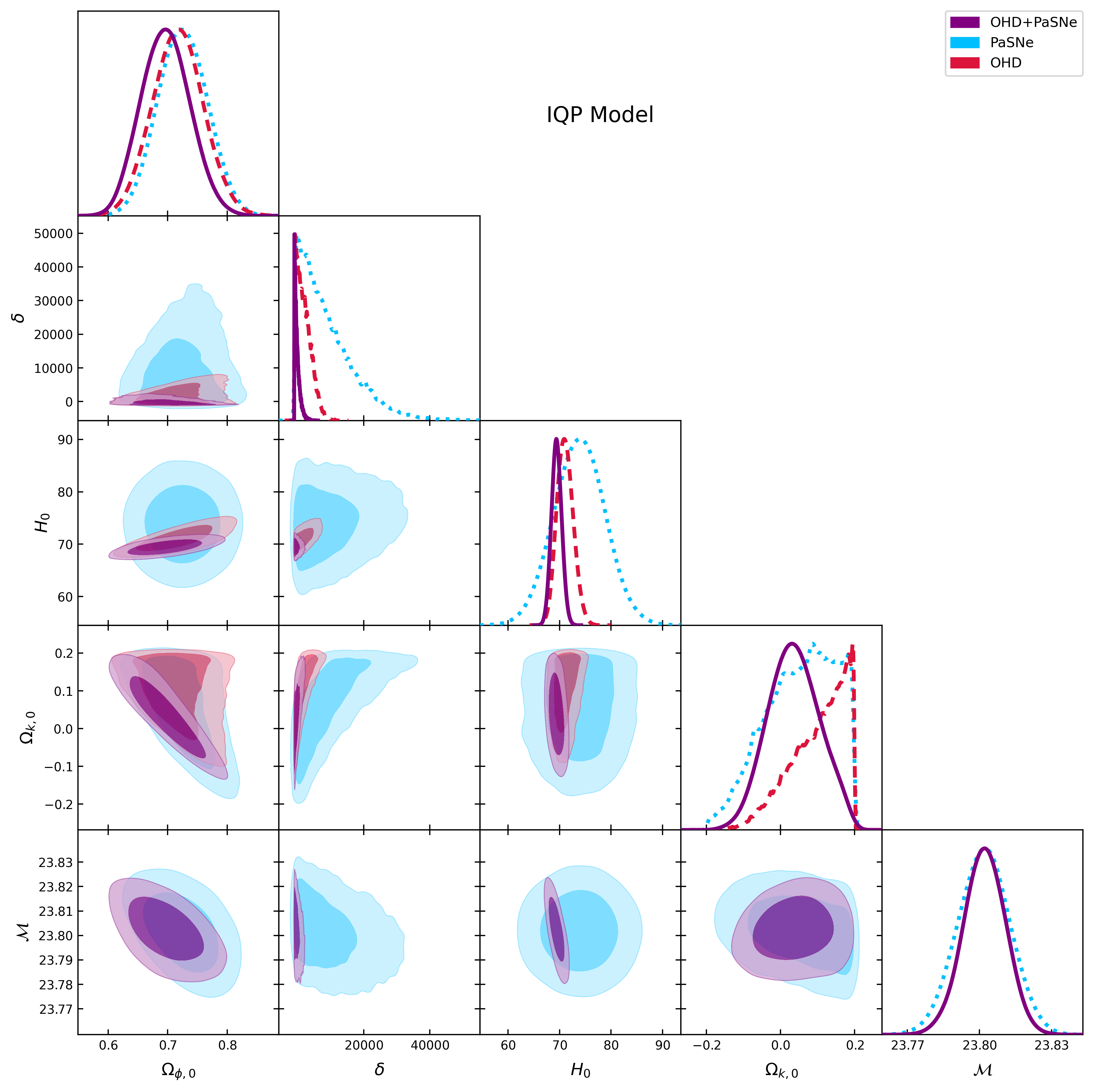
Figure 18: Marginalized posteriors and correlation plots for the parameters $\Omega_{\phi,0}$, $\delta$, $\Omega_{k,0}$, $H_{0}$, $\mathcal{M}$ that describe the IQP model (the inverse quadratic potential) with spatial curvature. The contours represent the 68.3% and 95.4% confidence levels. The results obtained from the OHD+PaSNe, PsSNe and OHD analysis, Table 7, are identified respectively by the purple, blue and red colors. $H_{0}$ is in units of $\rm km\,s^{-1}\,Mpc^{-1}$, while $\Omega_{\phi,0}$, $\delta$, $\Omega_{k,0}$ and $\mathcal{M}$ are dimensionless units.

Figure 19: Marginalized posteriors and correlation plots for the parameters $\Omega_{\phi,0}$, $\Omega_{k,0}$, $H_{0}$, $\mathcal{M}$ that describe the IQPf model (the inverse quadratic potential with $\delta=1$) with spatial curvature. The contours represent the 68.3% and 95.4% confidence levels. The results obtained from the OHD+PaSNe, PsSNe and OHD analysis, Table 7, are identified respectively by the purple, blue and red colors. $H_{0}$ is in units of $\rm km\,s^{-1}\,Mpc^{-1}$, while $\Omega_{\phi,0}$, $\Omega_{k,0}$ and $\mathcal{M}$ are dimensionless units.

5.2.2 Non-flat Inverse Quartic Potential models

Similar to the EP model, the parameters ($\Omega_{\phi,0}$, $H_{0}$ and $\mathcal{M}$) and goodness-of-fits obtained from the IQP models agree with the results from the non-flat $\Lambda$CDM analyses (see Fig. 18). For the OHD+PaSNe, the $\chi^{2}=0.96$ is the same for both non-flat $\Lambda$CDM and IQP models, yielding $\Omega_{k,0}=0.035^{+0.074}_{-0.069}$, $H_{0}=69.4\pm 1.0\,\rm km\,s^{-1}\,Mpc^{-1}$ and $\Omega_{\phi,0}=0.696\pm 0.041$. The positive curvature moves slightly (with respect to the non-flat $\Lambda$CDM model) towards $\Omega_{k,0}=0$ at a level of $0.5\sigma$, although the uncertainty is broader in the IQP model. In addition, the $\Delta\rm BIC=6.6$ and moderate $\Delta\rm AIC=1.5$ favors the non-flat $\Lambda$CDM over the IQP models with freely sampled of $\delta$.

The marginalized PDFs of $\delta$ are asymmetrical, particularly for the OHD and PaSNe cases, with tails extending up to unreasonable values of 40000 in the worst case. We therefore can provide only a weak description of the $\delta$. The sharper PDF results from the OHD+PaSNe case, even though its peak is located near to the lower bound of the uniform prior imposed on $\delta$. In addition, the OHD and PaSNe analysis also show a significant impact on the shape of the $\Omega_{k,0}$ PDFs, mainly owing to the irregular description of the $\delta$ parameter. For the OHD analysis, the peak of the PDF reaches the upper bound of the uniform prior imposed on $\Omega_{k,0}$, while the curve is wider for the PaSNe case and peaking around 0.1. We need a more restrictive prior to evaluate possible correlation among $\delta$ and other parameters such $\Omega_{k,0}$ (similarly to the EP analysis).

For the case with $\delta=1$ (IQPf), we obtained a parameter space in full agreement with the non-flat $\Lambda$CDM results, where the goodness-of-fit and comparison parameters ($\Delta\rm BIC$ and $\Delta\rm AIC$) are practically equals for each database that explore both models (Table 7). For example, the OHD+PaSNe case is performed with $\chi^{2}_{\rm red}=0.96$ for both non-flat $\Lambda$CDM and IQPf models, with $\Delta\rm AIC=-0.1$ and $\Delta\rm BIC=-0.1$ favoring (in a negligible level) the IQPf results. The IQPf analysis provide sharper and more symmetrical PDFs behaviour than the IQP model analysis (see Fig. 19). Also the correlation plots are now well delimited (with respect to the IQP models). The PDFs of $\Omega_{k,0}$ are described inside the range of the uniform prior considered for $\Omega_{k,0}$. In particular, the OHD and PaSNe curves are not reaching the prior upper limits as their maximum. For example, in the OHD case, the peak is now at $\Omega_{k,0}\approx 0.48$ in contrasted to the value of -0.2 from the IQP model. For the OHD+PaSNe analysis, we obtained $\Omega_{k,0}=0.050\pm 0.054$, $H_{0}=69.4\pm 1.0\,\rm km\,s^{-1}\,Mpc^{-1}$ and $\Omega_{\phi,0}=0.692\pm 0.039$, which is compatible with the non-flat $\Lambda$CDM results and with a flat universe.

6 Conclusions

We presented a dynamic description of the isotropic and homogeneous Friedmann-Lematre-Robertson-Walker cosmological models, with positive spatial curvature within the framework of mimetic gravity theory. We consider families of specific mimetic field potentials: the exponential potential (EP), the inverse square potential (ISP) and the inverse quartic potential (IQP). In addition, the parameters of the EP and IQP models were fitted with observational data from the Pantheon database of Supernovae type Ia and the Observational Hubble database from cosmic chronometers.

First, we considered a generic potential for the mimetic field and determined the critical points of the dynamical system. We analyzed the stability of each of them using linear stability and the centre manifold method for cases with null eigenvalues of the variation matrix. To understand the dynamics of the system at infinity, we studied the global phase space of the dynamical system by projecting on the Poincaré sphere. The dynamical system is four-dimensional, with the exception of the ISP ($V(\phi)\propto 1/\phi^{2}$) for which the dimension reduces to three. We explored the dynamics on invariant submanifolds, revealing trajectories that can evolve to a de Sitter universe and a division of the phase space in contracting and expanding epochs.

For the ISP ($V=\gamma/\phi^{2}$), the dynamical system reduced to a three-dimensional autonomous system. Trajectories starting from the matter dominated critical line could evolve towards a future attractor representing a solution dominated by dark matter and dark energy, exhibiting acceleration under certain conditions. Additionally, we identified trajectories that can enter the contracting phase space and recollapse to a big crunch. The phase space of this potential do not include the solution representing Einstein static universe. On the other hand, for the EP ($V=V_{0}e^{-\alpha\phi}$) we found that one equation decouples from the others, resulting in a three dimensional reduced dynamical system. The dynamical evolution of the system depends on the sign of $\alpha$. The invariant submanifold $\zeta=0$ divides the phase space in two regions, such that trajectories with different signs of $\alpha$ only have dynamics in their respective regions, $\alpha<0$ ($\alpha>0$) associated with the region $\zeta<0$ ($\zeta>0$). When $\alpha=0$, the trajectories are confined to the invariant submanifold $\zeta=0$. We mainly found trajectories with $\alpha<0$ that are past asympotic to the matter dominated critical line, evolving towards a point corresponding to an expanding de Sitter accelerated solution dominated by the mimetic field $\Omega_{\phi}=1$. Also, we observed trajectories with $\alpha>0$ that are past asymptotic to the matter dominated critical line, approximating the point dominated by the mimetic field, but then evolving to a point at infinity, and then going to another point, also at infinity. Also, we found trajectories which are past asymptotic as well as future asymptotic to the Einstein static solution, also trajectories starting from the matter dominated critical line that after some expansion begin contracting and collapse to a big crunch. Therefore, by applying dynamical system techniques we found that cosmological models in mimetic gravity can support physically relevant solutions representing different stages of cosmic evolution.

Observational constraints on the parameters of non-flat cosmological models (EP and IQP models) were obtained through Bayesian statistical analysis, utilizing data from the Observational Hubble Dataset (OHD) and the Pantheon database of Supernova type Ia (PaSNe). In all cases, the $\Omega_{k,0}$ values are consistent with a flat Universe. In fact, the parameter space of non-flat models are in agreement with the parameter space obtained for models assuming flat curvature. For non-flat curvature cases, both the EP and IQP analyses produce results in agreement with the non-flat $\Lambda$CDM model. The current data provide weak constraints on the main parameters describing the EP and IQP models. For the EP model and the OHD+PaSNe case, we find $\alpha=18^{+19}_{–28}$ which shows an anticorrelation with $\Omega_{k,0}$. For the IQP model, $\beta=–369^{+970}_{–470}$ is a weak constraint (the OHD+PaSNe case). Despite the provided observational constraints, the viability of mimetic gravity models is supported by the datasets, and these models effectively can describe the late-time accelerated expansion of the universe. Comparison with the $\Lambda$CDM model using the AIC and BIC statistical indicators provided insights into the observational support of the models. In this context, the CMB data could improve our current constrains on the EP and IQP models.

Appendix A Dynamical character of points $C_{2+}$ and $C_{2-}$

In this appendix we show the dynamical character of the critical points $C_{2+}$ and $C_{2-}$ for the different values of $\zeta$ and $\mu^{\prime}(\zeta)$.

Appendix B Centre manifold method

In this appendix we describe the centre manifold method for analyzing the stability of critical points that cannot be categorized as hyperbolic stable or unstable due to the presence of null eigenvalues in the variation matrix. We illustrate the method specifically focusing on the critical point $B_{+}$ for $\omega=0$, $(\zeta^{2}\mu(\zeta))|_{\zeta=0}$ and $\frac{d}{d\zeta}(\zeta^{2}\mu(\zeta))|_{\zeta=0}$. To enhance clarity and conciseness in our expressions, we define $M(\zeta)=-\sqrt{3}\zeta^{2}\mu(\zeta)$.

The critical point $B_{+}$ with coordinates $(1,0,1,0)$ can be shifted to the origin by applying the transformation $Q\rightarrow Q+1$ and $\beta\rightarrow\beta+1$. After this transformation, the critical point is located at the origin and the Jacobian matrix reads

$$J_{B_{+}}=\begin{pmatrix}-2&0&0&0\\ 0&-3&0&\sqrt{3}\\ 0&0&-3&-\frac{\sqrt{3}}{2}\\ 0&0&0&0\end{pmatrix}\,.$$ (B.1)

Now, diagonalising the Jacobian matrix with the matrix of eigenvectors, given by

$$S=\begin{pmatrix}1&0&0&0\\ 0&1&0&1\\ 0&0&1&-\frac{1}{2}\\ 0&0&0&\sqrt{3}\end{pmatrix}\,,$$ (B.2)

and introducing the new set of variables

$$\begin{pmatrix}y_{1}\\ y_{2}\\ y_{3}\\ x\end{pmatrix}=S^{-1}\begin{pmatrix}Q\\ \tilde{\Omega}_{\lambda}\\ \beta\\ \zeta\end{pmatrix}\,,$$ (B.3)

the system of equations transforms to

$$x^{\prime} = Ax+f(x,\mathbf{y})$$ (B.4)

$$\mathbf{y}^{\prime} = \mathbf{B}\mathbf{y}+\mathbf{g}(x,\mathbf{y})$$ (B.5)

where

$$\mathbf{y}=\begin{pmatrix}y_{1}\\ y_{2}\\ y_{3}\end{pmatrix}\,,\,\,\,A=0\,,\,\,\,\mathbf{B}=\begin{pmatrix}-2&0&0\\ 0&-3&0\\ 0&0&-3\end{pmatrix}\,,\,\,\,\mathbf{g}=\begin{pmatrix}g_{1}\\ g_{2}\\ g_{3}\ \end{pmatrix}\,,$$ (B.6)

and $f$, $\mathbf{g}$ are nonlinear functions of the coordinates $x$ and $\mathbf{y}$. For brevity, we omit explicit expressions for $f$ and $\mathbf{g}$.

The center manifold for (B.4) can be locally represented as

$$\{(x,\mathbf{y})|\mathbf{y}=\mathbf{h}(x),\mathbf{h}(0)=0,\mathbf{\nabla}\mathbf{h}(0)=0\}\,,$$ (B.7)

where $\mathbf{h}(x)=\begin{pmatrix}h_{1}(x)\\ h_{2}(x)\\ h_{3}(x)\end{pmatrix}$ satisfies the following quasilinear differential equation

$$\mathbf{\nabla}\mathbf{h}(x)(Ax+f(x,\mathbf{h}(x)))-\mathbf{B}\mathbf{h}(x)-\mathbf{g}(x,\mathbf{h}(x))=0\,.$$ (B.8)

For the purpose of stability, a series expansion of $\mathbf{h}(x)$ is considered, where

$$h_{i}(x)=a_{i}x^{2}+b_{i}x^{3}+\mathcal{O}(x^{4})\,\,\text{for}\,\,i=1,2,3\,.$$ (B.9)

Additionally, the function $M(x)$ is assumed to have a Taylor series expansion around $x=0$, with $M(0)=0$ and $M^{\prime}(0)=0$. By inserting these expressions into Eq. (B.8), the coefficients $a_{i}$ and $b_{i}$ can be obtained. Consequently, the dynamics of the system reduced to the centre manifold is given by

$$u^{\prime}=Au+f(u,\mathbf{h}(u))\,.$$ (B.10)

Upon inserting the functions $h_{i}$, the expression becomes

$$u^{\prime}=\frac{M^{\prime\prime}(0)}{2\sqrt{3}}x^{2}+\left(-\frac{M^{\prime\prime}(0)}{4\sqrt{3}}+\frac{M^{(3)}(0)}{6\sqrt{3}}\right)x^{3}+\mathcal{O}(x^{4})\,.$$ (B.11)

Appendix C Poincaré projection method

In this appendix we review the Poincaré projection method that we used to analyze the critical points at infinity. Here, we apply the method for a general three-dimensional dynamical system; however, it can be straightforwardly generalized to higher dimensional system.

Consider the following autonomous dynamical system described by the set of equations

$$\dot{x}=P(x,y,w)\,,\,\,\,\,\dot{y}=Q(x,y,w)\,,\,\,\,\,\dot{w}=R(x,y,w)\,.$$ (C.1)

We will assume that the variable $w$ is compact, and $P$, $Q$ and $R$ are polynomials functions of $x$, $y$ and $w$. Our interest is to describe the behaviour of the system at infinity, $x\rightarrow\infty$ and/or $y\rightarrow\infty$. Also, we consider $P$ and $Q$ polynomials of maximum degree $m$ of the non compact variables $x$ and $y$, whereas $R$ a polynomial of maximun degree $m-1$ of the non compact variables, this is the case of section 3.3.1 with $m=3$. Then, compactifying the phase space by means of the following change of variable

$$X=\frac{x}{\sqrt{1+x^{2}+y^{2}}}\,,\,\,\,\,Y=\frac{y}{\sqrt{1+x^{2}+y^{2}}}\,,\,\,\,\,Z=\frac{1}{\sqrt{1+x^{2}+y^{2}}}\,,$$ (C.2)

we obtain

$$\dot{X} = Z\left((1-X^{2})P-XYQ\right)\,,$$

$$\dot{Y} = Z\left(-XYP+(1-Y^{2})Q\right)\,,$$

$$\dot{Z} = -Z^{2}(XP+YQ)\,.$$ (C.3)

Now, the behaviour near $Z=0$ is given by:

$$P(x,y,w) = P\left(\frac{X}{Z},\frac{Y}{Z},w\right)\sim Z^{-m}\,,$$

$$Q(x,y,w) = Q\left(\frac{X}{Z},\frac{Y}{Z},w\right)\sim Z^{-m}\,,$$

$$R(x,y,w) = R\left(\frac{X}{Z},\frac{Y}{Z},w\right)\sim Z^{-m+1}\,.$$ (C.4)

Then, defining $P^{*}=Z^{m}P$, $Q^{*}=Z^{m}Q$ and $R^{*}=Z^{m-1}R$, performing the change of variable $d\tau=Z^{1-m}dt$, and setting $Z=0$, we arrive at

$$X^{\prime} = -Y(XQ^{*}-YP^{*})\,,$$

$$Y^{\prime} = X(XQ^{*}-YP^{*})\,,$$

$$w^{\prime} = R^{*}\,.$$ (C.5)

Appendix D Stability at infinity

In this appendix we show a way of analyzing the stability at infinity using a second projection of any point on the space described by the Poincaré projection to a plane tangent to it, and in this way avoiding the divergences of the eigenvalues. First of all, it should be said that it is necessary for some free axes to coincide locally in direction and sign with the projection, so the signs are adjusted manually. Below, without loss of generality, we consider a 2-dimensional example to understand this concept. This is easily extensible to more dimensions. Consider the following autonomous dynamical system described by the set of equations

$$\dot{x}=P(x,y)\,,\,\,\,\,\dot{y}=Q(x,y)\,.$$ (D.1)

Then, we can compactify the phase space, as explained in the previous appendix, using the following change of variables

$$X=\frac{x}{\sqrt{1+x^{2}+y^{2}}}\,,\,\,\,\,Y=\frac{y}{\sqrt{1+x^{2}+y^{2}}}\,,\,\,\,\,Z=\frac{1}{\sqrt{1+x^{2}+y^{2}}}\,.$$ (D.2)

Now, suppose we want to analyze critical points for $X<1$, choose $X<1$ to note the choice of sign, therefore

$$\xi=-\frac{Y}{X}=-\frac{y}{x}\,,\,\,\,\,\zeta=-\frac{Z}{X}=-\frac{1}{x}\,.$$ (D.3)

Suppose that the order of the largest homogeneous polynomial for $P(x,y)$ and $Q(x,y)$ in $x,y$ is $m$. Then, by performing a change in the time coordinate such that, $dt=\zeta^{m-1}d\tau$, the resulting system will be:

$$\xi^{\prime}=\zeta^{m}\left(Q(\frac{-1}{\zeta},\frac{\xi}{\zeta})+\xi P(\frac{-1}{\zeta},\frac{\xi}{\zeta})\right)\,,\,\,\,\,\zeta^{\prime}=\zeta^{m+1}P(\frac{-1}{\zeta},\frac{\xi}{\zeta})\,.$$ (D.4)

Appendix E Degenerate points

In this appendix we present an analysis for degenerate points. A fixed point is called degenerate if all the eigenvalues of the variation matrix at the analyzed point are zero, rendering the centre manifold analysis impractical. The chosen method for addressing this is a change of coordinates to polar. Tipically it is referred to as a little degenerate point if the behaviour of the point becomes evident through this transformation or another simple one. It is worth noticing that this approach can be readily generalized to higher dimensions. Then, a two dimensional dynamical system is considered

$$\dot{x}=P(x,y)\,,\,\,\,\,\dot{y}=Q(x,y)\,.$$ (E.1)

In addition, the origin is considered as a critical point to analyze. Then, the change from coordinates to polar is made

$$r=\sqrt{x^{2}+y^{2}}\,,\,\,\,\,\theta=\arctan(y/x)\,.$$ (E.2)

Therefore, the dynamical system can be expressed as follows

$$r^{\prime} = cP(rc,rs)+sQ(rc,rs)\,,$$ (E.3)

$$\theta^{\prime} = c^{2}\left(\frac{Q(rc,rs)}{rc}-\frac{s}{rc^{2}}P(rc,rs)\right)\,,$$ (E.4)

where, we have defined $c=\cos(\theta)$ and $s=\sin(\theta)$ for convenience.

For purposes of analyzing in the neighborhood of the origin, it is convenient to separate $(x,y)$ into homogeneous polynomials, which in turn can be expressed as polynomials in $r$ in polar terms, to finally stay with those of lower order, then

$$P(x,y) \thickapprox P_{n}(x,y)=r^{n}P_{n}(c,s)\,,$$ (E.5)

$$Q(x,y) \thickapprox Q_{n}(x,y)=r^{n}Q_{n}(c,s)\,,$$ (E.6)

where $n$ is the smallest order between $P$ and $Q$, and at least one of them not null. Then, the objective is to search for directions that locally behave as an invariant local manifold or equivalently, to find a curve that reaches or departs from $0$ with a slope of $\tan\theta_{0}$, where $\theta_{0}$ is the value that cancels $\theta^{\prime}$. This idea is encapsulated in the following theorem [53]

“Suppose $\theta^{\prime}=0$ have $q\neq 0$ real zeros close to the origin $\theta_{1},...,\theta_{q}$ in $]–\pi/2,\pi/2]$ . If all of them are simple or if for those $\theta_{i}$ that are multiple, the term that accompanies the smallest order of $r^{\prime}$, exists for each $i=1,...,q$ at least a manifold that goes to 0 with slope $\tan\theta_{i}$. The local flux on each of them is given by the sign of the term that accompanies the lowest order of $r^{\prime}$. If not null or can be precise by calculating some term of the development of the manifold, on the contrary these flows and the sign of in $[0,2\pi]$ determine the local structure of the lowest order term of $\theta^{\prime}$” .

Having said this, to determine the mentioned manifold, we use approximations for small $r$. Consequently,

$$\theta^{\prime}\thickapprox r^{n-1}\left(cQ_{n}(c,s)-sP_{n}(c,s)\right)$$ (E.7)

for some $\theta_{0}$. Then, it becomes necessary to evaluate the sign of the following expression, note that $\theta_{0}+\pi$ is also a solution and should be evaluated if necessary

$$r^{\prime}\thickapprox r^{n}\left(cP_{n}(c,s)+sQ_{n}(c,s)\right)\,.$$ (E.8)

The sign of this expression, whether positive or negative, indicates whether the flow is repulsive or attractive in this direction. If the analysis proves to be inconclusive using this method, a graphical analysis will be carried out, as other types of analysis deviate from the intended scope of this work.

Appendix F Flat cosmological models

In this appendix we present the results obtained considering the flat case for the different models presented in section 5.

Dataset	$\Omega_{\phi,0}$	$\alpha$	$\delta$	$H_{0}$	$\mathcal{M}$	$\chi_{\rm min}^{2}$	$\chi_{\rm red}^{2}$	AIC	BIC	$\Delta\,{\rm AIC}$	$\Delta\,{\rm BIC}$
$\Lambda$CDM
OHD	$0.741^{+0.016}_{-0.017}$	$-$	$-$	$70.69\pm 1.13$	$-$	$27.5$	$0.56$	$31.5$	$35.4$	$-1.0$	$-2.9$
PaSNe	$0.706^{+0.019}_{-0.020}$	$-$	$-$	$73.20^{+4.99}_{-5.00}$	$23.81\pm 0.01$	$1027.4$	$0.98$	$1033.4$	$1048.3$	$-1.8$	$-6.7$
PaSNe+OHD	$0.726^{+0.013}_{-0.014}$	$-$	$-$	$69.78^{+0.95}_{-0.94}$	$23.80\pm 0.01$	$1056.6$	$0.96$	$1064.6$	$1084.6$	$1.6$	$1.6$
EP
OHD	$0.717\pm 0.046$	$8.64^{+15.23}_{-15.30}$	$-$	$70.24^{+1.38}_{-1.34}$	$-$	$26.9$	$0.56$	$32.9$	$38.7$	$0.4$	$0.4$
PaSNe	$0.720^{+0.033}_{-0.037}$	$-13.48^{+26.18}_{-22.49}$	$-$	$73.39^{+4.97}_{-4.88}$	$23.81\pm 0.01$	$1027.4$	$0.98$	$1035.4$	$1055.2$	$0.2$	$0.2$
PaSNe+OHD	$0.692^{+0.031}_{-0.030}$	$14.82^{+11.95}_{-12.57}$	$-$	$69.44\pm 0.96$	$23.81\pm 0.01$	$1054.8$	$0.96$	$1062.8$	$1082.8$	$-0.2$	$-0.2$
EPf
OHD	$0.739^{+0.016}_{-0.017}$	$-$	$-$	$70.68^{+1.11}_{-1.15}$	$-$	$27.4$	$0.56$	$31.4$	$35.3$	$-1.1$	$-3.0$
PaSNe	$0.705^{+0.019}_{-0.020}$	$-$	$-$	$73.23^{+4.96}_{-4.98}$	$23.81\pm 0.01$	$1027.4$	$0.98$	$1033.4$	$1048.3$	$-1.8$	$-6.7$
PaSNe+OHD	$0.724^{+0.013}_{-0.014}$	$-$	$-$	$69.79^{+0.91}_{-0.95}$	$23.80\pm 0.01$	$1056.3$	$0.96$	$1062.3$	$1077.3$	$-0.7$	$-5.7$
IQP
OHD	$0.734^{+0.031}_{-0.025}$	$-$	$-267.6^{+816.0}_{-514.1}$	$70.52^{+1.35}_{-1.28}$	$-$	$27.0$	$0.56$	$33.0$	$38.8$	$0.5$	$0.5$
PaSNe	$0.732^{+0.032}_{-0.029}$	$-$	$3765.2^{+4633.7}_{-3047.7}$	$73.85^{+4.98}_{-4.91}$	$23.80\pm 0.01$	$1027.8$	$0.98$	$1035.8$	$1055.6$	$0.6$	$0.6$
PaSNe+OHD	$0.713^{+0.017}_{-0.016}$	$-$	$-575.3^{+517.0}_{-301.6}$	$69.56^{+0.97}_{-0.95}$	$23.80\pm 0.01$	$1054.5$	$0.96$	$1062.5$	$1082.5$	$-0.5$	$-0.5$
IQPf
OHD	$0.742^{+0.016}_{-0.017}$	$-$	$-$	$70.72^{+1.12}_{-1.13}$	$-$	$27.5$	$0.56$	$31.5$	$35.4$	$-1.0$	$-2.9$
PaSNe	$0.706^{+0.019}_{-0.020}$	$-$	$-$	$73.24^{+4.99}_{-4.96}$	$23.81\pm 0.01$	$1027.4$	$0.98$	$1033.4$	$1048.3$	$-1.8$	$-6.7$
PaSNe+OHD	$0.726^{+0.013}_{-0.014}$	$-$	$-$	$69.78\pm 0.93$	$23.80\pm 0.01$	$1056.6$	$0.96$	$1062.6$	$1077.6$	$-0.4$	$-5.4$

Table 7: Parameters and uncertainties obtained for the cosmological models investigated assuming a spatial flat universe. The identification names and field potentials for the $\Lambda$CDM model and mimetic gravity models (EP, EPf, IQP and IQPf) are listed in Table 5. The properties of these cosmological models (with $\Omega_{k,0}=0$) are also obtained using three data sets: the Observational Hubble database from the cosmic chronometers (OHD), the Pantheon database from Supernova type Ia (PaSNe) and the simultaneous analysis of the OHD and PaSNe data sets (OHD+PaSNe). The statistical parameters $\Delta\rm AIC$ and $\Delta\rm BIC$ are computed with respect to the non-flat cosmological models (presented in Table 7).

- [1] Supernova Search Team collaboration, Observational evidence from supernovae for an accelerating universe and a cosmological constant, Astron. J. 116 (1998) 1009 [astro-ph/9805201].
- [2] Supernova Cosmology Project collaboration, Measurements of and from 42 high redshift supernovae, Astrophys. J. 517 (1999) 565 [astro-ph/9812133].
- [3] WMAP collaboration, First year Wilkinson Microwave Anisotropy Probe (WMAP) observations: Determination of cosmological parameters, Astrophys. J. Suppl. 148 (2003) 175 [astro-ph/0302209].
- [4] Planck collaboration, Planck 2013 results. XVI. Cosmological parameters, Astron. Astrophys. 571 (2014) A16 [1303.5076].
- [5] SDSS collaboration, Detection of the Baryon Acoustic Peak in the Large-Scale Correlation Function of SDSS Luminous Red Galaxies, Astrophys. J. 633 (2005) 560 [astro-ph/0501171].
- [6] T.P. Sotiriou and V. Faraoni, f(R) Theories Of Gravity, Rev. Mod. Phys. 82 (2010) 451 [0805.1726].
- [7] A.A. Starobinsky, A New Type of Isotropic Cosmological Models Without Singularity, Phys. Lett. B 91 (1980) 99.
- [8] S. Nojiri, S.D. Odintsov and V.K. Oikonomou, Modified Gravity Theories on a Nutshell: Inflation, Bounce and Late-time Evolution, Phys. Rept. 692 (2017) 1 [1705.11098].
- [9] S. Nojiri and S.D. Odintsov, Modified gravity and its reconstruction from the universe expansion history, J. Phys. Conf. Ser. 66 (2007) 012005 [hep-th/0611071].
- [10] A.H. Chamseddine and V. Mukhanov, Mimetic Dark Matter, JHEP 11 (2013) 135 [1308.5410].
- [11] L. Sebastiani, S. Vagnozzi and R. Myrzakulov, Mimetic gravity: a review of recent developments and applications to cosmology and astrophysics, Adv. High Energy Phys. 2017 (2017) 3156915 [1612.08661].
- [12] A.H. Chamseddine, V. Mukhanov and A. Vikman, Cosmology with Mimetic Matter, JCAP 06 (2014) 017 [1403.3961].
- [13] A.Z. Kaczmarek and D. Szcześniak, Cosmology in the mimetic higher-curvature gravity, Sci. Rep. 11 (2021) 18363 [2105.05050].
- [14] Y. Zhong and D. Sáez-Chillón Gómez, Inflation in mimetic gravity, Symmetry 10 (2018) 170 [1805.03467].
- [15] S. Tsujikawa, Quintessence: A Review, Class. Quant. Grav. 30 (2013) 214003 [1304.1961].
- [16] V. Faraoni, Cosmology in scalar tensor gravity (2004), 10.1007/978-1-4020-1989-0.
- [17] T. Kobayashi, Horndeski theory and beyond: a review, Rept. Prog. Phys. 82 (2019) 086901 [1901.07183].
- [18] S. Capozziello, F. Occhionero and L. Amendola, The Phase space view of inflation. 2: Fourth order models, Int. J. Mod. Phys. D 1 (1993) 615.
- [19] E.J. Copeland, A.R. Liddle and D. Wands, Exponential potentials and cosmological scaling solutions, Phys. Rev. D 57 (1998) 4686 [gr-qc/9711068].
- [20] N. Roy and N. Banerjee, Quintessence Scalar Field: A Dynamical Systems Study, Eur. Phys. J. Plus 129 (2014) 162 [1402.6821].
- [21] J.-g. Hao and X.-z. Li, An Attractor solution of phantom field, Phys. Rev. D 67 (2003) 107303 [gr-qc/0302100].
- [22] J. Dutta, W. Khyllep, E.N. Saridakis, N. Tamanini and S. Vagnozzi, Cosmological dynamics of mimetic gravity, JCAP 02 (2018) 041 [1711.07290].
- [23] O. Hrycyna and M. Szydlowski, Brans-Dicke theory and the emergence of CDM model, Phys. Rev. D 88 (2013) 064018 [1304.3300].
- [24] C.G. Boehmer, E. Jensko and R. Lazkoz, Cosmological dynamical systems in modified gravity, Eur. Phys. J. C 82 (2022) 500 [2201.09588].
- [25] S. Carloni and J.P. Mimoso, Phase space of modified Gauss–Bonnet gravity, Eur. Phys. J. C 77 (2017) 547 [1701.00231].
- [26] M. Goliath and G.F.R. Ellis, Homogeneous cosmologies with cosmological constant, Phys. Rev. D 60 (1999) 023502 [gr-qc/9811068].
- [27] A.O. Yılmaz and E. Güdekli, Dynamical system analysis of FLRW models with Modified Chaplygin gas, Sci. Rep. 11 (2021) 2750.
- [28] C.G. Boehmer and N. Chan, Dynamical systems in cosmology, 9, 2014, DOI [1409.5585].
- [29] S. Bahamonde, C.G. Böhmer, S. Carloni, E.J. Copeland, W. Fang and N. Tamanini, Dynamical systems applied to cosmology: dark energy and modified gravity, Phys. Rept. 775-777 (2018) 1 [1712.03107].
- [30] J. Magana, M.H. Amante, M.A. Garcia-Aspeitia and V. Motta, The Cardassian expansion revisited: constraints from updated Hubble parameter measurements and type Ia supernova data, Mon. Not. Roy. Astron. Soc. 476 (2018) 1036 [1706.09848].
- [31] Pan-STARRS1 collaboration, The Complete Light-curve Sample of Spectroscopically Confirmed SNe Ia from Pan-STARRS1 and Cosmological Constraints from the Combined Pantheon Sample, Astrophys. J. 859 (2018) 101 [1710.00845].
- [32] D. Foreman-Mackey, D.W. Hogg, D. Lang and J. Goodman, emcee: The MCMC Hammer, Publ. Astron. Soc. Pac. 125 (2013) 306 [1202.3665].
- [33] M. Moresco et al., Unveiling the Universe with emerging cosmological probes, Living Rev. Rel. 25 (2022) 6 [2201.07241].
- [34] R. Jimenez and A. Loeb, Constraining cosmological parameters based on relative galaxy ages, Astrophys. J. 573 (2002) 37 [astro-ph/0106145].
- [35] C. Corral, N. Cruz and E. González, Diffusion in unimodular gravity: Analytical solutions, late-time acceleration, and cosmological constraints, Phys. Rev. D 102 (2020) 023508 [2005.06052].
- [36] SNLS collaboration, Supernova Constraints and Systematic Uncertainties from the First 3 Years of the Supernova Legacy Survey, Astrophys. J. Suppl. 192 (2011) 1 [1104.1443].
- [37] H.-K. Deng and H. Wei, Null signal for the cosmic anisotropy in the Pantheon supernovae data, Eur. Phys. J. C 78 (2018) 755 [1806.02773].
- [38] K. Asvesta, L. Kazantzidis, L. Perivolaropoulos and C.G. Tsagas, Observational constraints on the deceleration parameter in a tilted universe, Mon. Not. Roy. Astron. Soc. 513 (2022) 2394 [2202.00962].
- [39] S. Cao, J. Ryan and B. Ratra, Using Pantheon and DES supernova, baryon acoustic oscillation, and Hubble parameter data to constrain the Hubble constant, dark energy dynamics, and spatial curvature, Mon. Not. Roy. Astron. Soc. 504 (2021) 300 [2101.08817].
- [40] R. Kessler and D. Scolnic, Correcting Type Ia Supernova Distances for Selection Biases and Contamination in Photometrically Identified Samples, Astrophys. J. 836 (2017) 56 [1610.04677].
- [41] H. Akaike, A new look at the statistical model identification, IEEE Transactions on Automatic Control 19 (1974) 716.
- [42] G. Schwarz, Estimating the Dimension of a Model, Annals Statist. 6 (1978) 461.
- [43] W. Yang, W. Giarè, S. Pan, E. Di Valentino, A. Melchiorri and J. Silk, Revealing the effects of curvature on the cosmological models, Phys. Rev. D 107 (2023) 063509 [2210.09865].
- [44] E. Di Valentino, A. Melchiorri and J. Silk, Planck evidence for a closed Universe and a possible crisis for cosmology, Nature Astron. 4 (2019) 196 [1911.02087].
- [45] W. Handley, Curvature tension: evidence for a closed universe, Phys. Rev. D 103 (2021) L041301 [1908.09139].
- [46] E. Abdalla et al., Cosmology intertwined: A review of the particle physics, astrophysics, and cosmology associated with the cosmological tensions and anomalies, JHEAp 34 (2022) 49 [2203.06142].
- [47] Planck collaboration, Planck 2018 results. VI. Cosmological parameters, Astron. Astrophys. 641 (2020) A6 [1807.06209].
- [48] E. Rosenberg, S. Gratton and G. Efstathiou, CMB power spectra and cosmological parameters from Planck PR4 with CamSpec, Mon. Not. Roy. Astron. Soc. 517 (2022) 4620 [2205.10869].
- [49] M. Tristram et al., Cosmological parameters derived from the final (PR4) Planck data release, 2309.10034.
- [50] D. Brout et al., The Pantheon+ Analysis: Cosmological Constraints, Astrophys. J. 938 (2022) 110 [2202.04077].
- [51] A.G. Riess, S. Casertano, W. Yuan, J.B. Bowers, L. Macri, J.C. Zinn et al., Cosmic Distances Calibrated to 1% Precision with Gaia EDR3 Parallaxes and Hubble Space Telescope Photometry of 75 Milky Way Cepheids Confirm Tension with CDM, Astrophys. J. Lett. 908 (2021) L6 [2012.08534].
- [52] A.G. Riess et al., A Comprehensive Measurement of the Local Value of the Hubble Constant with 1 km s-1 Mpc-1 Uncertainty from the Hubble Space Telescope and the SH0ES Team, Astrophys. J. Lett. 934 (2022) L7 [2112.04510].
- [53] J.I. Aranda Iriarte, Centros y focos degenerados de sistemas analíticos planos, in XV Congreso de ecuaciones diferenciales y aplicaciones, V Congreso de Matemática Aplicada : Vigo, 23-26 septiembre 1997, vol. 1, pp. 157–162, Servizo de Publicacións, 1998.