Interpretable factorization of clinical questionnaires to identify latent factors of psychopathology

Abstract

Psychiatry research seeks to understand the manifestations of psychopathology in behavior, as measured in questionnaire data, by identifying a small number of latent factors that explain them. While factor analysis is the traditional tool for this purpose, the resulting factors may not be interpretable, and may also be subject to confounding variables. Moreover, missing data are common, and explicit imputation is often required. To overcome these limitations, we introduce interpretability constrained questionnaire factorization (ICQF), a non-negative matrix factorization method with regularization tailored for questionnaire data. Our method aims to promote factor interpretability and solution stability. We provide an optimization procedure with theoretical convergence guarantees, and an automated procedure to detect latent dimensionality accurately. We validate these procedures using realistic synthetic data. We demonstrate the effectiveness of our method in a widely used general-purpose questionnaire, in two independent datasets (the Healthy Brain Network and Adolescent Brain Cognitive Development studies). Specifically, we show that ICQF improves interpretability, as defined by domain experts, while preserving diagnostic information across a range of disorders, and outperforms competing methods for smaller dataset sizes. This suggests that the regularization in our method matches domain characteristics. The python implementation for ICQF is available at https://github.com/jefferykclam/ICQF.

1 Introduction

Standardized questionnaires are a common tool in psychiatric practice and research, for purposes ranging from screening to diagnosis or quantification of severity. A typical questionnaire comprises questions – usually referred to as items – reflecting the degree to which particular symptoms or behavioural issues are present in study participants. Items are chosen as evidence for the presence of latent constructs giving rise to the psychiatric problems observed. For many common disorders, there is a practical consensus on constructs. If so, a questionnaire may be organized so that subsets of the items can be added up to yield a subscale score quantifying the presence of their respective construct. Otherwise, the goal may be to discover constructs through factor analysis.

The factor analysis (FA) of a questionnaire matrix ($\mathrm{\#participants\times\#items}$) expresses it as the product of a factor matrix ($\mathrm{\#participants\times\#factors}$) and a loading matrix ($\mathrm{\#factors\times\#items}$). The method assumes that answers to items should be correlated, and can therefore be explained in terms of a smaller number of factors. The method yields two real-valued matrices, with uncorrelated columns in the factor matrix. The number of factors is specified a priori, or estimated from data. The values of the factors for each participant can then be viewed as a succinct representation of them.

Interpreting what construct a factor may represent is done by considering its loadings across items. Ideally, if very few items have a non-zero loading, or each item only has a high loading on a single factor, it will be easy to associate the factor with them. The FA solution is often subjected to rotation to try to accomplish this. In practice, the loadings could be an arbitrary linear combination of items, with positive and negative weights. Factors are real-valued, and neither their magnitude nor their sign are intrinsically meaningful. Beyond this, any missing data will have to be imputed, or the respective items omitted, before FA can be used. Finally, patterns in answers that are driven by other characteristics of participants (e.g. age or sex) are absorbed into factors themselves, acting as confounders, instead of being represented separately or controlled for.

In this paper, we propose to address all of the issues above with a novel matrix factorization method specifically designed for use with questionnaire data, through the following contributions:

1. Interpretability-Constrained Questionnaire Factorization (ICQF)  Our method incorporates key characteristics which enhance the interpretability of resulting factors, as conveyed by clinical psychiatry collaborators. These characteristics are translated into mathematical constraints as follows:

• Factor values are within the range of $[0,1]$, representing the degree of presence of the factor.

• Factor loadings are bounded within the same range as the original questionnaire responses, facilitating interpretation as answer patterns associated with the factor, rather than arbitrary values.

• The reconstructed matrix adheres to the range or observed maximum of the original questionnaire, preventing any entry from exceeding these limits.

• The method directly handles missing data without requiring imputation. Additionally, it allows for the inclusion of pre-specified factors to capture answer patterns correlated with known variables.

2. Theoretical foundations of ICQF  Introducing constraints on both the factors and the reconstructed matrix poses algorithmic challenges. We introduce an optimization procedure for ICQF, using alternating minimization with ADMM, and we demonstrate that it converges to a local minimum of the optimization problem. We implement blockwise-cross-validation (BCV) to determine the number of factors. We show that, if this number of factors is close to that underlying the data, the solution will be close to a global minimum. We also empirically demonstrate that BCV detects the number of factors more precisely than competing methods through synthetic questionnaire examples.

3. Method evaluation  We conduct a comprehensive evaluation of ICQF in comparison with state-of-the-art methods on CBCL, a widely used questionnaire to assess behavioral and emotional problems, collected in two independent clinical studies (HBN and ABCD). We demonstrate the effectiveness of our method on quantitative metrics that reflect preservation of diagnostic information in latent factors, and stability of factor loadings in limited sample sizes or across datasets.

4. Light-weighted implementation  We provide a Python implementation of ICQF that can efficiently handle typical questionnaire datasets in psychology or psychiatry research contexts.

2 Related Work and Technical Motivation for our Method

The extraction of latent variables (a.k.a. factors) from matrix data is often done through low rank matrix factorizations, such as singular value decomposition (SVD), principal component analysis (PCA) and exploratory Factor Analysis (hereafter, just FA) [26, 8]. While SVD and PCA aim at reconstructing the data, FA aims at explaining correlations between (questions) items through latent factors [3]. Factor rotation [12, 51, 52] is then performed to obtain a sparser solution which is easier to interpret and analyze. For a review of FA, see [55, 24, 28, 27]. Non-negative matrix factorization (NMF) was proposed as a way of identifying sparser, more interpretable latent variables, which can be added to reconstruct the data matrix. It was introduced in [46] and developed in [39]. Different varieties of NMF-based models have been proposed for various applications, such as the sparsity-controlled [19, 49], manifold-regularized [41], orthogonal [16, 14], convex/semi-convex [17], or archetypal regularized NMF [35]. More recently, Deep-NMF [56, 63] and Deep-MF [62, 21, 2] can model non-linearities on top of (non-negative) factors, when the sample is large [20]. These methods do not directly model either the interpretability characteristics or the constraints that we view as desirable. If the goal is to identify latent variables relevant for multiple matrices, the standard approach is multi-view learning [54], or variants that can handle only partial overlap in participants across matrices [18, 29, 25]. Finally, non-negative matrix tri-factorization [40, 47], supports an additional matrix mapping between latent representations for different matrices.

Obtaining a factorization with these methods requires both specifying the number of latent variables, and solving an optimization problem. In SVD/PCA, the number of variables is often selected based on the percentage of variance explained, or determined via techniques such as spectral analysis, the Laplace-PCA method, or Velicer’s MAP test [57, 58, 44]. For FA, several methods have been proposed: Bartlett’s test [4], parallel analysis [33, 30], MAP test and comparison data [50]. For NMF, iterative detection algorithms are recommended, e.g. the Bayesian information criterion (BIC) [53], cophenetic correlation coefficient (CCC) [22] and the dispersion [13]. More recent proposals for NMF are Bi-cross-validation (BiCV) [45] and its generalization, the blockwise-cross-validation (BCV) [36], which we use in this paper. The optimization problem for NMF is non-convex, and different algorithms for solving it have been proposed. Multiplicative update (MU) [39] is the simplest and mostly used. Projected gradient algorithms such as the block coordinate descent [15, 60, 38] and the alternating optimization [37, 42] aim at scalability and efficiency in larger matrices. Given that our optimization problem has various constraints, we use a combination of alternative optimization and Alternating Direction Method of Multipliers (ADMM) [11, 34].

3 Methods

3.1 Interpretable Constrained Questionnaire Factorization (ICQF)

Inputs  Our method operates on a questionnaire data matrix $M\in\mathbb{R}_{\geq 0}^{n\times m}$ with $n$ participants and $m$ questions, where entry $(i,j)$ is the answer given by participant $i$ to question $j$. As questionnaires often have missing data, we also have a mask matrix $\mathcal{M}\in\{0,1\}^{n\times m}$ of the same dimensionality as $M$, indicating whether each entry is available $(=1)$ or not $(=0)$. Optionally, we may have a confounder matrix $C\in\mathbb{R}_{\geq 0}^{n\times c}$, encoding $c$ known variables for each participant that could account for correlations across questions (e.g. age or sex). If the $j^{th}$ confound $C_{[:,j]}$ is categorical, we convert it to indicator columns for each value. If it is continuous, we first rescale it into $[0,1]$ (where 0 and 1 are the minimum and maximum in the dataset), and replace it with two new columns, $C_{[:,j]}$ and $1-C_{[:,j]}$. This mirroring procedure ensures that both directions of the confounding variables are considered (e.g. answer patterns more common the younger or the older the participants are). Lastly, we incorporate a vector of ones into $C$ to facilitate intercept modeling of dataset wide answer patterns.

Optimization problem  We seek to factorize the questionnaire matrix $M$ as the product of a $n\times k$ factor matrix $W\in[0,1]$, with the confound matrix $C\in[0,1]$ as optional additional columns, and a $m\times(k+c)$ loading matrix $Q:=[{}^{R}\!Q,{}^{C}\!Q]$, with a loading pattern ${}^{R}\!Q$ over $m$ questions for each of the $k$ factors (and ${}^{C}\!Q$ for optional confounds). Denoting the Hadamard product as $\odot$, our optimization problem minimizes the squared error of this factorization

$$\underset{W\in\mathcal{W},Q\in\mathcal{Q},Z\in\mathcal{Z}}{\text{minimize}}\quad\quad 1/2\left\|\mathcal{M}\odot(M-Z)\right\|_{F}^{2}+\beta\cdot R(W,Q)$$

such that $$[W,C]Q^{T}=Z,\ \mathcal{Z}=\left\{Z|\ \min(M)\leq Z_{ij}\leq\max(M)\right\}$$

$$\mathcal{Q}=\left\{Q|\ 0\leq Q_{ij}\right\}\ \text{and}\ \mathcal{W}=\left\{W|\ 0\leq W_{ij}\leq 1\right\}$$ (ICQF)

subject to entries of $Q$ being in the same value range as question answers, so loadings are interpretable, and bounding the reconstruction by the range of values in the questionnaire matrix $M$. We further regularize $W$ and $Q$ through $R(W,Q):=\|W\|_{p,q}+\gamma\|Q\|_{p,q}$, $\gamma=\frac{n}{m}\max(M)$, where $\|A\|_{p,q}:=(\sum^{m}_{i=1}(\sum^{n}_{j=1}|A_{ij}|^{p})^{q/p})^{1/q}$. Here, we use $p=q=1$ for sparsity control. The heuristic $\gamma$ balances the sparsity control between $W$ and $Q$; $\gamma$ is absorbed into $\beta$ of $Q$ if no ambiguity results.

3.2 Solving the optimization problem

We use the ADMM framework for fitting the ICQF model, due to its parallelizability, flexibility in incorporating various types of constraints, and its compatibility with different optimization schemes. Specifically, we utilize the Fast Iterative Shrinkage Thresholding Algorithm (FISTA) to accommodate our sparsity constraints, leveraging its numerical advantages, such as quadratic convergence and low memory cost, as discussed in [23]. Unlike stochastic optimization approaches, which require addressing the missing entries and uneven distribution of responses in questionnaires when generating training batches, ADMM allows us to tackle the optimization problem holistically. Additionally, it can find a solution for large clinical questionnaire datasets (thousands of participants, tens to hundreds of questions) in about a minute with a laptop CPU, so the performance is appropriate. Alternatively, we also provide an optimization procedure based on coordinate descent algorithm for small data sizes in the Appendix 6.2.

Optimization procedure  The ICQF problem is non-convex and requires satisfying multiple constraints. Under the ADMM optimization procedure, the Lagrangian $\mathcal{L}_{\rho}$ is:

$$\begin{split}&\mathcal{L}_{\rho}(W,Q,Z,\alpha_{Z})\\ =&1/2\|\mathcal{M}\odot(M-Z)\|_{F}^{2}+\mathcal{I}_{\mathcal{W}}(W)+\beta\|W\|_{1,1}+\mathcal{I}_{\mathcal{Q}}(Q)+\beta\|Q\|_{1,1}\\ &+\left\langle\alpha_{Z},Z-[W,C]Q^{T}\right\rangle+\rho/2\left\|Z-[W,C]Q^{T}\right\|^{2}_{F}+\mathcal{I}_{\mathcal{Z}}(Z)\end{split}$$

where $\rho$ is the penalty parameter, $\alpha_{Z}$ is the vector of Lagrangian multipliers and $\mathcal{I}_{\mathcal{X}}(X)=0$ if $X\in\mathcal{X}$ and $\infty$ otherwise. We alternatingly update primal variables $W,Q$ and the auxiliary variable $Z$ by solving the following sub-problems:

$$W^{(i+1)} =\underset{W\in\mathcal{W}}{\arg\min}\ \rho/2\|Z^{(i)}-[W,C]Q^{(i),T}+{\rho^{-1}}\alpha_{Z}^{(i)}\|^{2}_{F}+\beta\|W\|_{1,1}$$ (1)

$$Q^{(i+1)} =\underset{Q\in\mathcal{Q}}{\arg\min}\ \rho/2\|Z^{(i)}-[W^{(i+1)},C]Q^{T}+{\rho^{-1}}\alpha_{Z}^{(i)}\|^{2}_{F}+\beta\|Q\|_{1,1}$$ (2)

$$Z^{(i+1)} =\underset{Z\in\mathcal{Z}}{\arg\min}\ \|\mathcal{M}\odot(M-Z)\|_{F}^{2}+\rho\|Z-[W^{(i+1)},C]Q^{(i+1),T}+{\rho^{-1}}\alpha_{Z}^{(i)}\|^{2}_{F}$$ (3)

for some penalty parameter $\rho$. Lastly, $\alpha_{Z}$ is updated via

$$\alpha_{Z}^{(i+1)}\leftarrow\alpha_{Z}^{(i)}+\rho(Z^{(i+1)}-[W^{(i+1)},C](Q^{(i+1)})^{T})$$ (4)

Equations 1 and 2 can be further split into row-wise constrained Lasso problems and there is a closed form solution for equation 3. The optimization details are further discussed in Appendix 6.1. Given the flexibility of ADMM, a similar procedure can also be used with other regularizations.

Convergence of the optimization procedure  The convergence hinges on the careful selection of the penalty parameter $\rho$. Informally, imposing the constraint $\rho\geq\sqrt{2}$ on the penalty parameter $\rho$ guarantees monotonicity of the optimization procedure, and that it will converge to a local minimum. Integrating this constraint with the adaptive selection of $\rho$ [61], we obtain an efficient optimization procedure for ICQF. Formally, this can be stated as the following proposition.

Proposition 1 (Non-increasing property)

Assume $\rho\geq\sqrt{2}$, we have

$$0\leq\mathcal{L}_{\rho}(W^{(i+1)},Q^{(i+1)},Z^{(i+1)},\alpha_{Z}^{(i+1)})\leq\mathcal{L}_{\rho}(W^{(i)},Q^{(i)},Z^{(i)},\alpha_{Z}^{(i)})\quad\forall i.$$ (5)

and by the monotone convergence theorem, $(W^{(i)},Q^{(i)})$ will converge to a critical point $(W,Q)$.

The main idea of the proof of 1 is to estimate the difference between the two consecutive Lagrangians in Equation 5 by expanding it into

$$\mathcal{L}_{\rho}(\mathbbm{V}^{(i+1)},\alpha_{Z}^{(i+1)})-\mathcal{L}_{\rho}(\mathbbm{V}^{(i)},\alpha_{Z}^{(i)})= \mathcal{L}_{\rho}(\mathbbm{V}^{(i+1)},\alpha_{Z}^{(i+1)})-\mathcal{L}_{\rho}(\mathbbm{V}^{(i+1)},\alpha_{Z}^{(i)})$$

$$+\mathcal{L}_{\rho}(\mathbbm{V}^{(i+1)},\alpha_{Z}^{(i)})-\mathcal{L}_{\rho}(\mathbbm{V}^{(i)},\alpha_{Z}^{(i)})$$ (6)

where $\mathbbm{V}^{(i)}:=\left\{W^{(i)},Q^{(i)},Z^{(i)}\right\}$. Given that the subproblems 1 – 3 are minimized during each iteration, we can estimate upper bounds of these terms and obtain

$$\mathcal{L}_{\rho}(\mathbbm{V}^{(i+1)},\alpha_{Z}^{(i+1)})-\mathcal{L}_{\rho}(\mathbbm{V}^{(i)},\alpha_{Z}^{(i)})$$

$$\leq \left(\frac{1}{\rho}-\frac{\rho}{2}\right)\cdot\left(\|[W^{(i+1)},C](Q^{(i+1),T}-Q^{(i),T})\|_{F}^{2}\right.$$

$$+\left.\|[(W^{(i+1)}-W^{(i)}),C]Q^{(i),T}\|_{F}^{2}+\|Z^{(i+1)}-Z^{(i)}\|_{F}^{2}\right).$$ (7)

If we set $\rho\geq\sqrt{2}$, the right hand side becomes negative and the Lagrangian decreases across iterations and converges to a critical point. The full proof of Proposition 1 is given in Appendix 6.3.

Furthermore, [9] showed that, for non-negative matrix factorizations, if the dimensionality $k$ is the same as that $k^{*}$ of a ground truth solution $(W^{*},Q^{*})$, the error $\|M-WQ^{T}\|_{F}^{2}$ is star-convex towards $(W^{*},Q^{*})$, and the solution is close to a global minimum. However, if $k\neq k^{*}$, the relative error between $W^{*}$ and $W$ increases with $|\sqrt{k/k^{*}}-1|$. Inaccurate estimation of $k^{*}$ thus affects both the interpretability of ($W$, $Q$) and the convergence to global minima. With the bounded constraints imposed on $W$ and $Q$ in ICQF, Popoviciu’s inequality establishes an upper bound for the variances $\sigma_{W}^{2}$ and $\sigma_{Q}^{2}$ of each column in $W$ and $Q$ respectively. To simplify the analysis, we assume equal variances among the columns (generally true). Then we have the following proposition:

Proposition 2

Let $(W^{*},Q^{*})$ be a ground-truth factorization of the given $\mathbf{M}=\mathbf{W}^{*}(\mathbf{Q}^{*})^{T}$, with latent dimension $k^{*}$, where $\mathbf{W}^{*}$ and $\mathbf{Q}^{*}$ are matrix-valued random variables with entries sampled from bounded distributions. Suppose $(\mathbf{W},\mathbf{Q})$ is another factorization with dimension $k\neq k^{*}$, then

$$\mathbb{E}\left[\|\mathbf{W}^{*}-\mathbf{W}\|_{F}^{2}\right]\geq\left(\sqrt{k/k^{*}}-1\right)^{2}\mathbb{E}\left[\|\mathbf{W}^{*}\|_{F}^{2}\right]$$ (8)

with high probability. The full proof of Proposition 2 is provided in Appendix 6.4. The two propositions, combined, show that our factorization can capture the true latent structure of the data, under the right conditions. The first is a linear combination of factors being a good approximation, which is the case for questionnaires. The second is having a robust estimator of $k$, discussed next.

Choice of number of factors  For each $\beta$, we choose the number of factors $k$ using blockwise-cross-validation (BCV). Given a matrix $M$, for each $k$, we shuffle the rows and columns of $M$ and subdivide it into $b_{r}\times b_{c}$ blocks. These blocks are split into 10 folds and we repeatedly omit blocks in a fold, factorize the remainder, impute the omitted blocks via matrix completion and compute the error of that imputation. We choose $k$ with the lowest average error. This procedure can adapt to the distribution of confounds $C$ by stratified splitting. We compared this with other approaches for choosing $k$, for ICQF and other methods, over synthetic data, and report the results in Section 4.1.

4 Experiments and results

4.1 Experiments on synthetic questionnaire data

We examined the effectiveness of BCV and other algorithms on estimating the number of latent factors in a synthetic dataset, for ICQF against $\ell_{1}$-regularized NMF ($\ell_{1}$-NMF) [15] and factor analysis with promax rotation (FA-promax) [32] as factors can be correlated. Both ICQF and $\ell_{1}$-NMF were initialized with NNDSVD [10], and the sparsity ($\beta=1\mathrm{e}{-1}$) and stopping criterion (relative iteration convergence tolerance $\epsilon<1\mathrm{e}{-3})$ for fairness. The estimation method for FA was minimum residual.

We generated a synthetic questionnaire with $k^{*}=10$ factors. To generate a $200\times 10$ latent factor matrix $W$ (Figure 1 left), we first define a matrix $D$, a binary matrix in which columns are correlated with a step-like pattern. Each column is present in isolation for 20 participants, and in tandem with another for 10 more, to synthesize correlation between factors. Then an entry of $W[i,j]$ is defined as

$$W[i,j]:=D[i,j]\cdot a\cdot b,\quad a\sim U(0.5,1),\ b\sim B(1,0.9)$$ (9)

where $U(0.5,1)$ is Uniform in $[0.5,1]$ and $B(1,0.9)$ is Bernoulli with probability $p=0.9$.

Each factor had an associated loading vector – answer pattern – over 100 questions ($[0,100]$ range). The resulting $100\times 10$ loading matrix $Q$ , shown in Figure 1 (center), is defined to be

$$Q[i,j]:=c\cdot d,\quad c\sim U(0,100),\ d\sim B(1,0.3)$$ (10)

We then create a noiseless data matrix $M_{clean}:=\min(0,\max(WQ^{T},100))$, and add noise by

$$M:=\min\left(0,\max(M_{clean}+e\cdot f,100)\right),\quad f\sim U(-100,100)$$ (11)

where $e$ follows a discrete probability distribution with $P(e=1)=\delta,P(e=0)=1-\delta$. This yields a data matrix $M$, shown in Figure 1 (right) for $\delta=0.3$ (the highest noise level) .

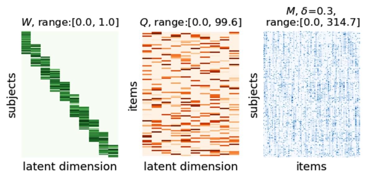
Figure 1: Synthetic $W$, $Q$ and $M$ with $\delta=0.3$.

Table 1 shows the mean error $\bar{\epsilon}$ and the standard error $s_{E}$ of the detected $k$ versus ground-truth $k^{*}=10$, across 30 generated datasets. We tested five popular detection algorithms: BCV [36], $BIC_{1}$ [53], CCC [22] and Dispersion [13]. For ICQF and $\ell_{1}$-NMF, BCV is the best detection scheme at all noise levels; $BIC_{2}$ performs well for low noise only. For the three common FA schemes, Horn’s PA [33] and MAP [57] are superior to $BIC_{2}$ [48], which aligns with empirical observations in [58, 59, 27]. ICQF with BCV outperforms $\ell_{1}$-NMF and FA at all noise levels.

Detection schemes for $k$	Noise density $\delta$
	$\delta=0.1$	$\delta=0.2$	$\delta=0.3$
ICQF (BCV)	$(0.10,0.06)$	$(0.11,0.06)$	$(0.77,0.15)$
$\ell_{1}$-NMF (BCV)	$(0.17,0.07)$	$(2.37,0.33)$	$(2.40,0.31)$
ICQF (BIC1)	(0.10, 0.06)	(0.67, 0.23)	(2.40, 0.48)
$\ell_{1}$-NMF (BIC1)	(0.90, 0.23)	(1.10, 0.30)	(2.47, 0.54)
ICQF (CCC)	(1.33, 0.24)	(1.14, 0.21)	(0.96, 0.18)
$\ell_{1}$-NMF (CCC)	NaN	NaN	NaN
ICQF (Dispersion)	(0.23, 0.09)	(0.93, 0.16)	(2.60, 0.26)
$\ell_{1}$-NMF (Dispersion)	NaN	NaN	NaN
FA-promax (PA)	$(0.17,0.07)$	$(0.53,0.10)$	$(0.87,0.14)$
FA-promax (MAP)	$(0.11,0.06)$	$(0.13,0.06)$	(1.27, 0.20)
FA-promax (BIC2)	(0.30, 0.03)	(0.93, 0.11)	NaN

Table 1: Average error and standard error ($\bar{\epsilon}$, $s_{E}$) of $k$.

4.2 Experiments with the Child Behavior Checklist (CBCL) questionnaire

4.2.1 Data

The 2001 Child Behavior Checklist (CBCL) is a general-purpose questionnaire covering different domains of psychopathology designed to screen and refer patients to pediatric psychiatry clinics, for a variety of diagnoses [31, 6, 7]. The referral is based either on raw answers on the questionnaire or syndrome-specific subscales derived from them. The checklist includes 113 questions, grouped into 8 syndrome subscales: Aggressive, Anxiety/Depressed, Attention, Rule Break, Social, Somatic, Thought, Withdrawn problems. Answers are scored on a three-point Likert scale (0=absent, 1=occurs sometimes, 2=occurs often) and the time frame for the responses is the past 6 months. We use the parent-reported CBCL responses.

The primary experiments in this paper use CBCL questionnaires from two independent studies: the Healthy Brain Network (HBN) [1] and the Adolescent Brain Cognitive Development${}^{\text{SM}}$ (ABCD) study (https://abcdstudy.org). HBN is an ongoing project to create a biobank from New York City area care-seeking children and adolescents. ABCD is a longitudinal study, starting with youths aged 9-10, to obtain a socio-demographically representative sample over time. Both datasets provide diagnostic labels for mental health conditions, of which we selected the 11 most prevalent ones (Depression, General Anxiety, ADHD, Suspected ASD, Panic, Agoraphobia, Separation and Social Anxiety, BPD, Phobia, OCD, Eating Disorder, PTSD, Sleep problems). In HBN, we use CBCL from 1335 participants, 1,001 of whom have at least one diagnosis. In ABCD, we use CBCL from 11,681 participants, 7,359 of whom have at least one diagnosis.

4.2.2 Experimental setup

Baseline methods  Our first baseline method is $\ell_{1}$- regularized NMF ($\ell_{1}$-NMF) [15], as it also imposes non-negativity and sparsity constraints. As constructs (or questions) can be correlated, we rule out other NMF methods with orthogonality constraints. FA with promax rotation (FA-promax) [32] using minimum residual as estimation method is included because it is the most commonly used technique for analyzing questionnaires and extracting latent constructs. It is also a baseline familiar to the clinical community designing questionnaires. Finally, syndrome subscales are included since they are often used for diagnostic prediction in screening. To estimate the number of factors $k$, we use BCV for $\ell_{1}$-NMF and ICQF, and Horn’s parallel analysis for FA, the best approach for each method in the synthetic questionnaire experiments in Section 4.1.

Dataset splits  Within each dataset, we first split the participants into development and held-out sets with an $80/20$ ratio. The assignment is done using stratified sampling, to keep the distribution of confounds and diagnostic labels similar across both sets. Training and validation sets are derived from the development set, as explained in each experiment. All the quantitative results are obtained on the held-out set. To increase the robustness of our analysis, and obtain measures of uncertainty, we use different seeds to resample 30 dataset splits, and carry out experiments on each split. The reported results are obtained by averaging the results on the held-out set across all 30 splits.

Model training and inference  Let $W^{\text{set}}$ denote the participant factor matrix in ICQF or NMF, or the factor score in FA, with the superscript denoting the set. Similarly, let $Q$ denote the question loadings associated with a factor in each method. Model training will yield a ($W^{\text{train}}$, $Q$) for participants in the training set. Inference with the model will produce $W^{\text{validate}}$ and $W^{\text{held-out}}$ in validation and held-out sets, using the trained $Q$ and confounds $C^{\text{validate}},C^{\text{held-out}}$ (if applicable).

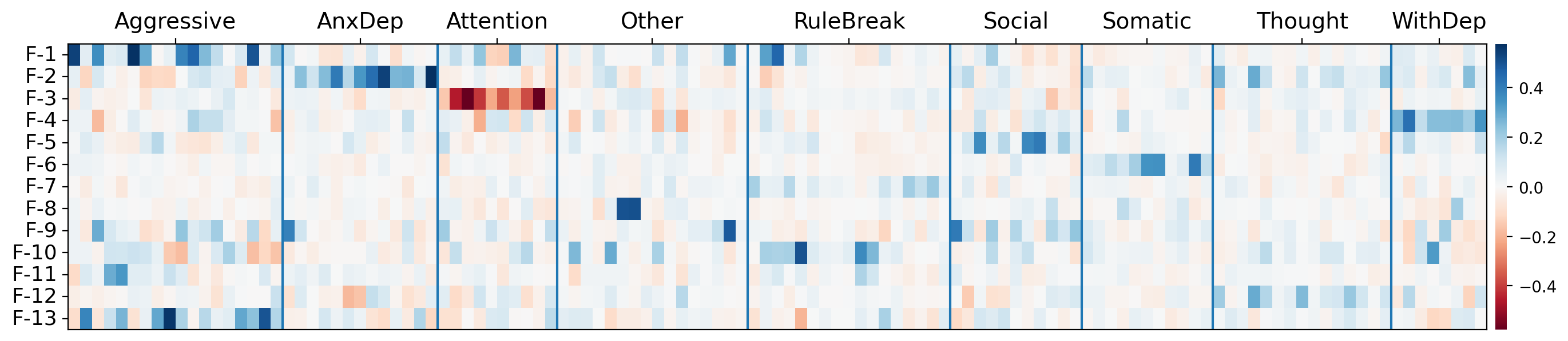
Figure 2: Heatmap of factor loadings $Q:=[{}^{R}\!Q,{}^{C}\!Q]$ from ICQF for factors proper, old/young and male/female confounds, and the implicit intercept (top) and loadings $Q$ from Factor Analysis with promax rotation (bottom). Abbreviated questions are listed at the bottom of each column. Questions are grouped by syndrome subscale; some factors are syndrome specific, while others bridge syndromes. For the enlarge version, see Appendix 6.8.

4.2.3 Experiment 1: qualitative comparison of ICQF with FA

We begin with a qualitative assessment of ICQF applied to the development set portion of the CBCL questionnaire from the HBN dataset. We estimated the latent dimensionality $k=8$ using BCV to compute an error over left-out data, at each possible $k$. The regularization parameter $\beta=0.5$ was set the same way. The top-panel of Figure 2 shows the heat map of the loading matrix $Q:=[{}^{R}\!Q,{}^{C}\!Q]$, composed of loadings ${}^{R}\!Q$ for the latent factors $W$, and the loadings ${}^{C}\!Q$ for the confounds $C$.

Given the absence of ground-truth factorizations for this questionnaire, the qualitative assessment hinges on the relation of question loadings to the syndrome subscales used in clinical practice. While there were factors that loaded primarily in questions from one subscale, as expected, we were encouraged by finding others that grouped questions from multiple subscales, in ways that were deemed sensible co-occurrences by our clinical collaborators. As a further, sanity check, we inspected the loadings of confound Old (increasing age) and observe that they covered issues such as “Argues”, “Act Young”, “Swears” and “Alcohol”. The loadings of $Q$ also reveal the relative importance among questions in each estimated factor; subscales deem all questions equally important. Visualization of each latent factor and their corresponding themes are reported in Appendix 6.9. The themes are determined by our clinical collaborators, taking into consideration the weights assigned to each factor.

For comparison, Figure 2 (bottom) shows the loadings $Q$ from Factor Analysis with promax rotation. By means of parallel analysis, we have identified a value of $k=13$, which significantly exceeds the 8 syndrome subscales that were initially established during the development of the checklist. The absence of sparsity and non-negativity control also results in a matrix that is more densely populated with both positive and negative elements, in an arbitrary range. This can present challenges when attempting to interpret the loadings in conjunction with the factor matrix $W$, also without constraints. A detailed subjective evaluation showcasing the improvement of the propsoed ICQF against FA is reported in Appendix 6.9.

4.2.4 Experiment 2: preservation of diagnostic-related information

Our first quantitative metric to compare ICQF with baseline methods is the degree to which the low-dimensional factor representation of each participant (row of $W$) retains diagnostic information, across all 11 conditions we consider. Furthermore, this metric must be evaluated as a function of training sample size. As the sample size decreases, the regularization imposed by each method becomes more influential in determining the relationship between questions.

We evaluate this by creating training sets of different sizes from the development set (80, 40, 60, and 20 % of participants, with a fixed 20% as a validation set) and factorizing each of them with ICQF and the other methods. This yields a ${W}^{\text{train}}$, ${Q}^{\text{train}}$ for each combination of method and training set size, which is then used to infer factor scores $W^{\text{held-out}}_{\%}$ from the held-out set. The same held out-set is used for every method and dataset size being compared.

To estimate diagnostic prediction performance for each ${W}^{\text{train}}$, ${Q}^{\text{train}}$ factorization, we train a separate logistic regression model with $\ell_{2}$ regularization and balanced class weights from ${W}^{\text{train}}$ for each of the 11 diagnostic labels (i.e., 11 binary classification problems). The regularization strength is fine-tuned using ${W}^{\text{validate}}$, and prediction assessment is carried out on ${W}^{\text{held-out}}$ using the receiver operating characteristic (ROC) area under the curve (AUC) metric. The use of AUC is motivated from a clinical perspective, where clinicians often apply varying thresholds for detection depending on the aim of prediction, such as screening or intervention that incurs significant costs. We repeat this procedure in both CBCL-HBN and CBCL-ABCD data.

Figure 3 shows the trend and variability (95% confidence region) of the averaged AUCs of ICQF and the baseline methods using different dataset sizes (proportions of subjects), for HBN (left) and ABCD (right). In both HBN and ABCD, the ICQF outperforms other optimal baseline methods in maintaining high AUC scores across 11 conditions, and the difference in performance increases as the sample size decreases ($p\leq 0.01$, based on a one-side Wilcoxon signed rank test and adjusted using False Discovery Rate $\alpha=0.01$), except for $\ell_{1}$-NMF at $20\%$ in CBCL-HBN). Moreover, the factorization solutions obtained with ICQF are more stable in terms of the number of dimensions $k$ ($k=8$ $\to$ 6 for ICQF, versus 8 $\to$ 3 for $\ell_{1}$-NMF and 13 $\to$ 18 for FA-promax in HBN; $k=7$ $\to$ 7 for ICQF, versus 5 $\to$ 4 for $\ell_{1}$-NMF and 20 $\to$ 17 for FA-promax in ABCD). This is particularly noteworthy in comparison to $\ell_{1}$-NMF, as it indicates the extra bounded constraints on $W$ and the approximation matrix $M_{approx}$ makes BCV detect $k$ more consistently.

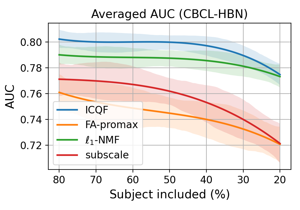
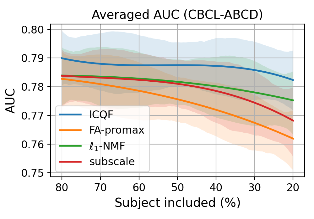
Figure 3: Trend and variability in average diagnostic prediction performance across 11 conditions, using decreasing dataset sizes, in CBCL questionnaires from HBN (left) and ABCD (right) independent datasets.

4.2.5 Experiment 3: quality of the factor loadings

Table 2: Top 2: Quality of $Q$ factor loadings at various training set sizes, within dataset. The values are the mean and standard deviation of Pearson correlation coefficients between best-matched $Q$ factors from the full dataset, and from decreasing size subsets of it. Bolded where ICQF is significantly better. Bottom: Agreement in $Q$ factor loadings between models estimated in CBCL in two independent datasets, measured in the same way.

		Factorization
Questionnaire	$n$-subjects	ICQF	FA-promax	$\ell_{1}$-NMF
CBCL-HBN	1854 (80%)	0.89 (0.07)	0.51 (0.41)	0.76 (0.18)
	1388 (60%)	0.94 (0.03)	0.62 (0.34)	0.75 (0.19)
	924 (40%)	0.92 (0.05)	0.62 (0.33)	0.75 (0.19)
	462 (20%)	0.85 (0.12)	0.54 (0.36)	0.76 (0.20)
CBCL-ABCD	7474 (80%)	0.84 (0.13)	0.43 (0.27)	0.63 (0.28)
	5604 (60%)	0.84 (0.13)	0.32 (0.30)	0.63 (0.28)
	3736 (40%)	0.77 (0.20)	0.42 (0.24)	0.63 (0.28)
	1868 (20%)	0.69 (0.25)	0.35 (0.26)	0.62 (0.29)
CBCL-HBN $\leftrightarrow$ CBCL-ABCD	full $\leftrightarrow$ full	0.75 (0.07)	0.71 (0.03)	0.68 (0.08)

Our second quantitative metric to compare ICQF with baseline methods considers the change in quality of the factor loading matrix $Q$ as training sample size decreases, to examine the effect of regularization in constraining estimates. As before, we obtain a ${W}^{\text{train}}$, ${Q}^{\text{train}}$ for each combination of method and training set size. We then compare the loading matrix each size ($Q_{\%}$) with the one obtained on the full development dataset ($Q_{\text{full}}$). We do this by greedily matching each row from $Q_{\text{full}}$ with a row from $Q_{\%}$ by their Pearson correlation, and then computing the average correlation across pairs as the score. Given that a factorization learned on a smaller dataset may have fewer factors, we do this over the first $\min(k_{\text{full}},k_{\%}$) rows only. The first two rows of Table 2 reports this score for ICQF and the two baseline factorization methods, at each dataset size, on both CBCL-HBN and CBCL-ABCD datasets. ICQF outperforms the other methods at every dataset size ($p\leq 0.01$, based on a one-side Wilcoxon signed rank test and adjusted using False Discovery Rate $\alpha=0.01$), except for $\ell_{1}$-NMF at $20\%$ in CBCL-HBN.

Our third quantitative metric is the replicability of factor loadings across independent studies (and populations). This is an important criterion for clinical research purposes, as it means that the relations between questions identified by the factorization are general. We measure this by computing $W,Q$ for the full development sets of HBN and ABCD, for ICQF and the two baseline factorization methods. For each method, we greedily match factors loadings for the HBN and ABCD factorizations, and compute the average Pearson correlation across factor pairs, reported on the third row of Table 2. We conduct similar statistical testing and observe that ICQF outperforms the other methods ($p\leq 0.05$).

5 Discussion

In this paper, we introduced ICQF, a non-negative matrix factorization method designed for questionnaire data. Our method incorporates characteristics that enhance the interpretability of the resulting factorization, as conveyed by psychiatry collaborators. We showed that their qualitative desiderata can be turned into formal constraints in the factorization problem, together with direct modelling of confounding variables, which other methods do not allow. The method is user friendly, by supporting automated estimation of the number of factors, minimizing the number of hyper-parameters, and transparently handling missing entries instead of requiring separate imputation. The characteristics above mean that ICQF required an entire optimization procedure to be derived from scratch. We provided a theoretical formalization of the problem and the procedure, and demonstrated a pair of propositions that guarantee convergence of the procedure to a local minimum and, in certain conditions, a global minimum as well.

We evaluated ICQF against alternative methods for the same purpose ($\ell_{1}$-NMF, used in the machine learning literature, and factor analysis, used in the clinical literature), on a widely used clinical questionnaire, in participants from two completely independent datasets. We designed metrics capturing the desired properties, namely preservation of diagnostic information – as this questionnaire is used for screening – and stability of solutions, at a range of dataset sizes, or across independent datasets. We carried out experiments controlling these factors, and showed that ICQF outperforms the alternative methods across the board. We have also used ICQF with 20 other questionnaires in HBN – both general-purpose and disorder-specific – in experiments not reported in this paper. Overall, results suggest that the regularization imposed by ICQF matches the underlying characteristics of questionnaire data better than other methods, in addition to promoting interpretability.

6 Supplementary Material

6.1 Optimization procedure of ICQF

Recall that the Lagrangian $\mathcal{L}_{\rho}$ of ICQF is:

$$\mathcal{L}_{\rho}(W,Q,Z,\alpha_{Z})= \frac{1}{2}\|\mathcal{M}\odot(M-Z)\|_{F}^{2}+\mathcal{I}_{\mathcal{W}}(W)+\beta\|W\|_{1,1}+\mathcal{I}_{\mathcal{Q}}(Q)$$

$$+\beta\|Q\|_{1,1}+\left\langle\alpha_{Z},Z-[W,C]Q^{T}\right\rangle$$

$$+\frac{\rho}{2}\left\|Z-[W,C]Q^{T}\right\|^{2}_{F}+\mathcal{I}_{\mathcal{Z}}(Z)$$ (12)

Following the ADMM approach, we alternatingly update primal variables $W,Q$ and the auxiliary variable $Z$, instead of updating them jointly. In particular, we iteratively solve the following sub-problems:

$$W^{(i+1)} =\underset{W\in\mathcal{W}}{\arg\min}\ \frac{\rho}{2}\left\|Z^{(i)}-[W,C]Q^{(i),T}+\frac{1}{\rho}\alpha_{Z}^{(i)}\right\|^{2}_{F}+\beta\|W\|_{1,1}$$ (Sub-problem 1)

$$Q^{(i+1)} =\underset{Q\in\mathcal{Q}}{\arg\min}\ \frac{\rho}{2}\left\|Z^{(i)}-[W^{(i+1)},C]Q^{T}+\frac{1}{\rho}\alpha_{Z}^{(i)}\right\|^{2}_{F}+\beta\|Q\|_{1,1}$$ (Sub-problem 2)

$$Z^{(i+1)} =\underset{Z\in\mathcal{Z}}{\arg\min}\ \frac{1}{2}\left\|\mathcal{M}\odot(M-Z)\right\|_{F}^{2}+\frac{\rho}{2}\left\|Z-[W^{(i+1)},C]Q^{(i+1),T}+\frac{1}{\rho}\alpha_{Z}^{(i)}\right\|^{2}_{F}$$ (Sub-problem 3)

for some penalty parameter $\rho$. We denote the Hadamard product as $\odot$. The vector of Lagrangian multipliers $\alpha_{Z}$ is updated via

$$\alpha_{Z}^{(i+1)}\leftarrow\alpha_{Z}^{(i)}+\rho(Z^{(i+1)}-[W^{(i+1)},C](Q^{(i+1)})^{T})$$ (13)

Sub-problems 1 and 2 (Equations 1 and 2)

Note that equation 1 (and similarly equation 2 by taking the transpose) can be split into row-wise constrained Lasso problem. Specifically, the $r^{\text{th}}$ row problem can be simplified into:

$$x^{*}=\underset{0\leq x_{i}\leq 1}{\arg\min}\ \frac{\rho}{2}\|b-Ax\|^{2}_{F}+\beta\|x\|_{1},\quad A=Q^{(i)},\ b=\left[Z^{(i)}-CQ^{(i),T}+\frac{1}{\rho}\alpha_{Z}^{(i)}\right]_{[r,:]}$$ (14)

Here we use the Matlab matrix notation $\bigl{[}\cdot\bigr{]}_{[r,:]}$ to represent row extraction operation. As suggested in [23] one can also use ADMM to solve equation 14:

$$x^{(i+1)} =\underset{x}{\arg\min}\ \frac{\rho}{2}\left\|b-Ax\right\|^{2}_{2}+\frac{\tau}{2}\|x-y^{(i)}+\frac{1}{\tau}\mu^{(i)}\|_{2}^{2}+\beta\|x\|_{1}$$ (15)

$$y^{(i+1)} =Proj_{[0,1]}(x^{(i+1)}+\frac{1}{\tau}\mu^{(i)})$$ (16)

$$\mu^{(i+1)} \leftarrow\mu^{(i)}+\tau(x^{(i+1)}-y^{(i+1)})$$ (17)

Similarly, $\mu$ is the vector of Lagrangian multipliers and $\tau$ is the penalty parameter. $Proj_{[0,1]}$ refers to the orthogonal projection into $[0,1]$ (inherited from the box-constraints of $W$). Equation 15 can be solved via the well-established FISTA algorithm [5]. Consider the following optimization problem

$$\arg\min_{x}\ \lambda\|x\|_{1}+\frac{1}{2}f(x)$$ (18)

The FISTA algorithm for solving 18 is summarized as follows:

Initialize: $\delta=1\mathrm{e}{-6}$; $x_{-1}=\mathbf{0},x_{0}=t_{0}=\mathbf{1}$

Input: $L$, Lipschitz constant of $\nabla f$

Result: Solution $x$ of equation 18

while $\|x_{i}-x_{i-1}\|_{2}>\delta$ do

       $\widetilde{x}_{i+1}=\operatorname*{arg\,min}_{z}\left\{\frac{\lambda}{L}\|z\|_{1}+\frac{1}{2}\left\|z-\left(x_{i}-\frac{1}{L}\nabla f(x_{i})\right)\right\|\right\}$;

       $t_{i+1}=\frac{\mathbf{1}+\sqrt{\mathbf{1}+4t_{i}^{2}}}{2}$;

       $x_{i+1}=\widetilde{x}_{i+1}+\frac{t_{i}-\mathbf{1}}{t_{i+1}}(\widetilde{x}_{i+1}-x_{i})$;

      

end while

Algorithm 1 FISTA for equation 18

To solve equation 15 with FISTA algorithm, using the notation as introduced in equation 14, we have

$$f(x)=\rho\|b-Ax\|^{2}_{2}+\tau\|x-y^{(i)}+\frac{1}{\tau}\mu^{(i)}\|^{2}_{2}$$ (19)

To compute $L$, the Lipschitz constant of $\nabla f$, we have

$$\nabla f(x) =2\rho\left(A^{T}A(x-b)+\tau(x-c)\right)$$

$$=2(\rho A^{T}A+\tau I)x-2(\rho A^{T}Ab+\tau c)$$ (20)

where $c=y^{(i)}-\frac{1}{\tau}\mu^{(i)}$. Thus, $L$ is just equal to the largest eigenvalue of $2(\rho A^{T}A+\tau I)$.

As recommended in [34], ADMM provides flexibility to use various types of loss functions and regularizations without changing the procedure. For example, we can simply change to $L_{2,1}$ norm and equation 14 becomes a constrained ridge-regression problem, which can be efficiently solved by non-negative quadratic programming algorithms. For most clinical usage, the size of questionnaire data is manageable on a single machine. However, if optimal computational and memory efficiency is required, various stochastic optimization approaches such as [42] can replace the ADMM procedure. Yet, an unbiased sampling scheme for generating random batches that handles missing responses is also needed. Such a scheme is non-trivial to obtain, especially under the multi-questionnaires scenario.

Sub-problem 3 (Equation 3)

Since both terms in equation 3 are in Frobenius-norm, $Z$ can be optimized entry-wise. In particular, we have the following closed-form solution for $Z^{(i+1)}$:

$$Z^{(i+1)}=\underset{[\min(M),\max(M)]}{Proj}\left(\mathcal{M}\odot M+\rho[W^{(i+1)},C](Q^{(i+1)})^{T}-\alpha_{Z}^{(i)}\right)\oslash(\rho\mathbbm{1}+\mathcal{M})$$ (21)

where $\mathbbm{1}$ is a 1-matrix with appropriate dimension and $\oslash$ is the Hadamard division.

6.2 Optimization procedure using coordinate descent method

The subproblems for updating $W$, $Q$ and $Z$ employ the FISTA algorithm is efficient for large dataset. However, for small or moderate data sizes, coordinate descent algorithm outperforms FISTA. In the following, we revisit the Sub-problem 2 and work out all implementation details. Recall the sub-problem 2 that updates $W$:

$$W^{(i+1)}=\arg\min_{W\in\mathcal{W}}\frac{\rho}{2}\left\|Z^{(i)}-W\left(Q^{(i)}\right)^{T}-C\left(Q_{C}^{(i)}\right)^{T}+\frac{1}{\rho}\alpha^{(i)}_{Z}\right\|^{2}_{F}+\beta_{W}\|W\|_{1,1}$$ (22)

To simplify the notation, we first divide the energy by $\frac{1}{\rho}$, followed by setting $\beta_{W}=0$. We rewrite it into a more compact expression by defining

$$V:=Z^{(i)}-C\left(Q_{C}^{(i)}\right)^{T}+\frac{1}{\rho}\alpha^{(i)}_{Z},\quad H:=\left(Q^{(i)}\right)^{T},\quad W:=W^{(i+1)}$$ (23)

Coordinate descent methods aim to conduct the following 1-variable update:

$$(W,H)\leftarrow(W+sE_{ir},H)$$ (24)

where $E_{ir}$ is a matrix same size as $W$ with all entries 0 except the $(i,r)$ element which equals 1. This update is equivalent to solve the following 1-variable optimization problem to get $s$:

$$\min_{s:0\leq W_{ir}+s\leq B_{W}}g^{W}_{ir}(s)\equiv\frac{1}{2}\left(V_{ij}-(WH)_{ij}-s\cdot H_{rj}\right)^{2}$$ (25)

Simplifying $g^{W}_{ir}(s)$, we have

$$g^{W}_{ir}(s) =\frac{1}{2}\sum_{j}\left(V_{ij}-(WH)_{ij}-sH_{rj}\right)^{2}$$

$$=g^{W}_{ir}(0)+\left(g^{W}_{ir}\right)^{\prime}(0)\cdot s+\frac{1}{2}\left(g^{W}_{ir}\right)^{\prime\prime}(0)\cdot s^{2}$$ (26)

Define

$$G^{W} :=\nabla_{W}g^{W}_{ir}(s)=WHH^{T}-VH^{T}$$ (27)

$$G^{H} :=\nabla_{H}g^{W}_{ir}(s)=W^{T}WH-W^{T}V$$ (28)

we then have

$$\left(g^{W}_{ir}\right)^{\prime}(0) =\left(G^{W}\right)_{ir}=(WHH^{T}-VH^{T})_{ir}$$ (29)

$$\left(g^{W}_{ir}\right)^{\prime\prime}(0) =\left(HH^{T}\right)_{rr}$$ (30)

and the closed form solution of $s$ is:

$$s^{*}=\min\left(\max\left(0,W_{ir}-(WHH^{T}-VH^{T})_{ir}/(HH^{T})_{rr}\right),B_{W}\right)-W_{ir}$$ (31)

Coordinate descent algorithms then update $W_{ir}$ to $W_{ir}\leftarrow W_{ir}+s^{*}$. If $\beta_{W}\neq 0$, we have,

$$W_{ir}\leftarrow\min\left(\max\left(0,W_{ir}-\left((WHH^{T}-VH^{T})_{ir}+\frac{\beta_{W}}{\rho}\right)\biggr{/}(HH^{T})_{rr}\right),B_{W}\right)$$ (32)

Notice that the update of $W$ and $H$ is invariant to the missing entries of $M$ here as $Z$ is present as a surrogate of $M$. By taking transpose, the update of $H$ can be done similarly. These update are performed in cyclic on $W$, and followed by updates on $H$ for the two sub-problems.

6.3 Details and proof of Preposition 1

In the following, we provide a self-contained convergence proof and show that, under an appropriate choice of the penalty parameter $\rho$, the ADMM optimization scheme discussed in Section 3.2 converges to a local minimum. To simplify notation, we denote $\mathbbm{V}^{(i,j,k)}=\{W^{(i)},Q^{(j)},Z^{(k)}\}$ to be the tuple of variables $W,Q$ and $Z$ during iteration $(i),(j)$ and $(k)$ respectively. If $i=j=k$, we abbreviate it as $\mathbbm{V}^{(i)}$. We also denote $R^{(i)}=[W^{(i)},C](Q^{(i)})^{T}$ and for any matrices $A,B$ with appropriate dimensions, $\langle A,B\rangle=\text{Trace}(A^{T}B)$. In the following, we are going to show that the Lagrangian is decreasing across iterations. Particularly, we consider the difference of Lagrangian between consecutive iterations:

$$\mathcal{L}_{\rho}(\mathbbm{V}^{(i+1)},\alpha_{Z}^{(i+1)})-\mathcal{L}_{\rho}(\mathbbm{V}^{(i)},\alpha_{Z}^{(i)})$$

$$= \underbrace{\mathcal{L}_{\rho}(\mathbbm{V}^{(i+1)},\alpha_{Z}^{(i+1)})-{\color[rgb]{.5,0,.5}\mathcal{L}_{\rho}(\mathbbm{V}^{(i+1)},\alpha_{Z}^{(i)})}}_{(I)}+\underbrace{{\color[rgb]{.5,0,.5}\mathcal{L}_{\rho}(\mathbbm{V}^{(i+1)},\alpha_{Z}^{(i)})}-\mathcal{L}_{\rho}(\mathbbm{V}^{(i)},\alpha_{Z}^{(i)})}_{(II)}$$ (33)

Expanding term $(I)$, we have

$$\begin{split}\mathcal{L}_{\rho}(\mathbbm{V}^{(i+1)},\alpha_{Z}^{(i+1)})-\mathcal{L}_{\rho}(\mathbbm{V}^{(i+1)},\alpha_{Z}^{(i)})&=\left\langle\alpha_{Z}^{(i+1)}-\alpha_{Z}^{(i)},Z^{(i+1)}-R^{(i+1)}\right\rangle\\ &=\frac{1}{\rho}\|\alpha_{Z}^{(i+1)}-\alpha_{Z}^{(i)}\|_{F}^{2}\end{split}$$ (34)

Expanding term $(II)$, we have

$$\mathcal{L}_{\rho}(\mathbbm{V}^{(i+1)},\alpha_{Z}^{(i)})-\mathcal{L}_{\rho}(\mathbbm{V}^{(i)},\alpha_{Z}^{(i)})$$

$$= \overbrace{\mathcal{L}_{\rho}(\mathbbm{V}^{(i+1)},\alpha_{Z}^{(i)})-{\color[rgb]{1,0,0}\mathcal{L}_{\rho}(\mathbbm{V}^{(i+1,i+1,i)},\alpha_{Z}^{(i)})}}^{(\mathcal{A})}$$

$$+\overbrace{{\color[rgb]{1,0,0}\mathcal{L}_{\rho}(\mathbbm{V}^{(i+1,i+1,i)},\alpha_{Z}^{(i)})}-{\color[rgb]{0,0,1}\mathcal{L}_{\rho}(\mathbbm{V}^{(i+1,i,i)},\alpha_{Z}^{(i)})}}^{(\mathcal{B})}$$

$$+\underbrace{{\color[rgb]{0,0,1}\mathcal{L}_{\rho}(\mathbbm{V}^{(i+1,i,i)},\alpha_{Z}^{(i)})}-L(S^{(k)},\alpha_{Z}^{(i)})}_{(\mathcal{C})}$$ (35)

Expanding ($\mathcal{A}$) by the definition, we have

$$\frac{1}{2}\|\mathcal{M}\odot(M-Z^{(i+1)})\|_{F}^{2}-\frac{1}{2}\|\mathcal{M}\odot(M-Z^{(i)})\|_{F}^{2}+\left\langle\alpha_{Z}^{(i)},Z^{(i+1)}-R^{(i+1)}\right\rangle$$

$$-\left\langle\alpha_{Z}^{(i)},Z^{(i)}-R^{(i+1)}\right\rangle+\frac{\rho}{2}\left\|Z^{(i+1)}-R^{(i+1)}\right\|^{2}_{F}-\frac{\rho}{2}\left\|Z^{(i)}-R^{(i+1)}\right\|^{2}_{F}$$

$$= \left\langle\mathcal{M}\odot(Z^{(i+1)}-M),\mathcal{M}\odot(Z^{(i+1)}-Z^{(i)})\right\rangle-\|\mathcal{M}\odot(Z^{(i+1)}-Z^{(i)})\|_{F}^{2}$$

$$+\langle\alpha^{(i)}_{Z},Z^{(i+1)}-Z^{(i)}\rangle+\rho\left\langle Z^{(i+1)}-R^{(i+1)},Z^{(i+1)}-Z^{(i)}\right\rangle-\rho\|Z^{(i+1)}-Z^{(i)}\|_{F}^{2}$$

$$= \left\langle\mathcal{M}\odot(Z^{(i+1)}-M)+\rho\cdot Z^{(i+1)}+\alpha^{(i)}_{Z}-\rho R^{(i+1)},Z^{(i+1)}-Z^{(i)}\right\rangle$$

$$-\|\mathcal{M}\odot(Z^{(i+1)}-Z^{(i)})\|_{F}^{2}-\rho\|(Z^{(i+1)}-Z^{(i)})\|_{F}^{2}$$

$$-\left\langle\mathcal{M}\odot(Z^{(i+1)}-M),(1-\mathcal{M})\odot(Z^{(i+1)}-Z^{(i)})\right\rangle$$

Since $Z^{(i+1)}$ is the minimizer of equation 3, we have

$$\left\|\mathcal{M}\odot(M-Z^{(i+1)})\right\|_{F}^{2}+\rho\left\|Z^{(i+1)}-R^{(i+1)}+\frac{1}{\rho}\alpha_{Z}^{(i)}\right\|^{2}_{F}$$

$$\leq \left\|\mathcal{M}\odot(M-Z^{(i)})\right\|_{F}^{2}+\rho\left\|Z^{(i)}-R^{(i+1)}+\frac{1}{\rho}\alpha_{Z}^{(i)}\right\|^{2}_{F}$$

which gives

$$2\left\langle\mathcal{M}\odot(Z^{(i+1)}-M),\mathcal{M}\odot(Z^{(i+1)}-Z^{(i)})\right\rangle-\|\mathcal{M}\odot(Z^{(i+1)}-Z^{(i)})\|_{F}^{2}$$

$$\leq -2\left\langle\rho\cdot Z^{(i+1)}+\alpha_{Z}^{(i)}-\rho R^{(i+1)},Z^{(i+1)}-Z^{(i)}\right\rangle+\rho\|Z^{(i+1)}-Z^{(i)}\|_{F}^{2}$$

It further implies

$$\begin{split}&\left\langle\rho\cdot Z^{(i+1)}+\alpha_{Z}^{(i)}-\rho R^{(i+1)},Z^{(i+1)}-Z^{(i)}\right\rangle\\ \leq&-\left\langle\mathcal{M}\odot(Z^{(i+1)}-M),\mathcal{M}\odot(Z^{(i+1)}-Z^{(i)})\right\rangle+\frac{1}{2}\|\mathcal{M}\odot(Z^{(i+1)}-Z^{(i)})\|_{F}^{2}\\ &+\frac{\rho}{2}\|Z^{(i+1)}-Z^{(i)}\|_{F}^{2}\end{split}$$

By direct substitution, we have

$$(\mathcal{A})$$

$$\leq \left\langle\mathcal{M}\odot(Z^{(i+1)}-M),Z^{(i+1)}-Z^{(i)}\right\rangle$$

$$-\left\langle\mathcal{M}\odot(Z^{(i+1)}-M),\mathcal{M}\odot(Z^{(i+1)}-Z^{(i)})\right\rangle$$

$$+\frac{1}{2}\|\mathcal{M}\odot(Z^{(i+1)}-Z^{(i)}\|_{F}^{2}+\frac{\rho}{2}\|Z^{(i+1)}-Z^{(i)}\|_{F}^{2}-\|\mathcal{M}\odot(Z^{(i+1)}-Z^{(i)})\|_{F}^{2}$$

$$-\rho\|(Z^{(i+1)}-Z^{(i)})\|_{F}^{2}-\left\langle\mathcal{M}\odot(Z^{(i+1)}-M),(1-\mathcal{M})\odot(Z^{(i+1)}-Z^{(i)})\right\rangle$$

$$= -\frac{1}{2}\|\mathcal{M}\odot(Z^{(i+1)}-Z^{(i)})\|_{F}^{2}-\frac{\rho}{2}\|(Z^{(i+1)}-Z^{(i)})\|_{F}^{2}\leq-\frac{\rho}{2}\|(Z^{(i+1)}-Z^{(i)})\|_{F}^{2}$$ (36)

For the second term $(\mathcal{B})$, by definition, we have,

$$(\mathcal{B})= \frac{\rho}{2}\left\|Z^{(i)}-R^{(i+1)}+\frac{1}{\rho}\alpha_{Z}^{(i)}\right\|^{2}_{F}-\frac{\rho}{2}\left\|Z^{(i)}-[W^{(i+1)},C]Q^{(i),T}+\frac{1}{\rho}\alpha_{Z}^{(i)}\right\|^{2}_{F}$$

$$+\beta\|Q^{(i+1)}\|_{1,1}-\beta\|Q^{(i)}\|_{1,1}$$

$$= \rho\left\langle R^{(i+1)}-Z^{(i)}-\frac{1}{\rho}\alpha_{Z}^{(i)},[W^{(i+1)},C](Q^{(i+1),T}-Q^{(i),T})\right\rangle$$

$$-\frac{\rho}{2}\left\|[W^{(i+1)},C](Q^{(i+1),T}-Q^{(i),T})\right\|_{F}^{2}+\beta(\|Q^{(i+1)}\|_{1,1}-\|Q^{(i)}\|_{1,1})$$

We recall that $Q$ is updated via solving constrained Lasso problems for every row $Q^{(i+1)}_{[r,:]}$:

$$y =\underset{x,0\leq x}{\arg\min}\ \beta\|x\|_{1}+\frac{\rho}{2}\|b-Ax\|^{2}_{2},$$

$$\quad\text{where}\quad A =[W^{(i+1)},C],\quad b=\left[Z^{(i)}+\frac{1}{\rho}\alpha_{Z}^{(i)}\right]_{[r,:]}$$ (37)

One obtains $y$ if and only if there exists $g\in\partial\|y\|_{1}$, the sub-differential of $\|\cdot\|_{1}$ such that

$$\rho A^{T}(Ay-b)+\beta g=\mathbf{0}.$$ (38)

As $\|\cdot\|_{1}$ is convex, we have

$$\|x\|_{1}\geq\|y\|_{1}+\left\langle x-y,g\right\rangle$$ (39)

which gives

$$\|y\|_{1}-\|x\|_{1}\leq\left\langle y-x,\frac{\rho}{\beta}A^{T}(Ay-b)\right\rangle=\left\langle A(y-x),\frac{\rho}{\beta}(Ay-b)\right\rangle$$ (40)

Re-substituting $x=Q^{(i),T}_{[r,:]}$, $y=Q^{(i+1),T}_{[r,:]}$, $A=[W^{(i+1)},C]$, $b=\left[Z^{(i)}+\frac{1}{\rho}\alpha_{Z}^{(i)}\right]_{[r,:]}$ and sum over $r$, we have

$$\beta\|Q^{(i+1)}\|_{1,1}-\beta\|Q^{(i)}\|_{1,1}$$

$$\leq -\rho\left\langle R^{(i+1)}-Z^{(i)}-\frac{1}{\rho}\alpha_{Z}^{(i)},[W^{(i+1)},C](Q^{(i+1),T}-Q^{(i),T})\right\rangle$$ (41)

Therefore, we have

$$(\mathcal{B})\leq-\frac{\rho}{2}\left\|[W^{(i+1)},C](Q^{(i+1),T}-Q^{(i),T})\right\|_{F}^{2}$$ (42)

With similar argument, we can bound $(\mathcal{C})$ by

$$(\mathcal{C})\leq-\frac{\rho}{2}\left\|[(W^{(i+1)}-W^{(i)}),C]Q^{(i),T}\right\|_{F}^{2}$$ (43)

To get an upper bound of $\|\alpha_{Z}^{(i+1)}-\alpha_{Z}^{(i)}\|_{F}^{2}$, we have

$$\|\alpha_{Z}^{(i+1)}-\alpha_{Z}^{(i)}\|_{F}^{2}$$

$$\leq \|Z^{(i+1)}-Z^{(i)}\|_{F}^{2}+\|R^{(i+1)}-R^{(i)}\|_{F}^{2}$$

$$\leq \|Z^{(i+1)}-Z^{(i)}\|_{F}^{2}+\|[W^{(i+1)},C]Q^{(i+1),T}-[W^{(i+1)},C]Q^{(i),T}\|_{F}^{2}$$

$$\ +\|[W^{(i+1)},C]Q^{(i),T}-[W^{(i)},C]Q^{(i),T}\|_{F}^{2}$$

$$\leq \|Z^{(i+1)}-Z^{(i)}\|_{F}^{2}+\|[W^{(i+1)},C](Q^{(i+1),T}-Q^{(i),T})\|_{F}^{2}$$

$$\ +\|[(W^{(i+1)}-W^{(i)}),C]Q^{(i),T}\|_{F}^{2}$$ (44)

Combining equation 34, 44, 35, 36, 42 and 43 with equation 33, we have

$$\mathcal{L}_{\rho}(\mathbbm{V}^{(i+1)},\alpha_{Z}^{(i+1)})-\mathcal{L}_{\rho}(\mathbbm{V}^{(i)},\alpha_{Z}^{(i)})$$

$$\leq \frac{1}{\rho}\left\|\alpha_{Z}^{(i+1)}-\alpha_{Z}^{(i)}\right\|_{F}^{2}-\frac{\rho}{2}\left\|Z^{(i+1)}-Z^{(i)}\right\|_{F}^{2}$$

$$-\frac{\rho}{2}\left\|[W^{(i+1)},C](Q^{(i+1),T}-Q^{(i),T})\right\|_{F}^{2}$$

$$-\frac{\rho}{2}\left\|[(W^{(i+1)}-W^{(i)}),C]Q^{(i),T}\right\|_{F}^{2}$$

$$\leq \left(\frac{1}{\rho}-\frac{\rho}{2}\right)\cdot\left(\|Z^{(i+1)}-Z^{(i)}\|_{F}^{2}+\|[W^{(i+1)},C](Q^{(i+1),T}-Q^{(i),T})\|_{F}^{2}\right.$$

$$\quad\quad\quad\quad\quad\quad+\left.\|[(W^{(i+1)}-W^{(i)}),C]Q^{(i),T}\|_{F}^{2}\right).$$ (45)

We set $\rho=3$ in all experiments for sufficiency.

6.4 Details and proof of Preposition 2

Assume that there is a ground-truth factorization $(\mathbf{W}^{*},\mathbf{Q}^{*})$ of the given $\mathbf{M}=\mathbf{W}^{*}(\mathbf{Q}^{*})^{T}$, with latent dimension $k^{*}$, where $\mathbf{W}^{*}$ and $\mathbf{Q}^{*}$ are matrix-valued random variables with entries sampled from some bounded distributions. With high probability, the error $\|\mathbf{M}-\mathbf{W}\mathbf{Q}^{T}\|_{F}^{2}$ we are minimizing is star-convex towards $(\mathbf{W}^{*},\mathbf{Q}^{*})$ whenever $k=k^{*}$ [9]. To demonstrate the importance of the choice of $k$, we consider the scenario when $k\neq k^{*}$ below.

First, a more precise assumption for ICQF is to model $\mathbf{W}$ as row-independent bounded random matrices. Recall that $W$ is generated by arranging $n$ participants’ latent representation as rows of $n\times k$ matrix, where the $n$ participants are assumed to be independent from each other and their corresponding latent representations follow a high-dimensional bounded distribution.

Second, let $(\mathbf{W}_{1},\mathbf{Q}_{1})$ and $(\mathbf{W}_{2},\mathbf{Q}_{2})$ be two factorizations with dimensions $k_{1}$ and $k_{2}$ respectively. Consider that there exists two factorizations which achieve the same critical point, i.e. (a): equivalent mismatching loss in expectation, and (b): equivalent expectation approximation to data matrix $\mathbf{M}$:

$$\textbf{(a)}:\ \mathbbm{E}\left[\|\mathbf{M}-\mathbf{W}_{1}\mathbf{Q}_{1}^{T}\|_{F}^{2}\right]=\mathbbm{E}\left[\|\mathbf{M}-\mathbf{W}_{2}\mathbf{Q}_{2}^{T}\|_{F}^{2}\right]\quad\text{and}$$

$$\textbf{(b)}:\ \mathbbm{E}[\mathbf{W}_{1}\mathbf{Q}_{1}^{T}]=\mathbbm{E}[\mathbf{W}_{2}\mathbf{Q}_{2}^{T}]$$

We also assume (c): $\mathbbm{E}\left[\sum^{n}_{j=1}(\mathbf{W}_{i})_{j\kappa}^{2}\right]:=\sigma_{\mathbf{W}_{i}}^{2}$ and $\mathbbm{E}\left[\sum^{m}_{j=1}(\mathbf{Q}_{i})_{j\kappa}^{2}\right]:=\sigma_{\mathbf{Q}_{i}}^{2}$ for all $\kappa=k_{i}$, $i=1,2$.

Expanding (a), we have

$$\mathbbm{E}\left[\text{Trace}\left((\mathbf{M}-\mathbf{W}_{1}\mathbf{Q}_{1}^{T})^{T}(\mathbf{M}-\mathbf{W}_{1}\mathbf{Q}_{1}^{T})\right)\right]$$

$$= \mathbbm{E}\left[\text{Trace}\left((\mathbf{M}-\mathbf{W}_{2}\mathbf{Q}_{2}^{T})^{T}(\mathbf{M}-\mathbf{W}_{2}\mathbf{Q}_{2}^{T})\right)\right]$$

This gives

$$\mathbbm{E}\left[\text{Trace}\left(\mathbf{W}_{1}^{T}\mathbf{W}_{1}\mathbf{Q}_{1}^{T}\mathbf{Q}_{1}-2\mathbf{M}^{T}\mathbf{W}_{1}\mathbf{Q}_{1}^{T}\right)\right]$$

$$= \mathbbm{E}\left[\text{Trace}\left(\mathbf{W}_{2}^{T}\mathbf{W}_{2}\mathbf{Q}_{2}^{T}\mathbf{Q}_{2}-2\mathbf{M}^{T}\mathbf{W}_{2}\mathbf{Q}_{2}^{T}\right)\right]$$

Denote $\mathbbm{E}[\mathbf{W}_{i}]=\mu_{\mathbf{W}_{i}}$, $\mathbbm{E}[\mathbf{Q}_{i}]=\mu_{\mathbf{Q}_{i}}$ for $i=1,2$, we have $\mathbf{W}_{i}=\bar{\mathbf{W}}_{i}+\mu_{\mathbf{W}_{i}}$ and $\mathbf{Q}_{i}=\bar{\mathbf{Q}}_{i}+\mu_{\mathbf{Q}_{i}}$, where $\bar{\mathbf{W}}_{i}$ and $\bar{\mathbf{Q}}_{i}$ denote the corresponding centered variables. Note that by the independence of $\mathbf{W}_{i}$ and $\mathbf{Q}_{i}$ and linearity of trace and expectation operator,

$$\mathbbm{E}\left[\text{Trace}\left(\mathbf{M}^{T}\mathbf{W}_{1}\mathbf{Q}_{1}^{T}\right)\right]$$

$$= \mathbbm{E}\left[\text{Trace}\left(\mathbf{M}^{T}\bar{\mathbf{W}}_{1}\bar{\mathbf{Q}}_{1}^{T}+\mathbf{M}^{T}\bar{\mathbf{W}}_{1}\mu_{\mathbf{Q}_{1}}^{T}+\mathbf{M}^{T}\mu_{\mathbf{W}_{1}}\bar{\mathbf{Q}}_{1}^{T}+\mathbf{M}^{T}\mu_{\mathbf{W}_{1}}\mu_{\mathbf{Q}_{1}}^{T}\right)\right]$$

$$= \text{Trace}(\mathbf{M}^{T}\mathbbm{E}[\mathbf{W}_{1}]\mathbbm{E}[\mathbf{Q}_{1}^{T}])$$

$$= \text{Trace}(\mathbf{M}^{T}\mathbbm{E}[\mathbf{W}_{2}]\mathbbm{E}[\mathbf{Q}_{2}^{T}])$$

$$= \mathbbm{E}\left[\text{Trace}\left(\mathbf{M}^{T}\mathbf{W}_{2}\mathbf{Q}_{2}^{T}\right)\right]$$ (46)

which yields

$$\mathbbm{E}\left[\text{Trace}\left(\mathbf{W}_{1}^{T}\mathbf{W}_{1}\mathbf{Q}_{1}^{T}\mathbf{Q}_{1}\right)\right]=\mathbbm{E}\left[\text{Trace}\left(\mathbf{W}_{2}^{T}\mathbf{W}_{2}\mathbf{Q}_{2}^{T}\mathbf{Q}_{2}\right)\right]$$ (47)

Consider $\mathbbm{E}\left[\text{Trace}\left(\mathbf{W}_{1}^{T}\mathbf{W}_{1}\mathbf{Q}_{1}^{T}\mathbf{Q}_{1}\right)\right]$ via definition, we have

$$\mathbbm{E}\left[\text{Trace}\left(\mathbf{W}_{1}^{T}\mathbf{W}_{1}\mathbf{Q}_{1}^{T}\mathbf{Q}_{1}\right)\right]$$

$$= \text{Trace}\left(\mathbbm{E}\left[\mathbf{W}_{1}^{T}\mathbf{W}_{1}\right]\mathbbm{E}\left[\mathbf{Q}_{1}^{T}\mathbf{Q}_{1}\right]\right)$$

$$= \text{Trace}\left(\mathbbm{E}\begin{bmatrix}\left(\sum^{n}_{j=1}(\mathbf{W}_{1})_{j1}^{2}\right)&&\ast\\ &\ddots&\\ \ast&&\left(\sum^{n}_{j=1}(\mathbf{W}_{1})_{jk_{1}}^{2}\right)\end{bmatrix}\right.$$

$$\quad\quad\quad\quad\quad\quad\times\left.\mathbbm{E}\begin{bmatrix}\left(\sum^{m}_{j=1}(\mathbf{Q}_{1})_{j1}^{2}\right)&&0\\ &\ddots&\\ 0&&\left(\sum^{m}_{j=1}(\mathbf{Q}_{1})_{jk_{1}}^{2}\right)\end{bmatrix}\right)$$

$$= \sum_{\kappa=1}^{k_{1}}\mathbbm{E}\left[\sum^{n}_{j=1}(\mathbf{W}_{1})_{j\kappa}^{2}\right]\mathbbm{E}\left[\sum^{m}_{j=1}(\mathbf{Q}_{1})_{j\kappa}^{2}\right]$$ (48)

Incorporating assumption (c), we have

$$\mathbbm{E}\left[\text{Trace}\left(\mathbf{W}_{1}^{T}\mathbf{W}_{1}\mathbf{Q}_{1}^{T}\mathbf{Q}_{1}\right)\right]=k_{1}\sigma_{\mathbf{W}_{1}}^{2}\sigma_{\mathbf{Q}_{1}}^{2}$$ (49)

Consider equation 47 with $k_{2}>k_{1}$. For $\mathbf{W}_{1},\mathbf{Q}_{1}$, W.L.O.G. we pad $k_{2}-k_{1}$ columns of zeros. Moreover, let $\mathbf{P}$ be an optimal $k_{2}\times k_{2}$ permutation matrix, we also have

$$\mathbbm{E}\left[\text{Trace}\left((\mathbf{W}_{2}\mathbf{P})^{T}\mathbf{W}_{2}\mathbf{P}(\mathbf{Q}_{2}\mathbf{P})^{T}\mathbf{Q}_{2}\mathbf{P}\right)\right] =\mathbbm{E}\left[\text{Trace}\left(\mathbf{W}_{2}^{T}\mathbf{W}_{2}\mathbf{Q}_{2}^{T}\mathbf{Q}_{2}\right)\right]$$

$$=k_{2}\sigma_{\mathbf{W}_{2}}^{2}\sigma_{\mathbf{Q}_{2}}^{2}$$ (50)

Combining with equation 47, it is equivalent to

$$k_{1}\sigma_{\mathbf{W}_{1}}^{2}\sigma_{\mathbf{Q}_{1}}^{2}=k_{2}\sigma_{\mathbf{W}_{2}}^{2}\sigma_{\mathbf{Q}_{2}}^{2}$$ (51)

which gives

$$\mathbb{E}\left[\|\mathbf{W}_{1}\|_{F}^{2}\right]=\frac{\sigma_{\mathbf{Q}_{2}}^{2}}{\sigma_{\mathbf{Q}_{1}}^{2}}\mathbb{E}\left[\|\mathbf{W}_{2}\|_{F}^{2}\right]=\frac{\sigma_{\mathbf{Q}_{2}}^{2}}{\sigma_{\mathbf{Q}_{1}}^{2}}\mathbb{E}\left[\|\mathbf{W}_{2}\mathbf{P}\|_{F}^{2}\right]$$ (52)

To evaluate the impact of interpretability of latent representation under different latent dimension, we consider $\mathbbm{E}\left[\|\mathbf{W}_{1}-\mathbf{W}_{2}\mathbf{P}\|_{F}^{2}\right]$:

$$\mathbbm{E}\left[\|\mathbf{W}_{1}-\mathbf{W}_{2}\mathbf{P}\|_{F}^{2}\right] =\mathbbm{E}\left[\text{Trace}\left((\mathbf{W}_{1}-\mathbf{W}_{2}\mathbf{P})^{T}(\mathbf{W}_{1}-\mathbf{W}_{2}\mathbf{P})\right)\right]$$

$$=\mathbbm{E}\left[\|\mathbf{W}_{1}\|_{F}^{2}\right]+\frac{\sigma_{\mathbf{Q}_{1}}^{2}}{\sigma_{\mathbf{Q}_{2}}^{2}}\mathbbm{E}\left[\|\mathbf{W}_{1}\|_{F}^{2}\right]-2\mathbbm{E}\left[\text{Trace}(\mathbf{W}_{1}^{T}\mathbf{W}_{2}\mathbf{P})\right]$$ (53)

As $\text{Trace}(\mathbf{W}_{1}^{T}\mathbf{W}_{2}P)\leq\|\mathbf{W}_{1}\|_{F}\|\mathbf{W}_{2}\mathbf{P}\|_{F}$, we also have

$$\mathbbm{E}\left[\text{Trace}(\mathbf{W}_{1}^{T}\mathbf{W}_{2}\mathbf{P})\right] \leq\mathbbm{E}\left[\|\mathbf{W}_{1}\|_{F}\right]\cdot\mathbbm{E}\left[\|\mathbf{W}_{2}\mathbf{P}\|_{F}\right]$$

$$\leq\sqrt{\mathbbm{E}\left[\|\mathbf{W}_{1}\|_{F}^{2}\right]\cdot\mathbbm{E}\left[\|\mathbf{W}_{2}\|_{F}^{2}\right]}=\sqrt{\frac{\sigma_{\mathbf{Q}_{1}}^{2}}{\sigma_{\mathbf{Q}_{2}}^{2}}}\mathbbm{E}\left[\|\mathbf{W}_{1}\|_{F}^{2}\right]$$ (54)

which implies

$$\mathbbm{E}\left[\|\mathbf{W}_{1}-\mathbf{W}_{2}\mathbf{P}\|_{F}^{2}\right] \geq\left(1-2\sqrt{\frac{\sigma_{\mathbf{Q}_{1}}^{2}}{\sigma_{\mathbf{Q}_{2}}^{2}}}+\frac{\sigma_{\mathbf{Q}_{1}}^{2}}{\sigma_{\mathbf{Q}_{2}}^{2}}\right)\mathbbm{E}\left[\|\mathbf{W}_{1}\|_{F}^{2}\right]$$

$$=\left(1-\sqrt{\frac{\sigma_{\mathbf{Q}_{1}}^{2}}{\sigma_{\mathbf{Q}_{2}}^{2}}}\right)^{2}\mathbbm{E}\left[\|\mathbf{W}_{1}\|_{F}^{2}\right]$$ (55)

Since $\mathbf{W}_{i}$ is generated from row-wise independent bounded distribution, if we add a mild assumption that $\sigma_{\mathbf{W}_{i}}^{2}:=\sigma_{\mathbf{W}}^{2}$ for all $i$ through re-scaling, Equation 51 implies $k_{1}\sigma_{\mathbf{Q}_{1}}^{2}=k_{2}\sigma_{\mathbf{Q}_{2}}^{2}$ and therefore

$$\mathbbm{E}\left[\|\mathbf{W}_{1}-\mathbf{W}_{2}\|_{F}^{2}\right] \geq\left(1-2\sqrt{\frac{k_{2}}{k_{1}}}+\frac{k_{2}}{k_{1}}\right)\mathbbm{E}\left[\|\mathbf{W}_{1}\|_{F}^{2}\right]$$

$$=\left(\sqrt{\frac{k_{2}}{k_{1}}}-1\right)^{2}\mathbbm{E}\left[\|\mathbf{W}_{1}\|_{F}^{2}\right]$$ (56)

If we substitute $k_{1}=k^{*}$, $(\mathbf{W}_{1},\mathbf{Q}_{1})=(\mathbf{W}^{*},\mathbf{Q}^{*})$, we have

$$\mathbbm{E}\left[\|\mathbf{W}^{*}-\mathbf{W}_{2}\|_{F}^{2}\right]\geq\left(\sqrt{\frac{k_{2}}{k^{*}}}-1\right)^{2}\mathbbm{E}\left[\|\mathbf{W}^{*}\|_{F}^{2}\right]$$ (57)

which means the relative expected difference between $\mathbf{W}^{*}$ and $\mathbf{W}_{2}$ is bounded below by $\left(\sqrt{\frac{k_{2}}{k^{*}}}-1\right)^{2}$.

To prove that equation 57 holds in general, we consider the matrix concentration inequalities and show that large deviations from their means are exponentially unlikely. Benefitting from the model constraints, we can further assume that $W$ is generated from some high dimensional bounded distribution. In the following, we make use of the main theorem proposed in [43] on concentration of non-commutative random matrices polynomials. As $\mathbf{W}_{i}$ are generated from bounded distributions, $\|\mathbf{W}_{i}-\mathbbm{E}[\mathbf{W}_{i}]\|_{F}$ is uniformly bounded. Therefore, it satisfies the convex concentration properties. The theorem achieves the following results:

$$\mathbbm{P}\left\{\|\mathbf{W}\|_{F}^{2}-\mathbbm{E}\left[\|\mathbf{W}\|_{F}^{2}\right]>tkn^{2}\right\}\leq C_{1}\exp\left(-C_{2}\min(t^{2},t^{1/2})n\right)$$ (58)

Recall that

$$\mathbbm{E}\left[\|\mathbf{W}_{1}-\mathbf{W}_{2}P\|_{F}^{2}\right]=\mathbbm{E}\left[\|\mathbf{W}_{1}\|_{F}^{2}\right]+\frac{\sigma_{\mathbf{Q}_{1}}^{2}}{\sigma_{\mathbf{Q}_{2}}^{2}}\mathbbm{E}\left[\|\mathbf{W}_{1}\|_{F}^{2}\right]-2\mathbbm{E}\left[\text{Trace}(\mathbf{W}_{1}^{T}\mathbf{W}_{2}\mathbf{P})\right]$$

. By padding $\mathbf{W}_{1}$ and $\mathbf{W}_{2}$ with zeros columns, we assume that $\mathbf{W}_{i}$ are all $n\times n$ matrices. Then the probability that the any one of the terms is deviating from their mean by a relative factor $\epsilon$ is less than $C_{1}\exp(-C_{2}\epsilon^{2}n)$ for some small $\epsilon$. By the union bound, the probability that the either of them does is less than or equal to $C_{3}\exp(-C_{4}\epsilon^{2}n)$.

6.5 Visualization of the experimental setup for diagnostic prediction evaluation

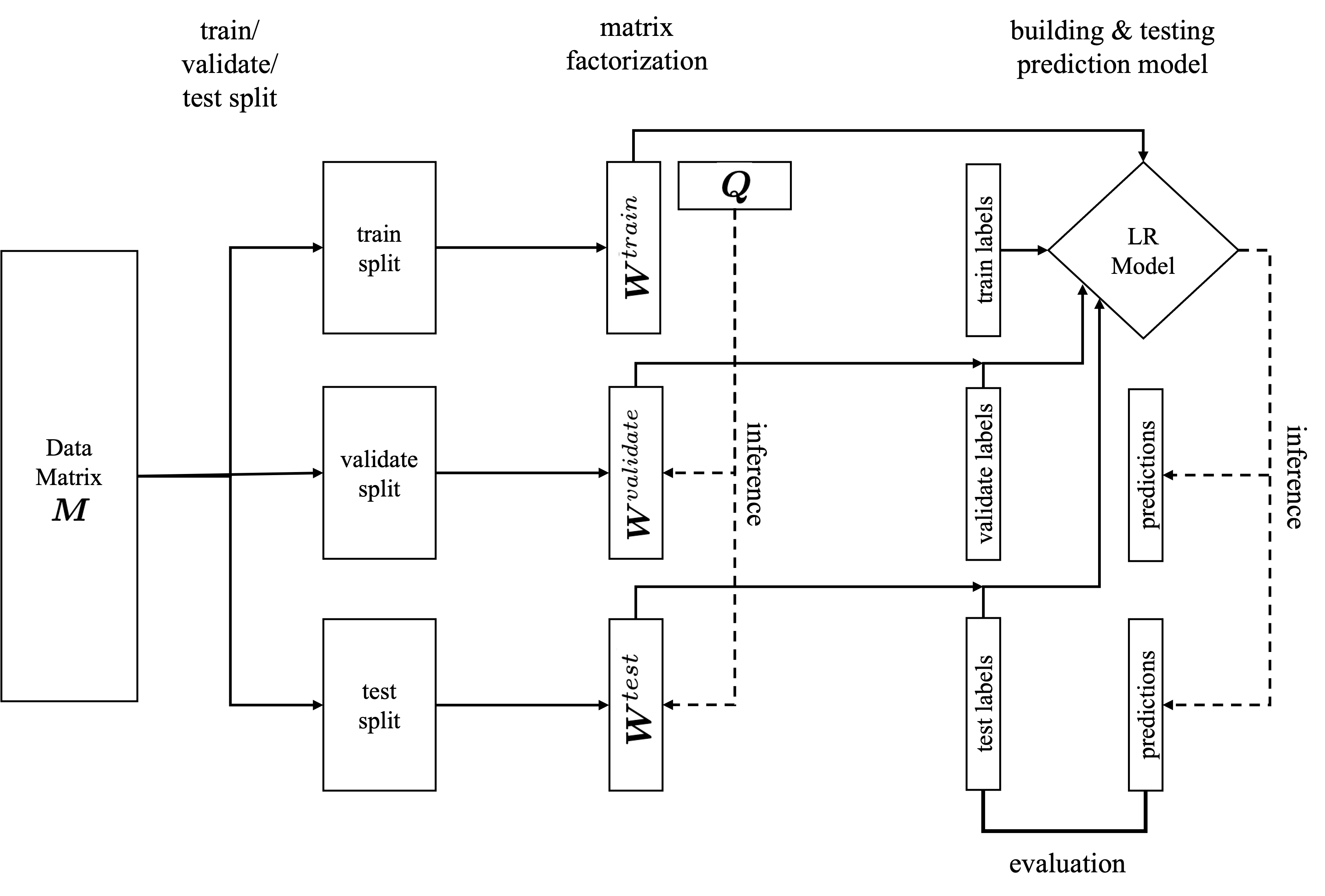
Figure 4: Setup for diagnostic prediction experiments.

6.6 Table of the 21 questionnaires used in HBN dataset

Table 3: Optimal $(k,\beta)$ of all 21 questionnaires.

Questionnaire	Abbreviation	$n$ questions	Subscales	$k$	$\beta$
Affective Reactivity Index (Parent-Report)	ARI_P	7	nan	2	0.01
Affective Reactivity Index (Self-Report)	ARI_S	7	nan	2	0.01
Autism Spectrum Screening Questionnaire	ASSQ	27	nan	2	0.01
Conners 3 (Self-Report)	C3SR	9		4	0.05
Child Behavior Checklist	CBCL	119	9	8	0.5
Extended Strengths and Weaknesses Assessment of Normal Behavior	ESWAN	65	nan	13	0.2
Inventory of Callous-Unemotional Traits (Parent-Report)	ICU_P	24	3	4	0.1
Inventory of Callous-Unemotional Traits (Self-Report)	ICU_SR	24	3	3	0.1
Mood and Feelings Questionnaire (Parent-Report)	MFQ_P	34	nan	2	0.1
Mood and Feelings Questionnaire (Self-Report)	MFQ_SR	33	nan	2	0.1
The Positive and Negative Affect Schedule	PANAS	20	2	2	0.05
Repetitive Behaviors Scale	RBS	43	5	3	0.1
Screen for Child Anxiety Related Disorders (Parent-Report)	SCARED_P	41	5	3	0.1
Screen for Child Anxiety Related Disorders (Self-Report)	SCARED_SR	41	5	3	0.3
Social Communication Questionnaire	SCQ	40	nan	4	0.02
Strength and Difficulties Questionnaire	SDQ	33	9	6	0.05
Social Responsiveness Scale (School Age)	SRS	65	7	3	0.5
The Strengths and Weaknesses Assessment of Normal Behavior Rating Scale for ADHD	SWAN	18	2	3	0.02
Symptom Checklist (Parent-Report)	SympChck	63	nan	3	0.1
Teacher Report Form (School Age)	TRF	116	19	8	0.5
Youth Self Report	YSR	119	11	3	0.2

6.7 Synthetic example and the factorization results

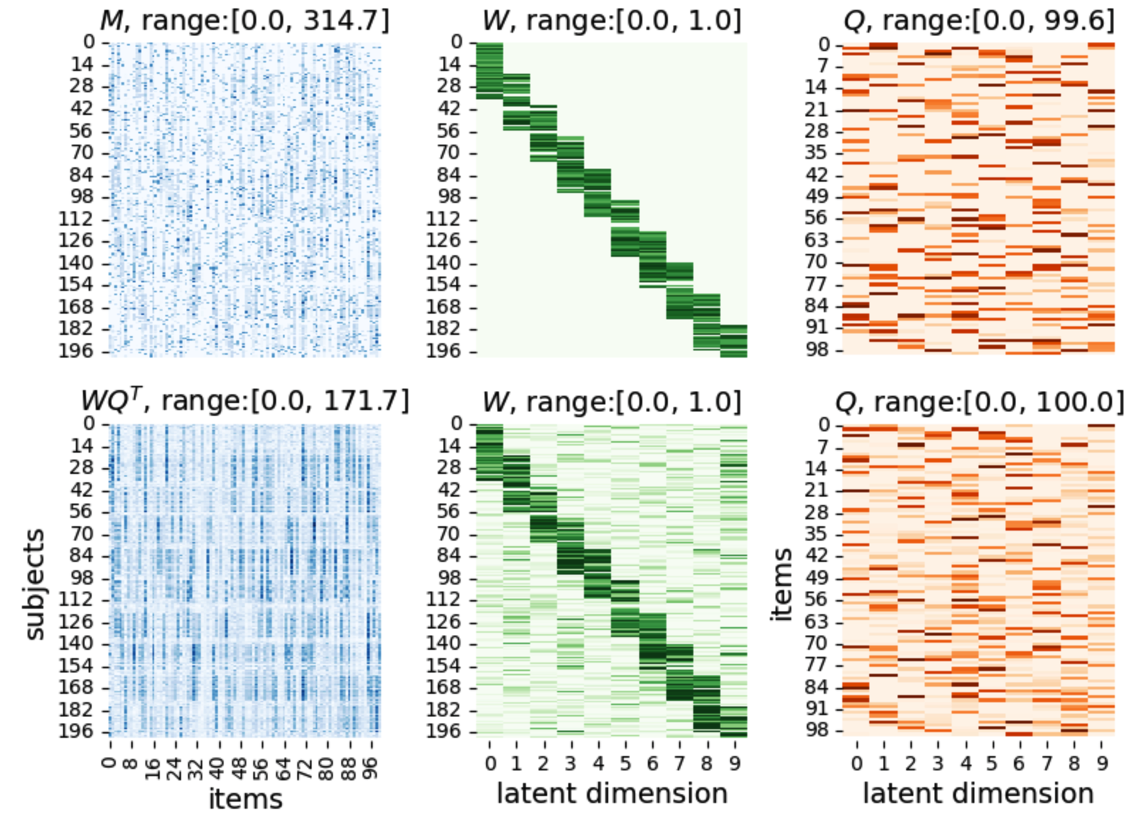
Figure 5: Top row: (left) The synthetic noisy data matrix $M$; (center): The ground-truth $W$; (right): The groud-truth $Q$. Bottom row: (left) Reconstructed $M=WQ^{T}$ based on the estimated $W$ and $Q$; (center): The estimated $W$ by ICQF; (right): The estimated $Q$ by ICQF.

6.8 Question embedding ($Q$) obtained from the Factor analysis, and the proposed method with optimal latent dimension.

6.9 Visualization and subjective evaluation of question embedding $Q$ in CBCL-HBN questionnaire

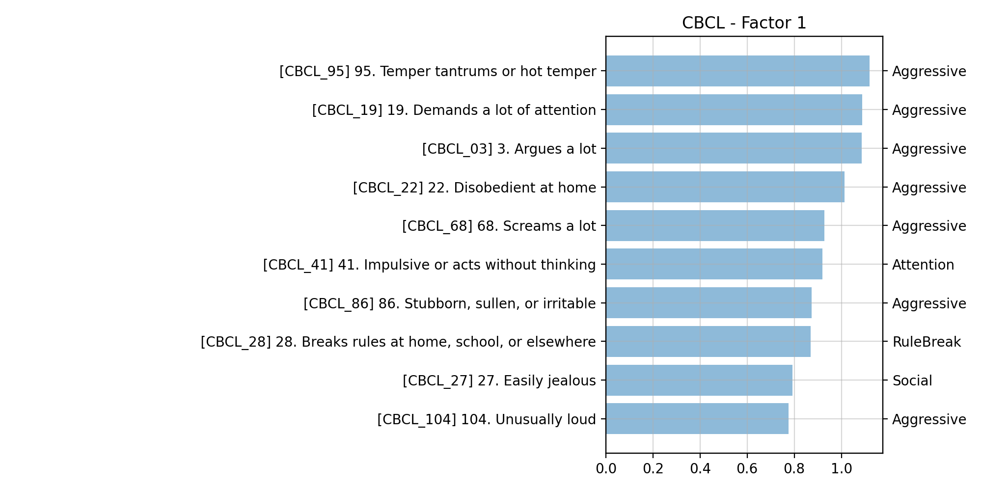
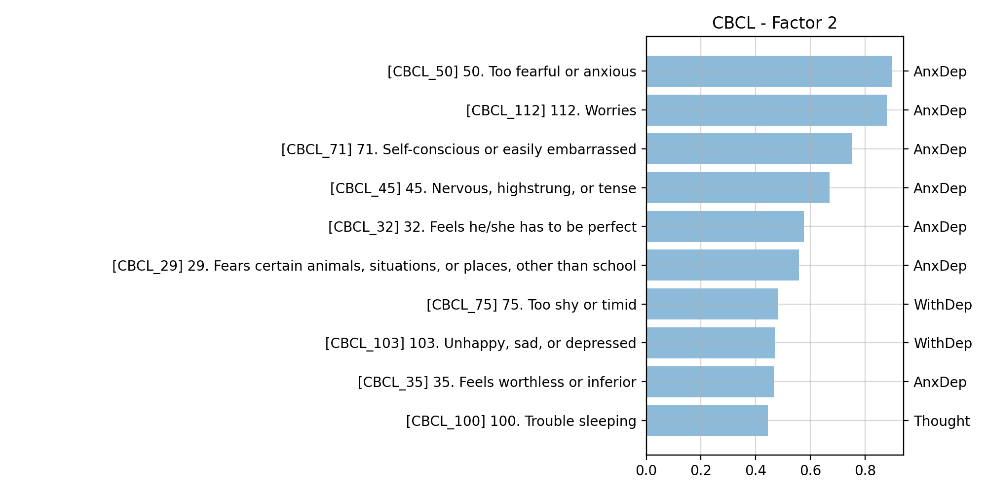
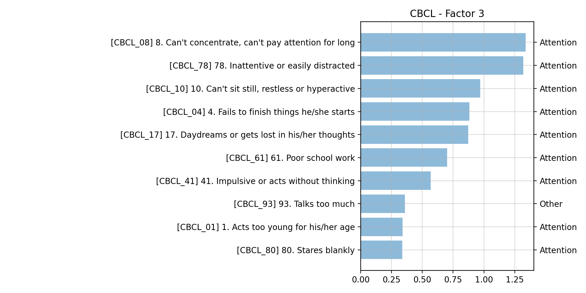
Figure 6: Top 10 questions ranked by $Q$ in CBCL using $Q$ obtained from ICQF (Factor 1-3).

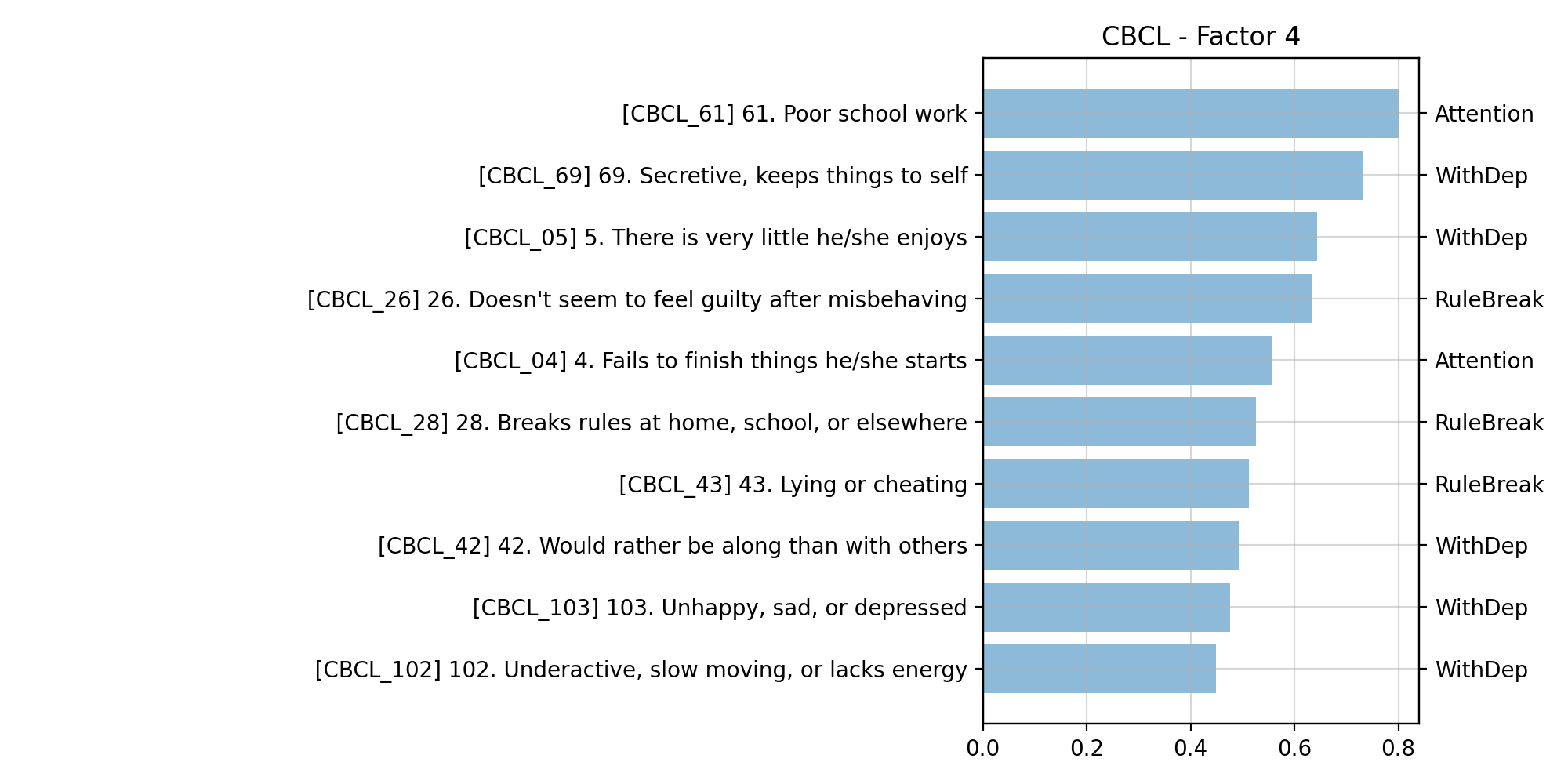
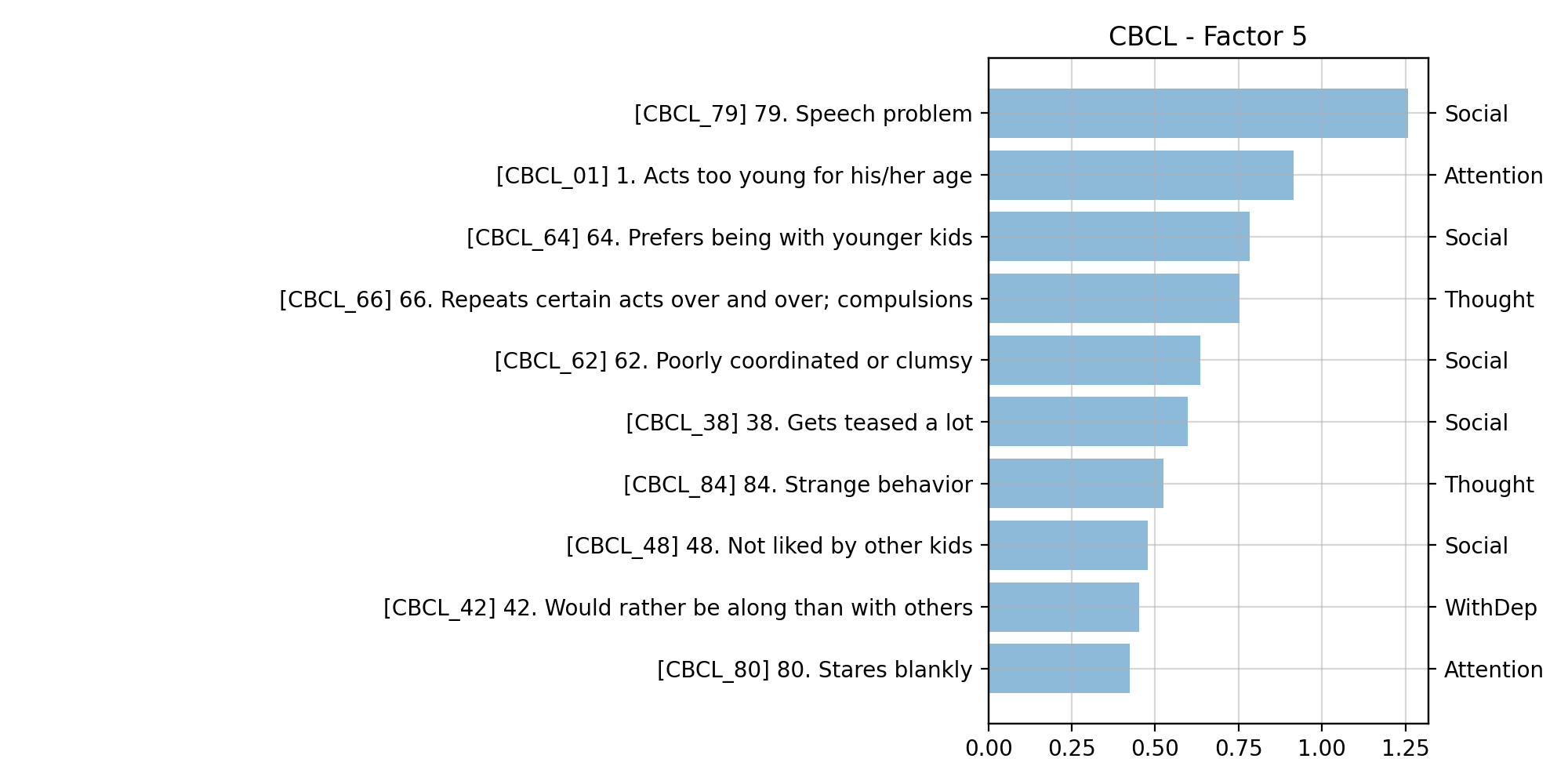
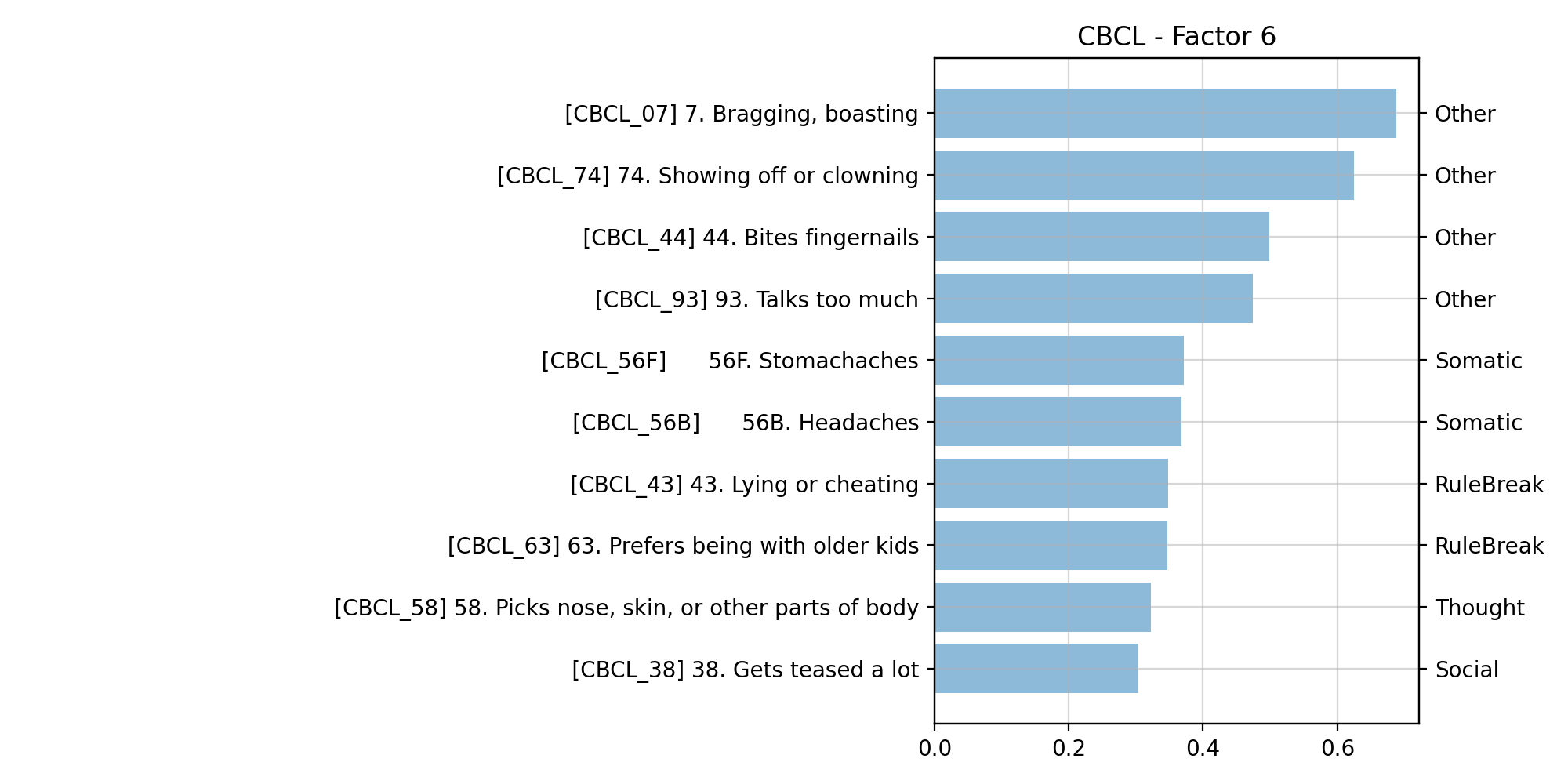
Figure 7: Top 10 questions ranked by $Q$ in CBCL using $Q$ obtained from ICQF (Factor 4-6).

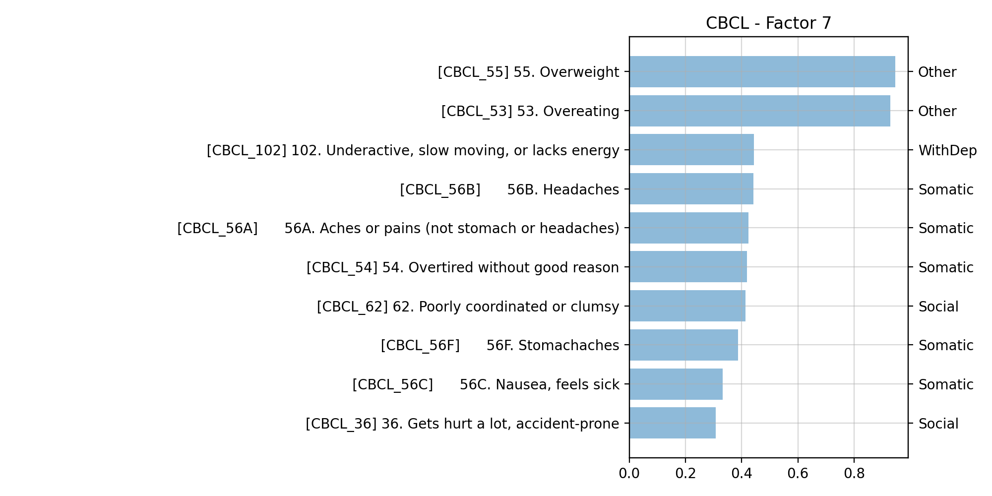
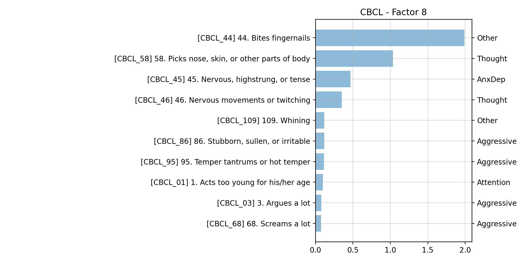
Figure 8: Top 10 questions ranked by $Q$ in CBCL using $Q$ obtained from ICQF (Factor 7-8).

Factor	Theme
CBCL Factor-1	irritability and oppositionality
CBCL Factor-2	anxiety
CBCL Factor-3	inattention and hyperactivity
CBCL Factor-4	cognitive problems, disociality and callousness
CBCL Factor-5	cognitive + fine motor problems
CBCL Factor-6	body-focused repetitive behaviors
CBCL Factor-7	somatic problems
CBCL Factor-8	body-focused repetitive behaviors

Table 4: Themes assigned to each CBCL factor by domain experts, summarizing the corresponding latent factors based on their components.

We also carried out subjective evaluations of the factor loadings produced by our method and factor analysis. Our clinical collaborators observed that:

• ICQF groups questions that are strongly related to cognitive impairments (which increase risk for psychopathology) into a separate factor (F5) whereas these are distributed across multiple factors in FA

• ICQF recovers the well-known dual comorbidly of depressive features with both anxiety symptoms (F2) and externalizing symptoms (F4) , whereas these dual links are missed by FA which puts most WithDep items into one factor with little other loadings (F4)

• ICQF groups distinctive body-focused repetitive behaviors into a distinct factor (F8) whereas these are not well differentiated by FA

• ICQF concentrates questions related to proactive aggression and antisociality into a single factor (F1) with captures the closely related feature of impulsivity. In contrast, FA distributes questions related to aggression into two factors (F1 and F13) which are weakly differentiated with regard to their loadings for other questions.

References

- [1] Alexander, L.M., Escalera, J., Ai, L., Andreotti, C., Febre, K., Mangone, A., Vega-Potler, N., Langer, N., Alexander, A., Kovacs, M., et al.: An open resource for transdiagnostic research in pediatric mental health and learning disorders. Scientific data 4(1), 1–26 (2017)
- [2] Arora, S., Cohen, N., Hu, W., Luo, Y.: Implicit regularization in deep matrix factorization. Advances in Neural Information Processing Systems 32 (2019)
- [3] Bandalos, D.L., Boehm-Kaufman, M.R.: Four common misconceptions in exploratory factor analysis. In: Statistical and methodological myths and urban legends, pp. 81–108. Routledge (2010)
- [4] Bartlett, M.S.: Tests of significance in factor analysis. British journal of psychology (1950)
- [5] Beck, A., Teboulle, M.: A fast iterative shrinkage-thresholding algorithm for linear inverse problems. SIAM journal on imaging sciences 2(1), 183–202 (2009)
- [6] Biederman, J., Monuteaux, M., Kendrick, E., Klein, K., Faraone, S.: The cbcl as a screen for psychiatric comorbidity in paediatric patients with adhd. Archives of Disease in Childhood 90(10), 1010–1015 (2005)
- [7] Biederman, J., DiSalvo, M., Vaudreuil, C., Wozniak, J., Uchida, M., Woodworth, K.Y., Green, A., Faraone, S.V.: Can the child behavior checklist (cbcl) help characterize the types of psychopathologic conditions driving child psychiatry referrals? Scandinavian journal of child and adolescent psychiatry and psychology (2020)
- [8] Bishop, C.M., Nasrabadi, N.M.: Pattern recognition and machine learning, vol. 4. Springer (2006)
- [9] Bjorck, J., Kabra, A., Weinberger, K.Q., Gomes, C.: Characterizing the loss landscape in non-negative matrix factorization. In: Proceedings of the AAAI Conference on Artificial Intelligence. vol. 35, pp. 6768–6776 (2021)
- [10] Boutsidis, C., Gallopoulos, E.: Svd based initialization: A head start for nonnegative matrix factorization. Pattern recognition 41(4), 1350–1362 (2008)
- [11] Boyd, S., Parikh, N., Chu, E., Peleato, B., Eckstein, J., et al.: Distributed optimization and statistical learning via the alternating direction method of multipliers. Foundations and Trends® in Machine learning 3(1), 1–122 (2011)
- [12] Browne, M.W.: An overview of analytic rotation in exploratory factor analysis. Multivariate behavioral research 36(1), 111–150 (2001)
- [13] Brunet, J.P., Tamayo, P., Golub, T.R., Mesirov, J.P.: Metagenes and molecular pattern discovery using matrix factorization. Proceedings of the national academy of sciences 101(12), 4164–4169 (2004)
- [14] Choi, S.: Algorithms for orthogonal nonnegative matrix factorization. In: 2008 ieee international joint conference on neural networks (ieee world congress on computational intelligence). pp. 1828–1832. IEEE (2008)
- [15] Cichocki, A., Phan, A.H.: Fast local algorithms for large scale nonnegative matrix and tensor factorizations. IEICE transactions on fundamentals of electronics, communications and computer sciences 92(3), 708–721 (2009)
- [16] Ding, C., Li, T., Peng, W., Park, H.: Orthogonal nonnegative matrix t-factorizations for clustering. In: Proceedings of the 12th ACM SIGKDD international conference on Knowledge discovery and data mining. pp. 126–135 (2006)
- [17] Ding, C.H., Li, T., Jordan, M.I.: Convex and semi-nonnegative matrix factorizations. IEEE transactions on pattern analysis and machine intelligence 32(1), 45–55 (2008)
- [18] Ding, G., Guo, Y., Zhou, J.: Collective matrix factorization hashing for multimodal data. In: Proceedings of the IEEE conference on computer vision and pattern recognition. pp. 2075–2082 (2014)
- [19] Eggert, J., Korner, E.: Sparse coding and nmf. In: 2004 IEEE International Joint Conference on Neural Networks (IEEE Cat. No. 04CH37541). vol. 4, pp. 2529–2533. IEEE (2004)
- [20] Fan, J.: Multi-mode deep matrix and tensor factorization. In: International Conference on Learning Representations (2021)
- [21] Fan, J., Cheng, J.: Matrix completion by deep matrix factorization. Neural Networks 98, 34–41 (2018)
- [22] Fogel, P., Young, S.S., Hawkins, D.M., Ledirac, N.: Inferential, robust non-negative matrix factorization analysis of microarray data. Bioinformatics 23(1), 44–49 (2007)
- [23] Gaines, B.R., Kim, J., Zhou, H.: Algorithms for fitting the constrained lasso. Journal of Computational and Graphical Statistics 27(4), 861–871 (2018)
- [24] Gaskin, C.J., Happell, B.: On exploratory factor analysis: A review of recent evidence, an assessment of current practice, and recommendations for future use. International journal of nursing studies 51(3), 511–521 (2014)
- [25] Gaynanova, I., Li, G.: Structural learning and integrative decomposition of multi-view data. Biometrics 75(4), 1121–1132 (2019)
- [26] Golub, G.H., Van Loan, C.F.: Matrix computations. JHU press (2013)
- [27] Goretzko, D., Pham, T.T.H., Bühner, M.: Exploratory factor analysis: Current use, methodological developments and recommendations for good practice. Current Psychology 40(7), 3510–3521 (2021)
- [28] Gorsuch, R.L.: Factor analysis: Classic edition. Routledge (2014)
- [29] Gunasekar, S., Yamada, M., Yin, D., Chang, Y.: Consistent collective matrix completion under joint low rank structure. In: Artificial Intelligence and Statistics. pp. 306–314. PMLR (2015)
- [30] Hayton, J.C., Allen, D.G., Scarpello, V.: Factor retention decisions in exploratory factor analysis: A tutorial on parallel analysis. Organizational research methods 7(2), 191–205 (2004)
- [31] Heflinger, C.A., Simpkins, C.G., Combs-Orme, T.: Using the cbcl to determine the clinical status of children in state custody. Children and youth services review 22(1), 55–73 (2000)
- [32] Hendrickson, A.E., White, P.O.: Promax: A quick method for rotation to oblique simple structure. British journal of statistical psychology 17(1), 65–70 (1964)
- [33] Horn, J.L.: A rationale and test for the number of factors in factor analysis. Psychometrika 30(2), 179–185 (1965)
- [34] Huang, K., Sidiropoulos, N.D., Liavas, A.P.: A flexible and efficient algorithmic framework for constrained matrix and tensor factorization. IEEE Transactions on Signal Processing 64(19), 5052–5065 (2016)
- [35] Javadi, H., Montanari, A.: Nonnegative matrix factorization via archetypal analysis. Journal of the American Statistical Association 115(530), 896–907 (2020)
- [36] Kanagal, B., Sindhwani, V.: Rank selection in low-rank matrix approximations: A study of cross-validation for nmfs. In: Proc Conf Adv Neural Inf Process. vol. 1, pp. 10–15 (2010)
- [37] Kim, H., Park, H.: Nonnegative matrix factorization based on alternating nonnegativity constrained least squares and active set method. SIAM journal on matrix analysis and applications 30(2), 713–730 (2008)
- [38] Kim, J., He, Y., Park, H.: Algorithms for nonnegative matrix and tensor factorizations: A unified view based on block coordinate descent framework. Journal of Global Optimization 58(2), 285–319 (2014)
- [39] Lee, D., Seung, H.S.: Algorithms for non-negative matrix factorization. Advances in neural information processing systems 13 (2000)
- [40] Li, T., Zhang, Y., Sindhwani, V.: A non-negative matrix tri-factorization approach to sentiment classification with lexical prior knowledge. In: Proceedings of the Joint Conference of the 47th Annual Meeting of the ACL and the 4th International Joint Conference on Natural Language Processing of the AFNLP. pp. 244–252 (2009)
- [41] Lu, X., Wu, H., Yuan, Y., Yan, P., Li, X.: Manifold regularized sparse nmf for hyperspectral unmixing. IEEE Transactions on Geoscience and Remote Sensing 51(5), 2815–2826 (2012)
- [42] Mairal, J., Bach, F., Ponce, J., Sapiro, G.: Online learning for matrix factorization and sparse coding. Journal of Machine Learning Research 11(1) (2010)
- [43] Meckes, M., Szarek, S.: Concentration for noncommutative polynomials in random matrices. Proceedings of the American Mathematical Society 140(5), 1803–1813 (2012)
- [44] Minka, T.: Automatic choice of dimensionality for pca. Advances in neural information processing systems 13 (2000)
- [45] Owen, A.B., Perry, P.O.: Bi-cross-validation of the svd and the nonnegative matrix factorization. The annals of applied statistics 3(2), 564–594 (2009)
- [46] Paatero, P., Tapper, U.: Positive matrix factorization: A non-negative factor model with optimal utilization of error estimates of data values. Environmetrics 5(2), 111–126 (1994)
- [47] Pei, Y., Chakraborty, N., Sycara, K.: Nonnegative matrix tri-factorization with graph regularization for community detection in social networks. In: Twenty-fourth international joint conference on artificial intelligence (2015)
- [48] Preacher, K.J., Zhang, G., Kim, C., Mels, G.: Choosing the optimal number of factors in exploratory factor analysis: A model selection perspective. Multivariate Behavioral Research 48(1), 28–56 (2013)
- [49] Qian, Y., Jia, S., Zhou, J., Robles-Kelly, A.: Hyperspectral unmixing via {} sparsity-constrained nonnegative matrix factorization. IEEE Transactions on Geoscience and Remote Sensing 49(11), 4282–4297 (2011)
- [50] Ruscio, J., Roche, B.: Determining the number of factors to retain in an exploratory factor analysis using comparison data of known factorial structure. Psychological assessment 24(2), 282 (2012)
- [51] Sass, D.A., Schmitt, T.A.: A comparative investigation of rotation criteria within exploratory factor analysis. Multivariate behavioral research 45(1), 73–103 (2010)
- [52] Schmitt, T.A., Sass, D.A.: Rotation criteria and hypothesis testing for exploratory factor analysis: Implications for factor pattern loadings and interfactor correlations. Educational and Psychological Measurement 71(1), 95–113 (2011)
- [53] Stoica, P., Selen, Y.: Model-order selection: a review of information criterion rules. IEEE Signal Processing Magazine 21(4), 36–47 (2004)
- [54] Sun, S., Mao, L., Dong, Z., Wu, L.: Multiview machine learning. Springer (2019)
- [55] Thompson, B.: Exploratory and confirmatory factor analysis: Understanding concepts and applications. Washington, DC 10694(000) (2004)
- [56] Trigeorgis, G., Bousmalis, K., Zafeiriou, S., Schuller, B.W.: A deep matrix factorization method for learning attribute representations. IEEE transactions on pattern analysis and machine intelligence 39(3), 417–429 (2016)
- [57] Velicer, W.F.: Determining the number of components from the matrix of partial correlations. Psychometrika 41(3), 321–327 (1976)
- [58] Velicer, W.F., Eaton, C.A., Fava, J.L.: Construct explication through factor or component analysis: A review and evaluation of alternative procedures for determining the number of factors or components. Problems and solutions in human assessment pp. 41–71 (2000)
- [59] Watkins, M.W.: Exploratory factor analysis: A guide to best practice. Journal of Black Psychology 44(3), 219–246 (2018)
- [60] Xu, Y., Yin, W.: A block coordinate descent method for regularized multiconvex optimization with applications to nonnegative tensor factorization and completion. SIAM Journal on imaging sciences 6(3), 1758–1789 (2013)
- [61] Xu, Z., Figueiredo, M., Goldstein, T.: Adaptive admm with spectral penalty parameter selection. In: Artificial Intelligence and Statistics. pp. 718–727. PMLR (2017)
- [62] Xue, H.J., Dai, X., Zhang, J., Huang, S., Chen, J.: Deep matrix factorization models for recommender systems. In: IJCAI. vol. 17, pp. 3203–3209. Melbourne, Australia (2017)
- [63] Zhao, H., Ding, Z., Fu, Y.: Multi-view clustering via deep matrix factorization. In: Thirty-first AAAI conference on artificial intelligence (2017)