Open problems on polynomials, their zero distribution and related questions: 2023

Abstract

This paper collects open problems that were presented at the “Hausdorff Geometry of Polynomials” workshop held on July 10-14, 2023 in Sofia, Bulgaria.

Introduction

      Hausdorff Geometry of Polynomials workshop was held as part of the Mathematics Days in Sofia conference organized by the Institute of Mathematics and Informatics of the Bulgarian Academy of Science.

Organizers: P. Boyvalenkov, A. Martinez-Finkelshtein, E.B. Saff, and B. Shapiro.

Participants: Y. Barhoumi-Andréani, P. Boyvalenkov, D. Karp, V. Kostov, L. Kryvonos, A. Kuijlaars, A. Martinez-Finkelshtein, G. Nikolov, R. Orive, E.B. Saff, H. Sendov, B. Shapiro, N. Stylianopoulos, F. Wielonsky.

In each section, we list an open problem, the corresponding proposer’s name and their contact information.

Yacine Barhoumi-Andréani

Some open problems in Random Matrix Theory and Orthogonal Polynomials

1. A problem on the GUE Tracy-Widom distribution

The GUE Tracy-Widom distribution is the probability distribution defined by the following probability distribution function :

$$\mathbb{P}\!\left(\mathcal{TW}_{2}\leq s\right):=\det\!\left(I-\boldsymbol{K}_{\!{\operatorname{Ai}}}\right)_{L^{2}([s,+\infty))}$$

where $\boldsymbol{K}_{\!{\operatorname{Ai}}}$ is the Airy kernel operator acting on functions $f\in L^{2}([s,+\infty))$ by $\boldsymbol{K}_{\!{\operatorname{Ai}}}f(x):=\int_{[s,+\infty)}K_{\!{\operatorname{Ai}}}(x,y)f(y)dy$ and

$$K_{\!{\operatorname{Ai}}}(x,y):=\int_{\mathbb{R}_{+}}{\operatorname{Ai}}(x+t){\operatorname{Ai}}(y+t)dt$$

Here, ${\operatorname{Ai}}$ is the Airy function, i.e. the bounded solution of the ODE $y^{\prime\prime}=xy$. The Airy kernel operator can be understood as the $L^{2}(\mathbb{R}_{+})$-square of the Hankel operator $\boldsymbol{H}({\operatorname{Ai}})$ whose kernel is $(x,y)\mapsto{\operatorname{Ai}}(x+y)$. Writing

$$K_{\!{\operatorname{Ai}}}(x,y)=\int_{s}^{+\infty}{\operatorname{Ai}}(x+t-s){\operatorname{Ai}}(y+t-s)dt$$

one sees that $\boldsymbol{K}({\operatorname{Ai}})_{\curvearrowright L^{2}([s,+\infty))}=\!\left(\boldsymbol{H}({\operatorname{Ai}}(\cdot-s))_{\curvearrowright L^{2}([s,+\infty))}\right)^{2}$ i.e. one also has a square on $L^{2}([s,+\infty))$.

In their foundational article that now defines the Tracy-Widom distribution [1], the authors define in [1, § IV-B p. 165] a self-adjoint differential operator on $L^{2}([s,+\infty))$ that commutes with $\boldsymbol{H}({\operatorname{Ai}}(\cdot-s))$ (hence to its square $\boldsymbol{K}_{\!{\operatorname{Ai}}}$). This differential operator is given by

$$\mathcal{L}_{TW,s}:=\frac{d}{dx}\alpha_{s}\frac{d}{dx}+\beta_{s},\qquad\alpha_{s}(x):=x-s,\quad\beta_{s}(x):=-x(x-s)$$

This situation mimics the case of the “bulk” in Random Matrix Theory where the equivalent of $\boldsymbol{K}_{\!{\operatorname{Ai}}}$ is given by the sine kernel operator $\boldsymbol{K}_{\!\operatorname{sinc}}:f\mapsto f*\operatorname{sinc}$ where the convolution is taken on $L^{2}([-1,1])$ or $L^{2}([-c,c])$ ($c=\pi$ and sinc is replaced with $\operatorname{sinc}(c\cdot)$ then). The commuting differential operator is then given by a famous result of Slepian by the prolate spheroidal wave function operator $\operatorname{PSO}_{c}:=\frac{d}{dx}(c^{2}-x^{2})\frac{d}{dx}-c^{2}x^{2}$ whose eigenvectors are well studied and can be expressed as linear combinations of Legendre functions.

Such a study was, to the best of my knowledge, never performed for $\mathcal{L}_{TW,s}$, despite its “simple” polynomial structure (it is not of the Heun or hypergeometric type, and the fact that $\beta_{s}$ is a quadratic polynomial prevents a priori from using a polynomial expansion).

It is of interest due to the Lidskii formula that states that for a trace-class operator $\boldsymbol{K}$ acting on $L^{2}(A)$ for a certain set $A$, one has

$$\det(I-\boldsymbol{K})_{L^{2}(A)}=\prod_{k\geqslant 1}(1-\lambda_{k}(A))$$

where the $\lambda_{k}(A)$ are the eigenvalues of $\boldsymbol{K}\curvearrowright L^{2}(A)$.

The commuting differential operator technique allows to get the eigenvectors $\psi_{k}$, hence the eigenvalues $\left\langle\boldsymbol{K}\psi_{k},\psi_{k}\right\rangle_{\!L^{2}(A)}$ (if $|\!|\psi_{k}|\!|^{2}=1$). As a result, one could write the Tracy-Widom distribution function as a Lidskii product with several probabilistic applications (for instance, Tracy and Widom used the WKB method to have access to the tail behaviour of their distribution, etc.).

Overall, since the universality class of the GUE Tracy-Widom distribution (the so-called “KPZ universality class”) is now very huge (lots of models have been proven to converge to this distribution), these eigenvectors must have several interesting properties. The Airy kernel operator would write (with obvious notations)

$$K_{{\operatorname{Ai}},s}=\sum_{k\geqslant 0}\lambda_{k}({\operatorname{Ai}},s)\psi_{k,s}\otimes\psi_{k,s},\qquad\lambda_{k}({\operatorname{Ai}},s) =\left\langle\boldsymbol{K}_{\!{\operatorname{Ai}}}\psi_{k,s},\psi_{k,s}\right\rangle_{\!L^{2}([s,+\infty))}$$

$$=|\!|\boldsymbol{H}({\operatorname{Ai}})\psi_{k,s}|\!|_{L^{2}([s,+\infty))}^{2}$$

To sumarise :

Question 1.

Study the eigenvectors of the operator

$$\mathcal{L}_{TW,s}:=\frac{d}{dx}\alpha_{s}\frac{d}{dx}+\beta_{s},\qquad\alpha_{s}(x):=x-s,\quad\beta_{s}(x):=-x(x-s)$$

2. A related problem

The GUE kernel operator is the restriction to $L^{2}([s,+\infty))$ of the projection on the first $n$ vectors of $L^{2}(\mathbb{R})$ with the (probabilistic) Hermite functions, i.e.

$$K_{n}(x,y):=\sum_{k=0}^{n-1}\phi_{k}(x)\phi_{k}(y),\qquad\phi_{k}(x):=\frac{H_{k}(x)}{\sqrt{k!}}\frac{e^{-x^{2}/4}}{(2\pi)^{1/4}}\quad H_{k}=\mbox{Hermite polynomials}$$

This is the rescaling of this operator “at the edge” that gives the Airy kernel operator, i.e.

$$\sigma_{n}K_{n}(\mu_{n}+\sigma_{n}x,\mu_{n}+\sigma_{n}y)\underset{n\rightarrow+\infty}{\hskip 0.43057pt---\longrightarrow}K_{\!{\operatorname{Ai}}}(x,y),\quad\sigma_{n}:=n^{-1/6},\qquad\mu_{n}:=2\sqrt{n}$$

One question would thus be :

Question 2.

Can one find a commuting differential operator to $\boldsymbol{K}_{\!n}$ acting on $L^{2}([s,+\infty))$ ? What are its eigenvectors ?

Such an operator is not necessarily of the second order, but it should converge in some sense to $\mathcal{L}_{TW,s}$ when suitably rescaled.

Dmitrii Karp

1.Toeplitz determinants of Pochhammers.

For a given finite numerical sequence $\{f_{k}\}_{k=0}^{n}$ define the polynomial $P_{n}(z)$ by

$$P_{n}(z)\!=\!\sum\limits_{k=0}^{n}f_{k}f_{n-k}\binom{n}{k}\left[(z)_{k}(z)_{n-k}-(z+1)_{k}(z-1)_{n-k}\right],$$

where $(z)_{0}=1$, $(z)_{k}=z(z+1)\cdots(z+k-1)$, $k\geq 1$, is the Pochhammer symbol.

Conjecture 1. Suppose the polynomial $\sum\nolimits_{k=0}^{n}f_{k}z^{k}$ has only real negative zeros. Then the same is true for the polynomial $P_{n}(z)$ defined above.

Known: the polynomial $P_{n}(z)$ has degree $n-2$ and positive coefficients [1, Theorem 1].

A similar conjecture can be also be stated for polynomials formed by higher order Toeplitz determinants, namely,

$$P_{n}^{r}(z):=\!\!\!\!\!\!\!\!\sum\limits_{k_{1}+k_{2}+\cdots+k_{r}=n}\!\!\binom{n}{k_{1},k_{2},\ldots,k_{r}}f_{k_{1}}f_{k_{2}}\cdots{f_{k_{r}}}\\ \times\begin{vmatrix}(z)_{k_{1}}&(z+1)_{k_{1}}&\cdots&(z+r-1)_{k_{1}}\\ (z-1)_{k_{2}}&(z)_{k_{2}}&\cdots&(z+r-2)_{k_{2}}\\ \vdots&\vdots&\cdots&\vdots\\ (z-r+1)_{k_{r}}&(z-r+2)_{k_{r}}&\cdots&(z)_{k_{r}}\\ \end{vmatrix}.$$

It is probably not too hard to prove that the polynomial $P_{n}^{r}(z)$ has degree $n-r(r-1)$.

Conjecture 2. Suppose the polynomial $\sum\nolimits_{k=0}^{n}f_{k}z^{k}$ has only real negative zeros. Then the same holds for the polynomial $P_{n}^{r}(z)$ for each $r\geq{2}$.

One more conjecture about $P_{n}^{r}(z)$ which seem to hold numerically is the following.

Conjecture 3. Suppose $\{f_{k}\}_{k=0}^{n}$ is a finite Pólya frequency sequence of order $d\geq{r}$. Then the polynomial $P_{n}^{r}(z)$ is Hurwitz stable (all its zeros lie on the open left half-plane). In particular, it has positive coefficients.

Further details can be found in [1].

2. Hypergeometric generating function.

Suppose $a_{1},a_{2},\ldots,a_{d},b>0$ are real and $m_{1},m_{2},\ldots,m_{d}>0$ are integer. Define the polynomial $A(x)$ by

$${{}_{d+1}F_{d}}\!\left(\begin{array}[]{c}a_{1}+m_{1},a_{2}+m_{2},\ldots,a_{d}+m_{d},b\\ a_{1},a_{2},\ldots,a_{d}\end{array}\vline\>x\right)=\frac{A(x)}{(1-x)^{m+b}},$$

where $m=\sum_{j=1}^{d}{m_{j}}$. One can see that $A(x)$ is indeed a polynomial via the so-called Miller-Paris transformation [2, Theorem 2].

Open problem. Find sufficient conditions on $a_{1},a_{2},\ldots,a_{d},b,m_{1},m_{2},\ldots,m_{d}$ ensuring that $A(x)$ has only real zeros (only negative zeros).

Example: $d$-Narayana polynomial can be defined by

$${{}_{d}F_{d-1}}\left(\left.\!\!\begin{array}[]{c}m+1,m+2,\ldots,m+d\\ 2,3,\ldots,d\end{array}\right|x\!\right)=\frac{N_{d,m}(x)}{(1-x)^{dm+1}}$$

and is known to have only real and negative zeros.

Related problems for the entire hypergeometric functions ${}_{p}F_{d}$ have been better studied. In particular, given that $a_{1},a_{2},\ldots,a_{d}>0$ the function

$${{}_{d}F_{d}}\!\left(\begin{array}[]{c}a_{1}+m_{1},a_{2}+m_{2},\ldots,a_{d}+m_{d}\\ a_{1},a_{2},\ldots,a_{d}\end{array}\vline\>x\right)$$

has only real (and hence negative) zeros if and only if $m_{1},m_{2},\ldots,m_{d}$ are positive integers. While the function ($p<d$)

$${{}_{p}F_{d}}\!\left(\begin{array}[]{c}a_{1}+m_{1},a_{2}+m_{2},\ldots,a_{p}+m_{p}\\ a_{1},a_{2},\ldots,a_{d}\end{array}\vline\>x\right)$$

also has only real negative zeros if $m_{1},m_{2},\ldots,m_{d}$ are positive integers, but this condition is not necessary. Finding other sufficient conditions remains an open problem.

Arno Kuijlaars

Orthogonal polynomials in the complex plane with varying exponential weights and their limiting zero counting measures

Let $P$ be a monic polynomial of degree $n$ with zeros $z_{1},\ldots,z_{n}$, listed according multiplicities. We use

$$\nu(P)=\frac{1}{n}\sum_{j=1}^{n}\delta_{z_{j}}$$

to denote the normalized zero counting measure of $P$. An external field on $\mathbb{C}$ is a continuous function $V:\mathbb{C}\to\mathbb{R}\cup\{+\infty\}$, not identically $+\infty$, with

$$\lim_{|z|\to\infty}\left(V(z)-\log(1+|z|)\right)=+\infty.$$ (1)

The growth condition (1) guarantees that, for each $n$, there is a unique monic polynomial $P_{n}$ of degree $n$ such that

$$\int_{\mathbb{C}}P_{n}(z)\overline{z^{k}}e^{-nV(z)}dA(z)=0,\qquad k=0,1,\ldots,n-1$$ (2)

where $dA$ denotes the area measure in the complex plane.

Problem. Find external fields $V$ such that the sequence of normalized zero counting measures of the orthogonal polynomials (2) has a weak limit, say $\nu(P_{n})\stackrel{{\scriptstyle\ast}}{{\longrightarrow}}\mu_{V}$ as $n\to\infty$, and characterize the limiting measure $\mu_{V}$.

The problem is trivial for radial external fields $V$, i.e., if $V(z)=V(|z|)$ for every $z\in\mathbb{C}$, since in such a case $P_{n}(z)=z^{n}$ for every $n\in\mathbb{N}$, and $\mu_{V}$ is the Dirac point mass at $z=0$.

The analogous problem on the real has been very well studied. In that case the limiting measure $\mu_{V}$ exists and it is the equilibrium measure in the external field $V$. That is, $\mu_{V}$ is the unique probability measure that minimizes

$$\iint\log\frac{1}{|x-y|}d\mu(x)d\mu(y)+\int V(x)d\mu(x)$$

among all probability measures $\mu$ on the real line, see e.g. [3].

This result is not true in the complex plane. Indeed, the support of the equilibrium measure in an external field on $\mathbb{C}$ is a planar domain, see [2, 3], such as a disk or an annulus in case $V$ is radial. Thus for radial external fields the limit of the normalized counting measures does not coincide with the equilibrium measure in the external field.

External fields of the form $V(z)=|z|^{2}-2c\log|z-a|$ with $c>0$ and $a\in\mathbb{C}\setminus\{0\}$ were studied in [1] and it was found that the limit $\mu_{V}$ of the normalized zero counting measures exists and $\mu_{V}$ is supported on a contour that lies inside the convex hull of the support of the equilibrium measure. It is expected that this is a general phenomonon. It would be very interesting to identify larger classes of external fields for which this hapens.

Geno Nikolov

Snake polynomials with positive Chebyshev expansions

Denote by $\mathcal{P}_{m}$ the set of all algebraic polynomials of degree at most $m$. Without loss of generality, we can assume that coefficients of the polynomials are real.

Consider a majorant $\mu\in C[-1,1],\ \mu(x)\geq 0,\ x\in[-1,1]$. If there exists $P\in\mathcal{P}_{n}$, $P\neq 0$, such that $-\mu(x)\leq P(x)\leq\mu(x)$, $x\in[-1,1]$, then there exists a unique (up to orientation) polynomial $\omega_{\mu}\in\mathcal{P}_{n}$ called snake polynomial associated with $\mu$, which oscillates most between $\pm\mu$ (see Fig 1).

The $n$-th snake polynomial $\omega_{\mu}$ is uniquely determined by the following properties:

a) $\quad|\omega_{\mu}(x)|\leq\mu(x)\,\quad x\in[-1,1]\,$;

b)   There exists a set $\delta^{*}=(\tau_{i}^{*})_{i=0}^{n}$, $1\geq\tau_{0}^{*}>\cdots>\tau_{n}^{*}\geq-1$, such that

$$\omega_{\mu}(\tau_{i}^{*})=(-1)^{i}\mu(\tau_{i}^{*}),\quad i=0,\ldots,n,$$

where $\delta^{*}$ is referred to as the set of alternation points of $\omega_{\mu}$.

         

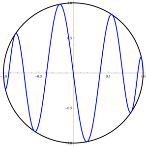
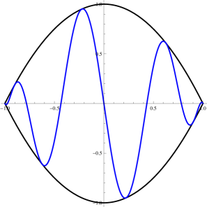
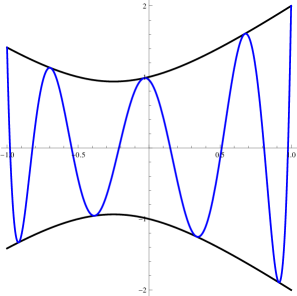
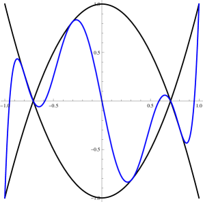
Figure 1: The snake polynomials for various majorants: (a) $\mu(x)=\sqrt{1-x^{2}}\;\;$ (b) $\mu(x)=1-x^{2}\;\;$ (c) $\mu(x)=\sqrt{2x^{2}+x+1}\;\;$ (d) $\mu(x)=|1-2x^{2}|$

Open problem. Find a class of majorants $\mu$ for which the associated snake polynomials $Q_{n}$ have non-negative or sign alternating expansion in the Chebyshev polynomials of the first kind, i.e.

$$Q_{n}=\sum_{i=0}^{n}a_{i}\,T_{i}\ \text{ with all }\ a_{i}\geq 0\ \text{ or with }\ a_{i}\,a_{i+1}<0\ \ \forall\ i.$$

Conjecture (G.N.) If $\mu\geq 0$ is a continuous even convex function in $[-1,1]$, then the associated with $\mu$ snake polynomials have non-negative expansion in the Chebyshev polynomials of the first kind.

The snake polynomials are analogous to the Chebyshev polynomials $T_{n}$ for $\mu\equiv 1$ and are of great interest in relation to the following two problems:

Problem 1: Markov inequality with a majorant Given $n,k\in\mathbb{N}$, $1\leq k\leq n$, and a majorant $\mu\geq 0$, find

$$M_{k,\mu}:=\sup\{\|p^{(k)}\|\,:\,p\in\mathcal{P}_{n},\,|p(x)|\leq\mu(x),\,x\in[-1,1]\}\,.$$

Problem 2: Duffin-Schaeffer inequality with a majorant Given $n,k\in\mathbb{N}$, $1\leq k\leq n$, and a majorant $\mu\geq 0$, find

$$D_{k,\mu}^{*}:=\sup\{\|p^{(k)}\|\,:\,p\in\mathcal{P}_{n},\,|p(x)|\leq\mu(x),\,x\in\delta^{*}\}\,.$$

A conjecture (belonging to mathematical folklore) says that the extremal polynomial to Problem 1 is the snake polynomial $\omega_{\mu}$. So far, no counterexample to this conjecture has been found. On the contrary, $\omega_{\mu}$ is not always the extremal polynomial to Problem 2, the following counterexamples are known:

$$1)\quad\mu(x)=\sqrt{1-x^{2}},\quad k=1;\qquad 2)\quad\mu(x)=1-x^{2},\quad k=1,2\,.$$

In [6, 7] the majorants $\mu$ were studied for which the snake-polynomial $\omega_{\mu}$ is extremal to both Problems 1 and 2, i.e., when equality

$$M_{k,\mu}=D_{k,\mu}^{*}=\|\omega^{(k)}_{\mu}\|\,$$ (3)

holds. It was proved that (3) holds if $\omega_{\mu}$ admits non-negative or sign-alternating expansion in the Chebyshev polynomials, and so the question of our interest is to characterize the corresponding class of measures $\mu$.

Edward Saff

For $-2<s<d$, the Riesz energy of a probability measure $\mu$ on $\mathbb{R}^{d}$ is

$$I_{s}(\mu):=\iint K_{s}(x-y)d\mu(x)d\mu(y),$$

where $K_{s}(x)$ is the Riesz $s$-kernel defined by $K_{s}(x)=\begin{cases}\frac{1}{s|x|^{s}},\;\;\;\;\;\;\;\;\textnormal{if}\;\;s\neq 0,\\ -\log|x|,\;\;\;\textnormal{if}\;\;s=0.\end{cases}$

Riesz original problem. In [2] Riesz showed that the equilibrium measure

$\mu_{*}:=\mathop{\arg\;\;\min_{\mu}}_{\textnormal{supp}(\mu)\subset B_{R}}\;\;I_{s}(\mu)$ on the ball $B_{R}:=\{x\in\mathbb{R}^{d}:|x|\leq R\}$ is given by

$$\mu_{*}=\begin{cases}\sigma_{R},\hskip 108.405pt\>\quad\quad\quad\textnormal{if}-2<s\leq d-2,\\ \frac{\Gamma(1+\frac{s}{2})}{R^{s}\pi^{\frac{d}{2}}\Gamma(1+\frac{s-d}{2})}\frac{\textbf{1}_{B_{R}}}{(R^{2}-|x|^{2})^{\frac{d-s}{2}}}dx,\;\;\;\;\;\quad\textnormal{if}\;\;0\leq d-2<s<d,\\ \end{cases}$$

where $\sigma_{R}$ is the uniform distribution on sphere of radius $R$.

The math arXiv version (arXiv:2108.00534) of [1] contains in its Appendix D.2 a short alternative proof of the Riesz original problem.

Equilibrium open problem for multi-dimensional annulus. Given $d-2<s<d$, find an equilibrium measure on an annulus $B_{r,R}:=\{x\in\mathbb{R}^{d}:r\leq|x|\leq R\}$, i.e. the measure $\mu_{*}$ such that

$$\mu_{*}=\mathop{\arg\;\;\min_{\mu}}_{\textnormal{supp}(\mu)\subset B_{r,R}}\;\;I_{s}(\mu).$$

Boris Shapiro

1. On shadows of polynomials

In [BHS] my coauthors and I studied asymptotic of root distribution for the polynomial sequences $\{Q_{n,\alpha}(x)\}_{n=1}^{\infty}$ where

$$Q_{n,\alpha}(x)=\frac{d^{[\alpha n]}P^{n}(x)}{dx^{[\alpha n]}}.$$

Here $P(x)$ is a fixed univariate polynomial of degree $d\geq 2$, $\alpha\in(0,d)$ and $[\alpha n]$ stands for the integer part of $\alpha n$.

Motivated by the set-up of [BHS] and the famous Gauss-Lucas theorem, let us consider the double-indexed polynomial family

$$Q_{n,m}(x)=\frac{d^{m}P^{n}(x)}{dx^{m}},$$

where $0\leq m\leq nd$. Obviously, for any pair of non-negative integers $(n,m)$, all roots of $Q_{n,m}(x)$ (if any) lie in the convex hull of the roots of $P(x)$. Consider the union of all roots of all $Q_{n,m}(x)$ with $0\leq m\leq nd$ and denote the closure of the latter countable set as $\Upsilon_{P}$ – the shadow of the polynomial $P(z)$. Numerical examples of shadows for polynomials of different degrees are shown in Fig. 2.

Conjecture 1.

For any polynomial $P$ of degree at least $3$ whose roots are in convex position, but do not form a regular polygon,

(i) $\Upsilon_{P}$ is a closed domain in the convex hull of the roots of $P$.

(ii) All critical points of $P$ lie on the boundary of $\Upsilon_{P}$.

(iii) the boundary of $\Upsilon_{P}$ has no inflection points.

(iv) The boundary of $\Upsilon_{P}$ is contained in the union of all critical values (w.r.t. $z$) of the rational function

$$F_{\boldsymbol{\alpha}(z)}=z-\boldsymbol{\alpha}\frac{P(z)}{P^{\prime}(z)}.$$ (4)

where the parameter $\boldsymbol{\alpha}$ runs over the interval $[0,d]$.

Remark 1.

Item (iii) can be reformulates as follows. The boundary of $\Upsilon_{P}$ consists of all $u$ for which the family $\tilde{\Phi}(\boldsymbol{\alpha},z,u)=\boldsymbol{\alpha}P(z)+(u-z)P^{\prime}(z)$ has a multiple root w.r.t. $z$ when $\boldsymbol{\alpha}\in[0,d]$.

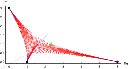
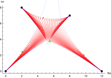
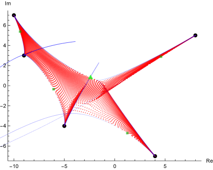
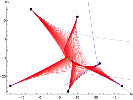
Figure 2: The union of all zeros of $Q_{30,m}(z)$ for $m=0,1,$ $\dotsc,30\deg{P}-1$ shown by small red dots. The large black dots are the zeros of $P$, the green squares are the critical points of $P$, the green triangle is the center of mass of the zero locus of $P$.

It seems that the shadow $\Upsilon_{P}$ is a very natural and interesting domain on whose boundary lie the critical points of $P$. It can also considered as the support of an asymptotic root-counting measure which is worth studying in its own rights.

2. On Maxwell’s problem

In [GNSh] my coauthors and I have been discussing the following ”result” which they found in [Ma].

Conjecture 2 (J. C. Maxwell).

For any configuration of $N$ fixed electric charges in $\mathbb{R}^{3}$ having finitely many points of equilibrium, the number of the latter points is at most $(N-1)^{2}$.

Remark 2.

Observe that almost all configurations of fixed point charges satisfy the assumptions of the above conjecture that their number of points of equilibrium is finite.

The following folklore claim is widely open.

Conjecture 3.

Any configuration of $N$ positive electric charges in $\mathbb{R}^{d}$ has only finitely many points of equilibrium.

In [GNSh] we were only able to prove a very bad upper bound for the number of points of equilibrium however in a more general situation. Since then our upper bound has been improved in a number of very special cases. The best general improvement has been made in a recent preprint [Zo]. However Conjecture 2 is still open even for $n=3$.

References

- [1] C. Tracy, H. Widom, Level-spacing distributions and the Airy kernel, Commun. Math. Phys. 159(1):151-174 (1994).
Dmitrii Karp333E-mail: D. Karp – dimkrp@gmail.com

References

- [1] D.Karp, Positivity of Toeplitz determinants formed by rising factorial series and properties of related polynomials, Journal of Mathematical Sciences, 2013, Volume 193, Issue 1, 106-114. https:dx.doi.org/10.1007/s10958-013-1438-y
- [2] D.B.Karp and E.G.Prilepkina, Alternative approach to Miller-Paris transformations and their extensions, pp.117-140 in Transmutation Operators and Applications (edited by V.V.Kravchenko and S.M.Sitnik), Springer Trends in Mathematics Series, Birkhäuser, 2020. https://doi.org/10.1007/978-3-030-35914-0_6
- [3] A. Martinez-Finkelshtein, R. Morales, D. Perales, Real roots of hypergeometric polynomials via finite free convolution https://arxiv.org/abs/2309.10970
- [4] A. Sokal, When does a hypergeometric function belong to the Laguerre–Pólya class ? J. Math.Anal.Appl.515 (2022) 126432. https://doi.org/10.1016/j.jmaa.2022.126432
Arno Kuijlaars444E-mail: A. Kuijlaars – arno.kuijlaars@kuleuven.be

References

- [1] F. Balogh, M. Bertola, S.Y. Lee, and K.D.T-R McLaughlin, Strong asymptotics of the orthogonal polynomials with respect to a measure supported on the plane, Comm. Pure Appl. Math. 68 (2015), 112–172.
- [2] P. Elbau and G. Felder, Density of eigenvalues of random normal matrices, Comm. Math. Phys. 259 (2005), 433–450.
- [3] E.B. Saff and V. Totik, Logarithmic Potentials with External Fields, Springer Verlag, Berlin, 1997.
Geno Nikolov555E-mail: G. Nikolov – geno@fmi.uni-sofia.bg

References

- [1]
- [2] G. Nikolov, On certain Duffin and Schaeffer type inequalities, J. Approx. Theory 93 (1998), 157–176
- [3] G. Nikolov, Inequalities of Duffin-Schaeffer type, SIAM J. Math. Anal. 33(2001), no. 3, 686–698
- [4] G. Nikolov, Snake polynomials and Markov-type inequalities, in: Approximation Theory: A volume dedicated to Blagovest Sendov (B. Bojanov, ed.), pp. 342–352, DARBA, Sofia, 2002
- [5] G. Nikolov, Inequalities of Duffin-Schaeffer type, II, East J. Approx. 11(2005), no. 2, 147–168
- [6] G. Nikolov, A. Shadrin, On Markov-Duffin-Schaeffer Inequalities with a Majorant, in: Constructive Theory of Functions. Sozopol, June 3–10, 2010. In Memory of Borislav Bojanov, pp. 227–264 http://www.math.bas.bg/mathmod/Proceedings_CTF
- [7] G. Nikolov, A. Shadrin, On Markov-Duffin-Schaeffer Inequalities with a Majorant, II, in: Constructive Theory of Functions. Sozopol, June 9–14, 2013. Dedicated to Blagovest Sendov and to the memory of Vasil Popov, pp. 175–97 http://www.math.bas.bg/mathmod/Proceedings_CTF
Edward Saff666E-mail: E. Saff – edward.b.saff@vanderbilt.edu
Equilibrium measure on an annulus

References

- [1] D. Chafaï, E.B. Saff, R.S. Womersley, On the solution of a Riesz equilibrium problem and integral identities for special functions, J. Math. Anal. and App., Volume 515, Issue 1, 1 November 2022, 126367
- [2] M. Riesz, Intégrales de Riemann–Liouville et potentiels Acta Sci. Math. Szeged 9 (1938): 1–42, 116–118
- [3] E. B. Saff, V. Totik, Logarithmic Potentials with External Fields, Berlin: Springer-Verlag, 1997.
Boris Shapiro777E-mail: B. Shapiro – shapiro@math.su.se

References

- [BHS] R. Bøgvad, Ch. Hägg, B. Shapiro, Rodrigues’ descendants of a polynomial and Boutroux curves, Constructive Approximation, DOI 10.1007/s00365-023-09657-x.
- [GNSh] A. Gabrielov, D. Novikov, and B. Shapiro, Mystery of point charges, Proc. London Math. Soc. (3) vol 95, issue 2 (2007) 443–472.
- [Ma] J. C. Maxwell, A treatise on electricity and magnetism, vol. 1, republication of the 3rd revised edition (Dover, New York, 1954).
- [Zo] Vl. Zolotov, Upper bounds for the number of isolated critical points via Thom-Milnor theorem, arXiv:2307.00312.