A Galactic Eclipse: The Small Magellanic Cloud is Forming Stars in Two, Superimposed Systems

Abstract

The structure and dynamics of the star-forming disk of the Small Magellanic Cloud (SMC) have long confounded us. The SMC is widely used as a prototype for galactic physics at low-metallicity, and yet we fundamentally lack an understanding of the structure of its interstellar medium (ISM). In this work, we present a new model for the SMC by comparing the kinematics of young, massive stars with the structure of the ISM traced by high-resolution observations of neutral atomic hydrogen (Hi) from the Galactic Australian Square Kilometer Array Pathfinder survey (GASKAP-Hi). Specifically, we identify thousands of young, massive stars with precise radial velocity constraints from the Gaia and APOGEE surveys and match these stars to the ISM structures in which they likely formed. By comparing the average dust extinction towards these stars, we find evidence that the SMC is composed of two structures with distinct stellar and gaseous chemical compositions. We construct a simple model that successfully reproduces the observations and shows that the ISM of the SMC is arranged into two, superimposed, star-forming systems with similar gas mass separated by $\sim 5\rm\,kpc$ along the line of sight.

1 Introduction

As one of our nearest neighbors, the Small Magellanic Cloud (SMC) is among the most highly scrutinized galaxies in the Universe. Located at a distance of $\sim 62$ kpc (see compliation of historical estimates in de Grijs & Bono, 2015), the SMC is close enough that individual stars and interstellar medium (ISM) structures can be resolved.

What makes the SMC especially interesting is its markedly different interstellar conditions to the Milky Way. In particular, the SMC has a low metallicity ($\sim 20\%$ Solar; Russell & Dopita, 1992), making it an excellent laboratory for deciphering the physics of the ISM at higher redshift (e.g., cosmic noon), where similar pristine conditions are expected to be prevalent.

However, the line of sight structure of the SMC is not well constrained, due in large part to the fact that different observational tracers paint disparate pictures for its geometry. For example, the oldest stellar populations in the SMC are distributed spherically within a radius of $7-12\rm\,kpc$ (Subramanian & Subramaniam, 2012), and do not show significant signs of rotation (Harris & Zaritsky, 2006; Gaia Collaboration et al., 2018a; Niederhofer et al., 2018; Zivick et al., 2018; Niederhofer et al., 2021), except for in the very central region (within $\pm 1\rm\,kpc$ from the SMC optical center; Zivick et al., 2021). Stars with measurable distances (red clump stars, Cepheid variables, RR Lyrae) are greatly dispersed along the line of sight ($\sim 20-30\rm\,kpc$ depth; Mathewson et al., 1988; Nidever et al., 2013; Scowcroft et al., 2016; Jacyszyn-Dobrzeniecka et al., 2016; Ripepi et al., 2017). In contrast, young main sequence and red giant branch (RGB) stars display a radial velocity gradient indicative of rotation (Evans & Howarth, 2008; Dobbie et al., 2014; El Youssoufi et al., 2023). In addition, the velocity distribution of stars in the central SMC exhibits signs of tidal disruption at the hands of the Large Magellanic Cloud (LMC) (Niederhofer et al., 2018; Zivick et al., 2019; De Leo et al., 2020; Zivick et al., 2021; Niederhofer et al., 2021). There is mounting evidence for the presence of distinct substructures along the line of sight (e.g., Hatzidimitriou & Hawkins, 1989; Martínez-Delgado et al., 2019; Cullinane et al., 2023). In addition, there is a well-known “bimodality” in distance observed in red clump stars on the Eastern side of the system (e.g., Nidever et al., 2013) and recently traced throughout the SMC (Subramanian et al., 2017; Tatton et al., 2021; Omkumar et al., 2021; Almeida et al., 2023). Furthermore, recent chemical analysis of RGB stars in the SMC exhibit complex distributions in both radial velocity and metallicity ([Fe/H]), suggesting that chemical enrichment in the system “has not been uniform”, pointing to either strong influence of star formation (SF) bursts (Hasselquist et al., 2021; Massana et al., 2022) or chemically distinct substructures (Mucciarelli et al., 2023).

Figure 1: Top: Intensity-weighted mean velocity map of the SMC from Pingel et al. (2022). The single contour indicates an Hi column density of $15\times 10^{20}\rm\,cm^{-2}$. The center of the SMC used in this work (defined based on the stellar populations observed by Gaia Zivick et al., 2021) is marked with a magenta cross. Spatial bins are overlaid and identified with numbers. Bottom: The average Hi brightness temperature spectra ($T_{b}(v_{r})$) profiles from spatial bins marked at left (black). Each panel includes shaded grey envelopes denoting the $16^{\rm th}$ through $84^{\rm th}$ percentile of the $T_{b}(v_{r})$ within each spatial bin. We observe that the radial velocity structure of Hi emission features multiple, distinct velocity peaks (and typically two, dominant components).

In addition to its diversely structured stellar populations, the ISM of the SMC is highly disturbed (Stanimirović et al., 1999). Neutral hydrogen (Hi) emission in the SMC is organized into multiple, distinct peaks in radial velocity. This structure was originally interpreted as the presence of two, distinct sub-systems separated in space (Kerr et al., 1954; Johnson, 1961; Hindman, 1964). Mathewson & Ford (1984) further showed that the velocities of stars, HII regions and planetary nebulae matched that of the Hi, and concluded that the SMC has been “badly torn” by its interactions with the LMC, in agreement with the leading theoretical models at that time (Murai & Fujimoto, 1980). The widely held interpretation is that the low velocity gas must be in front (Hindman, 1964; Mathewson & Ford, 1984), given that optical absorption is typically associated with the low-velocity Hi peak (e.g., Danforth et al., 2002; Welty et al., 2012). But the interpretation of these results has not always necessitated the presence of two distinct components. For example, a recent study of gaseous filaments in the SMC establishes that the filaments in the low and high velocity components show a preference for being aligned with each other, which suggests that they must somehow be physically related (Ma et al., 2023). Another alternative interpretation is that the system is a series of overlapping supershells (Hindman, 1967; Staveley-Smith et al., 1997).

Despite this complexity, the line-of-sight integrated Hi velocity field of the SMC is broadly consistent with a rotating disk (Stanimirović et al., 2004; Di Teodoro et al., 2019). This disk model has underpinned our concept of the SMC system and has long-defined its total dynamical mass – a key ingredient to numerical simulations. However, the velocity gradient observed in Hi emission is perpendicular to that observed in the radial velocities of young stars (Evans & Howarth, 2008; Dobbie et al., 2014). In addition, the distance gradient observed in Cepheids from the North East to South West is oriented $\sim 90$ degrees away from the minor axis of the gas disk (Scowcroft et al., 2016). Finally, the 3D kinematics of young, massive stars throughout the SMC, which are young enough to trace the kinematics of their birth clouds in the ISM, are inconsistent with the disk rotation model (Murray et al., 2019).

These observational inconsistencies have traditionally been explained away by the fact that the SMC has been severely disrupted by its recent interactions with the nearby LMC. Although precise observations of stellar proper motions in the LMC and SMC (Kallivayalil et al., 2006b, a; Besla et al., 2007; Piatek et al., 2008; Zivick et al., 2018) indicate that the LMC and SMC are likely on their first infall into the Milky Way (MW) halo (although a second infall scenario is also possible; Vasiliev, 2024), spatially-resolved star formation histories show that the two galaxies have been interacting with each other repeatedly for the past several Gyr (e.g., Massana et al., 2022). These interactions have produced a wealth of debris in the outskirts of both Clouds (Besla et al., 2016; Mackey et al., 2016; Belokurov et al., 2016; Carrera et al., 2017; Pieres et al., 2017; Choi et al., 2018; Martínez-Delgado et al., 2019). In particular, the Clouds likely made a direct collision $\sim 150$ Myr ago (Zivick et al., 2021; Choi et al., 2022). These interactions have produced the massive, gaseous debris fields known as the Leading Arm, Bridge and Stream (Wannier et al., 1972; Mathewson et al., 1974; Putman et al., 1998; Nidever et al., 2010; For et al., 2014, 2016).

As the more massive of the two galaxies by a factor of $\sim 10$ (Peñarrubia et al., 2016; Erkal et al., 2019), the LMC has survived this eventful interaction history as a nearly face-on rotating disk (van der Marel & Kallivayalil, 2014; Gaia Collaboration et al., 2021). As a result, theoretical efforts to reconstruct the formation history of the broader Magellanic System (MS) largely focus on the interaction between the LMC and MW (e.g., Besla et al., 2012; Pardy et al., 2018; Lucchini et al., 2021). However, constraining the precise orbital histories (and futures) of the MCs and their satellites relies on the influence of the SMC (Patel et al., 2020). It is thus critical to develop a model that reconciles these diverse observational constraints.

In this work, we present a new model for gas in the SMC, and show that it is composed of not one, but two structures located at distinct distances along the line of sight, distributed across the inner $\pm 4^{\circ}$ of the SMC. In Section 2, we discuss the data products used in our analysis. In Section 3, we present our analysis procedure, in which we determine the order of ISM components along the line of sight. In Section 4, we present a toy model to describe our observational results. In Section 5, we discuss this new model in the context of the literature and the history of the MS. Finally, we conclude in Section 6.

2 Data

In this section, we describe the data products used in our analysis. Specifically, we will combine information from the following sources:

• High-resolution observations of the SMC’s neutral gas emission at $21\rm\,cm$ from the GASKAP-Hi survey (Pingel et al., 2022), which trace the radial velocity of the bulk gas population in the system.

• Line of sight extinction and radial velocity measurements of bright, young ($10-100$ Myr) stars in the SMC from the Gaia mission DR3 (Gaia Collaboration et al., 2016, 2023; Babusiaux et al., 2023) and APOGEE DR17 (Majewski et al., 2017; Zasowski et al., 2017; Abdurro’uf et al., 2022).

We also use supplementary information from the APOGEE spectral fits, as well as large-area molecular gas observations of the system to assess its chemical state.

2.1 Neutral gas radial velocities

The ISM of the SMC is heavily dominated by atomic gas (Leroy et al., 2007; Jameson et al., 2016), and therefore to trace the bulk distribution of gas, we use the recent survey of 21 cm emission in the SMC from the Galactic Australian Square Kilometer Array Pathfinder (GASKAP-Hi) collaboration (Pingel et al., 2022). This dataset was constructed from 20.9 hours of integration time by ASKAP (Hotan et al., 2021) on the SMC ($\rm RA=00h58m43.280s,Dec=-72d31m49.03s$) in December 2019. ASKAP is composed of 36 antennas, each equipped with a phased array feed receiver which combine to give the telescope an instantaneous field of view of $\sim 25$ square degrees (Hotan et al., 2021). The resulting data products were combined with single-dish observations from the GASS survey (McClure-Griffiths et al., 2009; Kalberla et al., 2010; Kalberla & Haud, 2015) to produce an Hi emission data cube with an angular resolution of $30^{\prime\prime}$ ($\sim 10$ pc at a distance of $62\rm\,kpc$), sensitivity to Hi brightness temperature of $1.1\rm\,K$ and a per-channel velocity resolution of $0.98\rm\,km\,s^{-1}$ – by far the highest-resolution, fully-resolved Hi survey of the SMC to date (Pingel et al., 2022).

Figure 2: CMDs of the Gaia (a) and APOGEE (b) samples (before RSG selection). Black contours in each panel denote the $1$, $2$ and $3\sigma$ limits of the total Gaia SMC sample. Red supergiants (RSGs) are indicated by the blue highlighted region in each panel. (c) Spatial distribution of selected RSG stars for the Gaia and APOGEE samples. The Hi distribution is highlighted by a single gray contour at $15\times 10^{20}\rm\,cm^{-2}$ (see Figure 1).

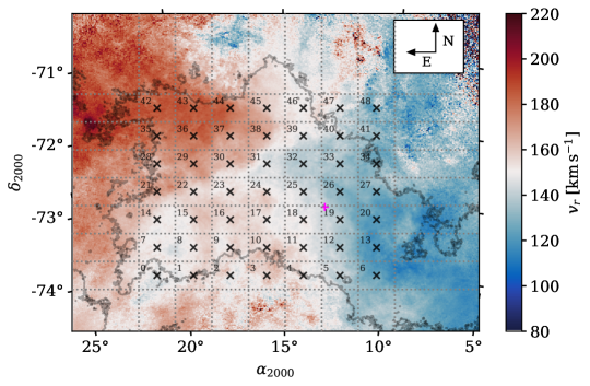
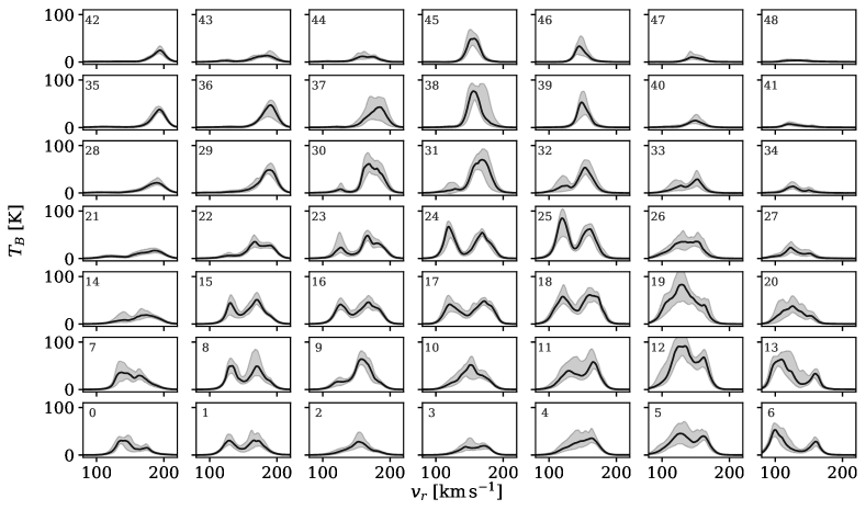
In Figure 1, we display the intensity-weighted mean radial velocity of the GASKAP-Hi cube (a.k.a., the first moment) for visualization of the velocity structure of gas in the SMC. There is a clear gradient in radial velocity across the main body of the SMC, which seems to resemble the signature of a rotating disk (e.g., Di Teodoro et al., 2019; Gerrard et al., 2023). In the right-hand panel of Figure 1, we display example brightness temperature spectra ($T_{B}(v)$) drawn from a regular grid of positions overlaid on the first moment map. We observe that these example spectra display complex, multi-peaked structure. In particular, across the main body of the SMC, where we see strong emission, there are often two distinct spectral components, one at high velocity ($\sim 170\rm\,km\,s^{-1}$) and one at low velocity ($\sim 130\rm\,km\,s^{-1}$).

2.2 Line-of-sight extinction and radial velocity of embedded stars

Although 21 cm emission provides a high-resolution probe of the position-position-velocity structure of the gas, it does not directly probe the line of sight distance axis. To sample this third spatial dimension, we use measurements of extinction by dust toward individual stars. As extinction provides a cumulative measurement of the effect of dust along the line of sight, we can compare extinction values towards stars at different radial velocities in order to determine the relative spatial order of these stars along the line of sight (i.e., “front” and “behind”).

As our primary goal is to connect the line of sight structure of the stars with the radial velocity structure of the gas, we make the assumption that the gas, the dust, and the young stars coexist spatially and share bulk kinematics on the same spatial scales probed by each tracer. With these assumptions, we can compare total extinction measured to samples of stars with different radial velocities in order to determine the relative order along the line of sight. Although the assumption that dust and gas are well-mixed is widely accepted, the assumption that the stars trace the same 3D motions as the gas relies on targeting only the youngest stellar populations, whose lives are short enough that their motions are coupled to the motions of their parent gas clouds (e.g., Großschedl et al., 2021). The precise definition of “young” to satisfy this requirement is not well-defined, especially in the low-metallicity, dynamically complex environment of the SMC. In general, stellar populations will lose memory of their birthplaces on a dynamical timescale (i.e., a crossing timescale of about $100\rm\,Myr$ for the SMC). As we will describe below, we endeavor to select stars young enough (ages $\sim 10$s of Myr) such that our assumption is valid when averaged across large spatial areas, rather than in individual cases.

For this study, we assemble SMC stars observed by the APOGEE survey and the Gaia mission. Both products include precise radial velocity measurements for thousands of stars, and their selection is described below.

2.2.1 Gaia

To construct an initial sample of SMC stars from Gaia DR3 (Gaia Collaboration et al., 2016, 2023; Babusiaux et al., 2023), we follow the strategy described by Gaia Collaboration et al. (2018b). First, to construct a proper motion filter for SMC stars, we select all stars from DR3 within $3^{\circ}$ of $(\alpha_{2000},\delta_{2000})=(13.15833^{\circ},-72.8002^{\circ})$ with low parallax over error ($\varpi/\sigma_{\varpi}<10$) to minimize foreground contamination. Following Equation 2 of Gaia Collaboration et al. (2018b), we compute the orthographic projections of the source coordinates, and further select all stars with mean G-band magnitude $G<19\rm\,mag$. Next, we compute the median proper motions of these stars in $x$ and $y$ ($\mu_{x}$ and $\mu_{y}$), and exclude all stars with values beyond $4\times$ the robust scatter estimate (Gaia Collaboration et al., 2018b) from the median in both axes. Then, we compute the covariance matrix of $\mu_{x},\,\mu_{y}$ ($\sigma$) and ultimately define a filter on proper motions defined as $\mu^{T}\sigma^{-1}\mu<9.21$. We acknowledge that genuine SMC stars may be excluded by this cut, as stars outside the inner $3^{\circ}$ may have significantly different proper motions. However, we estimate this to be a small effect on our analysis as our focus is on young stars with kinematics consistent with the bulk SMC population.

To select a complete sample of SMC stars, we select all stars within $8^{\circ}$ of the SMC center (although this is larger than the GASKAP-Hi footprint, here we simply follow the previous analysis of Gaia Collaboration et al. (2018b)) with $\varpi/\sigma_{\varpi}<10$ and $G<20$, and apply the proper motion filter defined on the central regions of the SMC above to produce a catalog of 2,006,326 SMC stars. As a last step, we restrict this catalog to the footprint of the GASKAP-Hi SMC cube, yielding 1,687,195 stars.

Since our primary interest is to use stars to probe the velocity structure of gas in the system, we further select only stars with radial velocity measurements from Gaia. This removes the majority of stars in our initial SMC/GASKAP-Hi sample, as radial velocities are only measurable at the SMC distance for the brightest stars. In total, we have 3,783 stars with radial velocities. From these, we select only those within the SMC velocity range ($80<v_{r}<250\rm\,km\,s^{-1}$; 3,707 stars). Finally, we convert the Gaia radial velocities from their native barycentric reference frame to the Local Standard of Rest frame to be consistent with the Hi.

Figure 3: Ages of synthetic stellar populations with a range of SMC-like metallicities. We compare synthetic stars passing our RSG selection criteria (Figure 2) with synthetic stars in the RGB, AGB and “blue loop” (BL) (the selection of these populations in color-magnitude space is defined in Section 2.3.2 of Gaia Collaboration et al., 2021). We note that the blue loop sample (BL) overlaps with the RSG selection in Figure 1.

2.2.2 APOGEE

In addition to the Gaia stars, we select stars from the second iteration of the Apache Point Observatory Galactic Evolution Experiment (APOGEE-2, Majewski et al. 2017), which was a part of the fourth iteration of the Sloan Digital Sky Survey (SDSS-IV, Blanton et al. 2017). APOGEE-2 consisted of two $H$-band spectrographs (Wilson et al., 2019), one on the SDSS 2.5m telescope at Apache Point Observatory (Gunn et al., 2006) and one on the 2.5m du Pont Telescope at Las Campanas Observatory (Bowen & Vaughan, 1973), the latter of which allows for observations of the SMC due to its position in the Southern hemisphere. SMC stars were targeted through a combination of main survey fields and special fields from “Contributed Programs”, as described and detailed in Zasowski et al. (2017); Nidever et al. (2020); Santana et al. (2021).

In this work, we make use of APOGEE radial velocities and metallicities from the 17th Data Release (DR17) of SDSS-IV (Abdurro’uf et al., 2022). APOGEE measures radial velocities by cross-correlating the observed spectra with synthetic spectra, using methodology described in detail in Nidever et al. (2015) and updates described in Abdurro’uf et al. (2022). Jönsson et al. (2020) found that the APOGEE DR16 radial velocities agreed with Gaia DR2 to within $1-2\rm\,km\,s^{-1}$ depending on the apparent magnitude of the star. We find similar agreement. For the 548 stars in common between APOGEE and Gaia, the RVs agree to within $0.03^{+2.2}_{-1.6}\rm\,km\,s^{-1}$ (mean and $\pm 1\sigma$ errors), which is comparable to the average uncertainty in radial velocity in the Gaia sample of $1.5\rm\,km\,s^{-1}$. APOGEE metallicities are measured using the APOGEE Stellar Parameters and Chemical Abundance Pipeline (ASPCAP, García Pérez et al. 2016), which uses the FERRE code (Allende Prieto et al. 2006) to match the normalized, RV-corrected, and sky-subtracted spectra to a library of synthetic stellar spectra, the generation of which is described in Zamora et al. (2015). Updates to this spectral grid are described in Abdurro’uf et al. (2022), which include spectral grids generated using the SYNSPEC code (Hubeny et al., 2021) with non-local thermodynamic equilibrium corrections from Osorio et al. (2020).

Figure 4: Synthetic IR color histograms for three subsets of the simulated stellar population: all (black), those passing our Gaia color selection for RSGs (blue), and those passing the Gaia color selection for RGBs defined in (Gaia Collaboration et al., 2021) (red). We observe that the simulated RSGs span an even narrower $H-4.5\mu$m distribution than the RGBs.

Figure 5: Average radial velocity of the selected stellar catalog from Gaia and APOGEE ($v_{r}$, LSR) (binned spatially according to the pixel sizes shown). The stars display a radial velocity gradient across the main body of the SMC with similar magnitude as the gas (Figure 1).

We select all APOGEE stars within a radius of $9^{\circ}$ from the SMC center (5,938 stars). This search radius is significantly larger than the GASAKP-Hi footprint, and therefore is aribitrarily selected. We then compute the proper motions in $x$ and $y$ in the same way as for the Gaia sample and exclude all stars with values beyond $4\times$ the robust scatter estimate (Gaia Collaboration et al., 2018b) from the median of the Gaia sample in both axes. We then convert the Heliocentric velocities from APOGEE to the LSR frame and select stars with SMC velocities ($80<v_{r}<250\rm\,km\,s^{-1}$) residing within the GASKAP-Hi footprint (2,407 stars).

Figure 6: $A_{K}$ versus velocity for stars within the same regularly-spaced spatial bins as in Figure 1. The stars are colored by the radial velocity according to the same colorbar as in Figure 1. The average Hi $T_{b}(v_{r})$ profiles are overlaid in black, and include shaded grey envelopes denoting the $16^{\rm th}$ through $84^{\rm th}$ percentiles of the $T_{b}(v_{r})$ within each spatial bin. In general, the stellar radial velocities span the same range as the Hi velocities across the SMC.

2.2.3 Young star selection

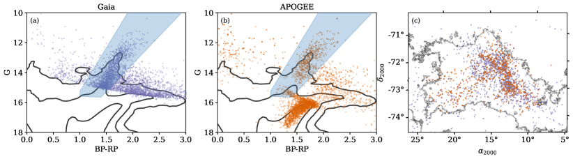
In Figure 2, we display color-magnitude diagrams (CMDs) for the two samples. We use the Gaia observed magnitudes, $BP$-$RP$ (a blue-red color index) and $G$.

In the case of the Gaia sample, the stars with measured radial velocities are all bright ($G\lesssim 16$). In both samples, the stars span a wide range of stellar types, including pulsating variables, red supergiants, and asymptotic giant branch stars (Gaia Collaboration et al., 2021).

The APOGEE stars span a wider range in magnitude, as this survey included both shallow and deep observations. As a result there is a gap between the faintest and brightest RSGs around $G\sim 15$. We will discuss the effect of the magnitude distribution of this sample on our results in Section 3.

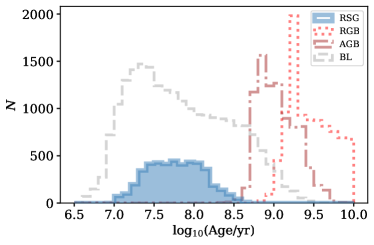
From these stars, we need to sub-select according to two conditions: (1) stars that are young enough to support our assumption that their motions trace the bulk motions of their parent gas clouds; (2) stars of a spectral type that is well-understood enough for the line of sight extinction towards them to be accurately inferred with available data. To satisfy these criteria, we select all stars within the region highlighted in Figure 2, as this region of the CMD is dominated by RSGs. As a test of our assumption, we generate a set of synthetic stellar isochrone tables for a range of SMC metallicities ([M/H] = $-1.0$ to $-0.65$) from PARSEC (Bressan et al., 2012; Tang et al., 2014; Chen et al., 2014, 2015; Marigo et al., 2017; Pastorelli et al., 2019, 2020). In Figure 3, we plot histograms of the ages of stars in our RSG selection (blue), as well as the ages of a range of stellar populations identified in the SMC by Gaia Collaboration et al. (2021), including red giant branch stars (RGB), asymptotic giant branch stars (AGB), and blue loop stars (BL). The RSG are of intermediate age ($\sim 10-100$ Myr), but are among the youngest stars available in the two surveys. In addition, RSGs in the LMC have been shown to closely mimic the kinematics of the Hi (Olsen et al., 2015).

Following the RSG selection, we combine the Gaia and APOGEE samples by cross-matching the catalogs and removing overlapping stars from the Gaia catalog, yielding a total of 1,947 stars (782 APOGEE, 1,165 Gaia). In Figure 2c, we plot the spatial distribution of these samples. Because the APOGEE survey of the SMC was limited to individual pointings, these stars are not uniformly spread across the galaxy as the Gaia stars. We will discuss the effect of the difference in spatial sampling in Section 3.

2.2.4 Estimating Extinction

To estimate the extinction towards each source in the sample in the same manner, we use the “Rayleigh Jeans Color Excess” (RJCE) method (Majewski et al., 2011). RJCE was developed to quantify the amount of reddening towards individual stars based on a single observed color, $H-4.5\rm\,\mu m$. These wavelengths sample the Rayleigh-Jeans tail of the stellar SED where red clump and red giant stars have the same intrinsic color. As a result, variations in their observed colors can be attributed to the effect of dust extinction (Majewski et al., 2011).

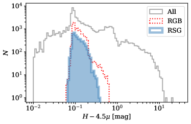
We note that the RJCE method has not been explicitly validated on the stellar types selected here (RSG). To test the validity of the method, we use the same set of synthetic isochrones from Figure 3 and plot histograms of the $H-4.5\mu$m colors for the RSG sample, compared with the RGB sample (where the color-magnitude selection for SMC RGB is defined in Gaia Collaboration et al., 2021) in Figure 4. We observe here that our RSG selected stars span an even narrower $H-4.5\mu$m color range than the RGB stars, granting us confidence that these stars are likely good candidates for the RJCE method.

To compute extinction in $K_{s}$ band, $A_{K}$, we cross-match our sample with the catalog of stars from the Spitzer SAGE-SMC survey (Gordon et al., 2011), specifically the “more reliable” catalog of IRAC Epoch 0, 1, and 2 catalog. This catalog includes IRAC $4.5\mu\rm m$ photometry, as well as $H$-band photometry from 2MASS (Skrutskie et al., 2006). We find a match within a search radius of $3^{\prime\prime}$ for 1,934 of our stars. We then compute the extinction in the $K_{s}$ band, $A_{K}$, using RJCE via Majewski et al. (2011) Equation 1, reproduced here,

$$A_{K}=0.918\,(H-[4.5\mu]-0.08).$$ (1)

We remove stars with NaN-values (117 stars) or extraneously red $3.6-4.5\mu\rm m$ colors (defined as $[3.6-4.5]>0.15$; 10 stars). Our final catalog has 1,801 stars.

Figure 7: Cartoon schematic of the differential extinction estimation process. Top: The average extinction towards stars with “low velocity” ($v_{r}<M_{1}$) is less than the average extinction towards stars with “high velocity” ($v_{r}>M_{1}$) – therefore, $\Delta A_{K}<0$ and the “low velocity” gas component is in front of the high velocity component in this direction. Bottom: The average extinction towards stars with “low velocity” ($v_{r}<M_{1}$) is greater than the average extinction towards stars with “high velocity” ($v_{r}>M_{1}$)– therefore, $\Delta A_{K}>0$ and the “low velocity” gas component is behind the high velocity component in this direction.

Figure 8: The difference in extinction towards low velocity gas and high velocity gas ($\langle\Delta A_{K}\rangle$), averaged across binning parameters at the location of each source. The symbol sizes are scaled by the signal to noise in $\langle\Delta A_{K}\rangle$ (larger symbols = more confidence). The assumed center of the SMC is marked with an “x” ($\alpha_{0},\delta_{0}=13.15833,\,-72.80028$ Zivick et al., 2021) and the direction towards the LMC is indicated with an arrow.

To further validate our measurements, we compare $A_{K}$ with the results of Zhang et al. (2023), who estimated stellar parameters and extinction towards the $220$ million stars with XP spectra from Gaia DR3 using a forward-modeling approach trained on the LAMOST spectral library. We find that the values of $A_{K}$ are positively correlated with the extinction parameter, $E$ (i.e., a scalar proportional to total extinction), from Zhang et al. (2023) with high significance (Pearson $R=0.52$) and the null hypothesis that the two samples are uncorrelated can be rejected with $p\ll 0.001$.

Figure 9: Spatial distribution of stars in the “front” structure ($\langle\Delta A_{K}\rangle<0$ at low velocity and $\langle\Delta A_{K}\rangle>0$ at high velocity) and the “behind” structure ($\langle\Delta A_{K}\rangle>0$ at low velocity and $\langle\Delta A_{K}\rangle<0$ at high velocity). As in Figure 8, the points are scaled by the significance in the $\langle\Delta A_{K}\rangle$ measurement.

We emphasize that, as will be elaborated on in the ensuing analysis, our key metric for this work is a differential measurement in extinction, and therefore the precise zeropoint calibration to the RJCE method are not needed for our analysis. In addition, the correction for Milky Way foreground extinction is not needed, as we assume that the foreground extinction does not vary significantly between spatial bins considered here (see Section 3).

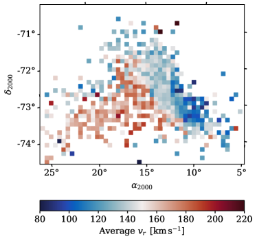
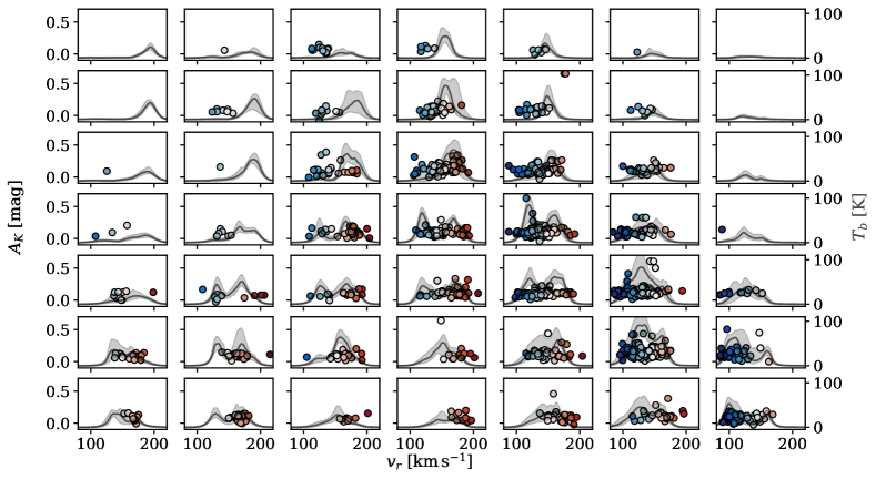
In Figure 5, we plot the spatially-binned average radial velocities of the stars in our sample. The stars are distributed according to the regions of highest Hi column density, and display an East-West gradient in $v_{r}$ with the same magnitude as seen in $T_{b}(v_{r})$ shown in Figure 1. In Figure 6, we plot $A_{K}$ vs. $v_{r}$ for stars in the same example bins shown, and observe that the stars follow the same radial velocity range of the Hi profiles. Of the 1,801 total stars in the sample, 995 ($55\%$) are at low velocity (i.e., $v_{r}<M_{1}$) and 806 are at high velocity.

3 Analysis

The GASKAP-Hi data cube and our selected sample of stars provide two high-resolution probes of the 3D structure of the SMC system. In the following analysis, we match the stars with peaks in $T_{b}(v_{r})$ based on their $v_{r}$ (Figure 1) and compare the average extinction towards the Hi velocity structures observed across the SMC. This differential measurement – the average difference in extinction towards the “low” and “high” velocity peaks observed in Figures 1 – determines the order of these components along the line of sight.

3.1 Matching Stars with Gas

The process of matching the stars with Hi peaks requires a series of selection parameters, which we describe below.

3.1.1 Number of Hi components

To identify the number of Hi components and their properties, we follow Murray et al. (2019), who used the first numerical derivative of the brightness temperature spectrum in each pixel of the Hi data cube from McClure-Griffiths et al. (2018) to identify peaks in radial velocity. In Figure 2 from Murray et al. (2019), they conclude that most of the SMC main body features at least two components. However, in detail, this process requires choosing two free parameters: the minimum $T_{B}$ threshold for a component to be considered “significant” ($T_{B,\rm min}$), and a Gaussian smoothing kernel width ($\sigma_{G}$) for suppressing the effect of spectral noise on the numerical derivative, which is necessary to determine the number of components along the line of sight. We find that varying these selections ($1<T_{b,\rm\,min}<10\rm\,K$, $2<\sigma_{G}<10$) does not have a significant effect on our results, as the majority of the stars are located along high-$T_{b}$, complex LOS. For the ensuing analysis, we select $T_{b,\rm\,min}=5\rm\,K$ and $\sigma_{G}=4$ channels.

Figure 10: Comparing the 3D kinematics ($v_{r}$, $\mu_{W}$ and $\mu_{N}$; left, middle and right, respectively) as a function of Cartesian East-West ($X$) position for stars in the front and behind structures, after subtracting the systemic motions of the SMC. The bottom row of panels compares the binned average values for each velocity component in 10 bins of equal size for the front and behind structures, highlighting in particular the difference in $v_{r}$ as a function of $X$.

3.1.2 Spatial binning of stars

Given that the stellar sample is unevenly distributed across the SMC, with most stars lying in the central regions and far fewer in the outskirts (Figure 2c), we use Voronoi binning (Cappellari & Copin, 2003), an adaptive binning scheme that allows us to ensure consistent source counts across spatial bins. This process also requires several binning parameters. First is the degree of regular-spaced spatial binning before applying the Voronoi binning algorithm (as in practice, using all $\sim 4$ million individual Hi spaxels is prohibitively slow), parameterized by the number of pixels per side per bin ($N_{{\rm pix},V}$). The second free parameter is the signal-to-noise ratio per bin ($\rm(SNR)_{V}$). We select $N_{{\rm pix},V}=30,\,40,\,50,\,60$ and $\rm(SNR)_{V}=3,\,4,\,5,\,6$ and repeat our analysis (below) for each unique combination of these parameters. This allows us to account for the effect of binning choice, while ensuring that there are a uniform number of stars per spatial bin.

3.2 Identifying structures via differential extinction

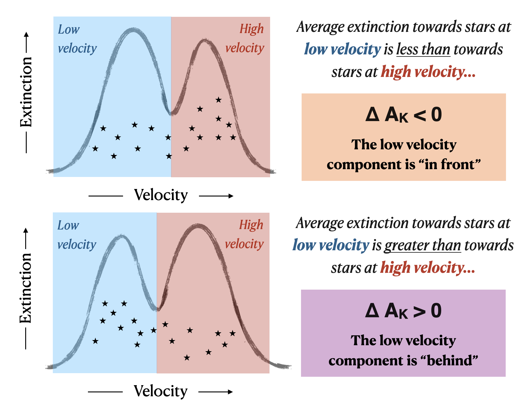
For each combination of selection parameters, in each bin we identify stars at “low” velocity ($v_{r}<M_{1}$) and at “high” velocity ($v_{r}>M_{1}$) where $M_{1}$ is the intensity-weighted average radial velocity of the gas along the line of sight. If there is at least one source in the “low” and “high” velocity samples, we compute the average extinction towards the “low” and “high” samples ($\langle A_{K}\rangle_{\rm low}$, $\langle A_{K}\rangle_{\rm high}$). Finally, we compute the difference between these values, defined as “low” minus “high”:

$$\Delta A_{K}=\langle A_{K}\rangle_{\rm low}-\langle A_{K}\rangle_{\rm high},$$ (2)

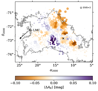
and assign this value of $\Delta A_{K}$ to all stars within the bin. In Figure 7, we illustrate how this process works with simple cartoons for two cases. When $\Delta A_{K}<0$, there is less extinction towards the “low” velocity component than the “high” velocity component, which implies that the low velocity component is in front of the high velocity component. Conversely, when $\Delta A_{K}>0$, there is more extinction towards the low velocity component, which implies that it is behind the high velocity component.

In Figure 8, we plot the average of $\Delta A_{K}$ over all 16 unique combinations of binning parameters for each star ($\langle\Delta A_{K}\rangle$). In each trial, we find that there is a roughly equal number of stars at low and high velocity within each spatial bin, with a total number per bin that ranges between $\sim 6$ and $\sim 40$ stars. In addition, the value of $\langle\Delta A_{K}\rangle$ for each star is derived from a non-uniform (Voronoi) binning scheme which ensures that a different set of stars is selected in each trial. This choice allows us to minimize the impact of single outliers on the results.

We observe clear trends in $\langle\Delta A_{K}\rangle$ across the face of the SMC. The points in Figure 8 have sizes that are scaled by the signal to noise in the measurement of $\langle\Delta A_{K}\rangle$. Given the fact that the dust content of the SMC is diffuse (outside of the major star-forming regions), the magnitude of the extinction difference is small ($\lesssim 0.1\rm\,mag$). However, the fact that the sign of $\langle\Delta A_{K}\rangle$ is constant across large areas ($100\rm s$ of pc, much larger than the spatial bin sizes) indicates that the signal detected at each location is significant.

3.3 Selecting “front” and “behind” samples

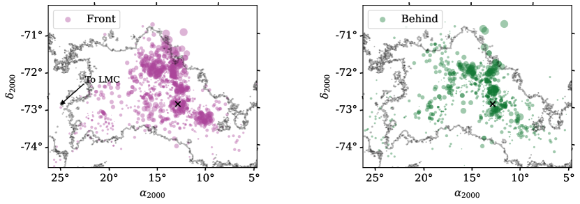
Building from the spatial trends observed in Figure 8, we select all stars in “front” (i.e., negative $\langle\Delta A_{K}\rangle$ at low velocity and positive $\langle\Delta A_{K}\rangle$ at high velocity) and “behind (positive $\langle\Delta A_{K}\rangle$ at low velocity and negative $\langle\Delta A_{K}\rangle$ at high velocity).

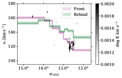
In Figure 9, we plot the spatial distributions of the “front” and “behind” samples. We find 1,014 stars in the front sample and 787 in the behind sample. Of these, $35\%$ and $42\%$ are from APOGEE in the front and behind samples respectively, highlighting the fact that both samples have similar representation from the Gaia-only and APOGEE coverage.

3.4 Kinematics

To analyze the kinematics of the front and behind Hi samples, we first correct for the systemic motion of the SMC. We estimate the mean proper motion of the both the front and behind samples to be $(\mu_{\alpha,\rm sys},\,\mu_{\delta,\rm sys})=(0.77,\,-1.25)\,\rm mas\,yr^{-1}$, which is in good agreement with previous estimates of the proper motion of the SMC (e.g., Jacyszyn-Dobrzeniecka et al., 2017; Zivick et al., 2018). We estimate the systemic radial velocity to be the median of the GASKAP-Hi first moment map, equal to $v_{r,\rm sys}=151\rm\,km\,s^{-1}$. We subtract $v_{r,\rm sys}$, $\mu_{\alpha,\rm sys}$, $\mu_{\delta,\rm sys}$ from $v_{r}$, $\mu_{\alpha}$ and $\mu_{\delta}$ in the sample.

For convenience, we next convert the observed coordinates ($\alpha$, $\delta$) coordinates to a Cartesian frame in the plane of the sky ($X$, $Y$) following van de Ven et al. (2006) Equation 1, reproduced here,

$$X =-r_{0}\,\cos{\delta}\,\sin{\Delta\alpha},$$ (3)

$$Y =r_{0}\,(\sin{\delta}\cos{\delta_{0}}-\cos{\delta}\sin{\delta_{0}}\cos{\Delta\alpha}),$$

where $\Delta\alpha=\alpha-\alpha_{0}$, $\Delta\delta=\delta-\delta_{0}$ and ($\alpha_{0}$, $\delta_{0}$) is the assumed center of the SMC (here, from Zivick et al., 2021). In this frame, positive “$X$” pointing West and positive “$Y$” pointing North. We convert $\mu_{\alpha}$ and $\mu_{\delta}$ to the Cartesian frame ($\mu_{W}$ and $\mu_{N}$) using the orthographic projection from Equation 2 of Gaia Collaboration et al. (2018b), with positive $\mu_{W}$ pointing West and positive $\mu_{N}$ pointing North.

Another important observational effect is “perspective rotation”, or the apparent kinematic signature imposed by the systemic motion of the objects with large angular extent van de Ven et al. (e.g., 2006). Correcting for this effect requires an assumed distance to the star along the line of sight, which in this case is not known. Therefore, we incorporate this correction in when we model our results in Section 4.

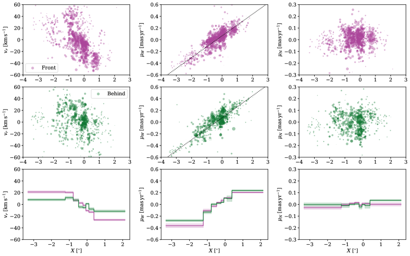
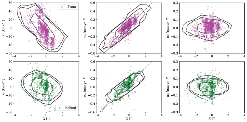
In Figure 10, we plot the three residual (i.e., systemic-corrected) velocities ($v_{r}$, $\mu_{W}$ and $\mu_{N}$) for the stars in each component. In the bottom row, we compare the average values as a function of East-West coordinate ($X$), binned so that there is an equal number of stars per bin.

To compare the velocities between the front and behind samples, we conducted an Anderson-Darling test to compare the distributions of $v_{r}$, $\mu_{W}$ and $\mu_{N}$. The null hypothesis that the two samples are drawn from the same parent population can be rejected with a p-value of $<0.001$ for $v_{r}$, and $0.02$ for $\mu_{W}$ and $\mu_{N}$. This is confirmed visually in Figure 10, it is clear that the slope of the two distributions of $v_{r}$ are significantly different.

In addition, both front and behind display a strong gradient in $\mu_{W}$. We fit a line to this gradient (Figure 10) and find the slope to be $0.185$ ($0.187$) $\rm mas/(yr\,deg)$, with an intercept of $0.068$ ($0.075$) $\rm km\,s^{-1}$, in the front and behind components respectively. This gradient is consistent with being caused by the tidal influence of the LMC on the SMC, which we will discuss further in Section 4.

Figure 11: The residual tangential proper motion ($\mu_{\theta,\rm resid}$) as a function of radius in the front and behind components, after subtracting the gradient in $\mu_{w}$ (Figure 10). Here we plot the average (line) and standard error (shading) in bins of equal numbers of stars (6 bins per sample).

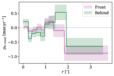
To further explore the residual proper motions in the system, we subtract the gradient in $\mu_{W}$ and look for signatures of rotation in the residuals. To quantify this, we convert $\mu_{W,\rm resid}$ and $\mu_{N}$ to radial and tangential proper motions ($\mu_{r,\rm resid}$ and $\mu_{\theta,\rm resid}$). In Figure 11, we plot $\mu_{\theta,\rm resid}$ as a function of radius in both components. Coherent rotation should appear as a nonzero $\mu_{\theta,\rm resid}$ as a function of radius, with positive or negative values depending on the direction of rotation (e.g., Zivick et al., 2021). We bin the stars so that there is an equal number of stars in each of 10 radial bins ($\sim 100$ stars), and compute the mean and standard error.

In both components, the residual tangential proper motions are consistent with zero in the innermost radii ($r\lesssim 1.5^{\circ}$). At larger radii in the behind component, $\mu_{\theta,\rm resid}$ switches from positive to negative, whereas in the front component $\mu_{\theta,\rm resid}$ remains negative. We interpret these results as there being tentative evidence for rotation in the front component, however the uncertainties are large given that this analysis relies on an assumed galaxy center and orientation of rotation.

Figure 12: Comparing right ascension ($\alpha_{1950}$) vs. radial velocity ($v_{r}$) in bins of equal number of stars ($\sim 100$ per bin) in the front and behind components (mean and standard error) with observed structure in molecular gas (NANTEN; Mizuno et al., 2001). The colorbar indicates the integrated ¹²CO(1-0) flux density.

3.5 Where is the molecular gas?

Resolving the molecular gas content of the SMC is important for gauging the amount of fuel available for star-formation in the system. In addition, the ratio of mass in the atomic and molecular gas phases is sensitive to the influence of physical mechanisms in the system (e.g., radiation fields, shocks, turbulence), and traces the chemical state of the ISM.

The best available tracer for the cold, dense molecular gas phase in the SMC, which represents the conditions necessary for star formation, is carbon monoxide (CO) emission at millimeter wavelengths. Existing CO surveys of the SMC have established that there is very little CO relative to the rich atomic gas reservoir (Leroy et al., 2007; Jameson et al., 2016). In addition, CO in the SMC displays a much simpler radial velocity distribution than the Hi– appearing as a single component with a velocity consistent with one of the “low” or “high” velocity components seen in Hi emission but not the other (Rubio et al., 1991; Israel et al., 1993; Rubio et al., 1996; Mizuno et al., 2001; Muller et al., 2010; Tokuda et al., 2021; Saldaño et al., 2022). In addition, high-resolution observations with the ALMA observatory have revealed a wealth of clouds with weak CO emission and extremely small angular size ($<1^{\prime\prime}$; e.g., Tokuda et al., 2021).

Figure 13: (a): APOGEE log(g) vs. Teff for the RSGs analyzed in this work, colored by metallicity ([Fe/H]). (b): Binned average log(g) vs. Teff for synthetic stellar isochrones with the same RSG selection. We note that the clump of stars at $T_{\rm eff}\sim 4000\rm\,K$ in panel (a) are all bright, dusty RSGs, whose effect we discuss in the text.

To explore the molecular gas content of the front and behind components, we compare our results with observations from Mizuno et al. (2001), who mapped the ¹²CO(1-0) transition across the SMC with the NANTEN telescope. Although the resolution is coarse ($2.6^{\prime}$, $\sim 45\rm\,pc$ at the distance of the SMC), it is the survey with the widest and most contiguous spatial coverage. Due to the large angular size of the SMC, most studies are limited to individual star-forming regions. We compute a $0^{\rm th}$ moment map along the declination axis of the NANTEN SMC data cube, and compare the structure in right ascension ($\alpha_{1950}$) vs. radial velocity (LSR; $v_{r}$) with the stars in the front and behind components in Figure 12.

Although there is overlap between the radial velocities in the front and behind components across the middle of the SMC, we observe in Figure 12 that the front component matches the RA vs. radial velocity structure of the ¹²CO emission better than the behind component. The correspondence between CO velocities and the front component is particularly true on the Eastern side ($\alpha_{1950}\sim 14.5^{\circ}$) and in the central region ($\alpha_{1950}\sim 12.5^{\circ}$).

However, the interpretation of these results becomes complicated if the dependence of CO emission strength on gas-phase metallicity is considered. The ratio between CO and H₂ is known to decrease steeply as a function of metallicity (Schruba et al., 2012; Accurso et al., 2017). So, if the behind component has significantly lower gas-phase metallicity, CO emission will be much more difficult to detect despite the possible presence of molecular gas. In addition, CO structures at larger distances would also be more difficult to detect due to the effects of beam dilution.

Figure 14: Histograms of [Fe/H] for APOGEE stars in the front and behind components.

Figure 15: Spatial distribution of stars in the front (left) and behind (right) systems, colored by metallicity, [Fe/H] (for those with estimates from APOGEE). The single contour denotes an Hi column density of $15\times 10^{20}\rm\,cm^{-2}$.

3.6 Stellar Metallicity

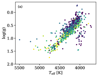
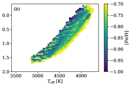
To explore differences in metallicity, we analyze the APOGEE stars in front and behind components. In addition to radial velocities, APOGEE provides stellar parameter measurements, including stellar metallicity, [Fe/H]. The APOGEE survey provides accurate and precise metallicity measurements for RGBs across the MW (see e.g., Jönsson et al. 2020), but there have been no assessments of the accuracy of metallicities derived from RSG spectra. While a detailed comparison of APOGEE RSG metallicities with optical studies is beyond the scope of this work, we use isochrones to determine if the relative metallicities of red supergiants are informative. Figure 13 shows a Kiel diagram colored by metallicity for the APOGEE RSGs (a) and the RSG isochrones described and used in Section 2.2.3 (b). APOGEE finds that the more metal-poor stars are generally cooler and that the more metal-rich stars are generally hotter at a fixed luminosity. Overall, the APOGEE stars show the same qualitative trend of metal-rich stars having higher temperatures at fixed log(g), suggesting that the APOGEE metallicities are at least useful in a relative sense.

We note that the subset of RSGs with low log(g) sitting below the distribution in Figure 13a are all bright ($G\lesssim 13\rm\,mag$) and “dusty” ($A_{K}>0.2$). These stars are present in both the front and behind components, and excluding them does not affect the analysis presented here (i.e., all observed signals persist).

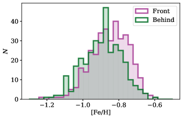
Histograms of the metallicities derived by APOGEE are shown in Figure 14. Although there is significant overlap, there is evidence that stars in the front component have higher metallicity. A Kolmogorov-Smirnoff test between the two samples rejects the null hypothesis that they were drawn from the same parent population with $p=10^{-8}$.

To check whether the observed difference in metallicity is due to a bias in observed magnitudes (e.g., is the behind component dominated by the brightest, intrinsically lowest-metallicity sources?), we compare the CMDs of the two components. We find that both components have stars spanning the full range of observed magnitudes in the RSG selection (Figure 2). The completeness in our sample at these bright magnitudes is expected to be close to 1, and therefore the difference in metallicity is not likely to be a result of observational selection.

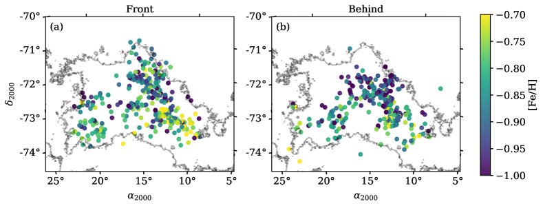
In Figure 15 we plot the spatial distribution of RSGs in the front and behind components, colored by metallicity. The majority of the highest metallicity sources are located in the SW Bar, where the majority of the dust and molecular gas content resides (Jameson et al., 2016). Interestingly, we observe that the lowest metallicity sources are in the behind component and are distributed in the Northern Bar. As a possible explanation, there are known outflows of cold Hi from this region (e.g., McClure-Griffiths et al., 2018), and thus stars which form within outflowing gas may be more metal poor than those forming with the Bar, which is a possibility for both the front and behind components.

4 Simple Model for Component Distances

In the following section, we construct a simple toy model to constrain the distances to the front and behind components based on their observed kinematics. Although the history of the LMC-SMC system is extremely complex to model, even in the latest hydrodynamical N-body simulations (Besla et al., 2012), our goal is to determine whether a simple, physically-meaningful model can explain our results in broad strokes.

We treat the two components (front and behind) as independent structures experiencing tidal effects from the LMC (evident by the gradient in $\mu_{W}$; Figure 10) as well as rotation (evident from residual $\mu_{\theta}$; Figure 11). We do not consider the bulk motion of the LMC and SMC in the model, we model all stars in the reference frame of the LMC-SMC system, and calculate the tidal force at a fixed distance to the LMC over time.

For each component, we initialize a population of stars with positions distributed normally with $\sigma=1\rm\,kpc$ in each of the $x$, $y$ and $z$ dimensions. This value was chosen to roughly model the observed distribution of stars in $X$ and $Y$, and we assume for simplicity that the systems are symmetric in $Z$. The stars are given velocities with random Gaussian amplitude and $\sigma=20\rm\,km\,s^{-1}$ in the $x$, $y$, and $z$ directions. This value was chosen based on the average standard deviation in the values of $\mu_{N}$ for both samples, converted from $\rm mas/yr$ to $\rm km/s$ assuming a distance of $62\rm\,kpc$. In the plane of the sky, the LMC is located at a distance of $d_{\rm LMC,\,sky}=20\rm\,kpc$, and has a mass of $M_{\rm LMC}=1.4\times 10^{11}\rm\,M_{\odot}$ (Erkal et al., 2019).

Figure 16: Results of the MCMC simple model fit procedure to the front (purple) and behind (green) structures. 2D histograms display the $1$, $2$ and $3\sigma$ limits of each posterior distribution. Histograms display 1D marginalized posterior PDFs of each parameter.

Next, we construct a simple prescription for the differential tidal force on the stars due to the LMC. Considering the large uncertainties in the SMC geometry, we only consider a simplistic tidal prescription (i.e., omitting the influence of the Milky Way and angular momentum effects). By integrating the tidal acceleration on the stars over a timescale $\Delta t$, and assuming the distance from the center of the system to the the LMC ($r_{\rm LMC}$) is much larger than the distance from each star to the center of mass ($r$), we can compute the velocity in the LMC direction of each star as a result of tides via:

$$v_{t,\rm LMC}(r)\approx\frac{2\,G\,M_{\rm LMC}\,r^{2}}{r_{\rm LMC}^{3}}\,\Delta t.$$ (4)

In addition to the tidal velocity, we also include a simple prescription for a rotational component ($v_{\rm rot}$) as a function of the observed coordinates,

$$v_{\rm rot}(X)=\frac{2}{\pi}\,v_{f}\arctan\left(\frac{X}{X_{f}}\right),$$ (5)

following Di Teodoro et al. (2019) for asymptotic velocity $v_{f}$ and scale radius $X_{f}$ (we assume $X_{f}=1\rm\,kpc$). Of course, this prescription assumes a particular orientation of the rotation in each system, as we do not take inclination or higher-order kinematic effects into account. We emphasize that this is out of scope for this work.

Given this simple model, we can project the resulting velocities into the three observable components, $v_{r}$, $\mu_{W}$ and $\mu_{N}$ based on the values of the three free parameters, $d_{\rm SMC}$, $\Delta t$ and $v_{f}$ and compare them with the results of Figure 10. Because we declined to correct the observations for perspective rotation, we add this effect to the model (i.e., for which we know the distance to each source), using Equation 6 of van de Ven et al. (2006), reproduced below for clarity:

$$\mu_{X}^{\rm pr} =-6.1363\times 10^{-5}\,X\,v_{r,\,\rm sys}/d_{\rm SMC}$$ (6)

$$\mu_{Y}^{\rm pr} =-6.1363\times 10^{-5}\,Y\,v_{r,\,\rm sys}/d_{\rm SMC}$$

$$v_{r}^{\rm pr} =1.3790\times 10^{-3}\,(X\,\mu_{X,\rm sys}+Y\,\mu_{Y,\rm sys})/d_{\rm SMC},$$

where $d_{\rm SMC}$ is the line of sight distance to the center of the system in our observed reference frame, and is computed from $r_{\rm LMC}$ via,

$$d_{\rm SMC}=50\,+\sqrt{r_{\rm LMC}^{2}+d_{\rm LMC,\,sky}^{2}}\rm\,kpc.$$ (7)

Figure 17: The best-fitting toy model results (black contours, denoting $1$, $2$ and $3\sigma$ limits of the model distributions) overlaid on the observed velocity components of the front and behind structures (Figure 10).

To perform the fit, we use Markov Chain Monte Carlo sampling implemented in the emcee Python package (Foreman-Mackey et al., 2013). Following Bayes’ rule, the posterior probability that our observations $\mathbf{x}$ (where $\mathbf{x}\equiv v_{r},\,\mu_{W}$) are consistent with our model, $m(\mathbf{\theta})$ (where $\mathbf{\theta}\equiv d_{\rm SMC},\,\Delta t,\,v_{f})$ is proportional to the product of the likelihood ${\rm P}(\mathbf{x}|\theta)$ and the prior ${\rm P}(\theta)$,

$${\rm P}(\mathbf{\theta}|\mathbf{x})\propto{\rm P}(\mathbf{x}|\mathbf{\theta})\,\,{\rm P}(\mathbf{\theta}).$$ (8)

Here we assume the likelihood is roughly Gaussian and independent for each of the observed quantities so that,

$${\rm P}(\mathbf{x}|\mathbf{\theta})=\prod_{x}\frac{1}{\sqrt{2\pi}\sigma_{x}}\exp{\left[-\frac{1}{2}\frac{m(\mathbf{\theta})-\mathbf{x}}{\sigma_{x}^{2}}\right]}$$ (9)

where the subscript $x$ runs between the values of $\mathbf{x}$ (i.e., $v_{r}$ and $\mu_{W}$). We assume a flat prior on each of the three free parameters, and allow them to have values in the range of $50<d_{\rm SMC}<80\rm\,kpc$ (used to compute $r_{\rm LMC}$), $\Delta t=0-1000\rm\,Myr$ and $-200<v_{f}<200\rm\,km\,s^{-1}$. We initialize the model at the same position for both samples ($d_{\rm smc},\,\Delta t,\,v_{f})=(62\rm\,kpc,\,600\rm\,Myr,\,30\rm\,km\,s^{-1})$, and sample the posterior with 1,000 walkers and 10,000 steps per parameter, excluding a burn-in phase of 1,000 steps.

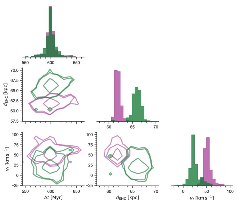
In Figure 16 we display a “corner” plot of the 2D distributions of the posterior, as well as marginalized 1D PDFs. We compute the $50^{\rm th}$ percentile of each 1D PDF and compute the uncertainties based on the $16^{\rm th}$ and $84^{\rm th}$ percentiles. These results are summarized in Table 1.

Table 1: Simple Model Fit Results

Parameter	Description	Front	Behind
$d_{\rm SMC}$ [kpc]	Line of sight distance	$61^{+2}_{-1}$	$66^{+2}_{-2}$
$\Delta t$ [Myr]	Time since tidal interaction with LMC began	$600^{+9}_{-8}$	$600^{+7}_{-6}$
$v_{f}$ [$\rm km\,s^{-1}$]	Asymptotic rotation velocity	$50^{+9}_{-5}$	$22^{+12}_{-6}$
$M_{\rm HI}$ [$M_{\odot}$]	Total Hi mass	$2.6\times 10^{8}\left(\frac{D}{61\rm\,kpc}\right)^{2}$	$2.8\times 10^{8}\left(\frac{D}{66\rm\,kpc}\right)^{2}$

Note. — Parameters derived from the MCMC fit of our simple toy model to the observed velocities of RSGs in the front and behind systems.

In Figure 17, we overlay the contours from one realization of the toy model. We observe that there is good agreement between the observations and the model contours in all panels, which is encouraging given the simplicity of the model (i.e., we did not take into account effects of the components on each other, the Milky Way, or any external effects beyond tidal acceleration from a simplistic point-mass LMC). The shape of the $\mu_{W}(X)$ distribution (middle column; Figure 17) is constrained by the $d_{\rm SMC}$ and $\Delta t$ parameters, and the shape of the $v_{r}(X)$ distributions (left column; Figure 17) is also constrained by $v_{f}$. We emphasize again that the structures were modeled independently, without prior information about their order along the line of sight (i.e., flat prior on all model parameters).

It is highly encouraging that we recover the fact that the front component is closer along the line of sight ($61^{+2}_{-1}\rm\,kpc$ versus $\sim 66^{+2}_{-2}\rm\,kpc$). In addition, our results agree with previous constraints for the distance structure to the young, star-forming components of the SMC. In particular, we agree with the analysis of Yanchulova Merica-Jones et al. (2017), who inferred the properties of dust along the line of sight by modeling the detailed structure of the red giant branch and red clump traced by UV-IR photometry of the Southwest Bar from the HST SMIDGE survey. They concluded that the dust in that region is localized to a thin layer at $\sim 62\rm\,kpc$ within a broad stellar distribution spread $\sim 10\rm\,kpc$ along the line of sight. The dust in this region is spatially coincident with molecular gas traced by CO emission, which we have shown is consistent with being located in the front component. We find consistent results for the distance to the dust in the front component of $\sim 61\rm\,kpc$.

The other two free parameters in the model, $\Delta t$ and $v_{f}$ are also consistent with expectations. The two components have statistically indistinguishable $\Delta t$, indicating that they have undergone tidal influence of the LMC for the same amount of time, which is reasonable. In the front component, $v_{f}$ is larger than in the behind component. This agrees in broad strokes with observations of $\mu_{\theta}$, which is more consistently negative in the front component than the behind. We emphasize that $v_{f}$ is extremely uncertain, as it relies on an assumed rotation axis and structure (i.e., higher-order effects such as inclination are not taken into account). Properly modeling rotation in each system requires a much more sophisticated approach, which we consider to be beyond the scope of this work. We emphasize again that this model was designed to constrain $d_{\rm SMC}$ in particular, which influences all kinematic components (rather than just $v_{r}$ in the case of $v_{f}$).

4.1 Estimating total Hi mass

Based on the results of this simple model, we estimate the total Hi masses of the two structures. The first step is to split the GASKAP-Hi cube into the front and behind structures, which requires an estimate for $\langle\Delta A_{K}\rangle$ across the full survey footprint. To estimate this, we compute the binned average of $\langle\Delta A_{K}\rangle$ in square bins 10 pixels on a side, and for pixels without a measurement, we use the average of the nearest 10 pixels with a measurement.

We then model all spectra in the SMC Hi cube with Gaussian functions using GaussPy+ (Lindner et al., 2015; Riener et al., 2019), an extremely efficient, reproducible method for spectral line decomposition. We use the simplest form of GaussPy+, which leverages the Autonomous Gaussian Decomposition algorithm to identify the positions, widths, and amplitudes of spectral lines based on their numerical derivatives, controlled by only three free parameters: smoothing scales for detecting narrow and broad components ($\alpha_{1}$ and $\alpha_{2}$) and the desired signal to noise ratio (S/N). The optimal values for $\alpha_{1}$ and $\alpha_{2}$ are chosen by running the algorithm on a training set of known decomposition, and in this case we use the helper functions from GaussPy+ to construct a training set selected from the SMC cube itself, and decompose them using an independent iterative method (for more details see Riener et al., 2019). From this process, we find that the optimal decomposition parameters are: $\alpha_{1}=1.08$ and $\alpha_{2}=4.95$ and S/N$=3$.

Figure 18: Hi column density maps of the front (left) and behind (right) components.

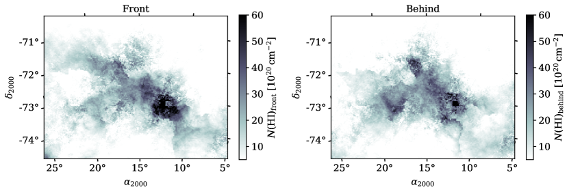
Next, for each pixel, if $\langle\Delta A_{K}\rangle<0$, we assign the emission for all fitted Gaussian components with mean velocities less than the first moment to the front component and the rest to the behind component (and vice-versa for $\langle\Delta A_{K}\rangle>0$). We assume the average distances to the front and behind structures from the simple model, $61\rm\,kpc$ and $66\rm\,kpc$ respectively, and report the Hi mass in Table 1.

Overall, the structures appear to have roughly the same Hi mass. This is not surprising, given the fact that the amplitudes of the Hi features at low and high velocities are similar throughout the system. Our estimates generally agree with previous estimates for the Hi mass of the SMC, which range from $\sim 3-6\times 10^{8}\rm\,M_{\odot}$ (Hindman, 1967; Bajaja & Loiseau, 1982; Stanimirović et al., 1999; Di Teodoro et al., 2019).

In Figure 18 we display Hi column density maps, computed in the optically-thin limit, for the front and behind components.

5 Discussion

Taken together, our results paint a picture in which the SMC is composed of two, distinct, star-forming systems which overlap along the line of sight.

At face value, this result is consistent with previous conclusions that multi-peaked Hi velocity profiles of the SMC arise due to the presence of separate sub-systems at different line of sight distances (Kerr et al., 1954; Johnson, 1961; Mathewson & Ford, 1984). The key difference is that we have shown that the two systems cannot be simply classified as having low or high velocity, as in fact the order of the velocity components along the line of sight changes as you move across the face of the SMC.

Another important difference between this work and previous analysis of the line of sight structure of the ISM is that we probe a wide range of SMC environments. For example, optical absorption lines detected towards SMC stars are typically associated with Hi at low velocities (Danforth et al., 2002; Welty et al., 2012), prompting the conclusion that gas at low velocity must be in front along the line of sight across the system. However, these studies are limited to handfuls of detections, biased towards the regions which feature the highest densities and highest optical depths. Our method allows us to probe the low-density diffuse medium of the SMC, and the smoothness of $\langle\Delta A_{K}\rangle$ (Figure 8) provides supporting evidence that we are sensitive to real changes in the column density structure in different regions.

In addition to our agreement with the only constraint for the dust geometry of the SMC in the SW Bar (Yanchulova Merica-Jones et al., 2017), we have general agreement with the picture painted by older stellar populations in the system. Cepheid variables, stars for which precise distances can be estimated, are highly-elongated (up to $\sim 20\rm\,kpc$) along the line of sight (Scowcroft et al., 2016). Although they do not show the same spatial distribution as inferred for the star-forming ISM in this work (as they are much more elongated and are generally uniformly distributed), there is clear evidence for the presence of distinct sub-structures with similar average positions along the line of sight, i.e., $\sim 60$ and $\sim 66\rm\,kpc$ (Ripepi et al., 2017; Jacyszyn-Dobrzeniecka et al., 2017). These substructures are angled across the field of view such that they overlap along the line of sight when viewed in the plane of sight, making it difficult to conduct detailed comparisons with the morphologies of the front and behind components identified here (which also overlap along the line of sight). In addition, the bimodality in distance observed in red clump stars in the East (Nidever et al., 2013; Subramanian et al., 2017; Tatton et al., 2021; Omkumar et al., 2021; Almeida et al., 2023) underscores the potential for multiple components to the SMC system. The separation between the red clump structures is larger than what we infer here ($\sim 10\rm\,kpc$), and we consider it beyond the scope of this work to determine if they are directly related (as this will require more detailed numerical modeling of the system than performed here). However, overall, we consider it to be encouraging that there is a wealth of ancillary evidence for significant substructure along the line of sight to the system.

In addition to the fact that the reservoir of cold, dense star-forming material, also displays evidence for significant substructure along the line of sight, we find that both systems identified here are actively forming stars. Taking a conservative estimate for the lifetimes of these stars to be $100\rm\,Myr$ (most are much younger; Figure 3), and a rough estimate for the relative speed of the stars with respect to the gas of $\sim 10-100\rm\,km\,s^{-1}$, the stars will travel $\sim 0.1-1\rm\,kpc$ in their lifetimes. This is only $\lesssim 20\%$ of the inferred separation of the two systems along the line of sight ($\sim 5\rm\,kpc$), which suggests the RSGs likely formed within the system they are located in today.

One possible explanation for our results is that the two systems are remnants of distinct galaxies. The difference in observed stellar metallicities, as well as the distinct difference between the molecular gas features in the two structures, suggests that they may have evolved in different ways. Although the chemical enrichment history appears similar across the SMC (Almeida et al., 2023), there is evidence for “non-uniform” enrichment in the outskirts of the system (Mucciarelli et al., 2023).

Alternatively, the front structure is the main galaxy (the “SMC Remnant”; Mathewson & Ford, 1984) and the behind structure is tidal debris resulting from the interaction with the LMC. The complex nature of the debris field surrounding the SMC, including a bifurcated bridge towards the LMC (Muller et al., 2004), and the bifurcated, trailing Stream (Putman et al., 1998; Nidever et al., 2010), support this picture. Furthermore, although in this work we have made the choice to focus on the properties of the two dominant Hi velocity features, it is clear that in some regions of the SMC there are more than two components. Although these additional components tend to have significantly smaller column density than the two main peaks, their presence highlights the possibility that additional subsystems may be identified.

One particular hypothesis of note is that the behind component is a “counter-bridge” of material pulled from the SMC as a result of its interactions with the LMC (Toomre & Toomre, 1972; Besla et al., 2012; Diaz & Bekki, 2012). According to numerical simulations of the MS, this structure is expected to sit directly behind the main body of the SMC, and if pulled from the outskirts of the system, may explain its lower observed metallicity. The caveat to this interpretation is that the two systems have roughly equal Hi mass, which is not expected in the counter-bridge model. In addition, the spatial distribution of Hi in the system indicates that the “loop” in the North East, posited to be part of the counter bridge (Muller & Bekki, 2007) is actually at the near SMC distance. However, the 3D positions and kinematics of clusters in the SMC periphery have consistent distances with the front and behind components found here, as well as being consistent with the numerical predictions of the counter bridge (Dias et al., 2022).

Ultimately, reconciling these results within the broad landscape of observational constraints for the structure of the SMC requires further work. This includes direct distance constraints to the ISM components, as well as numerical studies of the structure of the SMC in the context of the history of the full MS. However, the implications for our understanding of star formation in low-metallicity dwarf galaxies are already significant. The SMC is used as a template for the evolution of the dust-to-gas ratio with metallicity (e.g., see Clark et al., 2023). Accurately associating the diffuse, atomic gas to the metal-rich ISM is crucial for inferring this parameter, which underlies our understanding of the chemical enrichment of galaxies.

6 Summary

In this study we investigate the 3D structure of the star-forming ISM in the SMC. We compile a sample of young, massive stars from Gaia DR3 and APOGEE whose kinematics are consistent with distinct Hi velocity components observed by the high-resolution GASKAP-Hi survey. By comparing the line of sight extinction to these stars across the SMC, we find that the order of the low and high Hi velocity components changes between SMC environments. We separate the stellar sample into sub-systems, one in front along the line of sight and one behind. We find that these systems have distinct metallicity distributions, and there is evidence that the molecular gas in the SMC resides mostly in the front component. We construct a simple toy model to explain the kinematics of the two components undergoing the tidal influence of the LMC as well as rotation. We find that the two components lie $5\rm\,kpc$ from each other along the line of sight (average distances of $61$ and $66\rm\,kpc$ respectively). These results are broadly consistent with previous estimates of the line of sight structure of the SMC from diverse tracers.

7 acknowledgements

The authors acknowledge the anonymous referee, whose comments improved the clarity of the manuscript. C.E.M. acknowledges insightful conversations with Christopher Clark, Karl Gordon, Peter Scicluna, Lara Cullinane and David French during the development of this project. The authors acknowledge Interstellar Institute’s program “II6” and the Paris-Saclay University’s Institut Pascal for hosting discussions that nourished the development of the ideas behind this work. J.E.M.C acknowledges STFC studentship. E.D.T. was supported by the European Research Council (ERC) under grant agreement no. 101040751. C.F. acknowledges funding provided by the Australian Research Council (Discovery Project DP230102280), and the Australia-Germany Joint Research Cooperation Scheme (UA-DAAD).

The Australian SKA Pathfinder is part of the Australia Telescope National Facility which is managed by CSIRO. Operation of ASKAP is funded by the Australian Government with support from the National Collaborative Research Infrastructure Strategy. ASKAP uses the resources of the Pawsey Supercomputing Centre. Establishment of ASKAP, the Murchison Radioastronomy Observatory and the Pawsey Supercomputing Centre are initiatives of the Australian Government, with support from the Government of Western Australia and the Science and Industry Endowment Fund. We acknowledge the Wajarri Yamatji people as the traditional owners of the Observatory site.

This work has made use of data from the European Space Agency (ESA) mission Gaia (https://www.cosmos.esa.int/gaia), processed by the Gaia Data Processing and Analysis Consortium (DPAC, https://www.cosmos.esa.int/web/gaia/dpac/consortium). Funding for the DPAC has been provided by national institutions, in particular the institutions participating in the Gaia Multilateral Agreement.

Funding for the Sloan Digital Sky Survey IV has been provided by the Alfred P. Sloan Foundation, the U.S. Department of Energy Office of Science, and the Participating Institutions. SDSS acknowledges support and resources from the Center for High-Performance Computing at the University of Utah. The SDSS web site is www.sdss4.org.

SDSS is managed by the Astrophysical Research Consortium for the Participating Institutions of the SDSS Collaboration including the Brazilian Participation Group, the Carnegie Institution for Science, Carnegie Mellon University, Center for Astrophysics — Harvard & Smithsonian (CfA), the Chilean Participation Group, the French Participation Group, Instituto de Astrofísica de Canarias, The Johns Hopkins University, Kavli Institute for the Physics and Mathematics of the Universe (IPMU) / University of Tokyo, the Korean Participation Group, Lawrence Berkeley National Laboratory, Leibniz Institut für Astrophysik Potsdam (AIP), Max-Planck-Institut für Astronomie (MPIA Heidelberg), Max-Planck-Institut für Astrophysik (MPA Garching), Max-Planck-Institut für Extraterrestrische Physik (MPE), National Astronomical Observatories of China, New Mexico State University, New York University, University of Notre Dame, Observatório Nacional / MCTI, The Ohio State University, Pennsylvania State University, Shanghai Astronomical Observatory, United Kingdom Participation Group, Universidad Nacional Autónoma de México, University of Arizona, University of Colorado Boulder, University of Oxford, University of Portsmouth, University of Utah, University of Virginia, University of Washington, University of Wisconsin, Vanderbilt University, and Yale University.

References

- Abdurro’uf et al. (2022) Abdurro’uf, Accetta, K., Aerts, C., et al. 2022, ApJS, 259, 35, doi: 10.3847/1538-4365/ac4414
- Accurso et al. (2017) Accurso, G., Saintonge, A., Catinella, B., et al. 2017, MNRAS, 470, 4750, doi: 10.1093/mnras/stx1556
- Allende Prieto et al. (2006) Allende Prieto, C., Beers, T. C., Wilhelm, R., et al. 2006, AJ, 636, 804, doi: 10.1086/498131
- Almeida et al. (2023) Almeida, A., Majewski, S. R., Nidever, D. L., et al. 2023, arXiv e-prints, arXiv:2308.13631, doi: 10.48550/arXiv.2308.13631
- Astropy Collaboration et al. (2013) Astropy Collaboration, Robitaille, T. P., Tollerud, E. J., et al. 2013, A&A, 558, A33, doi: 10.1051/0004-6361/201322068
- Astropy Collaboration et al. (2018) Astropy Collaboration, Price-Whelan, A. M., Sipőcz, B. M., et al. 2018, AJ, 156, 123, doi: 10.3847/1538-3881/aabc4f
- Babusiaux et al. (2023) Babusiaux, C., Fabricius, C., Khanna, S., et al. 2023, A&A, 674, A32, doi: 10.1051/0004-6361/202243790
- Bajaja & Loiseau (1982) Bajaja, E., & Loiseau, N. 1982, A&AS, 48, 71
- Beaumont et al. (2015) Beaumont, C., Goodman, A., & Greenfield, P. 2015, in Astronomical Society of the Pacific Conference Series, Vol. 495, Astronomical Data Analysis Software an Systems XXIV (ADASS XXIV), ed. A. R. Taylor & E. Rosolowsky, 101
- Belokurov et al. (2016) Belokurov, V., Erkal, D., Deason, A. J., et al. 2016, MNRAS, doi: 10.1093/mnras/stw3357
- Besla et al. (2007) Besla, G., Kallivayalil, N., Hernquist, L., et al. 2007, ApJ, 668, 949, doi: 10.1086/521385
- Besla et al. (2012) —. 2012, MNRAS, 421, 2109, doi: 10.1111/j.1365-2966.2012.20466.x
- Besla et al. (2016) Besla, G., Martínez-Delgado, D., van der Marel, R. P., et al. 2016, ApJ, 825, 20, doi: 10.3847/0004-637X/825/1/20
- Blanton et al. (2017) Blanton, M. R., Bershady, M. A., Abolfathi, B., et al. 2017, AJ, 154, 28, doi: 10.3847/1538-3881/aa7567
- Bowen & Vaughan (1973) Bowen, I. S., & Vaughan, A. H. 1973, Appl. Opt., 12, 1430, doi: 10.1364/AO.12.001430
- Bressan et al. (2012) Bressan, A., Marigo, P., Girardi, L., et al. 2012, MNRAS, 427, 127, doi: 10.1111/j.1365-2966.2012.21948.x
- Cappellari & Copin (2003) Cappellari, M., & Copin, Y. 2003, MNRAS, 342, 345, doi: 10.1046/j.1365-8711.2003.06541.x
- Carrera et al. (2017) Carrera, R., Conn, B. C., Noël, N. E. D., Read, J. I., & López Sánchez, Á. R. 2017, MNRAS, 471, 4571, doi: 10.1093/mnras/stx1932
- Chen et al. (2015) Chen, Y., Bressan, A., Girardi, L., et al. 2015, MNRAS, 452, 1068, doi: 10.1093/mnras/stv1281
- Chen et al. (2014) Chen, Y., Girardi, L., Bressan, A., et al. 2014, MNRAS, 444, 2525, doi: 10.1093/mnras/stu1605
- Choi et al. (2022) Choi, Y., Olsen, K. A. G., Besla, G., et al. 2022, ApJ, 927, 153, doi: 10.3847/1538-4357/ac4e90
- Choi et al. (2018) Choi, Y., Nidever, D. L., Olsen, K., et al. 2018, ApJ, 866, 90, doi: 10.3847/1538-4357/aae083
- Clark et al. (2023) Clark, C. J. R., Roman-Duval, J. C., Gordon, K. D., et al. 2023, ApJ, 946, 42, doi: 10.3847/1538-4357/acbb66
- Cullinane et al. (2023) Cullinane, L. R., Mackey, A. D., Da Costa, G. S., Koposov, S. E., & Erkal, D. 2023, MNRAS, 518, L25, doi: 10.1093/mnrasl/slac129
- Danforth et al. (2002) Danforth, C. W., Howk, J. C., Fullerton, A. W., Blair, W. P., & Sembach, K. R. 2002, ApJS, 139, 81, doi: 10.1086/338239
- de Grijs & Bono (2015) de Grijs, R., & Bono, G. 2015, AJ, 149, 179, doi: 10.1088/0004-6256/149/6/179
- De Leo et al. (2020) De Leo, M., Carrera, R., Noël, N. E. D., et al. 2020, MNRAS, 495, 98, doi: 10.1093/mnras/staa1122
- Di Teodoro et al. (2019) Di Teodoro, E. M., McClure-Griffiths, N. M., Jameson, K. E., et al. 2019, MNRAS, 483, 392, doi: 10.1093/mnras/sty3095
- Dias et al. (2022) Dias, B., Parisi, M. C., Angelo, M., et al. 2022, MNRAS, 512, 4334, doi: 10.1093/mnras/stac259
- Diaz & Bekki (2012) Diaz, J. D., & Bekki, K. 2012, ApJ, 750, 36, doi: 10.1088/0004-637X/750/1/36
- Dobbie et al. (2014) Dobbie, P. D., Cole, A. A., Subramaniam, A., & Keller, S. 2014, Monthly Notices of the Royal Astronomical Society, 442, 1663, doi: 10.1093/mnras/stu910
- El Youssoufi et al. (2023) El Youssoufi, D., Cioni, M.-R. L., Kacharov, N., et al. 2023, MNRAS, 523, 347, doi: 10.1093/mnras/stad1339
- Erkal et al. (2019) Erkal, D., Belokurov, V., Laporte, C. F. P., et al. 2019, MNRAS, 487, 2685, doi: 10.1093/mnras/stz1371
- Evans & Howarth (2008) Evans, C. J., & Howarth, I. D. 2008, MNRAS, 386, 826, doi: 10.1111/j.1365-2966.2008.13012.x
- For et al. (2014) For, B. Q., Staveley-Smith, L., Matthews, D., & McClure-Griffiths, N. M. 2014, ApJ, 792, 43, doi: 10.1088/0004-637X/792/1/43
- For et al. (2016) For, B. Q., Staveley-Smith, L., McClure-Griffiths, N. M., Westmeier, T., & Bekki, K. 2016, MNRAS, 461, 892, doi: 10.1093/mnras/stw1364
- Foreman-Mackey et al. (2013) Foreman-Mackey, D., Hogg, D. W., Lang, D., & Goodman, J. 2013, PASP, 125, 306, doi: 10.1086/670067
- Gaia Collaboration et al. (2016) Gaia Collaboration, Prusti, T., de Bruijne, J. H. J., et al. 2016, A&A, 595, A1, doi: 10.1051/0004-6361/201629272
- Gaia Collaboration et al. (2018a) Gaia Collaboration, Helmi, A., van Leeuwen, F., et al. 2018a, A&A, 616, A12, doi: 10.1051/0004-6361/201832698
- Gaia Collaboration et al. (2018b) —. 2018b, A&A, 616, A12, doi: 10.1051/0004-6361/201832698
- Gaia Collaboration et al. (2021) Gaia Collaboration, Luri, X., Chemin, L., et al. 2021, A&A, 649, A7, doi: 10.1051/0004-6361/202039588
- Gaia Collaboration et al. (2023) Gaia Collaboration, Vallenari, A., Brown, A. G. A., et al. 2023, A&A, 674, A1, doi: 10.1051/0004-6361/202243940
- García Pérez et al. (2016) García Pérez, A. E., Allende Prieto, C., Holtzman, J. A., et al. 2016, AJ, 151, 144, doi: 10.3847/0004-6256/151/6/144
- Gerrard et al. (2023) Gerrard, I. A., Federrath, C., Pingel, N. M., et al. 2023, arXiv e-prints, arXiv:2309.10755. https://arxiv.org/abs/2309.10755
- Gordon et al. (2011) Gordon, K. D., Meixner, M., Meade, M. R., et al. 2011, AJ, 142, 102, doi: 10.1088/0004-6256/142/4/102
- Großschedl et al. (2021) Großschedl, J. E., Alves, J., Meingast, S., & Herbst-Kiss, G. 2021, A&A, 647, A91, doi: 10.1051/0004-6361/202038913
- Gunn et al. (2006) Gunn, J. E., Siegmund, W. A., Mannery, E. J., et al. 2006, AJ, 131, 2332, doi: 10.1086/500975
- Harris et al. (2020) Harris, C. R., Millman, K. J., van der Walt, S. J., et al. 2020, Nature, 585, 357, doi: 10.1038/s41586-020-2649-2
- Harris & Zaritsky (2006) Harris, J., & Zaritsky, D. 2006, AJ, 131, 2514, doi: 10.1086/500974
- Hasselquist et al. (2021) Hasselquist, S., Hayes, C. R., Lian, J., et al. 2021, ApJ, 923, 172, doi: 10.3847/1538-4357/ac25f9
- Hatzidimitriou & Hawkins (1989) Hatzidimitriou, D., & Hawkins, M. R. S. 1989, MNRAS, 241, 667, doi: 10.1093/mnras/241.4.667
- Hindman (1964) Hindman, J. V. 1964, Nature, 202, 377, doi: 10.1038/202377b0
- Hindman (1967) —. 1967, Australian Journal of Physics, 20, 147, doi: 10.1071/PH670147
- Hotan et al. (2021) Hotan, A. W., Bunton, J. D., Chippendale, A. P., et al. 2021, PASA, 38, e009, doi: 10.1017/pasa.2021.1
- Hubeny et al. (2021) Hubeny, I., Allende Prieto, C., Osorio, Y., & Lanz, T. 2021, arXiv e-prints, arXiv:2104.02829, doi: 10.48550/arXiv.2104.02829
- Hunter (2007) Hunter, J. D. 2007, Computing In Science & Engineering, 9, 90
- Israel et al. (1993) Israel, F. P., Johansson, L. E. B., Lequeux, J., et al. 1993, A&A, 276, 25
- Jacyszyn-Dobrzeniecka et al. (2016) Jacyszyn-Dobrzeniecka, A. M., Skowron, D. M., Mróz, P., et al. 2016, Acta Astron., 66, 149. https://arxiv.org/abs/1602.09141
- Jacyszyn-Dobrzeniecka et al. (2017) —. 2017, Acta Astron., 67, 1, doi: 10.32023/0001-5237/67.1.1
- Jameson et al. (2016) Jameson, K. E., Bolatto, A. D., Leroy, A. K., et al. 2016, ApJ, 825, 12, doi: 10.3847/0004-637X/825/1/12
- Johnson (1961) Johnson, H. M. 1961, PASP, 73, 20, doi: 10.1086/127613
- Jönsson et al. (2020) Jönsson, H., Holtzman, J. A., Allende Prieto, C., et al. 2020, AJ, 160, 120, doi: 10.3847/1538-3881/aba592
- Kalberla & Haud (2015) Kalberla, P. M. W., & Haud, U. 2015, A&A, 578, A78, doi: 10.1051/0004-6361/201525859
- Kalberla et al. (2010) Kalberla, P. M. W., McClure-Griffiths, N. M., Pisano, D. J., et al. 2010, A&A, 521, A17, doi: 10.1051/0004-6361/200913979
- Kallivayalil et al. (2006a) Kallivayalil, N., van der Marel, R. P., & Alcock, C. 2006a, ApJ, 652, 1213, doi: 10.1086/508014
- Kallivayalil et al. (2006b) Kallivayalil, N., van der Marel, R. P., Alcock, C., et al. 2006b, ApJ, 638, 772, doi: 10.1086/498972
- Kerr et al. (1954) Kerr, F. J., Hindman, J. F., & Robinson, B. J. 1954, Australian Journal of Physics, 7, 297, doi: 10.1071/PH540297
- Leroy et al. (2007) Leroy, A., Bolatto, A., Stanimirović, S., et al. 2007, ApJ, 658, 1027, doi: 10.1086/511150
- Lindner et al. (2015) Lindner, R. R., Vera-Ciro, C., Murray, C. E., et al. 2015, AJ, 149, 138, doi: 10.1088/0004-6256/149/4/138
- Lucchini et al. (2021) Lucchini, S., D’Onghia, E., & Fox, A. J. 2021, ApJ, 921, L36, doi: 10.3847/2041-8213/ac3338
- Ma et al. (2023) Ma, Y. K., McClure-Griffiths, N. M., Clark, S. E., et al. 2023, MNRAS, 521, 60, doi: 10.1093/mnras/stad462
- Mackey et al. (2016) Mackey, A. D., Koposov, S. E., Erkal, D., et al. 2016, MNRAS, 459, 239, doi: 10.1093/mnras/stw497
- Majewski et al. (2011) Majewski, S. R., Zasowski, G., & Nidever, D. L. 2011, ApJ, 739, 25, doi: 10.1088/0004-637X/739/1/25
- Majewski et al. (2017) Majewski, S. R., Schiavon, R. P., Frinchaboy, P. M., et al. 2017, AJ, 154, 94, doi: 10.3847/1538-3881/aa784d
- Marigo et al. (2017) Marigo, P., Girardi, L., Bressan, A., et al. 2017, ApJ, 835, 77, doi: 10.3847/1538-4357/835/1/77
- Martínez-Delgado et al. (2019) Martínez-Delgado, D., Vivas, A. K., Grebel, E. K., et al. 2019, A&A, 631, A98, doi: 10.1051/0004-6361/201936021
- Massana et al. (2022) Massana, P., Ruiz-Lara, T., Noël, N. E. D., et al. 2022, MNRAS, 513, L40, doi: 10.1093/mnrasl/slac030
- Mathewson et al. (1974) Mathewson, D. S., Cleary, M. N., & Murray, J. D. 1974, ApJ, 190, 291, doi: 10.1086/152875
- Mathewson & Ford (1984) Mathewson, D. S., & Ford, V. L. 1984, in IAU Symposium, Vol. 1983, Structure and Evolution of the Magellanic Clouds, ed. S. van den Bergh & K. S. D. de Boer, 125–136
- Mathewson et al. (1988) Mathewson, D. S., Ford, V. L., & Visvanathan, N. 1988, ApJ, 333, 617, doi: 10.1086/166772
- McClure-Griffiths et al. (2009) McClure-Griffiths, N. M., Pisano, D. J., Calabretta, M. R., et al. 2009, ApJS, 181, 398, doi: 10.1088/0067-0049/181/2/398
- McClure-Griffiths et al. (2018) McClure-Griffiths, N. M., Dénes, H., Dickey, J. M., et al. 2018, Nature Astronomy, 2, 901, doi: 10.1038/s41550-018-0608-8
- Mizuno et al. (2001) Mizuno, N., Rubio, M., Mizuno, A., et al. 2001, PASJ, 53, L45, doi: 10.1093/pasj/53.6.L45
- Mucciarelli et al. (2023) Mucciarelli, A., Minelli, A., Bellazzini, M., et al. 2023, A&A, 671, A124, doi: 10.1051/0004-6361/202245133
- Muller & Bekki (2007) Muller, E., & Bekki, K. 2007, MNRAS, 381, L11, doi: 10.1111/j.1745-3933.2007.00356.x
- Muller et al. (2004) Muller, E., Stanimirović, S., Rosolowsky, E., & Staveley-Smith, L. 2004, ApJ, 616, 845, doi: 10.1086/425154
- Muller et al. (2010) Muller, E., Ott, J., Hughes, A., et al. 2010, ApJ, 712, 1248, doi: 10.1088/0004-637X/712/2/1248
- Murai & Fujimoto (1980) Murai, T., & Fujimoto, M. 1980, PASJ, 32, 581
- Murray et al. (2019) Murray, C. E., Peek, J. E. G., Di Teodoro, E. M., et al. 2019, ApJ, 887, 267, doi: 10.3847/1538-4357/ab510f
- Nidever et al. (2010) Nidever, D. L., Majewski, S. R., Butler Burton, W., & Nigra, L. 2010, ApJ, 723, 1618, doi: 10.1088/0004-637X/723/2/1618
- Nidever et al. (2013) Nidever, D. L., Monachesi, A., Bell, E. F., et al. 2013, ApJ, 779, 145, doi: 10.1088/0004-637X/779/2/145
- Nidever et al. (2015) Nidever, D. L., Holtzman, J. A., Allende Prieto, C., et al. 2015, AJ, 150, 173, doi: 10.1088/0004-6256/150/6/173
- Nidever et al. (2020) Nidever, D. L., Hasselquist, S., Hayes, C. R., et al. 2020, ApJ, 895, 88, doi: 10.3847/1538-4357/ab7305
- Niederhofer et al. (2018) Niederhofer, F., Cioni, M. R. L., Rubele, S., et al. 2018, A&A, 613, L8, doi: 10.1051/0004-6361/201833144
- Niederhofer et al. (2021) Niederhofer, F., Cioni, M.-R. L., Rubele, S., et al. 2021, MNRAS, 502, 2859, doi: 10.1093/mnras/stab206
- Olsen et al. (2015) Olsen, K. A. G., Blum, R. D., Smart, B., et al. 2015, in Astronomical Society of the Pacific Conference Series, Vol. 491, Fifty Years of Wide Field Studies in the Southern Hemisphere: Resolved Stellar Populations of the Galactic Bulge and Magellanic Clouds, ed. S. Points & A. Kunder, 257
- Omkumar et al. (2021) Omkumar, A. O., Subramanian, S., Niederhofer, F., et al. 2021, MNRAS, 500, 2757, doi: 10.1093/mnras/staa3085
- Osorio et al. (2020) Osorio, Y., Allende Prieto, C., Hubeny, I., Mészáros, S., & Shetrone, M. 2020, A&A, 637, A80, doi: 10.1051/0004-6361/201937054
- Pardy et al. (2018) Pardy, S. A., D’Onghia, E., & Fox, A. J. 2018, ApJ, 857, 101, doi: 10.3847/1538-4357/aab95b
- Pastorelli et al. (2019) Pastorelli, G., Marigo, P., Girardi, L., et al. 2019, MNRAS, 485, 5666, doi: 10.1093/mnras/stz725
- Pastorelli et al. (2020) —. 2020, MNRAS, 498, 3283, doi: 10.1093/mnras/staa2565
- Patel et al. (2020) Patel, E., Kallivayalil, N., Garavito-Camargo, N., et al. 2020, ApJ, 893, 121, doi: 10.3847/1538-4357/ab7b75
- Peñarrubia et al. (2016) Peñarrubia, J., Gómez, F. A., Besla, G., Erkal, D., & Ma, Y.-Z. 2016, MNRAS, 456, L54, doi: 10.1093/mnrasl/slv160
- Piatek et al. (2008) Piatek, S., Pryor, C., & Olszewski, E. W. 2008, AJ, 135, 1024, doi: 10.1088/0004-6256/135/3/1024
- Pieres et al. (2017) Pieres, A., Santiago, B. X., Drlica-Wagner, A., et al. 2017, MNRAS, 468, 1349, doi: 10.1093/mnras/stx507
- Pingel et al. (2022) Pingel, N. M., Dempsey, J., McClure-Griffiths, N. M., et al. 2022, PASA, 39, e005, doi: 10.1017/pasa.2021.59
- Putman et al. (1998) Putman, M. E., Gibson, B. K., Staveley-Smith, L., et al. 1998, Nature, 394, 752, doi: 10.1038/29466
- Riener et al. (2019) Riener, M., Kainulainen, J., Henshaw, J. D., et al. 2019, A&A, 628, A78, doi: 10.1051/0004-6361/201935519
- Ripepi et al. (2017) Ripepi, V., Cioni, M.-R. L., Moretti, M. I., et al. 2017, MNRAS, 472, 808, doi: 10.1093/mnras/stx2096
- Rubio et al. (1991) Rubio, M., Garay, G., Montani, J., & Thaddeus, P. 1991, ApJ, 368, 173, doi: 10.1086/169680
- Rubio et al. (1996) Rubio, M., Lequeux, J., Boulanger, F., et al. 1996, A&AS, 118, 263
- Russell & Dopita (1992) Russell, S. C., & Dopita, M. A. 1992, ApJ, 384, 508, doi: 10.1086/170893
- Saldaño et al. (2022) Saldaño, H. P., Rubio, M., Bolatto, A. D., et al. 2022, arXiv e-prints, arXiv:2211.07792, doi: 10.48550/arXiv.2211.07792
- Santana et al. (2021) Santana, F. A., Beaton, R. L., Covey, K. R., et al. 2021, AJ, 162, 303, doi: 10.3847/1538-3881/ac2cbc
- Schruba et al. (2012) Schruba, A., Leroy, A. K., Walter, F., et al. 2012, AJ, 143, 138, doi: 10.1088/0004-6256/143/6/138
- Scowcroft et al. (2016) Scowcroft, V., Freedman, W. L., Madore, B. F., et al. 2016, ApJ, 816, 49, doi: 10.3847/0004-637X/816/2/49
- Skrutskie et al. (2006) Skrutskie, M. F., Cutri, R. M., Stiening, R., et al. 2006, AJ, 131, 1163, doi: 10.1086/498708
- Stanimirović et al. (1999) Stanimirović, S., Staveley-Smith, L., Dickey, J. M., Sault, R. J., & Snowden, S. L. 1999, MNRAS, 302, 417, doi: 10.1046/j.1365-8711.1999.02013.x
- Stanimirović et al. (2004) Stanimirović, S., Staveley-Smith, L., & Jones, P. A. 2004, ApJ, 604, 176, doi: 10.1086/381869
- Staveley-Smith et al. (1997) Staveley-Smith, L., Sault, R. J., Hatzidimitriou, D., Kesteven, M. J., & McConnell, D. 1997, MNRAS, 289, 225, doi: 10.1093/mnras/289.2.225
- Subramanian & Subramaniam (2012) Subramanian, S., & Subramaniam, A. 2012, ApJ, 744, 128, doi: 10.1088/0004-637X/744/2/128
- Subramanian et al. (2017) Subramanian, S., Rubele, S., Sun, N.-C., et al. 2017, MNRAS, 467, 2980, doi: 10.1093/mnras/stx205
- Tang et al. (2014) Tang, J., Bressan, A., Rosenfield, P., et al. 2014, MNRAS, 445, 4287, doi: 10.1093/mnras/stu2029
- Tatton et al. (2021) Tatton, B. L., van Loon, J. T., Cioni, M. R. L., et al. 2021, MNRAS, 504, 2983, doi: 10.1093/mnras/staa3857
- Tokuda et al. (2021) Tokuda, K., Kondo, H., Ohno, T., et al. 2021, ApJ, 922, 171, doi: 10.3847/1538-4357/ac1ff4
- Toomre & Toomre (1972) Toomre, A., & Toomre, J. 1972, ApJ, 178, 623, doi: 10.1086/151823
- van de Ven et al. (2006) van de Ven, G., van den Bosch, R. C. E., Verolme, E. K., & de Zeeuw, P. T. 2006, A&A, 445, 513, doi: 10.1051/0004-6361:20053061
- van der Marel & Kallivayalil (2014) van der Marel, R. P., & Kallivayalil, N. 2014, ApJ, 781, 121, doi: 10.1088/0004-637X/781/2/121
- Vasiliev (2024) Vasiliev, E. 2024, MNRAS, 527, 437, doi: 10.1093/mnras/stad2612
- Virtanen et al. (2020) Virtanen, P., Gommers, R., Oliphant, T. E., et al. 2020, Nature Methods, 17, 261, doi: https://doi.org/10.1038/s41592-019-0686-2
- Wannier et al. (1972) Wannier, P., Wrixon, G. T., & Wilson, R. W. 1972, A&A, 18, 224
- Welty et al. (2012) Welty, D. E., Xue, R., & Wong, T. 2012, ApJ, 745, 173, doi: 10.1088/0004-637X/745/2/173
- Wilson et al. (2019) Wilson, J. C., Hearty, F. R., Skrutskie, M. F., et al. 2019, PASP, 131, 055001, doi: 10.1088/1538-3873/ab0075
- Yanchulova Merica-Jones et al. (2017) Yanchulova Merica-Jones, P., Sandstrom, K. M., Johnson, L. C., et al. 2017, ApJ, 847, 102, doi: 10.3847/1538-4357/aa8a67
- Zamora et al. (2015) Zamora, O., García-Hernández, D. A., Allende Prieto, C., et al. 2015, AJ, 149, 181, doi: 10.1088/0004-6256/149/6/181
- Zasowski et al. (2017) Zasowski, G., Cohen, R. E., Chojnowski, S. D., et al. 2017, AJ, 154, 198, doi: 10.3847/1538-3881/aa8df9
- Zhang et al. (2023) Zhang, X., Green, G. M., & Rix, H.-W. 2023, arXiv e-prints, arXiv:2303.03420, doi: 10.48550/arXiv.2303.03420
- Zivick et al. (2021) Zivick, P., Kallivayalil, N., & van der Marel, R. P. 2021, ApJ, 910, 36, doi: 10.3847/1538-4357/abe1bb
- Zivick et al. (2018) Zivick, P., Kallivayalil, N., van der Marel, R. P., et al. 2018, ApJ, 864, 55, doi: 10.3847/1538-4357/aad4b0
- Zivick et al. (2019) Zivick, P., Kallivayalil, N., Besla, G., et al. 2019, ApJ, 874, 78, doi: 10.3847/1538-4357/ab0554