Robust Functional Principal Component Analysis for Non-Euclidean Random Objects

Abstract

Functional data analysis offers a diverse toolkit of statistical methods tailored for analyzing samples of real-valued random functions. Recently, samples of time-varying random objects, such as time-varying networks, have been increasingly encountered in modern data analysis. These data structures represent elements within general metric spaces that lack local or global linear structures, rendering traditional functional data analysis methods inapplicable. Moreover, the existing methodology for time-varying random objects does not work well in the presence of outlying objects. In this paper, we propose a robust method for analysing time-varying random objects. Our method employs pointwise Fréchet medians and then constructs pointwise distance trajectories between the individual time courses and the sample Fréchet medians. This representation effectively transforms time-varying objects into functional data. A novel robust approach to functional principal component analysis based on a Winsorized U-statistic estimator of the covariance structure is introduced. The proposed robust analysis of these distance trajectories is able to identify key features of time-varying objects and is useful for downstream analysis. To illustrate the efficacy of our approach, numerical studies focusing on dynamic networks are conducted. The results indicate that the proposed method exhibits good all-round performance and surpasses the existing approach in terms of robustness, showcasing its superior performance in handling time-varying objects data.

Keywords: dynamic network, Fréchet median trajectory, metric space, U-statistic, Winsorize

1 Introduction

1.1 Background

In the era of big data, it is common to observe complex data on a time grid, important examples being dynamic traffic networks, time-evolving social networks and functional Magnetic Resonance Imaging; see e.g. Worsley et al., (2002) and Kolar et al., (2010)). While such time-varying data have similarities with functional data, the observations at each time point are neither scalars nor vectors as in classical functional data analysis, but instead take values in a general metric space. In general metric spaces, vector space operations such as addition, scalar multiplication, or inner products are not defined, posing a significant challenge to traditional analysis methods.

For the analysis of non-Euclidean data, numerous works have concentrated on smooth Riemannian manifolds, typically exploiting their local Euclidean properties; see Schiratti et al., (2015), Dai and Müller, (2018), Dai et al., (2021) and Shao et al., (2022). As these approaches predominantly focus on smooth metric spaces, they are not applicable for the analysis of data objects in more general metric spaces that do not have a natural Riemannian geometry. This limitation has sparked the development of novel approaches proposed by Dubey and Müller, (2020, 2021). The approach considered in the latter paper, referred to below as Dubey and Müller’s method, focuses on the squared distance of time-varying random objects from the mean trajectory. By using these distance trajectories, Dubey and Müller’s method converts time-varying random objects into functional data, which gives access to the techniques of functional data analysis. This approach to the analysis of distance trajectories has unveiled compelling insights into the behavior of time-varying random objects across various applications. Nevertheless, a serious drawback of Dubey and Müller’s method is that it can be highly sensitive to atypical curves, i.e., outlying time-varying random objects.

For a broad and general account of the relatively new and fast-developing field of object data analysis, see the monograph Marron and Dryden, (2021).

1.2 Contributions of the paper

Our goal in this paper is to provide a novel robust methodology for analyzing time-varying random objects. Our method first constructs distance trajectories from the individual sample functions to the Fréchet median trajectory which consists of the pointwise Fréchet medians. These distance trajectories, which we refer to as Fréchet median distance trajectories, are different from the Fréchet variance trajectories in Dubey and Müller’s method, in that we measure the distance from the individual sample functions to the Fréchet median function, whereas the Dubey and Muller method works with the pointwise squared distances from the individual sample functions to the sample Fréchet mean function. We then develop a robust functional principal component method for the Fréchet median distance trajectories of which a key ingredient is a robust method for estimating the relevant autocovariance operator, using a suitable Winsorized $U$-statistic.

We briefly explain how our proposed procedure for robust autocovariance operator estimation goes beyond existing approaches. Robust principal component analysis approaches for Euclidean data using spatial sign covariance and spherical principal component approaches for functional data have been studied in Marden, (1999), Visuri et al., (2000) and Gervini, (2008). However, these approaches require that data are symmetrically distributed and, in addition, there is scope for improving their performance with respect to robustness. Taskinen et al., (2012), Han and Liu, (2018), Zhong et al., (2022) and Wang et al., (2023) utilize pairwise covariance to waive symmetry requirements but these methods have limited performance with respect to robustness. Raymaekers and Rousseeuw, (2019) and Leyder et al., (2023) extend spatial sign covariance to achieve better robustness in Euclidean cases but they are still reliant on a symmetry assumption. Our proposed method does not require that data are symmetric and is expected to outperform spherical principal component approaches with respect to robustness. Our approach has the potential to inspire novel types of principal component analysis in Euclidean, Hilbert space and object data settings.

There exist two major obstacles in working with Fréchet median distance trajectories, which make it difficult to directly apply functional data analysis. These are (i) the fact that distance trajectories are nonnegative, which suggests that a symmetry assumption will not be reasonable; and (ii) the dependence induced by using a common sample-based function, the sample Fréchet median, from which to calculate distances. We briefly explain how we deal with these two challenges. Regarding (i), various robust methodologies have been proposed such as the spherical principal component approach of Locantore et al., (1999) and Gervini, (2008) and the projection-pursuit approach of Bali and Boente, (2009). However, most of the robust functional principal component methods are reliant on a symmetry assumption, which does not align with the asymmetric nature of the nonnegative-Fréchet median distance trajectories. As already mentioned, our approach side-steps the need for symmetry requirements.

Regarding (ii), the dependency challenge arises from the unknown population Fréchet median trajectory and a sample version of the Fréchet median trajectory needs to be estimated from the data. The distance trajectories which are used for the analysis are then the distances of the individual time courses from the sample Fréchet median trajectory. This induces dependence between the Fréchet median distance trajectories. By introducing a Winsorized U-statistic into the pairwise autocovariance operator, we are able to overcome this problem and to establish desirable asymptotic properties of the eigenfunction estimation, including rates of convergence.

Numerical studies in this paper showcase that our approach to functional principal components analysis using Fréchet median distance trajectories produces robust estimation of eigenfunctions while Dubey and Müller’s method is sensitive to outliers. Moreover, the methodology introduced in this paper accentuates the importance of drawing conclusions about time-course behaviors based on their distances from the Fréchet median trajectory. The pointwise Fréchet medians provide a robust representative for the most central point for a sample object functions and the Fréchet median distance trajectories carry information about the deviations of individual trajectories from the central trajectory. As demonstrated in the numerical studies, the proposed robust method is useful for cluster analysis of time-varying object data and also for the detection of outlying objects.

2 Preliminaries and Methodologies

Consider an object space $(\Omega,d)$ that is a totally bounded separable metric space, defined e.g. in van der Vaart and Wellner, (1996), and an $\Omega$-valued stochastic process $\{X(t)\}_{t\in[0,1]}$. Assume that we observe a sample of random object trajectories $X_{1}(t),\ldots,X_{n}(t)$ which are independently and identically distributed (IID) copies of the random process $X(t)$. Partly motivated by Dubey and Müller’s method, for each subject-specific trajectory $X_{i}(t)$, we aim to quantify its deviation from a baseline object function which, for robustness purposes, is chosen to be the Fréchet median function. For given $t\in[0,1]$, the population and sample Fréchet median trajectories at $t$ are defined as

$$\mu_{\rm GM}(t)=\operatorname*{arg\,min}_{\omega\in\Omega}E[d(X(t),\omega)],~{}\hat{\mu}_{\rm GM}(t)=\operatorname*{arg\,min}_{\omega\in\Omega}\frac{1}{n}\sum_{i=1}^{n}d(X_{i}(t),\omega),$$ (2.1)

respectively. Here we assume that for all $t\in[0,1]$ these minimizers exist and are unique. Discussions of the existence and the uniqueness of the Fréchet median can be found in Sturm, (2003) and Ahidar-Coutrix et al., (2020). Our target functions for downstream analysis will be

$$V_{i}(t)=d(X_{i}(t),\mu_{\rm GM}(t)),t\in[0,1],$$

which correspond to the pointwise distance functions of the subject trajectories $X_{i}$ from the population Fréchet median trajectories. Our target functions effectively transform time-varying random objects into functional data, and functional principal component analysis is a typical dimension reduction step in functional data analysis, which is based on using the eigenfunctions of the autocovariance operator of the observations. The population Fréchet covariance function $C$ for a typical $V(t)$ is

$$C(s,t)=E[V(s)V(t)]-E[V(s)]E[V(t)],$$ (2.2)

where $V(t)=d(X(t),\mu_{\rm GM}(t)),t\in[0,1]$ is the population Fréchet median distance trajectories.

The eigenvalues of the autocovariance operator are nonnegative as the covariance surface is symmetric and nonnegative definite. By Mercer’s theorem (Hsing and Eubank, 2015),

$$C(s,t)=\sum_{j=1}^{\infty}\lambda_{j}(C)\phi_{j}(s)\phi_{j}(t),s,t\in[0,1]$$ (2.3)

with uniform convergence, where the $\lambda_{j}(C)$ are the eigenvalues of the covariance operator $C$, ordered in decreasing order, and $\phi_{j}(\cdot)$ are the corresponding orthonormal eigenfunctions. Based on the decomposition of the autocovariance operator, we have the Karhunen-Loève expansion of the Fréchet median distance trajectories,

$$V(t)=\nu(t)+\sum_{j=1}^{\infty}B_{j}\lambda_{j}^{1/2}(C)\phi_{j}(t),$$

with $L^{2}$ convergence. Here $\nu$ is the mean function of the subject-wise Fréchet median distance functions, the $B_{j}$ are uncorrelated across $j$ with $E(B_{j})=0$ and ${\rm var}(B_{ij})=1$. Note that $B_{j}\lambda_{j}^{1/2}(C)=\int(V(t)-\nu(t))\phi_{j}(t)dt$ are the functional principal components.

To achieve robustness, we consider an autocovariance operator using a Winsorized pairwise U-statistic which is given by

$$C_{\rm WPU}(s,t)=E\left[\xi^{2}(\|V(\cdot)-\widetilde{V}(\cdot)\|)\{V(s)-\widetilde{V}(s)\}\{V(t)-\widetilde{V}(t)\}\right],$$ (2.4)

where $\|\cdot\|$ is the Hilbert norm, $\xi(\cdot):[0,\infty)\to(0,\infty)$ is a Winsorized radius function given by

$$\xi(r)=\begin{cases}1,&r\leq Q\\ Q/r&r>Q,\end{cases}$$

with $Q$ being a cutoff point depending on $\|V(\cdot)-\widetilde{V}(\cdot)\|$, and $\widetilde{V}(\cdot)$ is a independent copy of $V(\cdot)$. It can be readily seen that the radius function $\xi(\cdot)$ is bounded, which will ensure the desirable asymptotic properties of the robust functional principal component analysis eigenfunction estimation. By utilizing the Winsorized pairwise U-statistic, the autocovariance operator (2.4) will have the same set of eigenfunctions with the same order of eigenvalues as those of the regular covariance function (2.2), which is discussed in Theorem 3. For convenience purposes, we let $\phi_{j}(\cdot)$ be the eigenfunction of $C_{\rm WPU}$, corresponding to the $j$-th eigenvalues.

3 Theoretical Properties

3.1 Preliminaries

We now develop theoretical frameworks of estimation theory and analysis of robustness. In §3.2, we establish asymptotic properties of the empirical estimators of the population targets as described in §2. In §3.3, we derive theoretical results of robustness, including the influence functions of eigenfunctions and the upper breakdown point of the proposed robust autocovariance estimator. Assumptions needed for our estimation theory and analysis of robustness are presented and discussed in the Appendix. All proofs in this article are given in the supplementary material.

3.2 Estimation

If the population Fréchet median trajectory $\mu_{\rm GM}$ is known, the oracle estimator of the Winsorized autocovariance surface $C_{\rm WPU}$ is

$$\widetilde{C}_{\rm WPU}(s,t)=\frac{2}{n(n-1)}\sum_{1\leq j<k\leq n}\xi^{2}(d_{jk})\{V_{j}(s)-V_{k}(s)\}\{V_{j}(t)-V_{k}(t)\},$$ (3.1)

where $d_{jk}=\|V_{j}(\cdot)-V_{k}(\cdot)\|$. Under Assumption 3 in the Appendix, standard asymptotic theory from the U-process (Arcones and Giné, 1993) that this estimator has desirable asymptotic properties and converges to the true Winsorized autocovariance surface $C_{\rm WPU}$.

However, the population Fréchet median trajectory $\mu_{\rm GM}$ is unknown in practice, we need to use the sample Fréchet median $\hat{\mu}_{\rm GM}$ to replace it in (3.1). Define $\hat{d}_{jk}=\|\hat{V}_{j}(\cdot)-\hat{V}_{k}(\cdot)\|$, the sample version of $C_{\rm WPU}$ is

$$\widehat{C}_{\rm WPU}(s,t)=\frac{2}{n(n-1)}\sum_{1\leq j<k\leq n}\xi^{2}(\hat{d}_{jk})\{\hat{V}_{j}(s)-\hat{V}_{k}(s)\}\{\hat{V}_{j}(t)-\hat{V}_{k}(t)\}.$$

A key step to derive the limiting behavior of $\widehat{C}_{\rm WPU}$ given in Theorem 1 below is to show that $\widehat{C}_{\rm WPU}$ is asymptotically close to the oracle estimator $\widetilde{C}_{\rm WPU}$.

Theorem 1.

For a function $\omega(\cdot)\in\mathcal{H}$, define $U(\omega(\cdot),s,t)=E[f_{\omega(\cdot),s,t}(X(\cdot),\widetilde{X}(\cdot))]$, where $\widetilde{X}$ is an IID copy of $X$ and

$$f_{\omega(\cdot),s,t}(X(\cdot),\widetilde{X}(\cdot))$$

$$= \left[d(\omega(s),X(s))-d(\omega(s),\widetilde{X}(s))\right]\left[d(\omega(t),X(t))-d(\omega(t),\widetilde{X}(t))\right]$$

$$\times\xi^{2}\left(\|d(\omega(\cdot),X(\cdot))-d(\omega(\cdot),\widetilde{X}(\cdot))\|\right)$$

$$-\left[d(\mu_{\rm GM}(s),X(s))-d(\mu_{\rm GM}(s),\widetilde{X}(s))\right]\left[d(\mu_{\rm GM}(t),X(t))-d(\mu_{\rm GM}(t),\widetilde{X}(t))\right]$$

$$\times\xi^{2}\left(\|d(\mu_{\rm GM},X(\cdot))-d(\mu_{\rm GM},\widetilde{X}(\cdot))\|\right).$$

Let $U_{\hat{\mu}_{GM}}(s,t)=\left.U(\omega(\cdot),s,t)\right|_{\omega(\cdot)=\hat{\mu}_{GM}}$, that is, $U_{\hat{\mu}_{GM}}(s,t)$ is obtained by letting $\omega(\cdot)=\hat{\mu}_{GM}$ in $U(\omega(\cdot),s,t)$. Under Assumptions 1-4 in the Appendix, the sequence of stochastic processes

$$U_{n}(s,t)=\sqrt{n}\left(\hat{C}_{\rm WPU}(s,t)-C_{\rm WPU}(s,t)-U_{\hat{\mu}_{GM}}(s,t)\right)$$

converges weakly to a Gaussian process with mean zero and covariance function

$$R_{(s_{1},t_{1}),(s_{2},t_{2})}={\rm Cov}\left(f_{s_{1},t_{1}}(X(\cdot),\widetilde{X}(\cdot)),f_{s_{2},t_{2}}(X(\cdot),\widetilde{X}(\cdot))\right),$$

where

$$f_{s,t}(x(\cdot),y(\cdot))= \left[d(\mu_{\rm GM}(s),x(s))-d(\mu_{\rm GM}(s),y(s))\right]\left[d(\mu_{\rm GM}(t),x(t))-d(\mu_{\rm GM}(t),y(t))\right]$$

$$\times\xi^{2}\left(\|d(\mu_{\rm GM},x(\cdot))-d(\mu_{\rm GM},y(\cdot))\|\right).$$

Theorem 1 shows that $U_{\hat{\mu}_{GM}}(s,t)$ actually affects the convergence rate of the proposed estimator. The asymptotic behaviour of $U_{\hat{\mu}_{GM}}(s,t)$ is given in our next result, which determines the uniform convergence and rates of convergence of $\sup_{t\in[0,1]}\left|\hat{\phi}_{j}(t)-\phi_{j}(t)\right|$, where $\hat{\phi}_{j}(t)$ is the $j$-th empirical eigenfunctions of the $\widehat{C}_{\rm WPU}$.

Theorem 2.

Under Assumptions 1-5 in the Appendix with $\delta_{j}$ defined in Assumption 5, we have

$$\sup_{s,t\in[0,1]}\left|U_{\hat{\mu}_{GM}}(s,t)\right|=O_{p}\left(n^{-1/2}\right),$$

and

$$\sup_{t\in[0,1]}\left|\hat{\phi}_{j}(t)-\phi_{j}(t)\right|=O_{p}\left(\delta_{j}^{-1}n^{-1/2}\right),$$

if $\beta=2$ with $\beta$ defined in Assumption 2 in the Appendix. Otherwise,

$$\sup_{s,t\in[0,1]}\left|U_{\hat{\mu}_{GM}}(s,t)\right|=O_{p}\left(\max\left\{n^{-1/2},\left(n^{-2}\log(n)\right)^{1/\{4(\beta-1)\}}\right\}\right),$$

and

$$\sup_{t\in[0,1]}\left|\hat{\phi}_{j}(t)-\phi_{j}(t)\right|=O_{p}\left(\max\left\{n^{-1/2},\left(n^{-2}\log(n)\right)^{1/\{4(\beta-1)\}}\right\}\right).$$

It is worth noting that object spaces that satisfy Assumption 2 in the Appendix with $\beta=2$ include graph Laplacians of networks with the Frobenius metric, univariate probability distributions with the 2-Wasserstein metric and correlation matrices of a fixed dimension with the Frobenius metric (Petersen and Müller, 2019; Dubey and Müller, 2021).

3.3 Analysis of Robustness

The first result in this subsection shows that, the Winsorized autocovariance operator (2.4) has the same set of eigenfunctions as those of the regular autocovariance function (2.2). In addition, although the eigenvalues of the Winsorized autocovariance operator are generally different from those of the regular autocovariance function, they remain of the same order under an additional distributional assumption.

Theorem 3.

Under Assumption 6 in the Appendix, the Winsorized autocovariance function (2.4) admits the following decomposition

$$C_{\rm WPU}(s,t)=\sum_{j=1}^{\infty}\lambda_{j}(C_{\rm WPU})\phi_{j}(s)\phi_{j}(t),s,t\in[0,1],$$ (3.2)

where for any $j$ such that $\lambda_{j}(C)>0$,

$$\lambda_{j}(C_{\rm WPU})=\lambda_{j}(C)E\left[Z_{j}^{2}\xi\left(\sum_{l=1}^{\infty}Z_{l}^{2}\lambda_{l}(C)\right)\right],$$

with $Z_{j}=\langle V-\widetilde{V},\phi_{j}\rangle/\lambda_{j}^{1/2}(C)$ and $\langle\cdot,\cdot\rangle$ is the inner product operator in the relevant Hilbert space. If $Z_{j}$, $j=1,2,\ldots$, are further assumed to be exchangeable, then for any positive integers $j,k$, $\lambda_{j}(C)\leq\lambda_{k}(C)$ implies that $\lambda_{j}(C_{\rm WPU})\leq\lambda_{k}(C_{\rm WPU})$.

Decomposition (3.2) in Theorem 3 provides the theoretical basis for using the sample version of $C_{\rm WPU}$ as a robust estimator of the eigenfunctions of $C$ defined in (2.2) and (2.3).

For analysis of robustness, given $\varepsilon\in[0,1)$, consider the $\varepsilon$-contamination neighbourhood of a probability measure $P_{0}$,

$$\mathcal{N}_{\varepsilon}(P_{0})=\{(1-\varepsilon)P_{0}+\varepsilon Q:Q~{}{\rm a~{}probability~{}measure~{}on}~{}L^{2}([0,1])\}.$$

Let $\Phi_{k}(P)$ be the $k$-th principal component of a random process with distribution $P$. One of the measures of robustness is the influence function (Huber, 2004), which measures the sensitivity of an estimator to clustered outliers. The influence function is defined as ${\rm IF}_{\Phi_{k}}(z(\cdot))=\lim_{\varepsilon\to 0}\varepsilon^{-1}\{\Phi_{k}(P_{\varepsilon,z(\cdot)})-\Phi_{k}(P_{0})\}$, where $P_{\varepsilon,z(\cdot)}=(1-\varepsilon)P_{0}+\varepsilon\delta_{z(\cdot)}$ and $\delta_{z(\cdot)}$ is the point-mass probability at $z(\cdot)\in L^{2}([0,1])$. The next theorem gives the influence function of $\Phi_{k}$.

Theorem 4.

Suppose that Assumption 6 holds. When $z(\cdot)=\mu_{\rm GM}$,

$${\rm IF}_{\Phi_{k}}(z(\cdot))=0.$$

When $z(\cdot)\neq\mu_{\rm GM}$,

$${\rm IF}_{\Phi_{k}}(z(\cdot))=2\sum_{j\neq k}\left(\lambda_{k}(C_{\rm WPU})-\lambda_{j}(C_{\rm WPU})\right)^{-1}E_{P_{0}}[\zeta_{j}(z(\cdot))\zeta_{k}(z(\cdot))]\phi_{j},$$

where

$$\zeta_{j}(z(\cdot))=\left\langle d(X(\cdot),\mu_{\rm GM})-d(z(\cdot),\mu_{\rm GM}),\phi_{j}\right\rangle\xi\left(\|d(X(\cdot),\mu_{\rm GM})-d(z(\cdot),\mu_{\rm GM})\|\right).$$

Moreover, the gross-error sensitivity is

$$\gamma_{\Phi_{k}}^{*}=\sup\left\{\|{\rm IF}_{\Phi_{k}}(z(\cdot))\|:z(\cdot)\in L^{2}([0,1])\right\}=\{p_{1}+Q(1-p_{1})\}/c_{k},$$

where $c_{k}=\min\{\lambda_{k}(C_{\rm WPU}),\{\min|\lambda_{k}(C_{\rm WPU})-\lambda_{j}(C_{\rm WPU})|:j=1,\ldots,p,j\neq k\}\}$ and $p_{1}=P\Big{(}\|d(X(\cdot),\mu_{\rm GM})-d(z(\cdot),\mu_{\rm GM})\|>Q\Big{)}$.

This theorem indicates the influence function of $\Phi_{k}$ depends strongly on the eigenvalue spacings. If we have a sequence of distinct eigenvalues that means Assumption 5 in the Appendix holds, the principal components will be robust as the gross-error sensitivity is bounded.

Note that the autocovariance operator $C_{\rm WPU}$ involves a cutoff point $Q$ and the choice of $Q$ will affect the breakdown point of $C_{\rm WPU}$. Define $\Delta=\|V(\cdot)-\widetilde{V}(\cdot)\|$. The upper breakdown of $C_{\rm WPU}$ operator is given by the following theorem.

Theorem 5.

Suppose that $\Delta=\|V(\cdot)-\widetilde{V}(\cdot)\|$ has a cumulative distribution function $G$ with $\alpha$-quantile $Q_{\alpha}$, i.e., $Q_{\alpha}=\min\{q:P(\Delta\leq q)\geq\alpha\}$. If we choose the cutoff point $Q=Q_{\psi}$, then the upper breakdown of $C_{\rm WPU}$ is $(1-\psi)^{1/2}$. That is, $n(1-\psi)^{1/2}$ is the smallest number of bad observations that can force $C_{\rm WPU}$ to breakdown, in the sense of the order of eigenvalues of $C_{\rm WPU}$.

In practice, we do not know $Q_{\psi}$, but it can be consistently estimated as follows in finite samples. Given a sample $\hat{V}_{1}(\cdot),\ldots,\hat{V}_{n}(\cdot)$, define

$$\Delta_{ij}=\|\hat{V}_{i}(\cdot)-\hat{V}_{j}(\cdot)\|,~{}1\leq i<j\leq n.$$

Define $N=n(n-1)/2$ and write

$$\Delta_{(1)}\leq\Delta_{(2)}\leq\ldots\leq\Delta_{(N)}$$

for the ordered values of $\{\Delta_{ij}\}$. Then $\hat{Q}$, a consistent estimator of $Q_{\psi}$, is given by $\hat{Q}=\Delta_{(m(\psi))}$, where $m(\psi)=n\psi(n-1)/2$.

4 Case Study

The New York City Citi Bike sharing system provides historical bike trip data publicly, available at https://citibikenyc.com/system-data. This data set records trip start and end times, along with start and end locations, at a second-resolution level, encompassing trips between bike stations in New York City.

We focus on the trips records between January 2017 to June 2020. Our study delves into the daily evolution of bike rides between various bike stations, offering insights into the Citi Bike sharing system and transportation patterns in the city. We’ve focused on the top 90 popular stations and divided each day into 20-minute intervals. Within each 20 minute interval, a network is constructed comprising 90 nodes (corresponding to the selected bike stations). Edge weights represent the number of recorded bike trips between the pairs of stations, forming the time-varying network for each of the 1273 observed days in the years 2017 to 2020. The time points where the network is sampled over the course of each day were chosen as the midpoints of the 20 minute intervals of a day. The observations at each time point correspond to a 90 dimensional graph Laplacian that characterizes the network between the 90 bike stations of interest for that particular 20 minute interval. The graph Laplacians $L$ for a network with $p$ nodes is obtained via $L=D-A$, where $A$ is the $p\times p$ adjacency matrix with the $(i,j)$-th entry $a_{ij}$ representing the edge weight between nodes $i$ and $j$, and $D$ is the degree matrix, the off-diagonal entries of which are zero, with diagonal entries $d_{ii}=\sum_{j=1}^{p}a_{ij}$. The graph Laplacian determines the simple network uniquely.

In the present case study, the distance between graph Laplacians is calculated using the Frobenious norm, an extrinsic metric. The sample Fréchet median at a particular time point is chosen to minimize the relevant sum of Frobenious distances. We then obtained the Fréchet median distance trajectories for each day, which for a given day and time point correspond to the Frobenius distance between the graph Laplacian and the Fréchet median graph Laplacian. The resulting robust estimator of the autocovariance function was applied to these 1273 Fréchet median distance trajectories. The mean Fréchet median distance trajectory of the daily graph Laplacians for the Citi Bike trip networks as a function of the time within the day, which quantifies the average deviation from the median trajectory, is shown in the left plot of Fig. 1. The peaks are at 8 am with elevated mean variation between between 6 am to 10 am and at 6 pm with elevated levels between 4 pm to 7 pm, which reflect morning and late afternoon and early evening commuting surges, where the network variation is seen to be highest.

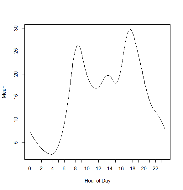
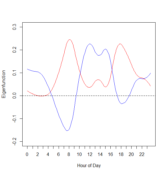
Figure 1: Sample mean function (left plot) and eigenfunctions for the robust functional component analysis (right plot) of the distance trajectories at 20 minute intervals of graph Laplacians of daily Citi Bike trip networks in New York City. In the right plot, the red line corresponds to the first eigenfunction, which explains 59.25% of variability in the trajectories and the blue line to the second eigenfunction, which explains 13.54% of the variability.

The first two eigenfunctions of the robust autocovariance function estimator, elucidated in the right plot of Fig. 1, explain about 72.79% of the variation in the trajectories. The first eigenfunction reflects increased variability around the peaks of the Fréchet median function that is shown in Fig. 1, aligning with commutor rush hours.

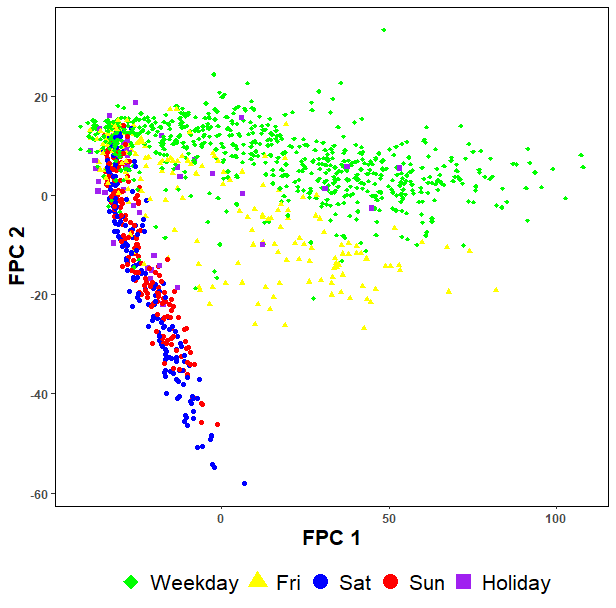
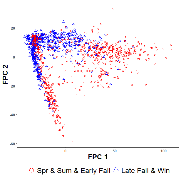
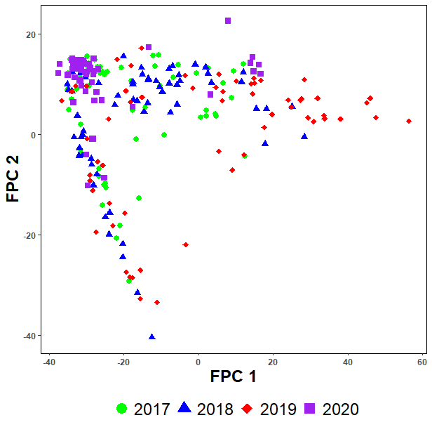
Figure 2: Pairwise plots of the first two functional principal component scores, distinguished by day of the week (left plot), by season (middle plot), and by year (right plot).

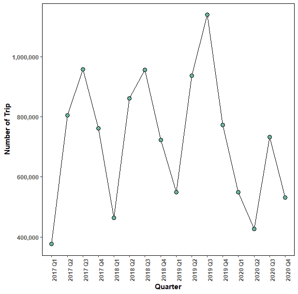
Figure S9: Plot of the number of trips between selected stations in New York City from 2017 to 2020.

Analyzing the functional principal component scores of the daily Fréchet median distance trajectories along the first and second eigenfunctions, Fig. 2 reveals three interesting patterns in the daily Fréchet median distance trajectories. First, we observe that weekdays and weekends form distinct clusters, which can be seen in the left plot of Fig. 2. Second, seasonal differences can impact bike sharing patterns. In the middle plot of Fig. 2, we display first versus second principal component scores, differentiated according to two broad seasonal groups. Spring, summer and early fall includes months from April to October that exhibit greater variability than the late fall and winter months of November to March. By analyzing the number of trips in these two seasonal groups which can be found in Fig. S9 in the supplementary material, we find that the larger number of trips will result in larger variability. Similar pattern can be found in March and April from 2017 to 2020. In the right plot of Fig. 2, we display second versus first FPC scores, differentiated according to March and April in different years. From 2017 to 2020, the number of trips become larger as well as the variability in March and April. However, the smaller variability can be found in March and April in 2020. This is caused by the impact of COVID-19. This impact is notable, demonstrating a significant reduction in trips compared to previous years, which can be found in Fig. S9 in the Supplementary Material.

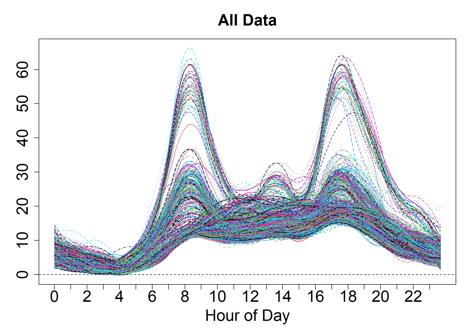
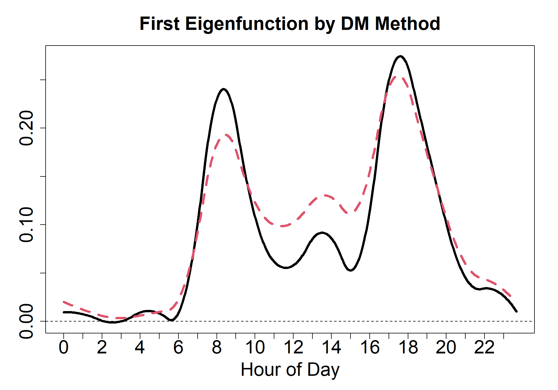
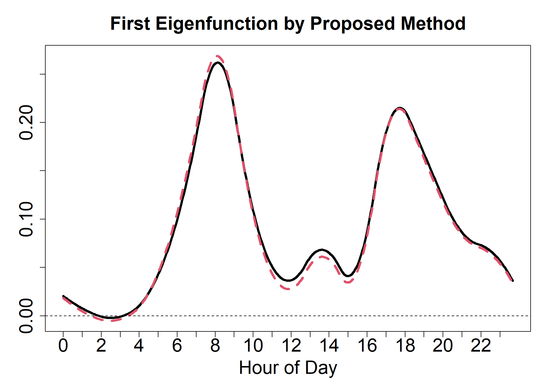
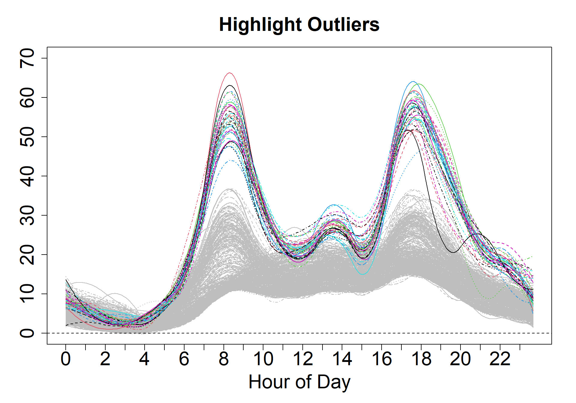
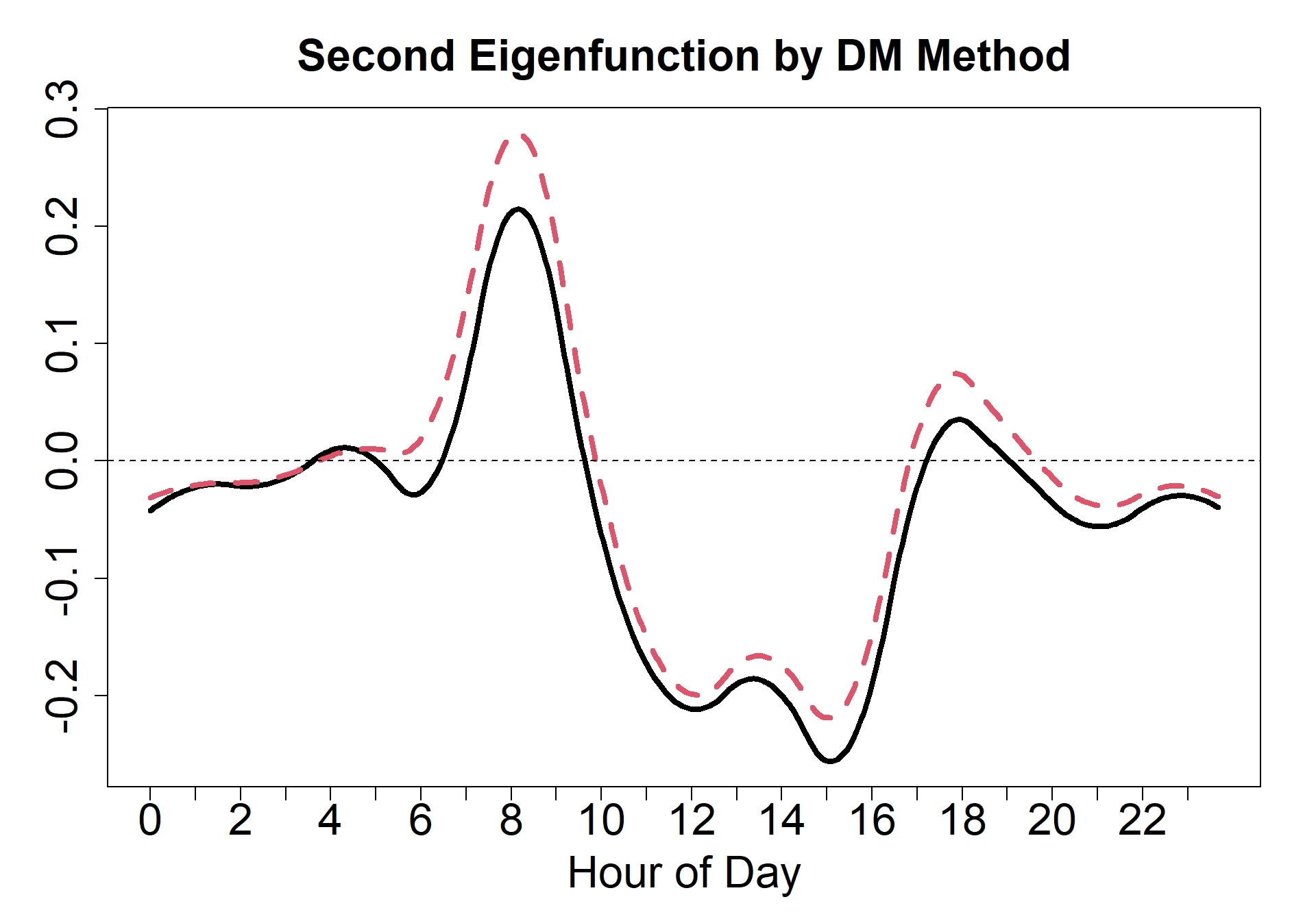
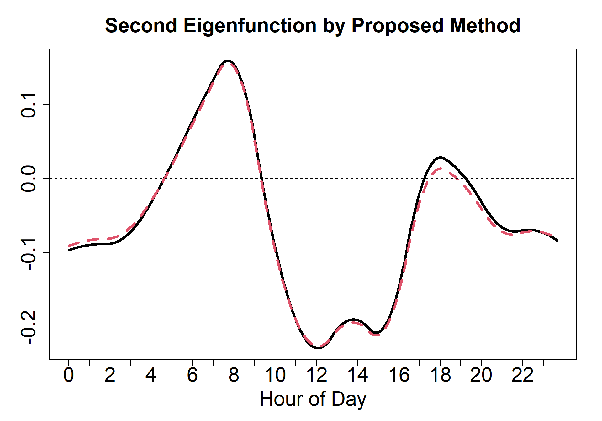
Figure 3: Estimated eigenfunctions of the proposed autocovariance and the autocovariance in Dubey and Müller’s method, abbreviated as DM, with outliers included versus outliers removed. The solid black lines represent the estimated eigenfunctions with data including outliers, and the red dashed lines represent those with data excluding outliers.

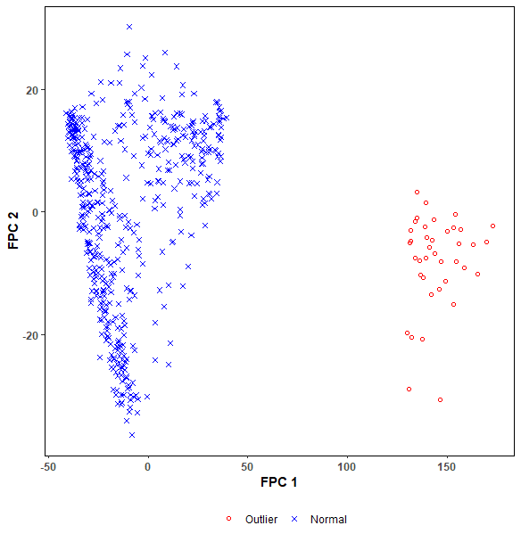
Figure S10: Pairwise plot of the first two FPC scores, distinguished by the normal point and the outliers.

Finally, we investigate the robustness properties of Dubey and Müller’s method and our proposed method by performing analysis with and without outliers. For illustrative purposes, we focus on analyzing a subset of 558 from the 1273 daily Fréchet median distance trajectories, for easier visualization in demonstrating the influence of potential outliers on eigenfunction estimations. Figure 3 displays the first two estimated eigenfunctions by our proposed autocovariance and the autocovariance in Dubey and Müller’s method. To compare the robustness of these two methods, the selection of the subset of daily Fréchet median distance trajectories is based on their Frobenius norm, as the Fréchet median distance trajectories convey the overall daily departure from the center of the space of sample Laplacian matrices. The top left figure in Fig. 3 shows the general shape of the spline smoothed 588 data, and the bottom left figure highlights 39 identified outliers. By comparing eigenfunctions estimated with and without outliers, our method can be seen to be robust, as the eigenfunctions overlap in Fig. 3. However, the estimated eigenfunctions by Dubey and Müller’s method are clearly more sensitive to the presence of outliers. Moreover, we can use the pairwise plots of the first two functional principal scores scores to detect outliers. Figure S10 in the Supplementary Material illustrates the successful identification of outliers using our proposed method through pairwise plots of the first two functional principal component scores.

5 Simulation Study

We illustrate our method by simulations of samples of time-varying networks with 20 nodes. To facilitate comparison, we use a similar network generation technique to that in Dubey and Müller, (2021) with three different community structures. Details of data generation can be found in the supplementary material. We let the community memberships of the nodes stay fixed in time, while the edge connectivity strengths between the communities change with time. We first generate the network adjacency matrices $A_{i}(t)$ by (S10.1) in the supplementary material and the trajectories are represented as graph Laplacians $X_{i}(t)=D_{i}(t)-A_{i}(t)$, where $D_{i}(t)$ is a diagonal matrix whose diagonal elements are equal to the sum of the corresponding row elements in $A_{i}(t)$. We generate 100 samples for each group and we have 300 samples in total. Adopting the Frobenius norm in the space of graph Laplacians, the Fréchet median network at time $t$ is obtained via the extrinsic method whose details are given in the supplementary material, and we obtain the Frobenius distance trajectories of the individual subjects from the Fréchet median trajectory. We then carry out robust functional principal component analysis of the generated distance trajectories.

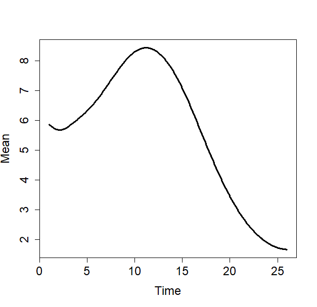
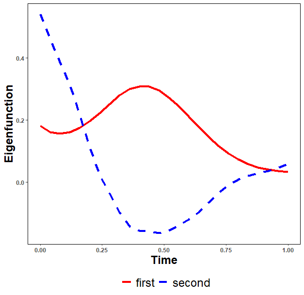
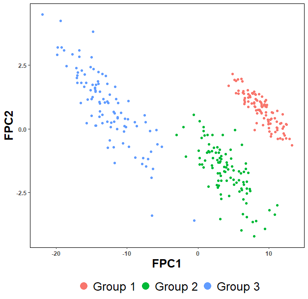
Figure 4: Sample mean function (left plot) and eigenfunctions (middle plot) and the scatter plot of first two functional principal component (right plot) obtained from the robust functional component analysis of the distance trajectories for networks.

The results of robust functional principal component analysis are shown in Fig. 4. The proposed method is seen to perform well in recovering the groups in the scatter plot of the second versus first functional principal component. Groups 1 and 2 are found to have closer cluster centers than Groups 1 and 3. A detailed explanation may be found in the Supplementary Material.

To examine the finite-sample robustness of the proposed method, we also examine situations where a portion of the simulated data are contaminated by outliers. The percentages of outliers considered in our simulation are $\{0.05,0.1,\ldots,0.4\}$. We considered several types of contamination but report only the worst-case scenario. Outliers are generated through adding a shift of 0.5 to the time varying connectivity weights and scaling the weights value by five times. In each settings above, 200 simulation replications were conducted.

Figure 5: Simulated data with outliers generated by extreme values with a shift in time varying connectivity weights. Mean absolute angle (left), empirical bias (middle) and Mean Squared Error (right) of the leading eigenfunction. DM method stands for Dubey and Müller’s method.

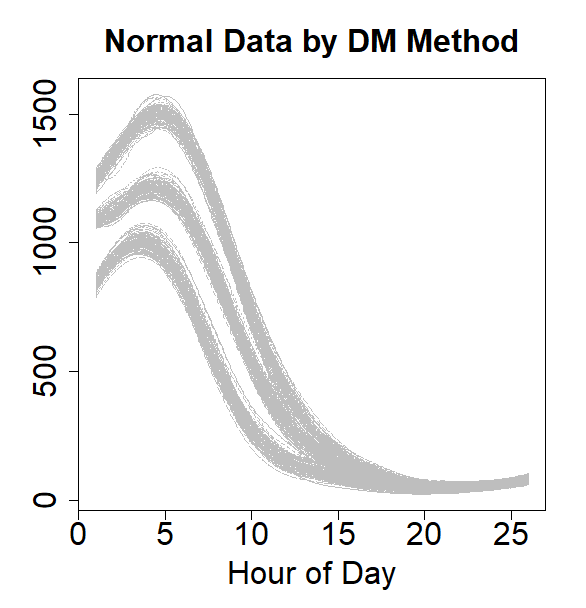
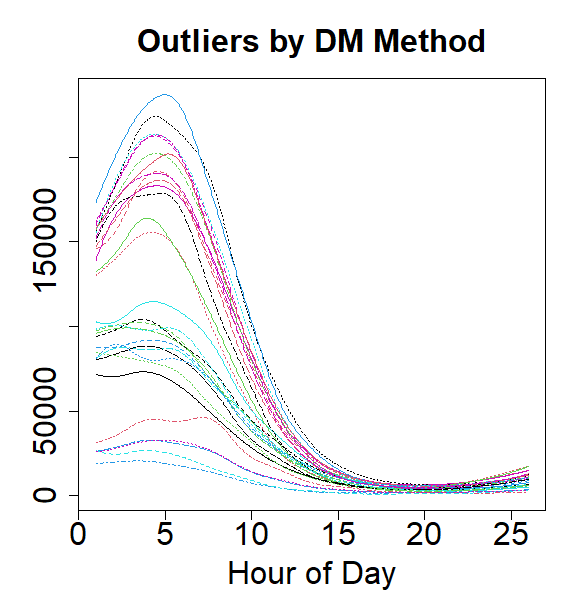
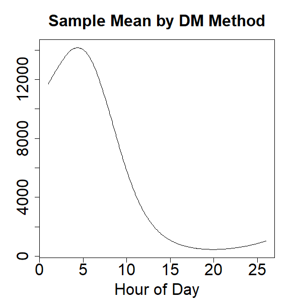
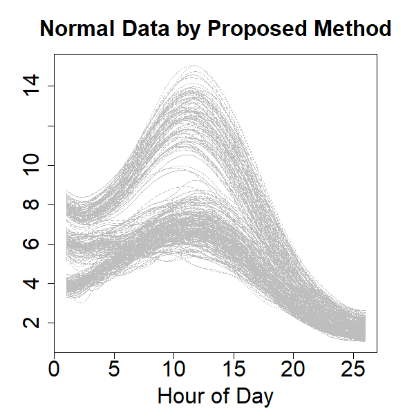
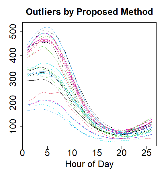
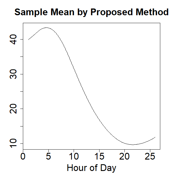
Figure S8: Simulated data with outliers and the percentage of outliers is 0.1. The first row is for the Fréchet variance trajectories produced by Dubey and Müller’s method. The second row is for the Fréchet median distance trajectories produced by our proposed method.

We consider Dubey and Müller’s method proposed by Dubey and Müller, (2021) for comparison. The performance of the eigenfunction estimation is measured by the mean absolute angle, the empirical bias and the mean integrated square error. The mean absolute angle of the $k$-th eigenfunction is given by $\textrm{MEA}=\frac{1}{200}\sum_{t=1}^{200}\arccos(|\langle\hat{\phi}_{k}^{(t)},\bar{\phi}_{k}\rangle|)$ where $\hat{\phi}_{k}^{(t)}$ is the estimate of the $k$-th eigenfunction at the $t$-th replicate and $\bar{\phi}_{k}$ is the Monte Carlo approximation of the unknown population $k$-th eigenfunction under the uncontaminated setting. Figure 5 shows simulation results on the estimation of the leading eigenfunction where our proposed method outperforms Dubey and Müller’s method. Additionally, as the contamination proportion gets closer to the breakdown point 0.4, all of the three measures of the leading eigenfunction increase slower as expected. Our proposed method outperforms Dubey and Müller’s method as their method starts to break down when the contamination ratio equal to 0.05. The reason for the failure of Dubey and Müller’s method can be found in Fig. S8 in the supplementary material. In Dubey and Müller’s method, the Fréchet variance trajectories are the deviations from the Fréchet mean trajectory and they are sensitive to the outliers. Figure S8 in the supplementary material shows that, due to the existence of outliers, the Fréchet mean trajectory shifts to the left side, resulting in a shift of the Fréchet variance trajectories. As there exist a large change in the shapes of Fréchet variance trajectories after the contamination, it is not surprising that the Dubey and Müller’s method will break down with a small number of outliers.

6 Discussion

We provide a framework for the analysis of time-varying random object data in presence of outlying objects, where the random objects can take values in a general metric space, by defining a generalized notion of median function in the object space. The key to our approach is that we develop a novel robust functional principal component analysis autocovariance operator which can be applied to distance functions of the subject-specific curves from the median function. The proposed robust estimator of the autocovariance operator is designed to deal with the nonnegative and dependence properties of the subject-specific curves from the median function.

Our numerical studies on network Laplacian matrix data show that our proposed robust functional principal component analysis can be used to detect clusters and outliers. Additionally, as we demonstrate in simulation studies and real data analysis, our proposed method outperforms the existing methodology for time-varying random object data (Dubey and Müller, 2021) with respect to robustness, but typically gives comparable performance when outlying objects are not present in the sample.

Supplementary material

The Supplementary Material consists of overview of the theoretical derivations, technical lemmas and propositions, proofs of theorems, additional figures for numerical studies, data generation and calculation methods for network Laplacians.

Appendix

This Appendix introduces six useful assumptions. These assumptions are discussed below.

Assumption 1.

For each $t\in[0,1]$, the pointwise Fréchet median $\mu_{\rm GM}(t)$ given in (2.1) exists and is unique, and

$$\inf_{t\in[0,1]}\inf_{\omega\in\Omega:d(\omega,\mu_{\rm GM}(t))>\gamma}E[d(\omega,X(t))]-E[d(\mu_{\rm GM}(t),X(t))]>0$$

for any $\gamma>0$. Additionally, there exists a $\tau=\tau(\gamma)>0$ such that

$$\lim_{n\to\infty}P\left(\inf_{t\in[0,1]}\inf_{\omega\in\Omega:d(\omega,\hat{\mu}_{\rm GM}(t))>\gamma}\frac{1}{n}\sum_{i=1}^{n}\{d(\omega,X_{i}(t))-d(\hat{\mu}_{\rm GM}(t),X_{i}(t))\}>\tau\right)=1.$$

Assumption 2.

There exists $\rho>0$, $D>0$ and $\beta>1$ such that

$$\inf_{t\in[0,1]}\inf_{\omega\in\Omega:d(\omega,\mu_{\rm GM}(t))<\rho}\left\{E[d(X(t),\omega)]-E[d(X(t),\mu_{\rm GM}(t))]-Dd^{\beta}(\omega,\mu_{\rm GM}(t))\right\}\geq 0,$$

Assumption 3.

For some $0<\alpha\leq 1$, the random function $X(\cdot)$ is defined on $[0,1]$ and takes values in $\Omega$ and suppose to be $\alpha$-Hölder continuous. Denote the space of all such functions as $\Omega^{[0,1]}$. That is, for nonnegative $G:\Omega^{[0,1]}\to\mathbb{R}^{+}$ with $E[G(X(\cdot))^{2}]<\infty$, it holds almost surely,

$$d(X(s),X(t))\leq G(X(\cdot))|s-t|^{\alpha}.$$

Assumption 4.

For $I(\delta)=\int_{0}^{1}\sup_{t\in[0,1]}\sqrt{\log N(\varepsilon\delta,B_{\delta}(\mu_{\rm GM}(t)),d)}d\varepsilon$, it holds that $I(\delta)=O(1)$ as $\delta\to 0$, where $B_{\delta}(\mu_{\rm GM}(t))=\{\omega\in\Omega:d(\omega,\mu_{\rm GM}(t))<\delta\}$ is the $\delta$-ball around $\mu_{\rm GM}(t)$ and $N(\gamma,B_{\delta}(\mu_{\rm GM}(t)),d)$ is the covering number.

Assumption 5.

For each $j\geq 1$, the eigenvalue $\lambda_{j}(C)$ has multiplicity one, i.e., it holds that $\delta_{j}>0$ where $\delta_{j}=\min_{1\leq l\leq j}(\lambda_{l}-\lambda_{l+1})$.

Assumption 6.

$V(\cdot)$ is weakly functional coordinate symmetric. That is, for any positive integers $d\leq d^{\prime}\leq\infty$ with $d<\infty$ and any orthonormal bases $\{\psi_{1}(\cdot),\ldots,\psi_{d}(\cdot)\}$ in $\mathcal{H}$, $(\langle V(\cdot)-\widetilde{V}(\cdot),\psi_{1}(\cdot)\rangle,\ldots,\langle V(\cdot)-\widetilde{V}(\cdot),\psi_{d}(\cdot)\rangle)^{\top}=\Psi Z_{\psi}$ in distribution, where $\Psi$ is a $d\times d^{\prime}$ matrix only depending on $\{\psi_{1}(\cdot),\ldots,\psi_{d}(\cdot)\}$ such that $\Psi\Psi^{\top}=I_{d}$, the $d$-dimensional identity matrix, and $Z_{\psi}\in\mathbb{R}^{d^{\prime}}$ is coordinatewise symmetric in the sense that $GZ_{\psi}=Z_{\psi}$ in distribution for any diagonal matrix $G$ with diagonal elements $G_{jj}\in\{-1,1\}$.

Assumption 1 guarantees uniform convergence of the sample Fréchet median trajectory to its population target as it implies $\sup_{t\in[0,1]}d(\hat{\mu}_{\rm GM}(t),\mu_{\rm GM}(t))=o_{P}(1)$. The latter result is the third statement in Proposition 1. Measurability issues of the sample Fréchet median function can be dealt with by considering outer probability measures, as with $M$-estimators; see van der Vaart and Wellner, (1996). Assumption 2 is standard for M-estimators and characterize the local curvature of the target function to be minimized near the minimum. The curvature is characterized by $\beta$, which features in the resulting rate of convergence. Assumption 3 is a mild smoothness assumption satisfied for certain value of $\alpha$ by many common Euclidean-valued random processes. Assumption 4 is a bound on the covering number, defined e.g. in van der Vaart and Wellner, (1996), of the object metric space and is satisfied by several commonly encountered random objects. Assumption 5 is needed to show the asymptotic property of the estimated eigenfunctions. It is worth noting that Assumptions 1-5 are the same conditions used in Dubey and Müller, (2020, 2021) and object spaces that satisfy these assumptions include graph Laplacians of networks with the Frobenius metric, univariate probability distributions with the 2-Wasserstein metric and correlation matrices of a fixed dimension with the Frobenius metric (Petersen and Müller, 2019). Additionally, these metric spaces satisfy Assumption 2 with $\beta=2$ (Dubey and Müller, 2021). Assumption 6 is the weakest condition to our knowledge in the literature to ensure that the robust estimator of the autocovariance operator has the same set of eigenfunctions as those of the regular covariance function. This condition is proposed by Wang et al., (2023), which generalize the functional coordinate symmetry condition used in Gervini, (2008). Wang et al., (2023) shows that the weak functional coordinate symmetry condition, Assumption 6, permits arbitrary marginal distributions.

SUPPLEMENTARY MATERIAL
for
Robust Functional Principal Component Analysis for Non-Euclidean Random Objects
by
Jiazhen Xu,    Andrew T. A. Wood    and Tao Zou

This supplementary material consists of five parts. §S7 overviews the theoretical derivations. §S8 introduces the technical lemmas and propositions. §S9 contains the proof of the theorems and corollaries. §S10 covers the definition of network Laplacians,the data generation of network Laplacians and the corresponding extrinsic calculation method for Fréchet medians. §S11 presents additional figures for numerical studies.

S7 Overview of the Theoretical Derivations

For any generic functional $h(t),t\in[0,1]$, denote $\check{h}=h(\cdot)$ be an element located in the Hilbert space $\mathcal{H}$. Denote $\|\cdot\|$ be the Hilbert norm, $\|\cdot\|_{2}$ be the $L_{2}$-norm. For any generic function classes $\mathcal{F}$ and $\mathcal{G}$, denote all pairwise sums as $\mathcal{F}+\mathcal{G}=\{\check{f}+\check{g}:\check{f}\in\mathcal{F},\check{g}\in\mathcal{G}\}$ and denote all pairwise products as $\mathcal{F}\cdot\mathcal{G}=\{\check{f}\check{g}:\check{f}\in\mathcal{F},\check{g}\in\mathcal{G}\}$. For a generic object space $(\Omega,d)$, denote $d(\check{\omega}_{1},\check{\omega}_{2})$ be the trajectory of $d(\omega_{1}(t),\omega_{2}(t))$ for $\omega_{1}(t),\omega_{2}(t)\in\Omega$ and $t\in[0,1]$, that is $d(\check{\omega}_{1},\check{\omega}_{2})\in\mathcal{H}$ and $d(\check{\omega}_{1},\check{\omega}_{2})(t)=d(\omega_{1}(t),\omega_{2}(t))$. For two generic measurable spaces $(\Omega_{1},P_{1})$ and $(\Omega_{2},P_{2})$, denote $P_{1}\otimes P_{2}$ be the product measure on the product measurable space $\Omega_{1}\times\Omega_{2}$.

In order to derive Theorem 1, we first observe that

$$\sqrt{n}\left(\hat{C}_{\rm WPU}(s,t)-C_{\rm WPU}(s,t)-U_{\hat{\mu}_{GM}}(s,t)\right)$$

$$= \sqrt{n}\left(\hat{C}_{\rm WPU}(s,t)-\widetilde{C}_{\rm WPU}(s,t)-U_{\hat{\mu}_{GM}}(s,t)\right)+\sqrt{n}\left(\widetilde{C}_{\rm WPU}(s,t)-C_{\rm WPU}(s,t)\right).$$

We can show that the first term converges to zero in probability while the second term converge weakly to a Gaussian process.

A critical step in establishing uniform convergence of the plug-in estimator in the symmetrized spatial sign autocovariance surface $\widetilde{C}_{\rm WPU}$ given by $\hat{C}_{\rm WPU}$ is to find an upper bound for the quantity

$$E(\sup_{s,t\in[0,1],\check{\omega}:d_{\infty}(\check{\omega},\mu_{\rm GM})<\delta}|U_{n}(\check{\omega},s,t)-U(\check{\omega},s,t)|)$$

for $\delta>0$, where $d_{\infty}(\check{\omega},\mu_{\rm GM})=\sup_{t\in[0,1]}d(w(t),\mu_{\rm GM}(t))$. Here, for a function $\check{\omega}$ with $\omega(l)$ taking values in $\Omega$ for all $l\in[0,1]$ and $s,t\in[0,1]$, define

$$U_{n}(\check{\omega},s,t)=\frac{1}{n(n-1)}\sum_{i=1}^{n}\sum_{j\neq i}f_{\check{\omega},s,t}(X_{i}(\cdot),X_{j}(\cdot))~{}{\rm and}~{}U(\check{\omega},s,t)=E[f_{\check{\omega},s,t}(X(\cdot),\widetilde{X}(\cdot))],$$

where

$$f_{\check{\omega},s,t}(\check{x},\check{y})= \left[d(\omega(s),x(s))-d(\omega(s),y(s))\right]\left[d(\omega(t),x(t))-d(\omega(t),y(t))\right]$$

$$\times\xi^{2}\left(\|d(\check{\omega},\check{x})-d(\check{\omega},\check{y})\|\right)$$

$$-\left[d(\mu_{\rm GM}(s),x(s))-d(\mu_{\rm GM}(s),y(s))\right]\left[d(\mu_{\rm GM}(t),x(t))-d(\mu_{\rm GM}(t),y(t))\right]$$

$$\times\xi^{2}\left(\|d(\mu_{\rm GM},\check{x})-d(\mu_{\rm GM},\check{y})\|\right).$$

For this, we can consider a function class

$$\mathcal{F}_{\delta}^{\rm total}=\{f_{\check{\omega},s,t}:s,t\in[0,1],d_{\infty}(\check{\omega},\mu_{\rm GM})<\delta\}$$

and apply empirical process theory to show the uniform convergence of $\hat{C}_{\rm WPU}$. An envelope function for this class is the constant function $F^{\rm total}(\check{x},\check{y})=(4+1/Q)M\delta$, where $M$ is the diameter of $\Omega$. The $L_{2}$ norm of the envelope function is $\|F^{\rm total}\|_{2}=(4+1/Q)M\delta$. By Theorem 2.14.2 of van der Vaart and Wellner, (1996),

$$E\left(\sup_{s,t\in[0,1],\check{\omega}:d_{\infty}(\check{\omega},\mu_{\rm GM})<\delta}|U_{n}(\check{\omega},s,t)-U(\check{\omega},s,t)|\right)$$ (S7.1)

$$\leq \frac{\left(4+\frac{1}{Q}\right)M\delta J_{[]}(1,\mathcal{F}_{\delta}^{\rm total},L_{2}(P\otimes P))}{\sqrt{n}},$$ (S7.2)

where $J_{[]}(1,\mathcal{F}_{\delta}^{\rm total},L_{2}(P\otimes P))$ is the bracketing integral of the function class $\mathcal{F}_{\delta}^{\rm total}$, which is

$$J_{[]}(1,\mathcal{F}_{\delta}^{\rm total},L_{2}(P\otimes P))=\int_{0}^{1}\sqrt{1+\log N_{[]}(\varepsilon\|F^{\rm total}\|_{2},\mathcal{F}_{\delta}^{\rm total},L_{2}(P\otimes P))}d\varepsilon.$$ (S7.3)

We can show that, under Assumptions 1-4,

$$J_{[]}(1,\mathcal{F}_{\delta}^{\rm total},L_{2}(P\otimes P))=O\left(\sqrt{\log\frac{1}{\delta}}\right)~{}{\rm as}~{}\delta\to 0.$$

To derive the above result, we consider some generating function classes and use preservation of Donsker classes. The function classes we consider are

$$\mathcal{F}^{(1)}=\{f^{(1)}(x,y;t),t\in[0,1]\}~{}{\rm with}~{}f^{(1)}(x,y;t)=d(x(t),\mu_{\rm GM}(t))-d(y(t),\mu_{\rm GM}(t)),$$

$$\mathcal{F}^{(2)}=\{f^{(2)}(x,y;\omega,t),t\in[0,1]\}~{}{\rm with}~{}f^{(2)}(x,y;\omega,t)=d(x(t),\omega)-d(y(t),\omega),$$

and $\mathcal{F}_{\delta}^{(3)}=\{f^{(3)}(x,y;\omega,t),t\in[0,1],d(\omega,\mu_{\rm GM}(t))<\delta\}$ with

$$f^{(3)}(x,y;\omega,t)=d(\omega,x(t))-d(\omega,y(t))-d(\mu_{\rm GM}(t),x(t))+d(\mu_{\rm GM}(t),y(t)).$$

See Proposition 5 for details.

S8 Auxiliary Lemmas

Proposition 1.

If the random object process $\{X(t)\}_{t\in[0,1]}$ has almost surely continuous sample functions, then under Assumption 1, for $t\in[0,1]$ and a sequence $\{t_{n}\}\in[0,1]$ such that $t_{n}\to t$,

$$d(\mu_{\rm GM}(t_{n}),\mu_{\rm GM}(t))\to 0.$$ (S8.1)

For the empirical Fréchet median defined in (2.1), we also have

$$d(\hat{\mu}_{\rm GM}(t),\mu_{\rm GM}(t))=o_{p}(1),$$ (S8.2)

for all $t\in[0,1]$. Furthermore, under Assumption 1,

$$\sup_{t\in[0,1]}d(\hat{\mu}_{\rm GM}(t),\mu_{\rm GM}(t))=o_{p}(1).$$ (S8.3)

Proof.

This proof consists of three steps, which are corresponding to the three statement (S8.1), (S8.2) and (S8.3), respectively. The first statement (S8.1) shows that the population Fréchet median $\mu_{\rm GM}$ is continuous. The second statement shows the pointwise convergence of $\mu_{\rm GM}$ for any $t\in[0,1]$ to zero. The third statement (S8.3) shows the uniform convergence of $\hat{\mu}_{\rm GM}$.

Proof of Part I. Note that almost surely continuous sample functions on the compact interval $[0,1]$ are uniformly continuous. Additionally, $\Omega$ is totally bounded and thus has finite diameter. By the bounded convergence theorem, for all $t\in[0,1]$ and sequences ${t_{n}}\in[0,1]$ such that $t_{n}\to t$, there exists a $\delta>0$ for every $\varepsilon>0$ such that whenever $|t_{n}-t|<\delta$, one has $E[d(X(t_{n}),X(t))]<\varepsilon$ for all but finitely many $n$.

For the process $E[d(\omega,X(t))]$, using the linearity and monotonicity of the Lebesgue integral, we have

$$\left|E[d(\omega,X(t_{n}))]-E[d(\omega,X(t))]\right| =\left|E[d(\omega,X(t_{n}))-d(\omega,X(t))]\right|$$

$$\leq E\left[\left|d(\omega,X(t_{n}))-d(\omega,X(t))\right|\right]$$

$$\leq E[d(X(t_{n}),X(t))],$$

where the last inequality holds by using the triangle inequality. Therefore, for any $\widetilde{\varepsilon}>0$, there exists a $\widetilde{\delta}>0$ such that whenever $|t_{n}-t|<\widetilde{\delta}$, it holds that

$$\sup_{\omega\in\Omega}|E[d(\omega,X(t_{n}))]-E[d(\omega,X(t))]|<\widetilde{\varepsilon}.$$ (S8.4)

Note that by the definition of the population Fréchet median given in (2.1), we always have $d(\mu_{\rm GM}(t),X(t))=\min_{\omega\in\Omega}d(\omega,X(t))$ for $t\in[0,1]$. This result, together with (S8.4), gives

$$\left|E[d(\mu_{\rm GM}(t_{n}),X(t))]-E[d(\mu_{\rm GM}(t),X(t))]\right|$$

$$= \left|E[d(\mu_{\rm GM}(t_{n}),X(t))]-E[d(\mu_{\rm GM}(t_{n}),X(t_{n}))]+E[d(\mu_{\rm GM}(t_{n}),X(t_{n}))]-E[d(\mu_{\rm GM}(t),X(t))]\right|$$

$$\leq \left|E[d(\mu_{\rm GM}(t_{n}),X(t))]-E[d(\mu_{\rm GM}(t_{n}),X(t_{n}))]\right|+\left|E[d(\mu_{\rm GM}(t_{n}),X(t_{n}))]-E[d(\mu_{\rm GM}(t),X(t))]\right|$$

$$\leq \sup_{\omega\in\Omega}\left|E[d(\omega,X(t_{n}))]-E[d(\omega,X(t))]\right|+\left|\min_{\omega\in\Omega}E[d(\omega,X(t_{n}))]-\min_{\omega\in\Omega}E[d(\omega,X(t))]\right|$$

$$\leq 2\sup_{\omega\in\Omega}\left|E[d(\omega,X(t_{n}))]-E[d(\omega,X(t))]\right|<2\widetilde{\varepsilon}.$$ (S8.5)

Now we assume that $d(\mu_{\rm GM}(t_{n}),\mu_{\rm GM}(t))$ does not converge to zero. Then for any $\bar{\delta}>0$, there exist a $\gamma>0$ and a subsequence $\{t_{n_{k}}\}$ of $\{t_{n}\}$ such that $|t_{n_{k}}-t|<\bar{\delta}$ and $d(\mu_{\rm GM}(t_{n_{k}}),\mu_{\rm GM}(t))>\gamma$. By Assumption 1, we then obtain

$$\left|E[d(\mu_{\rm GM}(t_{n_{k}}),X(t))]-E[d(\mu_{\rm GM}(t),X(t))]\right|$$

$$\geq \left|\inf_{\omega\in\Omega:d(\omega,\mu_{\rm GM}(t))>\gamma}E[d(\omega,X(t))]-E[d(\mu_{\rm GM}(t),X(t))]\right|>0.$$

This leads to a contradiction for (S8) when setting $\widetilde{\varepsilon}=\Big{|}\inf_{\omega\in\Omega:d(\omega,\mu_{\rm GM}(t))>\gamma}E[d(\omega,X(t))]$ $-E[d(\mu_{\rm GM}(t),X(t))]\Big{|}/2$. This completes the proof of the first statement in Proposition 1.

Proof of Part II. The proof is quite similar to the one of Theorem 1 in Petersen and Müller, (2019) and thus is omitted.

Proof of Part III. By Theorem 1.5.4 in van der Vaart and Wellner, 1996, we only need to show the pointwise convergence of $Z_{n}(t)=d(\hat{\mu}_{\rm GM}(t),\mu_{\rm GM}(t))$ to zero and the uniform asymptotic equicontinuity of $Z_{n}(t)$. Note that by the second statement in Proposition 1, we have for any $t\in[0,1]$, $d(\hat{\mu}_{\rm GM}(t),\mu_{\rm GM}(t))=o_{p}(1)$. Therefore, it is suffices to show that, for any $\eta>0$,

$$\lim_{\delta\to 0}\limsup_{n\to\infty}P\left(\sup_{|s-t|<\delta}|Z_{n}(s)-Z_{n}(t)|>\eta\right)=0.$$

Note that by the triangle inequality, $|Z_{n}(s)-Z_{n}(t)|\leq d(\mu_{\rm GM}(s),\mu_{\rm GM}(t))+d(\hat{\mu}_{\rm GM}(s),\hat{\mu}_{\rm GM}(t))$. This result, together with the first statement in Proposition 1, implies that we only need to show that, for any $\widetilde{\eta}>0$,

$$\lim_{\delta\to 0}\limsup_{n\to\infty}P\left(\sup_{|s-t|<\delta}d(\hat{\mu}_{\rm GM}(s),\hat{\mu}_{\rm GM}(t))>\widetilde{\eta}\right)=0.$$ (S8.6)

To establish (S8.6), we first define the events

$$A_{n}=\left\{\sup_{|s-t|<\delta}\left|\frac{1}{n}\sum_{i=1}^{n}[d(\hat{\mu}_{\rm GM}(s),X_{i}(t))-d(\hat{\mu}_{\rm GM}(t),X_{i}(t))]\right|\geq\tau(\widetilde{\eta})\right\},$$

and $B=\left\{\sup_{|s-t|<\delta}d(\hat{\mu}_{\rm GM}(s),\hat{\mu}_{\rm GM}(t))>\widetilde{\eta}\right\}$ with $\tau(\widetilde{\eta})$ defined in Assumption 1.

By using similar techniques to those used in (S8), we have

$$\left|\frac{1}{n}\sum_{i=1}^{n}[d(\hat{\mu}_{\rm GM}(s),X_{i}(t))-d(\hat{\mu}_{\rm GM}(t),X_{i}(t))]\right|\leq 2\sup_{\omega\in\Omega}\left|\frac{1}{n}\sum_{i=1}^{n}[d(\omega,X_{i}(s))-d(\omega,X_{i}(t))]\right|.$$ (S8.7)

On the other hand, note that $\sup_{|s-t|<\delta}d(X(s),X(t))\to 0$ as $\delta\to 0$ almost surely as the functions $X(\cdot)$ are continuous and the domain $[0,1]$ is compact. By the bounded convergence theorem, we have

$$\lim_{\delta\to 0}E\left[\sup_{|s-t|<\delta}d(X(s),X(t))\right]=0.$$

This result, in conjunction with Markov’s inequality and the triangle inequality, implies that, for any $\theta>0$,

$$P\left(\sup_{|s-t|<\delta}\sup_{\omega\in\Omega}\left|\frac{1}{n}\sum_{i=1}^{n}[d(\omega,X_{i}(s))-d(\omega,X_{i}(t))]\right|>\theta\right)$$

$$\leq \frac{ME\left(\sup_{|s-t|<\delta}\frac{1}{n}\sum_{i=1}^{n}d(X_{i}(s),X_{i}(t))\right)}{\theta}$$

$$= \frac{ME\left(\sup_{|s-t|<\delta}d(X(s),X(t))\right)}{\theta}\to 0,$$ (S8.8)

as $\delta\to 0$ and $M={\rm diam}(\Omega)$.

Given (S8.7) and the definition of the events $A_{n}$ and $B$, it can be readily seen that

$$P\left(\sup_{|s-t|<\delta}d(\hat{\mu}_{\rm GM}(s),\hat{\mu}_{\rm GM}(t))>\widetilde{\eta}\right)$$

$$= P(A_{n}\cap B)+P(A_{n}^{C}\cap B)$$

$$\leq P\left(\sup_{|s-t|<\delta}2\sup_{\omega\in\Omega}\left|\frac{1}{n}\sum_{i=1}^{n}[d(\omega,X_{i}(s))-d(\omega,X_{i}(t))]\right|\geq\tau(\widetilde{\eta})\right)+P(A_{n}^{C}\cap B).$$ (S8.9)

Note that by choosing $\theta=\tau(\widetilde{\eta})/2$ in (S8), we have

$$\lim_{\delta\to 0}P\left(\sup_{|s-t|<\delta}2\sup_{\omega\in\Omega}\left|\frac{1}{n}\sum_{i=1}^{n}[d(\omega,X_{i}(s))-d(\omega,X_{i}(t))]\right|\geq\tau(\widetilde{\eta})\right)=0.$$

By Assumption 1, $\lim_{n\to\infty}P(A_{n}^{C}\cap B)=0$. Therefore, we can conclude that (S8.6) holds, which completes the proof of the third statement in Proposition 1. ∎

Proposition 2.

Under Assumptions 1-4, it holds for the function class $\mathcal{G}_{\delta}=\{g_{\omega,t}:t\in[0,1],$ $d(\omega,\mu_{\rm GM}(t))<\delta\}$ that $J_{[]}(1,\mathcal{G}_{\delta},L^{2}(P))=O(\sqrt{\log 1/\delta})$ as $\delta\to 0$, where $g_{\omega,t}(x)=d(\omega,x(t))-d(x(t),\mu_{\rm GM}(t))$.

Proof.

Note that by triangle inequality,

$$|g_{\omega,t}(x)-g_{\widetilde{\omega},\widetilde{t}}(x)| \leq|g_{\omega,t}(x)-g_{\widetilde{\omega},t}(x)|+|g_{\widetilde{\omega},t}(x)-g_{\widetilde{\omega},\widetilde{t}}(x)|$$

$$\leq d(\omega,\widetilde{\omega})+2d(x(t),x(\widetilde{t}))+d(\mu_{\rm GM}(t),\mu_{\rm GM}(\widetilde{t})).$$ (S8.10)

Since $X(\cdot)$ has almost surely continuous, the first statement in Proposition 1 implies that $\mu_{\rm GM}$ is uniformly continuous. Thus we can always find $\widetilde{t}$ close to $t$ such that $d(\mu_{\rm GM}(t),\mu_{\rm GM}(\widetilde{t}))<\rho$. By Assumptions 2 and 3,

$$d^{\beta}(\mu_{\rm GM}(t),\mu_{\rm GM}(\widetilde{t}))$$

$$\leq \frac{1}{2}D^{-1}\left(E[d(X(t),\mu_{\rm GM}(\widetilde{t}))]-E[d(X(t),\mu_{\rm GM}(t))]+E[d(X(\widetilde{t}),\mu_{\rm GM}(t))]-E[d(X(\widetilde{t}),\mu_{\rm GM}(\widetilde{t}))]\right)$$

$$\leq D^{-1}E[d(X(t),X(\widetilde{t}))]$$

$$\leq D^{-1}E[G(X(\cdot))]|t-\widetilde{t}|^{\alpha}.$$

Let $K=[D^{-1}E(G(X(\cdot)))]^{1/\beta}$, for all $|t-\widetilde{t}|<\left(\frac{\rho}{K}\right)^{\beta/\alpha}$,

$$d(\mu_{\rm GM}(t),\mu_{\rm GM}(\widetilde{t}))\leq K|t-\widetilde{t}|^{\frac{\alpha}{\beta}}.$$

This result, together with (S8) and Assumption 3, implies that for some $U$ such that $E[U^{2}]<\infty$,

$$|g_{\omega,t}(x)-g_{\widetilde{\omega},\widetilde{t}}(x)|\leq U\left(d(\omega,\widetilde{\omega})+d(x(t),x(\widetilde{t}))+d(\mu_{\rm GM}(t),\mu_{\rm GM}(\widetilde{t}))\right),$$

and thus for some constant $L>0$,

$$\|g_{\omega,t}-g_{\widetilde{\omega},\widetilde{t}}\|_{L^{2}}\leq L\left(d(\omega,\widetilde{\omega})+|t-\widetilde{t}|^{\alpha}+d(\mu_{\rm GM}(t),\mu_{\rm GM}(\widetilde{t}))\right).$$

Since we aim to study the asymptotic behavior as $\delta\to 0$, without loss of generality, we can let $\delta<\min\{\rho,1\}$. Then for any given $0<u<1$, if we choose $\widetilde{t}$ to be such that $|t-\widetilde{t}|<\left(\frac{\delta u}{K}\right)^{\beta/\alpha}$, then $d(\mu_{\rm GM}(t),\mu_{\rm GM}(\widetilde{t}))$ is less than or equal to $\delta u$, which means $\mu_{\rm GM}(\widetilde{t})$ is contained in $B_{\delta}(\mu_{\rm GM}(t))$, and therefore within $B_{2\delta}(\mu_{\rm GM}(t))$. Let $t_{1},\ldots,t_{K}$ be a $\left(\frac{\delta u}{K}\right)^{\beta/\alpha}$-net for $[0,1]$ with the metric $|\cdot|$ and $\omega_{1}^{t_{j}},\ldots,\omega_{L}^{t_{j}}$ be a $u$-net for $B_{2\delta}(\mu_{\rm GM}(t_{j}))$ with metric $d$. Then for any $t\in[0,1]$ and $\omega$ such that $d(\omega,\mu_{\rm GM}(t))<\delta$, one can find $t_{j}$ and $\omega_{k}^{t_{j}}$ such that for some constant $L^{\prime}>0$,

$$\|g_{\omega,t}-g_{\omega_{k}^{t_{j}},t_{j}}\|_{L^{2}}\leq L^{\prime}u.$$

This implies that

$$N_{[]}(L^{\prime}u,\mathcal{G}_{\delta},L^{2}(P))\leq N\left(\left(\frac{\delta u}{K}\right)^{\frac{\beta}{\alpha}},[0,1],|\cdot|\right)\sup_{t\in[0,1]}N(u,B_{2\delta}(\mu_{\rm GM}(t)),d).$$

Thus, we obtain

$$\log N_{[]}(M\delta\varepsilon,\mathcal{G}_{\delta},L^{2}(P))$$

$$\leq \log N\left(\left(\frac{M\delta^{2}\varepsilon}{KL^{\prime}}\right)^{\frac{\beta}{\alpha}},[0,1],|\cdot|\right)+\sup_{t\in[0,1]}\log N\left(\frac{M\delta\varepsilon}{L^{\prime}},B_{2\delta}(\mu_{\rm GM}(t)),d\right)$$

$$\leq \log\left(\widetilde{C}(\varepsilon\delta^{2})^{-\frac{\beta}{\alpha}}\right)+\sup_{t\in[0,1]}\log N\left(\frac{M\delta\varepsilon}{L^{\prime}},B_{2\delta}(\mu_{\rm GM}(t)),d\right),$$

for some constant $\widetilde{C}$. Additionally, note that the envelope function of $\mathcal{G}_{\delta}$ is a constant given by $G(x)=\delta$. Finally, the entropy integral can be bounded as

$$\int_{0}^{1}\sqrt{1+\log N_{[]}(\varepsilon\|G\|_{2},\mathcal{G}_{\delta},L^{2}(P))}d\varepsilon$$

$$= \int_{0}^{1}\sqrt{1+\log N_{[]}(\delta\varepsilon,\mathcal{F}_{\delta},L^{2}(P))}d\varepsilon$$

$$\leq 1+\sqrt{\log(\widetilde{C})}+\int_{0}^{1}\sqrt{-\frac{\beta}{\alpha}\log(\varepsilon\delta^{2})}d\varepsilon+\int_{0}^{1}\sup_{t\in[0,1]}\sqrt{\log N\left(\delta\varepsilon,B_{2\delta}(\mu_{\rm GM}(t)),d\right)}d\varepsilon$$

$$\leq 1+\sqrt{\log(\widetilde{C})}+\sqrt{\frac{\beta}{\alpha}}\left\{\int_{0}^{1}\sqrt{-\log(\varepsilon)}d\varepsilon+\sqrt{-2\log(\delta)}\right\}+\int_{0}^{1}\sup_{t\in[0,1]}\sqrt{\log N\left(\delta\varepsilon,B_{2\delta}(\mu_{\rm GM}(t)),d\right)}d\varepsilon.$$

The above result, in conjunction with Assumption 4, completes the proof. ∎

Proposition 3.

Under Assumptions 1-4,

$$\sup_{t\in[0,1]}\sqrt{n}\left|\frac{1}{n}\sum_{i=1}^{n}\{\hat{V}_{i}(t)-V_{i}(t)\}\right|=o_{p}(1).$$

Proof.

Let $\varepsilon>0$ and $\delta>0$. Note that

$$P\left(\sup_{t\in[0,1]}\sqrt{n}\left|\frac{1}{n}\sum_{i=1}^{n}[d(X_{i}(t),\hat{\mu}_{\rm GM}(t))-d(X_{i}(t),\mu_{\rm GM}(t))]\right|>\varepsilon\right)$$

$$\leq P\left(\inf_{t\in[0,1]}\left(\frac{1}{n}\sum_{i=1}^{n}[d(X_{i}(t),\hat{\mu}_{\rm GM}(t))-d(X_{i}(t),\mu_{\rm GM}(t))]\right)<-\frac{\varepsilon}{\sqrt{n}}\right)$$

$$\leq P\left(\inf_{t\in[0,1],\omega\in\Omega:d(\omega,\mu_{\rm GM}(t))<\delta}\left(\frac{1}{n}\sum_{i=1}^{n}[d(\omega,X_{i}(t))-d(X_{i}(t),\mu_{\rm GM}(t))]\right)<-\frac{\varepsilon}{\sqrt{n}}\right)$$

$$+P\left(\sup_{t\in[0,1]}d(\hat{\mu}_{\rm GM}(t),\mu_{\rm GM}(t))>\delta\right),$$ (S8.11)

where the last inequality holds after employing similar techniques to those used in (S8). Note that the second term in (S8), $P\left(\sup_{t\in[0,1]}d(\hat{\mu}_{\rm GM}(t),\mu_{\rm GM}(t))\right)$, goes to zero due to the third statement in Proposition 1.

For the first term in (S8), we define

$$W_{n}(\omega,t)=\frac{1}{n}\sum_{i=1}^{n}g_{\omega,t}(X_{i})~{}{\rm and}~{}W(\omega,t)=E[g_{\omega,t}(X)],$$

where $g_{\omega,t}(x)=d(\omega,x(t))-d(\mu_{\rm GM}(t),x(t))$ with $\omega\in\Omega$ and $t\in[0,1]$. Based on this construction, we get

$$\sup_{t\in[0,1],\omega\in\Omega:d(\omega,\mu(t))<\delta}|W_{n}(\omega,t)-W(\omega,t)| \geq\left|\sup_{t\in[0,1],\omega\in\Omega:d(\omega,\mu_{\rm GM}(t))<\delta}\left(W_{n}(\omega,t)-W(\omega,t)\right)\right|$$

$$=\left|\inf_{t\in[0,1],\omega\in\Omega:d(\omega,\mu_{\rm GM}(t))<\delta}\left(W_{n}(\omega,t)-W(\omega,t)\right)\right|$$

$$=\left|\inf_{t\in[0,1],\omega\in\Omega:d(\omega,\mu_{\rm GM}(t))<\delta}W_{n}(\omega,t)\right|,$$

where the last equality holds under Assumption 1. Therefore, we can conclude that

$$P\left(\inf_{t\in[0,1],\omega\in\Omega:d(\omega,\mu_{\rm GM}(t))<\delta}\left(\frac{1}{n}\sum_{i=1}^{n}[d(\omega,X_{i}(t))-d(X_{i}(t),\mu_{\rm GM}(t))]\right)<-\frac{\varepsilon}{\sqrt{n}}\right)$$

$$\leq P\left(\sup_{t\in[0,1],\omega\in\Omega:d(\omega,\mu_{\rm GM}(t))<\delta}|W_{n}(\omega,t)-W(\omega,t)|>\frac{\varepsilon}{\sqrt{n}}\right).$$

If we consider a function class $\mathcal{G}_{\delta}$ given by

$$\mathcal{G}_{\delta}=\left\{g_{\omega,t}:t\in[0,1],d(\omega,\mu_{\rm GM}(t))<\delta\right\}$$

its envelope function is a constant given by $G(x)=\delta$. Therefore, by Theorem 2.14.2 of van der Vaart and Wellner, 1996, we have

$$E\left(\sup_{t\in[0,1],\omega\in\Omega:d(\omega,\mu_{\rm GM}(t))<\delta}|W_{n}(\omega,t)-W(\omega,t)|\right)\leq\frac{\delta J_{[]}(1,\mathcal{G}_{\delta},L^{2}(P))}{\sqrt{n}}.$$

Thus the first term in (S8) can be upper bounded after using Markov inequality. That is,

$$P\left(\inf_{t\in[0,1],\omega\in\Omega:d(\omega,\mu_{\rm GM}(t))<\delta}\left(\frac{1}{n}\sum_{i=1}^{n}[d(\omega,X_{i}(t))-d(X_{i}(t),\mu_{\rm GM}(t))]\right)<-\frac{\varepsilon}{\sqrt{n}}\right)$$

$$\leq \frac{\sqrt{n}E\left(\sup_{t\in[0,1],\omega\in\Omega:d(\omega,\mu_{\rm GM}(t))<\delta}|W_{n}(\omega,t)-W(\omega,t)|\right)}{\varepsilon}$$

$$\leq \frac{\delta J_{[]}(1,\mathcal{G}_{\delta},L^{2}(P))}{\varepsilon}.$$

Note that by Proposition 2, for any $\varepsilon>0$ and $h>0$, we can choose $\delta$ small enough such that $\delta J_{[]}(1,\mathcal{G}_{\delta},L^{2}(P))/\varepsilon<h/2$ and then choose $N$ large enough such that for all $n\geq N$, $P\left(\sup_{t\in[0,1]}d(\hat{\mu}_{\rm GM}(t),\mu_{\rm GM}(t))\right)<h/2$. Therefore, we can conclude that for any $\varepsilon>0$ and $h>0$, there exists a sufficiently large integer $N$ such that for all $n\geq N$,

$$P\left(\sup_{t\in[0,1]}\sqrt{n}\left|\frac{1}{n}\sum_{i=1}^{n}[d(X_{i}(t),\hat{\mu}_{\rm GM}(t))-d(X_{i}(t),\mu_{\rm GM}(t))]\right|>\varepsilon\right)<h.$$

This completes the proof.

∎

Proposition 4.

Under Assumptions 1-4,

$$\sup_{t\in[0,1]}d(\hat{\mu}_{\rm GM}(t),\mu_{\rm GM}(t))=O_{p}\left(\max\left\{\left(\frac{\sqrt{\log n}}{n}\right)^{\frac{1}{2(\beta-1)}},\frac{1}{\sqrt{n}}\right\}\right).$$

Proof.

For a sequence $\{q_{n}\}$ define the sets

$$S_{n,j}(t)=\{\omega:2^{j-1}<q_{n}d(\omega,\mu_{\rm GM}(t))<2^{j}\},$$

By Assumption 2, we have, for ant integer $J$,

$$P\left(q_{n}\sup_{t\in[0,1]}d(\hat{\mu}_{\rm GM}(t),\mu_{\rm GM}(t))>2^{J}\right)$$

$$\leq P\left(\sup_{t\in[0,1]}d(\hat{\mu}_{\rm GM}(t),\mu_{\rm GM}(t))\geq\rho\right)+\sum_{j\geq J,2^{j}\leq q_{n}\rho}P\left(\hat{\mu}_{\rm GM}(t)\in S_{n,j}(t)~{}{for~{}all}~{}t\in[0,1]\right)$$

$$\leq P\left(\sup_{t\in[0,1]}d(\hat{\mu}_{\rm GM}(t),\mu_{\rm GM}(t))\geq\rho\right)$$

$$+\sum_{j\geq J,2^{j}\leq q_{n}\rho}P\left(\sup_{t\in[0,1],\omega\in\Omega:\omega\in S_{j,n}(t)}|W_{n}(\omega,t)-W(\omega,t)|\geq D\frac{2^{\beta}(j-1)}{q_{n}^{\beta}}\right).$$ (S8.12)

Note that the first term in the last line of (S8) goes to zero by the uniform convergence of Fréchet median in Proposition 1. For each $j$ in the second term in the last line of (S8), it holds that $d(\omega,\mu_{\rm GM}(s))\leq\rho$. After employing the smae techniques to those used in Proposition 3 and Theorem 2.14.2 of van der Vaart and Wellner, (1996), we have

$$E\left(\sup_{t\in[0,1],\omega\in\Omega:d(\omega,\mu_{\rm GM}(t))<\delta}|W_{n}(\omega,t)-W(\omega,t)|\right)\leq\frac{2M\delta J_{[]}(1,\mathcal{F}_{\delta},L_{2}(P))}{\sqrt{n}}.$$

Therefore, by using the Markov inequality and the bound on the entropy intergal from Proposition 2 which is bounded by $H\sqrt{\log(1/\delta)}$ for all small enough $\delta>0$ and a nonegative constant $H$, the second term in the last line of (S8) is boundeed up to a constant by

$$\sum_{j\geq J,2^{j}\leq q_{n}\rho}\frac{2MH2^{j}}{\sqrt{n}q_{n}}\sqrt{\log\left(\frac{q_{n}}{2^{j-1}}\right)}\frac{q_{n}^{\beta}}{D2^{\beta(j-1)}}.$$ (S8.13)

Seeting $q_{n}=\left(\frac{n}{\sqrt{\log n}}\right)^{1/2(\beta-1)}$, (S8.13) is upper bounded by $O\left(\sum_{j\geq J,2^{j}\leq q_{n}\rho}2^{1-\beta}j\right)$, which can be made arbitraeily small by choosing $L$ and $n$ large. This indicates that

$$\sup_{t\in[0,1]}d(\hat{\mu}_{\rm GM}(t),\mu_{\rm GM}(t))=O_{p}(q_{n}^{-1})=O_{p}\left(\max\left\{\left(\frac{\sqrt{\log n}}{n}\right)^{\frac{1}{2(\beta-1)}},\frac{1}{\sqrt{n}}\right\}\right),$$

which completes the proof. ∎

Proposition 5.

For any generic function class $\mathcal{F}$, if the support of functions in $\mathcal{F}$ is finite-dimensional, $\mathcal{F}$ is called as a finite-dimensional function class. If the support of functions in $\mathcal{F}$ is infinite-dimensional, $\mathcal{F}$ is called as a infinite-dimensional function class. The finite-dimensional function classes,

$$\mathcal{F}^{(1)}=\{f^{(1)}(x,y;t),t\in[0,1]\}~{}{\rm with}~{}f^{(1)}(x,y;t)=d(x(t),\mu_{\rm GM}(t))-d(y(t),\mu_{\rm GM}(t)),$$

$$\mathcal{F}^{(2)}=\{f^{(2)}(x,y;\omega,t),t\in[0,1],\omega\in\Omega\}~{}{\rm with}~{}f^{(2)}(x,y;\omega,t)=d(x(t),\omega)-d(y(t),\omega),$$

are Donsker under Assumptions 2 and 3. Additionally, the infinite-dimensional function classes,

$$\mathcal{F}^{(1,\xi)}=\{f^{(1,\xi)}(\check{x},\check{y})\}~{}{\rm with}~{}f^{(1,\xi)}(\check{x},\check{y})=\xi(\|d(\check{x},\mu_{\rm GM})-d(\check{y},\mu_{\rm GM})\|),$$

$$\mathcal{F}^{(2,\xi)}=\{f^{(2,\xi)}(\check{x},\check{y};\check{\omega})\}~{}{\rm with}~{}f^{(2,\xi)}(\check{x},\check{y};\check{\omega})=\xi(\|d(\check{x},\check{\omega})-d(\check{y},\check{\omega})\|),$$

$$\mathcal{F}^{(3,\xi)}=\{f^{(3,\xi)}(\check{x},\check{y})\}~{}{\rm with}~{}f^{(3,\xi)}(\check{x},\check{y})=\xi^{2}(\|d(\check{x},\mu_{\rm GM})-d(\check{y},\mu_{\rm GM})\|),$$

$$\mathcal{F}^{(4,\xi)}=\{f^{(4,\xi)}(\check{x},\check{y};\check{\omega})\}~{}{\rm with}~{}f^{(4,\xi)}(\check{x},\check{y};\check{\omega})=\xi^{2}(\|d(\check{x},\check{\omega})-d(\check{y},\check{\omega})\|),$$

are Donsker under Assumptions 2 and 3.

Proof.

This proof consists of two parts. In Part I, we show that $\mathcal{F}^{(1)}$ and $\mathcal{F}^{(2)}$ are Donsker. Then in Part II we use preservation of Donsker classes to show that $\mathcal{F}^{(1,\xi)}$, $\mathcal{F}^{(2,\xi)}$, $\mathcal{F}^{(3,\xi)}$ and $\mathcal{F}^{(4,\xi)}$ are also Donsker.

Proof of Part I. We first consider $\mathcal{F}^{(1)}$. Following the arguments in the proof of Proposition 2 and Assumptions 2 and 3, whenever $|t-\widetilde{t}|<\left(\frac{\rho}{K}\right)^{\frac{\beta}{\alpha}}$, we have with $K=\{D^{-1}E(G(x))\}^{\frac{1}{\beta}}$,

$$|f_{t}^{(1)}(x,y)-f_{\widetilde{t}}^{(1)}(x,y)|$$

$$\leq d(x(t),x(\widetilde{t}))+d(y(t),y(\widetilde{t}))+2d(\mu_{\rm GM}(t),\mu_{\rm GM}(\widetilde{t}))$$

$$\leq(G(x)+G(y))|t-\widetilde{t}|^{\alpha}+K|t-\widetilde{t}|^{\frac{\alpha}{\beta}}.$$

For $0<u<1$, let $t_{1},\ldots,t_{K}$ be a $\left(\frac{\rho u}{K}\right)^{\frac{\beta}{\alpha}}$-net with metric $|\cdot|$. Then for any $t\in[0,1]$ one can find $t_{j}\in[0,1]$ such that

$$|f_{t}^{(1)}(x,y)-f_{t_{j}}^{(1)}(x,y)|\leq\left\{(G(x)+G(y))\left(\frac{\rho u}{K}\right)^{\beta}+K\left(\frac{\rho u}{K}\right)\right\},$$

which implies

$$\|f_{t}^{(1)}-f_{t_{j}}^{(1)}\|_{2}\leq\widetilde{G}u,$$

with $\widetilde{G}=2\|G\|_{2}\left(\frac{\rho u}{K}\right)^{\beta}+\rho$. Therefore, the brackets $[f_{t_{i}}^{(1)}\pm\widetilde{G}u]$ cover the function class $\mathcal{F}^{(1)}$ and are of length $2\widetilde{G}u$. This indicates that

$$N_{[]}(u,\mathcal{F}^{(1)},L_{2}(P\otimes P))\leq N\left(\left(\frac{\rho u}{2\widetilde{G}K}\right)^{\frac{\beta}{\alpha}},[0,1],|\cdot|\right)\leq\frac{C}{u^{\frac{\beta}{\alpha}}}.$$

Hence we have

$$\int_{0}^{1}\sqrt{\log N_{[]}(u,\mathcal{F}^{(1)},L_{2}(P\otimes P))}du$$

$$\leq \int_{0}^{1}\sqrt{\log C-\frac{\beta}{\alpha}\log u}du<\infty,$$

which implies that $\mathcal{F}^{(1)}$ has the Donsker property.

Similarly, following the above steps, the arguments in the proof of Proposition 2 and Assumptions 2 and 3, it can be readily seen that $\mathcal{F}^{(2)}$ is also Donsker.

Proof of Part II. Now consider a mapping $\psi:\overline{\mathcal{H}}\mapsto\mathbb{R}$ where $\psi(\check{g})=\xi\left(\sqrt{\int_{0}^{1}g(t)^{2}dt}\right)$ and $\overline{\mathcal{H}}$ is the range of $g(t)$ for $t\in[0,1]$. Observe that $\psi$ is Lipschitz continuous and bounded, thus by Corollary 9.32 of Kosorok, (2008) we could conclude that the function class $\mathcal{F}^{(1,\xi)}=\psi(\mathcal{F})=\{\psi(f^{(1)}(x,y;t)),f^{(1)}(x,y;t)\in\mathcal{F}^{(1)}\}$ is Donsker. Similarly, we also have $\mathcal{F}^{(2,\xi)}$, $\mathcal{F}^{(3,\xi)}$ and $\mathcal{F}^{(4,\xi)}$ are Donsker. This completes the proof.

∎

Proposition 6.

Under Assumptions 1-4,

$$J_{[]}(1,\mathcal{F}_{\delta}^{\rm total},L_{2}(P\otimes P))=O\left(\sqrt{\log\frac{1}{\delta}}\right)~{}{\rm as}~{}\delta\to 0.$$

Proof.

This proof consists of two steps. First, we study the entropy bound of generating function class $\mathcal{F}_{\delta}^{(3)}=\{f^{(3)}(x,y;\omega,t),t\in[0,1],\omega\in\Omega,d(\omega,\mu_{\rm GM}(t))<\delta\}$ with

$$f^{(3)}(x,y;\omega,t)=d(\omega,x(t))-d(\omega,y(t))-d(\mu_{\rm GM}(t),x(t))+d(\mu_{\rm GM}(t),y(t)).$$

We then use preservation results for bracketing entropy to show the desired result.

Step I. After employing similar techniques to those used in the proof of Proposition 2, we have

$$J_{[]}(1,\mathcal{F}_{\delta}^{(3)},L_{2}(P\otimes P))=O\left(\sqrt{\log\frac{1}{\delta}}\right)~{}{\rm as}~{}\delta\to 0.$$

Step II. Observe that

$$U_{n}(\check{\omega},s,t)=W_{n}^{(1)}(\check{\omega},s,t)+W_{n}^{(2)}(\check{\omega},s,t)+W_{n}^{(3)}(\check{\omega},s,t)+W_{n}^{(4)}(\check{\omega},s,t),$$

where

$$W_{n}^{(1)}(\check{\omega},s,t)= \frac{1}{n^{2}}\sum_{j=1}^{n}\sum_{k=1}^{n}g_{\check{\omega},s,t}^{(1)}(X_{j},X_{k}),$$

$$W_{n}^{(2)}(\check{\omega},s,t)= \frac{1}{n^{2}}\sum_{j=1}^{n}\sum_{k=1}^{n}g_{\check{\omega},s,t}^{(2)}(X_{j},X_{k}),$$

$$W_{n}^{(3)}(\check{\omega},s,t)= \frac{1}{n^{2}}\sum_{j=1}^{n}\sum_{k=1}^{n}g_{\check{\omega},s,t}^{(3)}(X_{j},X_{k}),$$

$$W_{n}^{(4)}(\check{\omega},s,t)= \frac{1}{n^{2}}\sum_{j=1}^{n}\sum_{k=1}^{n}g_{\check{\omega},s,t}^{(4)}(X_{j},X_{k}),$$

with

$$g_{\check{\omega},s,t}^{(1)}(x,y)= \left\{d(x(t),\mu_{\rm GM}(t))-d(y(t),\mu_{\rm GM}(t))\right\}\xi^{2}(\|d(x,\mu_{\rm GM})-d(y,\mu_{\rm GM})\|)$$

$$\times[d(x(s),\omega(s))-d(y(s),\omega(s))-d(x(s),\mu_{\rm GM}(s))+d(y(s),\mu_{\rm GM}(s))],$$

$$g_{\check{\omega},s,t}^{(2)}(x,y)= [d(x(t),\mu_{\rm GM}(t))-d(y(t),\mu_{\rm GM}(t))][[d(x(s),\omega(s))-d(y(s),\omega(s))]]$$

$$\times\xi(\|d(x,\mu_{\rm GM})-d(y,\mu_{\rm GM})\|)$$

$$\times[\xi(\|d(x,\omega)-d(y,\omega)\|)-\xi(\|d(x,\mu_{\rm GM})-d(y,\mu_{\rm GM})\|)],$$

$$g_{\check{\omega},s,t}^{(3)}(x,y)= \left\{d(x(s),\mu_{\rm GM}(s))-d(y(s),\mu_{\rm GM}(s))\right\}\xi^{2}(\|d(x,\omega)-d(y,\omega)\|)$$

$$\times[d(x(t),\omega(t))-d(y(t),\omega(t))-d(x(t),\mu_{\rm GM}(t))+d(y(t),\mu_{\rm GM}(t))],$$

$$g_{\check{\omega},s,t}^{(4)}(x,y)= [d(x(s),\mu_{\rm GM}(s))-d(y(s),\mu_{\rm GM}(s))][[d(x(t),\omega(t))-d(y(t),\omega(t))]]$$

$$\times\xi(\|d(x,\omega)-d(y,\omega)\|)$$

$$\times[\xi(\|d(x,\omega)-d(y,\omega)\|)-\xi(\|d(x,\mu_{\rm GM})-d(y,\mu_{\rm GM})\|)].$$

This gives that

$$\mathcal{F}_{\delta}^{\rm total}= \mathcal{F}^{(1)}\cdot\mathcal{F}^{(3,\xi)}\cdot\mathcal{F}_{\delta}^{(3)}+\mathcal{F}^{(1)}\cdot\mathcal{F}^{(2)}\cdot\mathcal{F}^{(1,\xi)}\cdot\left(\mathcal{F}^{(2,\xi)}-\mathcal{F}^{(1,\xi)}\right)$$

$$+\mathcal{F}^{(1)}\cdot\mathcal{F}^{(4,\xi)}\cdot\mathcal{F}_{\delta}^{(3)}+\mathcal{F}^{(1)}\cdot\mathcal{F}^{(2)}\cdot\mathcal{F}^{(2,\xi)}\cdot\left(\mathcal{F}^{(2,\xi)}-\mathcal{F}^{(1,\xi)}\right).$$

By Lemma 9.25 of Kosorok, (2008), we have

$$\log N_{[]}(\varepsilon\|F\|_{2},\mathcal{F}_{\delta}^{\rm total},L_{2}(P\otimes P))$$

$$= \log N_{[]}\left(\left(4+\frac{1}{Q}\right)M\delta\varepsilon,\mathcal{F}_{\delta}^{\rm total},L_{2}(P\otimes P)\right)$$

$$\leq \log N_{[]}\left(\left(1+\frac{1}{4Q}\right)M\delta\varepsilon,\mathcal{F}^{(1)}\cdot\mathcal{F}^{(3,\xi)}\cdot\mathcal{F}_{\delta}^{(3)},L_{2}(P\otimes P)\right)$$

$$+\log N_{[]}\left(\left(1+\frac{1}{4Q}\right)M\delta\varepsilon,\mathcal{F}^{(1)}\cdot\mathcal{F}^{(2)}\cdot\mathcal{F}^{(1,\xi)}\cdot\left(\mathcal{F}^{(2,\xi)}-\mathcal{F}^{(1,\xi)}\right),L_{2}(P\otimes P)\right)$$

$$+\log N_{[]}\left(\left(1+\frac{1}{4Q}\right)M\delta\varepsilon,\mathcal{F}^{(1)}\cdot\mathcal{F}^{(4,\xi)}\cdot\mathcal{F}_{\delta}^{(3)},L_{2}(P\otimes P)\right)$$

$$+\log N_{[]}\left(\left(1+\frac{1}{4Q}\right)M\delta\varepsilon,\mathcal{F}^{(1)}\cdot\mathcal{F}^{(2)}\cdot\mathcal{F}^{(2,\xi)}\cdot\left(\mathcal{F}^{(2,\xi)}-\mathcal{F}^{(1,\xi)}\right),L_{2}(P\otimes P)\right).$$

Therefore, Proposition 5 and preservation of Donsker classes give

$$\int_{0}^{1}\sqrt{1+\log N_{[]}(\varepsilon\|F\|_{2},\mathcal{F}_{\delta}^{\rm total},L_{2}(P\otimes P))}d\varepsilon$$

$$\leq C+\int_{0}^{1}\sqrt{1+\log N_{[]}\left(\left(1+\frac{1}{4Q}\right)M\delta\varepsilon,\mathcal{F}^{(1)}\cdot\mathcal{F}^{(3,\xi)}\cdot\mathcal{F}_{\delta}^{(3)},L_{2}(P\otimes P)\right)}d\varepsilon$$

$$+\int_{0}^{1}\sqrt{1+\log N_{[]}\left(\left(1+\frac{1}{4Q}\right)M\delta\varepsilon,\mathcal{F}^{(1)}\cdot\mathcal{F}^{(4,\xi)}\cdot\mathcal{F}_{\delta}^{(3)},L_{2}(P\otimes P)\right)}d\varepsilon,$$

for some finite constant $C$. Following the arguments in the proof of Proposition 2, together with Proposition 5 and preservation of Donsker classes, we have

$$J_{[]}(1,\mathcal{F}_{\delta}^{\rm total},L_{2}(P\otimes P))=O\left(\sqrt{\log\frac{1}{\delta}}\right)~{}{\rm as}~{}\delta\to 0,$$

which completes the proof. ∎

Proposition 7.

Under Assumptions 1-4,

$$\sqrt{n}\sup_{s,t\in[0,1]}\left|\hat{C}_{\rm WPU}(s,t)-\widetilde{C}_{\rm WPU}(s,t)-U_{\hat{\mu}_{GM}}(s,t)\right|=o_{p}(1).$$

Proof.

Let $\varepsilon>0$ and $\delta>0$. Following the arguments in the proof of Proposition 3,

$$P\left(\sqrt{n}\sup_{s,t\in[0,1]}\left|\hat{C}_{\rm WPU}(s,t)-\widetilde{C}_{\rm WPU}(s,t)-U_{\hat{\mu}_{GM}}(s,t)\right|>\varepsilon\right)$$

$$\leq P\left(\sup_{s,t\in[0,1],\check{\omega}:d_{\infty}(\check{\omega},\mu_{\rm GM})<\delta}|U_{n}(\check{\omega},s,t)-U(\check{\omega},s,t)|>\frac{\varepsilon}{\sqrt{n}}\right)$$

$$+2P\left(\sup_{t\in[0,1]}d(\hat{\mu}_{\rm GM}(t),\mu_{\rm GM}(t))>\delta\right).$$

By the third statement in Proposition 1, the second term goes to zero. Using Markov inequality, (S7.1) and Proposition 6, by choosing $\delta$ sufficiently small, the first term is upper bounded by

$$\frac{\sqrt{n}E\left(\sup_{s,t\in[0,1],\check{\omega}:d_{\infty}(\check{\omega},\mu_{\rm GM})<\delta}|U_{n}(\check{\omega},s,t)-U(\check{\omega},s,t)|\right)}{\varepsilon}$$

$$\leq \frac{\left(4+\frac{1}{Q}\right)M\delta J_{[]}(1,\mathcal{F}_{\delta}^{\rm total},L_{2}(P\otimes P))}{\varepsilon}.$$

For any $\varepsilon>0$ and $h>0$, we can choose $\delta$ small enough such that

$$\frac{\left(4+\frac{1}{Q}\right)M\delta J_{[]}(1,\mathcal{F}_{\delta}^{\rm total},L_{2}(P\otimes P))}{\varepsilon}<\frac{h}{2}.$$

We then choose $N$ large enough such that for all $n\geq N$, $P\left(\sup_{t\in[0,1]}d(\hat{\mu}_{\rm GM}(t),\mu_{\rm GM}(t))\right)<h/4$. Therefore, we can conclude that for any $\varepsilon>0$ and $h>0$, there exists a sufficiently large integer $N$ such that for all $n\geq N$,

$$P\left(\sqrt{n}\sup_{s,t\in[0,1]}\left|\hat{C}_{\rm WPU}(s,t)-\widetilde{C}_{\rm WPU}(s,t)\right|>\varepsilon\right)<h.$$

This completes the proof. ∎

S9 Proofs of Theorems

of Theorem 1.

This proof consists of three steps. First, we use asymptotic theory of U-processes to show that $\sqrt{n}\left(\widetilde{C}_{\rm WPU}(s,t)-C_{\rm WPU}(s,t)\right)$ converges weakly to a Gaussian process. Second, we study the marginal behavior of the process $\sqrt{n}\Big{(}\hat{C}_{\rm WPU}(s,t)-C_{\rm WPU}(s,t)-U_{\hat{\mu}_{GM}}(s,t)\Big{)}$. Finally, we derive the uniform asymptotic equicontinuity of $\sqrt{n}\Big{(}\hat{C}_{\rm WPU}(s,t)-C_{\rm WPU}(s,t)-U_{\hat{\mu}_{GM}}(s,t)\Big{)}$.

Step I. By the first statement in Proposition 1 and the analysis in the proof of Proposition 2, we can find some $\widetilde{\alpha}\in(0,1]$ and $H_{M}>0$ such that $d(\mu_{\rm GM}(s),\mu_{\rm GM}(t))\leq H_{M}|s-t|^{\widetilde{\alpha}}$. Denote the usual $L^{2}$ norm by $\|\cdot\|_{2}$. Note that for $s_{1},t_{1},s_{2},t_{2}\in[0,1]$, note that

$$d(x(s_{1}),\mu_{\rm GM}(s_{1}))d(y(t_{1}),\mu_{\rm GM}(t_{1}))-d(x(s_{2}),\mu_{\rm GM}(s_{2}))d(y(t_{2}),\mu_{\rm GM}(t_{2}))$$

$$= \left[d(x(s_{1}),\mu_{\rm GM}(s_{1}))-d(x(s_{2}),\mu_{\rm GM}(s_{2}))+d(x(s_{2}),\mu_{\rm GM}(s_{2}))\right]$$

$$\times\left[d(y(t_{1}),\mu_{\rm GM}(t_{1}))-d(y(t_{2}),\mu_{\rm GM}(t_{2}))+d(y(t_{2}),\mu_{\rm GM}(t_{2}))\right]-d(x(s_{2}),\mu_{\rm GM}(s_{2}))d(y(t_{2}),\mu_{\rm GM}(t_{2}))$$

$$\leq \left[d(x(s_{1}),x(s_{2}))+d(\mu_{\rm GM}(s_{1}),\mu_{\rm GM}(s_{2}))\right]\left[d(y(t_{1}),y(t_{2}))+d(\mu_{\rm GM}(t_{1}),\mu_{\rm GM}(t_{2}))\right]$$

$$+M\left[d(x(s_{1}),x(s_{2}))+d(\mu_{\rm GM}(s_{1}),\mu_{\rm GM}(s_{2}))\right]+M\left[d(y(t_{1}),y(t_{2}))+d(\mu_{\rm GM}(t_{1}),\mu_{\rm GM}(t_{2}))\right].$$

Thus we obtain

$$\left|f_{s_{1},t_{1}}(\check{x},\check{y})-f_{s_{2},t_{2}}(\check{x},\check{y})\right|$$

$$\leq \Big{|}\left[d(x(s_{1}),\mu_{\rm GM}(s_{1}))-d(y(s_{1}),\mu_{\rm GM}(s_{1}))\right]\left[d(x(t_{1}),\mu_{\rm GM}(t_{1}))-d(y(t_{1}),\mu_{\rm GM}(t_{1}))\right]$$

$$-\left[d(x(s_{2}),\mu_{\rm GM}(s_{2}))-d(y(s_{2}),\mu_{\rm GM}(s_{2}))\right]\left[d(x(t_{2}),\mu_{\rm GM}(t_{2}))-d(y(t_{2}),\mu_{\rm GM}(t_{2}))\right]\Big{|}$$

$$\leq \left[d(x(s_{1}),x(s_{2}))+d(\mu_{\rm GM}(s_{1}),\mu_{\rm GM}(s_{2}))\right]\left[d(x(t_{1}),x(t_{2}))+d(\mu_{\rm GM}(t_{1}),\mu_{\rm GM}(t_{2}))\right]$$

$$+\left[d(y(s_{1}),y(s_{2}))+d(\mu_{\rm GM}(s_{1}),\mu_{\rm GM}(s_{2}))\right]\left[d(y(t_{1}),y(t_{2}))+d(\mu_{\rm GM}(t_{1}),\mu_{\rm GM}(t_{2}))\right]$$

$$+\left[d(x(s_{1}),x(s_{2}))+d(\mu_{\rm GM}(s_{1}),\mu_{\rm GM}(s_{2}))\right]\left[d(y(t_{1}),y(t_{2}))+d(\mu_{\rm GM}(t_{1}),\mu_{\rm GM}(t_{2}))\right]$$

$$+\left[d(y(s_{1}),y(s_{2}))+d(\mu_{\rm GM}(s_{1}),\mu_{\rm GM}(s_{2}))\right]\left[d(x(t_{1}),x(t_{2}))+d(\mu_{\rm GM}(t_{1}),\mu_{\rm GM}(t_{2}))\right]$$

$$+2M\left[d(x(s_{1}),x(s_{2}))+d(\mu_{\rm GM}(s_{1}),\mu_{\rm GM}(s_{2}))\right]+2M\left[d(x(t_{1}),x(t_{2}))+d(\mu_{\rm GM}(t_{1}),\mu_{\rm GM}(t_{2}))\right]$$

$$+2M\left[d(y(s_{1}),y(s_{2}))+d(\mu_{\rm GM}(s_{1}),\mu_{\rm GM}(s_{2}))\right]+2M\left[d(y(t_{1}),y(t_{2}))+d(\mu_{\rm GM}(t_{1}),\mu_{\rm GM}(t_{2}))\right]$$

$$\leq \left(G(x)+G(y)\right)^{2}|s_{1}-s_{2}|^{\alpha}|t_{1}-t_{2}|^{\alpha}+4H_{M}^{2}|s_{1}-s_{2}|^{\widetilde{\alpha}}|t_{1}-t_{2}|^{\widetilde{\alpha}}$$

$$+2\left(G(x)+G(y)\right)H_{M}\left(|s_{1}-s_{2}|^{\alpha}|t_{1}-t_{2}|^{\widetilde{\alpha}}+|s_{1}-s_{2}|^{\widetilde{\alpha}}|t_{1}-t_{2}|^{\alpha}\right)$$

$$+2M\left[\left(G(x)+G(y)\right)\left(|s_{1}-s_{2}|^{\alpha}+|t_{1}-t_{2}|^{\alpha}\right)+2H_{M}\left(|s_{1}-s_{2}|^{\widetilde{\alpha}}+|t_{1}-t_{2}|^{\widetilde{\alpha}}\right)\right],$$

where $M$ is the diameter of $\Omega$. This result implies that

$$\|f_{s_{1},t_{1}}-f_{s_{2},t_{2}}\|_{2}\leq 4\|G\|_{2}^{2}|s_{1}-s_{2}|^{\alpha}|t_{1}-t_{2}|^{\alpha}+4H_{M}^{2}|s_{1}-s_{2}|^{\widetilde{\alpha}}|t_{1}-t_{2}|^{\widetilde{\alpha}}$$

$$+4\|G\|_{2}H_{M}\left(|s_{1}-s_{2}|^{\alpha}|t_{1}-t_{2}|^{\widetilde{\alpha}}+|s_{1}-s_{2}|^{\widetilde{\alpha}}|t_{1}-t_{2}|^{\alpha}\right)$$

$$+4M\left[\|G\|_{2}\left(|s_{1}-s_{2}|^{\alpha}+|t_{1}-t_{2}|^{\alpha}\right)+H_{M}\left(|s_{1}-s_{2}|^{\widetilde{\alpha}}+|t_{1}-t_{2}|^{\widetilde{\alpha}}\right)\right].$$

Therefore, for any $0<\nu<1$, if we take $|s_{1}-s_{2}|<\left(\frac{\nu}{2}\right)^{\max\left\{\frac{1}{\alpha},\frac{1}{\widetilde{\alpha}}\right\}}$ and $|t_{1}-t_{2}|<\left(\frac{\nu}{2}\right)^{\max\left\{\frac{1}{\alpha},\frac{1}{\widetilde{\alpha}}\right\}}$, then $\|f_{s_{1},t_{1}}-f_{s_{2},t_{2}}\|_{2}\leq C\nu$ with $C=(\|G\|_{2}+H_{M})^{2}+4M(\|G\|_{2}+H_{M})$. Therefore, we can choose $\widetilde{s}_{1},\ldots,\widetilde{s}_{K}$ and $\widetilde{t}_{1},\ldots,\widetilde{t}_{L}$ to form $\left(\frac{\nu}{\sqrt{2}}\right)^{\max\left\{\frac{1}{\alpha},\frac{1}{\widetilde{\alpha}}\right\}}$-nets for $[0,1]$ with metric $|\cdot|$, the brackets $[f_{\widetilde{s}_{l},\widetilde{t}_{m}}\pm C\nu]$ cover the function class $\mathcal{F}=\{f_{s,t}:s,t\in[0,1]\}$ and are of length $2C\nu$. This gives

$$N_{[]}(2C\nu,\mathcal{F},L^{2}(P\otimes P))\leq N\left(\left(\frac{\nu}{\sqrt{2}}\right)^{\max\left\{\frac{1}{\alpha},\frac{1}{\widetilde{\alpha}}\right\}},[0,1],|\cdot|\right)^{2},$$

where $N_{[]}(\varepsilon,\mathcal{F},L^{2}(P))$ is the bracketing number, which is the minimum number of $\varepsilon$-brackets need to cover $\mathcal{F}$, where an $\varepsilon$-bracket is composed of pairs of functions $[l,u]$ such that $\|l-u\|_{2}<\varepsilon$, and $N$ is the covering number. Hence, for any $\varepsilon>0$, for some constant $K>0$, we have

$$N_{[]}(\varepsilon,\mathcal{F},L^{2}(P\otimes P))\leq K\varepsilon^{-2\max\left\{\frac{1}{\alpha},\frac{1}{\widetilde{\alpha}}\right\}}<\infty.$$

Thus one can see that

$$\int_{0}^{1}\sqrt{\log N_{[]}(\varepsilon,\mathcal{F},L^{2}(P\otimes P))}d\varepsilon$$

$$\leq \varepsilon\sqrt{\log K}+\int_{0}^{1}\sqrt{-2\max\left\{\frac{1}{\alpha},\frac{1}{\widetilde{\alpha}}\right\}\log\varepsilon}d\varepsilon<\infty.$$

This result, in conjunction with Theorem 4.10 in Arcones and Giné, 1993, implies that $\sqrt{n}\left(\widetilde{C}_{\rm WPU}(s,t)-C_{\rm WPU}(s,t)\right)$ converges weakly to a Gaussian process with zero mean and covariance function

$$R_{(s_{1},t_{1}),(s_{2},t_{2})}={\rm Cov}\left(f_{s_{1},t_{1}}(X,\widetilde{X}),f_{s_{2},t_{2}}(X,\widetilde{X})\right),$$

where $\widetilde{X}$ is an IID copy of $X$.

Step II. For any integer $K$ and any $(s_{1},t_{1}),\ldots,(s_{K},t_{K})\in[0,1]^{2}$, let $C_{i}=C_{\rm WPU}(s_{i},t_{i})$, $\hat{C}_{i}=\hat{C}_{\rm WPU}(s_{i},t_{i})$, $\widetilde{C}_{i}=\widetilde{C}_{\rm WPU}(s_{i},t_{i})$ and $U_{\hat{\mu}_{GM},i}=U_{\hat{\mu}_{GM}}(s_{i},t_{i})$, and further $\mathbf{C}^{K}=(C_{1},\ldots,C_{K})$, $\hat{\mathbf{C}}^{K}=(\hat{C}_{1},\ldots,\hat{C}_{K})$, $\widetilde{\mathbf{C}}^{K}=(\widetilde{C}_{1},\ldots,\widetilde{C}_{k})$ and $\mathbf{U}_{\hat{\mu}_{GM}}^{K}=(U_{\hat{\mu}_{GM},1},\ldots,U_{\hat{\mu}_{GM},K})$. Note that

$$\sqrt{n}(\hat{\mathbf{C}}^{K}-\mathbf{C}^{K}-\mathbf{U}_{\hat{\mu}_{GM}}^{K})=\sqrt{n}(\hat{\mathbf{C}}^{K}-\widetilde{\mathbf{C}}^{K}-\mathbf{U}_{\hat{\mu}_{GM}}^{K})+\sqrt{n}(\widetilde{\mathbf{C}}^{K}-\mathbf{C}^{K}),$$

where the first term converges to zero in probability by Proposition 7 and the second term converges in distribution to a multivariate Gaussian distribution with zero mean and covariance matrix $\mathbf{\Sigma}^{K}=(\Sigma^{K}_{ij})$, where $\Sigma_{ij}^{K}=R_{(s_{i},t_{i}),(s_{j},t_{j})}$ by Step I. Therefore, by Slutsky’s theorem for any integer $K$ and any $(s_{1},t_{1}),\ldots,(s_{K},t_{K})\in[0,1]^{2}$, $\sqrt{n}(\hat{\mathbf{C}}^{K}-\mathbf{C}^{K}-\mathbf{U}_{\hat{\mu}_{GM}}^{K})$ converges in distribution to $N(\mathbf{0},\mathbf{\Sigma}^{K})$.

Step III. Now we aim to show the uniform asymptotic equicontinuity of the process $\sqrt{n}(\hat{C}_{\rm WPU}(s,t)-C_{\rm WPU}(s,t)-U_{\hat{\mu}_{GM}}(s,t))$. Let $(s_{1},t_{1}),(s_{2},t_{2})\in[0,1]^{2}$ be such that $|s_{1}-s_{2}|+|t_{1}-t_{2}|<\delta$ for some $\delta>0$, for any $S>0$ and as $\delta\to 0$,

$$\limsup_{n\to\infty}P\Bigg{(} \sup_{|s_{1}-s_{2}|+|t_{1}-t_{2}|<\delta}\sqrt{n}\Bigg{|}\hat{C}_{\rm WPU}(s_{1},t_{1})-C_{\rm WPU}(s_{1},t_{1})-U_{\hat{\mu}_{GM}}(s_{1},t_{1})$$

$$-\hat{C}_{\rm WPU}(s_{2},t_{2})+C_{\rm WPU}(s_{2},t_{2})+U_{\hat{\mu}_{GM}}(s_{2},t_{2})\Bigg{|}>2S\Bigg{)}$$

$$\leq A+B_{\delta},$$

where

$$A =\limsup_{n\to\infty}P\left(2\sup_{(s,t)\in[0,1]}\sqrt{n}\left|\hat{C}_{\rm WPU}(s,t)-\widetilde{C}_{\rm WPU}(s,t)-U_{\hat{\mu}_{GM}}(s,t)\right|>S\right),$$

$$B_{\delta} =\limsup_{n\to\infty}P\left(\sup_{|s_{1}-s_{2}|+|t_{1}-t_{2}|<\delta}\sqrt{n}\left|\widetilde{C}_{\rm WPU}(s_{1},t_{1})-C_{\rm WPU}(s_{1},t_{1})-\widetilde{C}_{\rm WPU}(s_{2},t_{2})+C_{\rm WPU}(s_{2},t_{2})\right|>S\right).$$

Note that by Proposition 7 we have $A=0$ for any $S>0$ and from Step I, the uniform asymptotic equicontinuity of the process $\sqrt{n}(\widetilde{C}_{\rm WPU}(s,t)-C_{\rm WPU}(s,t))$ implies $B_{\delta}\to 0$ as $\delta\to 0$ for any $S>0$.

Combining Step I-III, in conjunction with Theorem 1.5.4 and 1.5.7 in van der Vaart and Wellner, 1996, complete the proof. ∎

of Theorem 2.

The proof consists of two part. First, we derive the convergence rate under the general setting and then focus on the special case when $\beta=2$ in Assumption 2.

Part I. First note that

$$\sup_{s,t\in[0,1]}\left|\frac{1}{n^{2}}\sum_{j=1}^{n}\sum_{k=1}^{n}\left(\frac{\left\{V_{j}(s)-V_{k}(s)\right\}\left\{V_{j}(t)-V_{k}(t)\right\}}{\xi^{-2}\left(\left\|V_{j}(\cdot)-V_{k}(\cdot)\right\|\right)}-\frac{\left\{V_{j}^{*}(s)-V_{k}^{*}(s)\right\}\left\{V_{j}^{*}(t)-V_{k}^{*}(t)\right\}}{\xi^{-2}\left(\left\|V_{j}^{*}(\cdot)-V_{k}^{*}(\cdot)\right\|\right)}\right)\right|$$

$$\leq \sup_{s,t\in[0,1]}\frac{1}{n^{2}}\sum_{j=1}^{n}\sum_{k=1}^{n}\left|\left(\frac{\left\{V_{j}(s)-V_{k}(s)\right\}\left\{V_{j}(t)-V_{k}(t)\right\}}{\xi^{-2}\left(\left\|V_{j}(\cdot)-V_{k}(\cdot)\right\|\right)}-\frac{\left\{V_{j}^{*}(s)-V_{k}^{*}(s)\right\}\left\{V_{j}^{*}(t)-V_{k}^{*}(t)\right\}}{\xi^{-2}\left(\left\|V_{j}^{*}(\cdot)-V_{k}^{*}(\cdot)\right\|\right)}\right)\right|$$

$$\leq \sup_{s,t\in[0,1]}\frac{1}{n^{2}}\sum_{j=1}^{n}\sum_{k=1}^{n}\left|\frac{V_{j}(s)-V_{k}(s)}{\xi^{-1}\left(\left\|V_{j}(\cdot)-V_{k}(\cdot)\right\|\right)}\left(\frac{V_{j}(t)-V_{k}(t)}{\xi^{-1}\left(\left\|V_{j}(\cdot)-V_{k}(\cdot)\right\|\right)}-\frac{V_{j}^{*}(t)-V_{k}^{*}(t)}{\xi^{-1}\left(\left\|V_{j}^{*}(\cdot)-V_{k}^{*}(\cdot)\right\|\right)}\right)\right|$$

$$+\sup_{s,t\in[0,1]}\frac{1}{n^{2}}\sum_{j=1}^{n}\sum_{k=1}^{n}\left|\frac{V_{j}^{*}(t)-V_{k}^{*}(t)}{\xi^{-1}\left(\left\|V_{j}^{*}(\cdot)-V_{k}^{*}(\cdot)\right\|\right)}\left(\frac{V_{j}(s)-V_{k}(s)}{\xi^{-1}\left(\left\|V_{j}(\cdot)-V_{k}(\cdot)\right\|\right)}-\frac{V_{j}^{*}(s)-V_{k}^{*}(s)}{\xi^{-1}\left(\left\|V_{j}^{*}(\cdot)-V_{k}^{*}(\cdot)\right\|\right)}\right)\right|$$

$$\leq 2M\sup_{t\in[0,1]}\frac{1}{n^{2}}\sum_{j=1}^{n}\sum_{k=1}^{n}\left|\frac{V_{j}(t)-V_{k}(t)}{\xi^{-1}\left(\left\|V_{j}(\cdot)-V_{k}(\cdot)\right\|\right)}-\frac{V_{j}^{*}(t)-V_{k}^{*}(t)}{\xi^{-1}\left(\left\|V_{j}^{*}(\cdot)-V_{k}^{*}(\cdot)\right\|\right)}\right|$$

$$\leq 12M\sup_{t\in[0,1]}A_{1}(t)+2M^{2}A_{2},$$

where

$$A_{1}(t)=\frac{1}{n}\sum_{j=1}^{n}\left|V_{j}(t)-V_{j}^{*}(t)\right|,~{}{\rm and}$$

$$A_{2}=\frac{1}{n^{2}}\sum_{j=1}^{n}\sum_{k=1}^{n}\left|\xi\left(\left\|V_{j}(\cdot)-V_{k}(\cdot)\right\|\right)-\xi\left(\left\|V_{j}^{*}(\cdot)-V_{k}^{*}(\cdot)\right\|\right)\right|.$$

By the triangle inequality,

$$\sup_{t\in[0,1]}A_{1}(t)\leq\sup_{t\in[0,1]}d(\hat{\mu}_{\rm GM}(t),\mu_{\rm GM}(t)).$$

This result, together with Proposition (4), we have

$$\sup_{t\in[0,1]}A_{1}(t)=O_{p}\left(\max\left\{\left(\frac{\sqrt{\log n}}{n}\right)^{\frac{1}{2(\beta-1)}},\frac{1}{\sqrt{n}}\right\}\right).$$

The bounded radius function $\xi(\cdot)$ gives

$$A_{2}=O_{p}(1).$$

Therefore, we have

$$\sup_{s,t\in[0,1]}\left|U_{\hat{\mu}_{GM}}(s,t)\right|=O_{p}\left(\max\left\{\frac{1}{\sqrt{n}},\left(\frac{\sqrt{\log n}}{n}\right)^{\frac{1}{2(\beta-1)}}\right\}\right).$$ (S9.1)

Perturbation theory, together with Theorem 3 and Assumption 6, gives

$$\sup_{t\in[0,1]}\left|\hat{\phi}_{j}(t)-\phi(t)\right|$$

$$\leq 2\sqrt{2}\delta_{j}^{-1}\sup_{s,t\in[0,1]}\left|\hat{C}_{\rm WPU}(s,t)-C_{\rm WPU}(s,t)\right|$$

$$\leq 2\sqrt{2}\delta_{j}^{-1}\left(\sup_{s,t\in[0,1]}\left|\hat{C}_{\rm WPU}(s,t)-C_{\rm WPU}(s,t)-U_{\hat{\mu}_{GM}}(s,t)\right|+\sup_{s,t\in[0,1]}\left|U_{\hat{\mu}_{GM}}(s,t)\right|\right).$$

This result, in conjunction with Theorem 1 and (S9.1), implies that

$$\sup_{t\in[0,1]}\left|\hat{\phi}_{j}(t)-\phi(t)\right|=O_{p}\left(\max\left\{\frac{1}{\sqrt{n}},\left(\frac{\sqrt{\log n}}{n}\right)^{\frac{1}{2(\beta-1)}}\right\}\right).$$

This completes the first part of the proof.

Part II. To show the special case when $\beta=2$, we only need to show that

$$\sup_{t\in[0,1]}d(\hat{\mu}_{\rm GM}(t),\mu_{\rm GM}(t))=O_{p}\left(\frac{1}{\sqrt{n}}\right).$$

By plugging $\beta=2$ in the proof of Proposition 4 and employing similar techniques used in the proof of Lemma 1 in Dubey and Müller, (2020), we can show the above result holds. This completes the proof. ∎

of Theorem 3.

Denote the difference between two independent and identically distributed random functions as $D(\cdot)=V(\cdot)-\widetilde{V}(\cdot)$. Recall that we have

$$V(t)=\nu(t)+\sum_{j=1}^{\infty}B_{j}\lambda_{j}^{1/2}(C)\phi_{j}(t),$$

the Karhunen-Loève expansion of $\widetilde{V}(\cdot)$ is then given by

$$\widetilde{V}(t)=\nu(t)+\sum_{j=1}^{\infty}\widetilde{B}_{j}\lambda_{j}^{1/2}(C)\phi_{j}(t),$$

where $\widetilde{B}_{j}$ is an independent copy of $B_{j}$. Therefore, $D(t)$ admits a Karhunen-Loève expansion given by

$$D(t)=\sum_{j=1}^{\infty}Z_{j}\lambda_{j}^{1/2}(C)\phi_{j}(t),$$

where $Z_{j}=B_{j}-\widetilde{B}_{j}$ is a symmetric random variable with $E(Z_{j})=0$; that is, $Z_{j}\overset{\mathrm{D}}{=}-Z_{j}$ for any $j=1,2,\ldots$. The Winsorized autocovariance function (2.4) can then be written as

$$C_{\rm WPU}(s,t)$$

$$= E\left[\left\{\sum_{j=1}^{\infty}Z_{j}\lambda_{j}^{1/2}(C)\phi_{j}(s)\sum_{k=1}^{\infty}Z_{k}\lambda_{k}^{1/2}(C)\phi_{k}(t)\right\}\xi^{2}\left(\left\|\sum_{l=1}^{\infty}Z_{l}\lambda_{l}^{1/2}(C)\phi_{l}(\cdot)\right\|\right)\right]$$

$$= \sum_{j=1}^{n}\sum_{k=1}^{n}E\left[\left\{Z_{j}\lambda_{j}^{1/2}(C)Z_{k}\lambda_{k}^{1/2}(C)\right\}\xi\left(\sum_{l=1}^{\infty}Z_{l}^{2}\lambda_{l}(C)\right)\right]\phi_{j}(s)\phi_{k}(t).$$ (S9.2)

Assumption 5 leads to, for $j\neq k$,

$$E\left[Z_{j}Z_{k}\xi\left(\sum_{l=1}^{\infty}Z_{l}^{2}\lambda_{l}(C)\right)\right]=E\left[Z_{j}Z_{k}\xi\left(\sum_{l=1}^{\infty}Z_{l}^{2}\lambda_{l}(C)\right)\right]=-E\left[Z_{j}Z_{k}\xi\left(\sum_{l=1}^{\infty}Z_{l}^{2}\lambda_{l}(C)\right)\right].$$

Therefore, it can be readily seen that

$$E\left[Z_{j}Z_{k}\xi\left(\sum_{l=1}^{\infty}Z_{l}^{2}\lambda_{l}(C)\right)\right]=0.$$

This result, in conjunction with (S9), gives

$$C_{\rm WPU}(s,t)=\sum_{j=1}^{n}E\left[Z_{j}^{2}\xi\left(\sum_{l=1}^{\infty}Z_{l}^{2}\lambda_{l}(C)\right)\right]\lambda_{j}(C)\phi_{j}(s)\phi_{j}(t).$$

We can conclude that $\phi_{k}(\cdot)$ is the $k$-th eigenfunction corresponding to $\lambda_{k}(C_{\rm WPU})$, where

$$\lambda_{k}(C_{\rm WPU})=\lambda_{k}(C)E\left[Z_{k}^{2}\xi\left(\sum_{l=1}^{\infty}Z_{l}^{2}\lambda_{l}(C)\right)\right]=\lambda_{k}(C)E\left[Z_{k}^{2}\xi^{2}\left(\left\|V(\cdot)-\widetilde{V}(\cdot)\right\|\right)\right],$$

so $\lambda_{k}(C_{\rm WPU})$ has the same sign as $\lambda_{k}(C)$. Furthermore, by the exchangeability of $Z_{j}$, $j=1,2,\ldots$, for any $j>k$,

$$\frac{\lambda_{j}(C_{\rm WPU})}{\lambda_{k}(C_{\rm WPU})} =\left.E\left[\lambda_{j}(C)Z_{j}^{2}\xi\left(\sum_{l=1}^{\infty}Z_{l}^{2}\lambda_{l}(C)\right)\right]\right/E\left[\lambda_{k}(C)Z_{j}^{2}\xi\left(\sum_{l=1}^{\infty}Z_{l}^{2}\lambda_{l}(C)\right)\right]<1.$$

∎

of Theorem 4.

Let $\widetilde{\lambda}_{j}=\lambda_{j}(C_{\rm WPU})$, $P_{\varepsilon,\check{z}}=(1-\varepsilon)P_{0}+\varepsilon\delta_{\check{z}}$, $M_{\varepsilon,\check{z}}$ be the Fréchet median of $X$ under $P_{\varepsilon,\check{z}}$ and $\widetilde{\Lambda}_{k}(P_{\varepsilon,\check{z}})$ be the eigenvalues of $C_{\rm WPU}$ under $P_{\varepsilon,\check{z}}$. Then $\Phi_{k}(P_{\varepsilon,\check{z}})$ is, by definition, the $k$-th eigenfunction of

$$\widetilde{C}_{\varepsilon,\check{z}}(s,t)$$

$$= E_{P_{\varepsilon,\check{z}}}\Bigg{[}\left[d(X(s),M_{\varepsilon,\check{z}}(s))-d(\widetilde{X}(s),M_{\varepsilon,\check{z}}(s))\right]\left[d(X(t),M_{\varepsilon,\check{z}}(t))-d(\widetilde{X}(t),M_{\varepsilon,\check{z}}(t))\right]$$

$$\times\xi^{2}\left(\|d(X(\cdot),M_{\varepsilon,\check{z}}(\cdot))-d(\widetilde{X}(\cdot),M_{\varepsilon,\check{z}}(\cdot))\|\right)\Bigg{]}$$

$$= (1-\varepsilon)^{2}E_{P_{0}}\Bigg{[}\left[d(X(s),M_{\varepsilon,\check{z}}(s))-d(\widetilde{X}(s),M_{\varepsilon,\check{z}}(s))\right]\left[d(X(t),M_{\varepsilon,\check{z}}(t))-d(\widetilde{X}(t),M_{\varepsilon,\check{z}}(t))\right]$$

$$\times\xi^{2}\left(\|d(X(\cdot),M_{\varepsilon,\check{z}}(\cdot))-d(\widetilde{X}(\cdot),M_{\varepsilon,\check{z}}(\cdot))\|\right)\Bigg{]}$$

$$+2(1-\varepsilon)\varepsilon E_{P_{0}}\Bigg{[}\left[d(X(s),M_{\varepsilon,\check{z}}(s))-d(\check{z}(s),M_{\varepsilon,\check{z}}(s))\right]\left[d(X(t),M_{\varepsilon,\check{z}}(t))-d(\check{z}(t),M_{\varepsilon,\check{z}}(t))\right]$$

$$\times\xi^{2}\left(\|d(X(\cdot),M_{\varepsilon,\check{z}}(\cdot))-d(\check{z},M_{\varepsilon,\check{z}}(\cdot))\|\right)\Bigg{]}.$$

That is

$$\int\widetilde{C}_{\varepsilon,\check{z}}(s,t)\Phi_{k}(P_{\varepsilon,\check{z}})(s)ds=\widetilde{\Lambda}_{k}(P_{\varepsilon,\check{z}})\Phi_{k}(P_{\varepsilon,\check{z}})(t),t\in[0,1].$$ (S9.3)

Let $H:[0,1]\times\Omega^{[0,1]}\times(0,\infty)\times L^{2}([0,1])\mapsto L^{2}([0,1])\times\mathbb{R}$ be given by $H=(H_{1},H_{2})^{\top}$ with

$$H_{1}(\varepsilon,\check{m},\lambda,\phi)$$

$$= (1-\varepsilon)^{2}E_{P_{0}}\Bigg{\{}\langle d(X(\cdot),\check{m})-d(\widetilde{X}(\cdot),\check{m}),\phi\rangle(d(X(\cdot),\check{m})-d(\widetilde{X}(\cdot),\check{m}))\xi^{2}(\|d(X(\cdot),\check{m})-d(\widetilde{X}(\cdot),\check{m})\|)\Bigg{\}}$$

$$+ 2(1-\varepsilon)\varepsilon E_{P_{0}}\Bigg{\{}\langle d(X(\cdot),\check{m})-d(\check{z},\check{m}),\phi\rangle(d(X(\cdot),\check{m})-d(\check{z},\check{m}))\xi^{2}(\|d(X(\cdot),\check{m})-d(\check{z},\check{m})\|)\Bigg{\}}-\lambda\phi,$$

$$H_{2}(\varepsilon,m,\lambda,\phi)=\|\phi\|^{2}-1.$$

Then $\widetilde{\Lambda}_{k}(P_{\varepsilon,\check{z}})$ and $\Phi_{k}(P_{\varepsilon,\check{z}})$ are implicity defined by the equation $H(\varepsilon,M_{\varepsilon,\check{z}},\widetilde{\Lambda}_{k}(P_{\varepsilon,\check{z}}),\Phi_{k}(P_{\varepsilon,\check{z}}))=0$. The partial derivatives of $H_{1}$ and $H_{2}$ with respect to $\lambda$ and $\phi$ are

$$\frac{\partial H_{1}}{\partial\lambda}= -\phi,$$

$$\frac{\partial H_{1}}{\partial\phi}= (1-\varepsilon)^{2}E_{P_{0}}\Bigg{\{}(d(X(\cdot),\check{m})-d(\widetilde{X}(\cdot),\check{m}))\otimes(d(X(\cdot),\check{m})-d(\widetilde{X}(\cdot),\check{m}))$$

$$\times\xi^{2}(\|d(X(\cdot),\check{m})-d(\widetilde{X}(\cdot),\check{m})\|)\Bigg{\}}$$

$$+2(1-\varepsilon)\varepsilon E_{P_{0}}\Bigg{\{}(d(X(\cdot),\check{m})-d(\check{z},\check{m}))\otimes(d(X(\cdot),\check{m})-d(\check{z},\check{m}))$$

$$\times\xi^{2}(\|d(X(\cdot),\check{m})-d(\check{z},\check{m})\|)\Bigg{\}}-\lambda\mathcal{J},$$

$$\frac{\partial H_{2}}{\partial\lambda}= 0,$$

$$\frac{\partial H_{2}}{\partial\phi}= 2\phi,$$

where $\mathcal{J}:L^{2}([0,1])\mapsto\mathcal{B}(L^{2}([0,1]),\mathbb{R})$ is the identity operator and is defined as $(\mathcal{J}f)g=\langle f,g\rangle$. The operator $[\frac{\partial H_{1}}{\partial\lambda};\frac{\partial H_{1}}{\partial\phi};\frac{\partial H_{2}}{\partial\lambda};\frac{\partial H_{2}}{\partial\phi}]$ at $(\varepsilon,y,\lambda,\phi)=(0,\mu,\lambda_{k},\phi_{k})$ is invertible, since we assume that the $k$-th eigenvalue has multiplicity one. Then the Implicit Function Theorem guarantees that $\widetilde{\Lambda}_{k}(P_{\varepsilon,\check{z}})$ and $\Phi_{k}(P_{\varepsilon,\check{z}})$ are well-defined in a neighborhood of $(0,\mu,\lambda_{k},\phi_{k})$ and that they are differentiable at $\varepsilon=0$. So we can differentiate with respect to $\varepsilon$ on both side of (S9.3) and get

$$\int\frac{\partial}{\partial\varepsilon}\widetilde{C}_{\varepsilon,\check{z}}(s,t)\Big{|}_{\varepsilon\downarrow 0}\phi_{k}(s)ds+\int C_{\rm WPU}(s,t){\rm IF}_{\Phi_{k}}(\check{z})(s)ds$$

$$= {\rm IF}_{\widetilde{\Lambda}_{k}}(\check{z})\phi_{k}(t)+\widetilde{\lambda}_{k}{\rm IF}_{\Phi_{k}}(\check{z})(t),$$ (S9.4)

for all $t\in[0,1]$.

Let $\mathcal{D}_{\varepsilon,\check{z}}(s)=d(X(s),M_{\varepsilon,\check{z}}(s))-d(\widetilde{X}(s),M_{\varepsilon,\check{z}}(s))$ for $s\in[0,1]$, first note that based on our construction,

$$E_{P_{\varepsilon,\check{z}}}\left(\mathcal{D}_{\varepsilon,\check{z}}(s)\right)=0,$$

for $s\in[0,1]$, which is equivalent to

$$(1-\varepsilon)^{2}E_{P_{0}}(\langle\mathcal{D}_{\varepsilon,\check{z}},g\rangle)=0,$$

for all $g\in L^{2}([0,1])$ with $\mathcal{J}g$ being invertible while $\mathcal{J}$ is the identity operator. Consider the functional $H:[0,1]\times L^{2}([0,1])\mapsto\mathcal{B}(L^{2}([0,1]),\mathbb{R})$ given by

$$H(\varepsilon,y)=(1-\varepsilon)^{2}E_{P_{0}}(\langle y,\cdot\rangle).$$

It can be readily seen that $H$ is differentiable at $(\varepsilon,y)=(0,\mathcal{D}_{0,\check{z}})$ and $D_{y}H(0,\mathcal{D}_{0,\check{z}})$ is invertible, where $D_{y}$ denotes the differential of $H$ with respect to $y$. The Implicit Function Theorem implies that $\mathcal{D}_{\varepsilon,\check{z}}$ is differentiable at $\varepsilon=0$, so the influence function of $\mathcal{D}_{\varepsilon,\check{z}}$ exists, which is denoted by ${\rm IF}_{D}(\check{z})(s)=\left.\frac{\partial}{\partial\varepsilon}\mathcal{D}_{\varepsilon,\check{z}}(s)\right|_{\varepsilon\downarrow 0}$.

This results enables us to get

$$\frac{\partial}{\partial\varepsilon}(1-\varepsilon)^{2}E_{P_{0}}\Bigg{.}\Bigg{[}\left[d(X(s),M_{\varepsilon,\check{z}}(s))-d(\widetilde{X}(s),M_{\varepsilon,\check{z}}(s))\right]\left[d(X(t),M_{\varepsilon,\check{z}}(t))-d(\widetilde{X}(t),M_{\varepsilon,\check{z}}(t))\right]$$

$$\times\xi^{2}\left(\|d(X(\cdot),M_{\varepsilon,\check{z}}(\cdot))-d(\widetilde{X}(\cdot),M_{\varepsilon,\check{z}}(\cdot))\|\right)\Bigg{]}\Bigg{|}_{\varepsilon\downarrow 0}$$

$$= -2\widetilde{C}(s,t)+{\rm IF}_{D}(\check{z})(s)E_{P_{0}}\left\{\mathcal{D}_{\varepsilon,\check{z}}(t)\xi^{2}\left(\|\mathcal{D}_{\varepsilon,\check{z}}(\cdot)\|\right)\right\}+E_{P_{0}}\left\{\mathcal{D}_{\varepsilon,\check{z}}(s)\xi^{2}\left(\|\mathcal{D}_{\varepsilon,\check{z}}(\cdot)\|\right)\right\}{\rm IF}_{D}(\check{z})(t)$$

$$+E_{P_{0}}\left[\widetilde{\xi}\left(\frac{\mathcal{D}_{\varepsilon,\check{z}}(s)\mathcal{D}_{\varepsilon,\check{z}}(t)\left\langle\mathcal{D}_{\varepsilon,\check{z}}(\cdot),{\rm IF}_{D}(\check{z})\right\rangle}{\|\mathcal{D}_{\varepsilon,\check{z}}(\cdot)\|^{4}}\right)\right]$$

$$= -2\widetilde{C}(s,t),$$

where

$$\widetilde{\xi}\left(\frac{\mathcal{D}(s)\mathcal{D}(t)\left\langle\mathcal{D}(\cdot),{\rm IF}_{D}(\check{z})\right\rangle}{\|\mathcal{D}(\cdot)\|^{4}}\right)=\begin{cases}0,&\|\mathcal{D}(\cdot)\|\leq Q\\ 2Q^{2}\frac{\mathcal{D}(s)\mathcal{D}(t)\left\langle\mathcal{D}(\cdot),{\rm IF}_{D}(\check{z})\right\rangle}{\|\mathcal{D}(\cdot)\|^{4}},&\|\mathcal{D}(\cdot)\|>Q,\end{cases}$$

and the last equality holds due to the symmetry discussed in Theorem 3. This result gives

$$\frac{\partial}{\partial\varepsilon}\widetilde{C}_{\varepsilon,\check{z}}(s,t)\Big{|}_{\varepsilon\downarrow 0}$$

$$= -2\widetilde{C}(s,t)+2E_{P_{0}}\Bigg{[}\left[d(X(s),\mu_{\rm GM}(s))-d(\check{z}(s),\mu_{\rm GM}(s))\right]\left[d(X(t),\mu_{\rm GM}(t))-d(\check{z}(t),\mu_{\rm GM}(t))\right]$$

$$\times\xi^{2}\left(\|d(X(\cdot),\mu_{\rm GM})-d(\check{z},\mu_{\rm GM})\|\right)\Bigg{]}.$$

We then have

$$\int\frac{\partial}{\partial\varepsilon}\widetilde{C}_{\varepsilon,\check{z}}(s,t)\Big{|}_{\varepsilon\downarrow 0}\phi_{k}(s)ds$$

$$= -2\widetilde{\lambda}_{k}\phi_{k}(t)+2E_{P_{0}}\Bigg{[}\left[d(X(t),\mu_{\rm GM}(t))-d(\check{z}(t),\mu_{\rm GM}(t))\right]\left\langle d(X(\cdot),\mu_{\rm GM})-d(\check{z},\mu_{\rm GM}),\phi_{k}\right\rangle$$

$$\times\xi^{2}\left(\|d(X(\cdot),\mu_{\rm GM})-d(\check{z},\mu_{\rm GM})\|\right)\Bigg{]}.$$

Substituting in (S9) we have

$${\rm IF}_{\widetilde{\Lambda}_{k}}(\check{z})\phi_{k}(t)+\widetilde{\lambda}_{k}{\rm IF}_{\Phi_{k}}(\check{z})(t)$$

$$= -2\widetilde{\lambda}_{k}\phi_{k}(t)+2E_{P_{0}}\Bigg{[}\left[d(X(t),\mu_{\rm GM}(t))-d(\check{z}(t),\mu_{\rm GM}(t))\right]\left\langle d(X(\cdot),\mu_{\rm GM})-d(\check{z},\mu_{\rm GM}),\phi_{k}\right\rangle$$

$$\times\xi^{2}\left(\|d(X(\cdot),\mu_{\rm GM})-d(\check{z},\mu_{\rm GM})\|\right)\Bigg{]}+\int C_{\rm WPU}(s,t){\rm IF}_{\Phi_{k}}(\check{z})(s)ds.$$ (S9.5)

Taking inner products with $\phi_{k}$ on both sides of (S9), and using that $\langle\phi_{k},{\rm IF}_{\Phi_{k}}(\check{z})\rangle=0$, we obtain

$${\rm IF}_{\widetilde{\Lambda}_{k}}(\check{z})=-2\widetilde{\lambda}_{k}+2E_{P_{0}}\left[\left\langle d(X(\cdot),\mu_{\rm GM})-d(\check{z},\mu_{\rm GM}),\phi_{k}\right\rangle^{2}\xi^{2}\left(\|d(X(\cdot),\mu_{\rm GM})-d(\check{z},\mu_{\rm GM})\|\right)\right].$$

Taking inner products with $\phi_{j},j\neq k$ on both sides of (S9), we get

$$\widetilde{\lambda}_{k}\langle\phi_{j},{\rm IF}_{\Phi_{k}}(\check{z})\rangle$$

$$= 2E_{P_{0}}\Big{[}\left\langle d(X(\cdot),\mu_{\rm GM})-d(\check{z},\mu_{\rm GM}),\phi_{j}\right\rangle\left\langle d(X(\cdot),\mu_{\rm GM})-d(\check{z},\mu_{\rm GM}),\phi_{k}\right\rangle$$

$$\times\xi^{2}\left(\|d(X(\cdot),\mu_{\rm GM})-d(\check{z},\mu_{\rm GM})\|\right)\Big{]}+\widetilde{\lambda}_{j}\langle\phi_{j},{\rm IF}_{\Phi_{k}}(\check{z})\rangle.$$

Therefore,

$${\rm IF}_{\Phi_{k}}(\check{z})= \sum_{j=1}^{\infty}\langle\phi_{j},{\rm IF}_{\Phi_{k}}(\check{z})\rangle\phi_{j}$$

$$= 2\sum_{j\neq k}\frac{E_{P_{0}}[\zeta_{j}(\check{z})\zeta_{k}(\check{z})]}{\widetilde{\lambda}_{k}-\widetilde{\lambda}_{j}}\phi_{j},$$

where

$$\zeta_{j}(\check{z})=\left\langle d(X(\cdot),\mu_{\rm GM})-d(\check{z},\mu_{\rm GM}),\phi_{j}\right\rangle\xi\left(\|d(X(\cdot),\mu_{\rm GM})-d(\check{z},\mu_{\rm GM})\|\right).$$

Note that the gross-error sensitivity is defined as

$$\gamma_{\Phi_{k}}^{*}=\sup\left\{\|{\rm IF}_{\Phi_{k}}(\check{z})\|:\check{z}\in L^{2}([0,1])\right\}.$$

Additionally, by using Jensen’s inequality and the properties of the orthogonal basis, we can see that

$$\|{\rm IF}_{\Phi_{k}}(\check{z})\|^{2}= 4\sum\limits_{\begin{subarray}{c}j=1\\ j\neq k\end{subarray}}^{p}\frac{\left(E_{P_{0}}[\zeta_{j}(\check{z})\zeta_{k}(\check{z})]\right)^{2}}{(\widetilde{\lambda}_{k}-\widetilde{\lambda}_{j})^{2}}+4\sum_{j=p+1}^{\infty}\frac{\left(E_{P_{0}}[\zeta_{j}(\check{z})\zeta_{k}(\check{z})]\right)^{2}}{\widetilde{\lambda}_{k}^{2}}$$

$$\leq \frac{4}{c_{k}^{2}}\left(\sum_{j=1}^{\infty}\left(E_{P_{0}}[\zeta_{j}(\check{z})\zeta_{k}(\check{z})]\right)^{2}-\left(E_{P_{0}}[\zeta_{k}(\check{z})^{2}]\right)^{2}\right)$$

$$\leq \frac{4}{c_{k}^{2}}\left(\sum_{j=1}^{\infty}E_{P_{0}}[\zeta_{j}(\check{z})^{2}\zeta_{k}(\check{z})^{2}]-\left(E_{P_{0}}[\zeta_{k}(\check{z})^{2}]\right)^{2}\right)$$

$$= \frac{4}{c_{k}^{2}}E_{P_{0}}[\zeta_{k}(\check{z})^{2}]\left(p_{1}+Q(1-p_{1})-E_{P_{0}}[\zeta_{k}(\check{z})^{2}]\right)$$

where $c_{k}=\min\{\widetilde{\lambda}_{k},\{\min|\widetilde{\lambda}_{k}-\widetilde{\lambda}_{j}|:j=1,\ldots,p,j\neq k\}\}$ and $p_{1}=P\left(\|d(X(\cdot),\mu_{\rm GM})-d(\check{z},\mu_{\rm GM})\|>Q\right)$. Therefore,

$$\gamma_{\Psi_{k}}^{*}=\frac{p_{1}+Q(1-p_{1})}{c_{k}}.$$

∎

of Theorem 5.

Recall that by construction, $\xi(r)=1$ if $r\leq Q$ and $\xi(r)=Q/r$ if $r>Q$. Suppose that we have $\varepsilon n$ bad observations. When $Q=Q_{\psi}$, in order to prevent the breakdown of $C_{\rm WPU}$, we need to ensure that the portion of pairs of good observations is smaller than or equal to $\psi$. That is

$$\frac{n^{2}/2-(n\varepsilon)^{2}/2}{n^{2}/2}\leq\psi,$$

which is equivalent to $\varepsilon\geq\sqrt{1-\psi}$. Therefore, the upper breakdown of $C_{\rm WPU}$ is $\sqrt{1-\psi}$. ∎

S10 Network Laplacian Generation and Calculation

For a weighted network $(V,E)$ with a set of nodes $V=\{v_{1},\ldots,v_{m}\}$ and a set of edge weights $E=\{w_{ij}:w_{ij}\geq 0,1\leq i,j\leq m\}$. When the nodes $v_{i}$ and $v_{j}$ are connected, $w_{ij}>0$, otherwise, $w_{ij}=0$. We restrict attention to networks that are undirected, that is $w_{ij}=w_{ij}$ and $w_{ii}=0$. Any such network can be identified with its graph Laplacian matrix $L$ with elements $l_{ij}$ given by

$$l_{ij}=\begin{cases}-w_{ij},&{\rm if}~{}i\neq j\\ \sum_{k\neq i}w_{ik}&{\rm if}~{}i=j.\end{cases}$$

S10.1 Data Generation for Network Laplacian

The data generation for network Laplacian matrices and given below.

Step 1. Three groups of time-varying networks with 20 nodes differing in the community membership of the nodes were generated. Indexing the nodes of the networks by 1, 2,…,20 and the communities by $C_{1},C_{2},C_{3},C_{4}$ and $C_{5}$,the community membership composition of the nodes for the three groups of networks was as follows,

Group 1: Five communities, $C_{1}=\{1,2,3,4\},C_{2}=\{5,6,7,8\},C_{3}=\{9,10,11,12\},C_{4}=\{13,14,15,16\}$ and $C_{5}=\{17,18,19,20\}$.

Group 2: Four communities, $C_{1}=\{1,2,3,4,5,6,7,8\},C_{2}=\{9,10,11,12\},C_{3}=\{13,14,$ $15,16\}$ and $C_{4}=\{17,18,19,20\}$.

Group 3: Three communities, $C_{1}=\{1,2,3,4\},C_{2}=\{5,6,7,8\}$ and $C_{3}=\{9,10,11,12,$ $13,14,15,16,17,18,19,20\}$.

We let the community memberships of the nodes stay fixed in time, while the edge connectivity strengths $W_{jj^{\prime}}(t)$ between the communities change with time. The time-varying connectivity weights $W_{jj^{\prime}}(t)$ between communities $C_{j}$ and $C_{j^{\prime}}$, $j,j^{\prime}\in\{1,2,3,4,5\}$, that we used when generating the random networks are illustrated in Fig. S6 in the supplementary material. The intra-community connection strengths are higher than the inter-community strengths over the entire time interval.

Step 2. The network adjacency matrices $A_{i}(t)$ are generated as follows:

$$(A_{i}(t))_{k,l}=W_{j,j^{\prime}}(t)\left\{\frac{1+\sin(\pi(t+U_{i,kl})V_{i,kl})}{D}\right\},~{}t\in[0,1],$$ (S10.1)

where $C_{j}$ is the community membership of node $k$ and $C_{j^{\prime}}$ is the community membership of node $l$, $W_{jj^{\prime}}(t)$ is the edge connectivity strength between nodes in communities $C_{j}$ and $C_{j^{\prime}}$, $U_{i,kl}$ follows $U(0,1)$ and $V_{i,kl}$ is 1 if $j=j^{\prime}$ and sampled uniformly from $\{5,6,\ldots,15\}$ if $j\neq j^{\prime}$. If $j=j^{\prime}$, we set $D=2$, otherwise $D=4$. Here $U_{i,kl}$ and $V_{i,kl}$ determine random phase and frequency shifts of the sine function which regulate at what times and how phase and frequency shifts of the sine function which regulate at what times and how often the edge weights are zero. As $V_{i,kl}$ increases, so does the frequency of the times within $[0,1]$ at which the edge weight is zero. The trajectories are represented as graph Laplacians $X_{i}(t)=D_{i}(t)-A_{i}(t)$, where $D_{i}(t)$ is a diagonal matrix whose diagonal elements are equal to the sum of the corresponding row elements in $A_{i}(t)$. We generate 100 samples for each group and we have 300 samples in total. Adopting the Frobenius metric in the space of graph Laplacians, the Fréchet median network at time $t$ is obtained via the extrinsic method, and we obtain the Frobenius distance trajectories of the individual subjects from the Fréchet median trajectory.

Step 3. We carry out robust functional principal component analysis of the distance trajectories generated in Step 2.

According to the design of these community structures, it is not surprising that in Fig. 4, Groups 1 and 2 are found to have closer cluster centers than Groups 1 and 3. This is explained by the fact that Group 2 is obtained from Group 1 by merging $C_{1}$ and $C_{2}$ in Group 1, which show more similarities than when merging $C3$, $C4$, and $C5$ in Group 1 to form Group 3.

S10.2 Fréchet Median Calculation Method

For any fixed $t\in[0,1]$, we have $n$ observations of Laplacian matrices, $L_{1},\ldots,L_{n}$. We first take the half-vectorization of each Laplacian matrix, such that $\pi_{i}={\rm vech}^{*}(L_{i})$ where ${\rm vech}^{*}$ is the half-vectorization of a matrix, including the diagonal, similar to ${\rm vech}$, but with $\sqrt{2}$ multiplying the elements corresponding to the off-diagonal. We then calculate the geometric median $m_{\rm GM}$ based on $\pi_{1},\ldots,\pi_{n}$ and transform $M_{GM}$ back to a symmetric matrix $M_{\rm GM}$ such that $M_{\rm GM}={\rm vech}^{*-1}(m_{\rm GM})$. The last step is to project the symmetric matrix $M_{\rm GM}$ back to the space of network Laplacian to obtain the Fréchet median (Severn et al., 2022).

S11 Additional Figures

S11.1 Additional Figures in Simulation Study

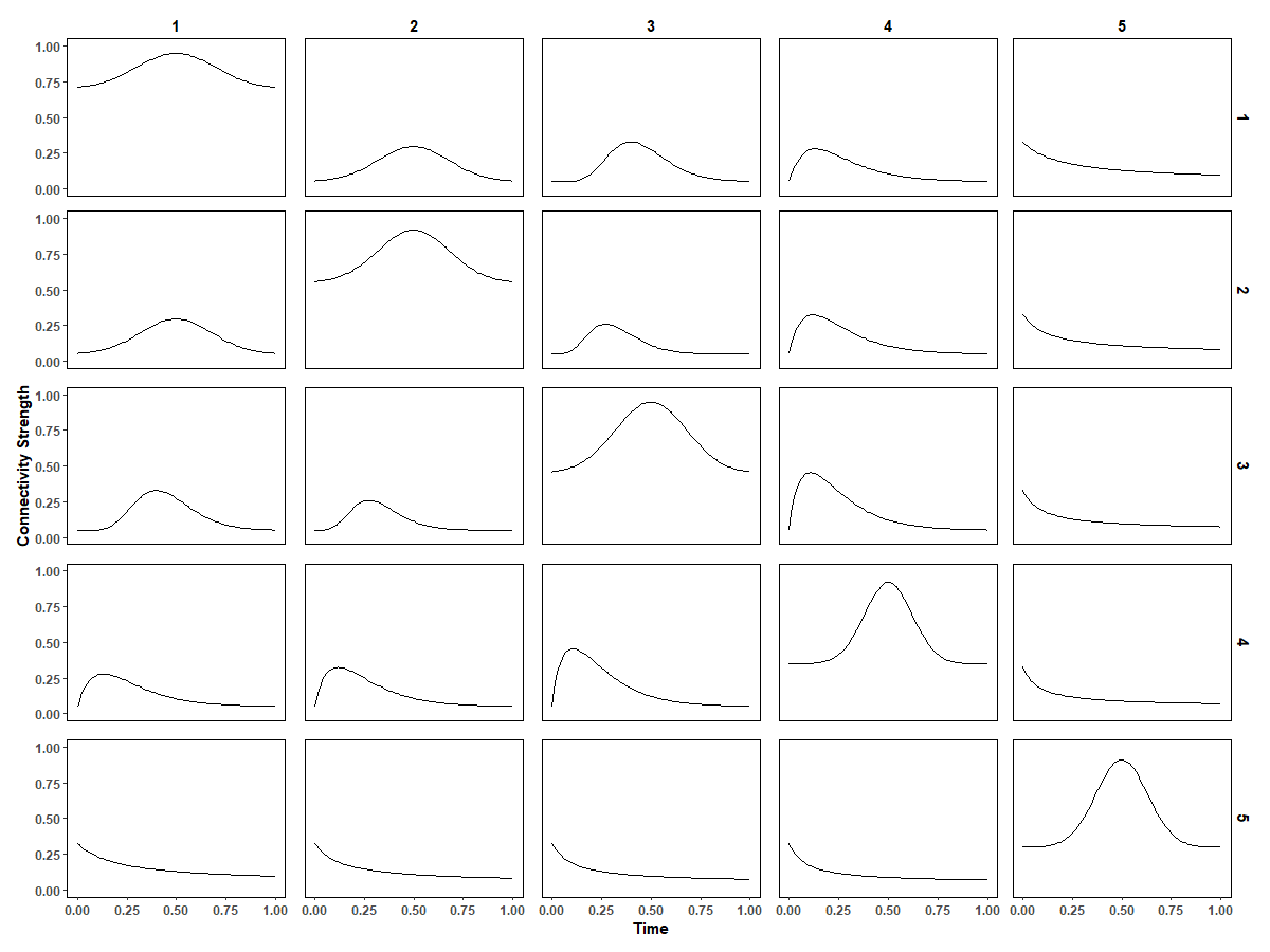
Figure S6: Time varying connectivity weights between the five communities $C_{1},\ldots,C_{5}$ for normal data.

Figure S7: Time varying connectivity weights between the five communities $C_{1},\ldots,C_{5}$ for generated outliers.

S11.2 Additional Figures in Case Study

References

- Ahidar-Coutrix et al., (2020) Ahidar-Coutrix, A., Le Gouic, T., and Paris, Q. (2020). Convergence rates for empirical barycenters in metric spaces: curvature, convexity and extendable geodesics. Probability Theory and Related Fields 177, 323–68.
- Arcones and Giné, (1993) Arcones, M. A. and Giné, E. (1993). Limit theorems for U-processes. Ann. Prob. 21, 1494–542.
- Bali and Boente, (2009) Bali, J. L. and Boente, G. (2009). Principal points and elliptical distributions from the multivariate setting to the functional case. Statistics & Probability Letters 79, 1858–65.
- Dai et al., (2021) Dai, X., Lin, Z., and Müller, H.-G. (2021). Modeling sparse longitudinal data on Riemannian manifolds. Biometrics 77,1328–41.
- Dai and Müller, (2018) Dai, X. and Müller, H.-G. (2018). Principal component analysis for functional data on Riemannian manifolds and spheres. Ann. Statist. 46, 3334–61.
- Dubey and Müller, (2020) Dubey, P. and Müller, H.-G. (2020). Functional models for time-varying random objects. J.R. Statist. Soc. B 82, 275–327.
- Dubey and Müller, (2021) Dubey, P. and Müller, H.-G. (2021). Modeling time-varying random objects and dynamic networks. J. Am. Statist. Assoc. 117, 2252–67.
- Gervini, (2008) Gervini, D. (2008). Robust functional estimation using the median and spherical principal components. Biometrika 95, 587–600.
- Han and Liu, (2018) Han, F. and Liu, H. (2018). ECA: High-dimensional elliptical component analysis in non-Gaussian distributions. J. Am. Statist. Assoc. 113, 252–68.
- Huber, (2004) Huber, P. J. (2004). Robust Statistics. New York: John Wiley.
- Hsing and Eubank, (2015) Hsing, T. and Eubank, R. (2015). Theoretical Foundations of Functional Data Analysis, with an Introduction to Linear Operators. New York: John Wiley.
- Kolar et al., (2010) Kolar, M., Song, L., Ahmed, A., and Xing, E. P. (2010). Estimating time-varying networks. Ann. Appl. Stat. 4, 94–123.
- Leyder et al., (2023) Leyder, S., Raymaekers, J., and Verdonck, T. (2023). Generalized spherical principal component analysis. arXiv preprint arXiv:2303.05836.
- Locantore et al., (1999) Locantore, N., Marron, J., Simpson, D., Tripoli, N., Zhang, J. and Cohen, K. (1999). Robust principal component analysis for functional data (with discussion). Test 8, 1–73.
- Marden, (1999) Marden, J. I. (1999). Some robust estimates of principal components. Statistics & Probability Letters, 43(4):349–359.
- Marron and Dryden, (2021) Marron, J.S. and Dryden, I.L. (2021). Object Oriented Data Analysis. New York: Chapman and Hall
- Petersen and Müller, (2019) Petersen, A. and Müller, H.-G. (2019). Fréchet regression for random objects with Euclidean predictors. Ann. Statist. 47, 691–719.
- Raymaekers and Rousseeuw, (2019) Raymaekers, J. and Rousseeuw, P. (2019). A generalized spatial sign covariance matrix. Journal of Multivariate Analysis, 171:94–111.
- Schiratti et al., (2015) Schiratti, J.-B., Allassonniere, S., Colliot, O., and Durrleman, S. (2015). Learning spatiotemporal trajectories from manifold-valued longitudinal data. Advances in Neural Information Processing Systems, 28.
- Shao et al., (2022) Shao, L., Lin, Z., and Yao, F. (2022). Intrinsic Riemannian functional data analysis for sparse longitudinal observations. Ann. Statist. 50, 1696–721.
- Sturm, (2003) Sturm, K.-T. (2003). Probability measures on metric spaces of nonpositive curvature. Heat Kernels and Analysis on Manifolds, Graphs, and Metric Spaces: Lecture Notes from a Quarter Program on Heat Kernels, Random Walks, and Analysis on Manifolds and Graphs: April 16-July 13, 2002, Emile Borel Centre of the Henri Poincaré Institute, Paris, France, 338–357.
- Taskinen et al., (2012) Taskinen, S., Koch, I., and Oja, H. (2012). Robustifying principal component analysis with spatial sign vectors. Statistics & Probability Letters 82, 765–774.
- van der Vaart and Wellner, (1996) van der Vaart, A. and Wellner, J. (1996). Weak Convergence of Empirical Processes: With Applications to Statistics. New York: Springer.
- Visuri et al., (2000) Visuri, S., Koivunen, V., and Oja, H. (2000). Sign and rank covariance matrices. Journal of Statistical Planning and Inference, 91(2):557–575.
- Wang et al., (2023) Wang, G., Liu, S., Han, F., and Di, C.-Z. (2023). Robust functional principal component analysis via a functional pairwise spatial sign operator. Biometrics 79, 1239–1253.
- Worsley et al., (2002) Worsley, K. J., Liao, C. H., Aston, J., Petre, V., Duncan, G., Morales, F., and Evans, A. C. (2002). A general statistical analysis for fMRI data. Neuroimage 15, 1–15.
- Zhong et al., (2022) Zhong, R., Liu, S., Li, H., and Zhang, J. (2022). Robust functional principal component analysis for non-Gaussian longitudinal data. Journal of Multivariate Analysis 189, 104864.

References

- Arcones and Giné, (1993) Arcones, M. A. and Giné, E. (1993). Limit theorems for U-processes. Ann. Prob. 21, 1494–542.
- Bosq, (2000) Bosq, D. (2000). Linear Processes in Function Spaces: Theory and Applications, volume 149. Springer Science & Business Media.
- Dubey and Müller, (2020) Dubey, P. and Müller, H.-G. (2020). Fréchet change-point detection. Ann. Statist., 48(6):3312–3335.
- Kosorok, (2008) Kosorok, M. R. (2008). Introduction to Empirical Processes and Semiparametric Inference. Springer.
- Petersen and Müller, (2019) Petersen, A. and Müller, H.-G. (2019). Fréchet regression for random objects with Euclidean predictors. Ann. Statist., 47(2):691–719.
- Severn et al., (2022) Severn, K. E., Dryden, I. L., and Preston, S. P. (2022). Manifold valued data analysis of samples of networks, with applications in corpus linguistics. Ann. Appl. Stat., 16(1):368–390.
- van der Vaart and Wellner, (1996) van der Vaart, A. and Wellner, J. (1996). Weak Convergence of Empirical Processes: With Applications to Statistics. New York: Springer.