Outcomes of Sub-Neptune Collisions

Abstract

Observed high multiplicity planetary systems are often tightly packed. Numerical studies indicate that such systems are susceptible to dynamical instabilities. Dynamical instabilities in close-in tightly packed systems, similar to those found in abundance by Kepler, often lead to planet-planet collisions. For sub-Neptunes, the dominant type of observed exoplanets, the planetary mass is concentrated in a rocky core, but the volume is dominated by a low-density gaseous envelope. For these, using the traditional ‘sticky-sphere’ assumption is questionable. Using both N-body integration and smoothed-particle hydrodynamics, we have simulated sub-Neptune collisions for a wide range in realistic kinematic properties such as impact parameters (${b^{\prime}}$) and impact velocities (${v_{\rm{im}}}$) to study the possible outcomes in detail. We find that the majority ($\sim 76\%$) of the collisions with kinematic properties similar to what is expected from dynamical instabilities in multiplanet systems may not lead to mergers of sub-Neptunes. Instead, the sub-Neptunes separate from each other, often with significant atmosphere loss. When mergers do occur, they can involve significant mass loss even from the core and can sometimes lead to complete disruption of one or both planets. Sub-Neptunes merge or disrupt if ${b^{\prime}}<{b_{\rm{c}}}$, a critical value dependent on ${v_{\rm{im}}}/{v_{\rm{esc}}}$, where ${v_{\rm{esc}}}$ is the escape velocity from the surface of the hypothetical merged planet assuming sticky-sphere. For ${v_{\rm{im}}}/{v_{\rm{esc}}}\lesssim 2.5$, ${b_{\rm{c}}}\propto({v_{\rm{im}}}/{v_{\rm{esc}}})^{-2}$, and collisions with ${b^{\prime}}<{b_{\rm{c}}}$ typically leads to mergers. On the other hand, for ${v_{\rm{im}}}/{v_{\rm{esc}}}\gtrsim 2.5$, ${b_{\rm{c}}}\propto{v_{\rm{im}}}/{v_{\rm{esc}}}$, and the collisions with ${b^{\prime}}<{b_{\rm{c}}}$ can result in complete destruction of one or both sub-Neptunes.

1 Introduction

In the last few decades, we have detected over $5,000$ exoplanets in more than $3,500$ planetary systems (NASA Exoplanet Archive, Akeson et al., 2013), revealing a diverse population of planets with little to no resemblance to the solar system. Among these, most abundant are the short-period ($<100$ days) super-Earths and sub-Neptunes, that have no solar system equivalent. Apart from the sheer number of planet discoveries, we now have a wealth of data on hundreds of multi-planet systems (e.g., Lissauer et al., 2011; Fabrycky et al., 2014). These systems are often dynamically packed and close to their stability limit (e.g., Deck et al., 2012; Fang & Margot, 2013). Numerous studies regarding the dynamical evolution and stability of such multi-planet systems have suggested that dynamical instabilities play a significant role in the final planet assembly and likely shaped the orbital architectures of planetary systems we observe today (e.g., Rasio & Ford, 1996; Chatterjee et al., 2008; Jurić & Tremaine, 2008; Pu & Wu, 2015; Volk & Gladman, 2015; Izidoro et al., 2017; Frelikh et al., 2019; Anderson et al., 2020; Goldberg & Batygin, 2022; Ghosh & Chatterjee, 2023).

Dynamical instability excites the planetary orbits which lead to close encounters between planets, eventually resulting in planet-planet collisions or ejections. In close-in planetary systems, planet-planet collisions are more common (e.g., Ghosh & Chatterjee, 2023). In these $N$-body dynamical models, the collisions are generally resolved using the ‘sticky-sphere’ approximation, where the colliding planets are merged into a single body, conserving mass and linear momentum. This simple approximation does not consider the detailed kinematics of different collisions and treats all collisions as perfect inelastic mergers, irrespective of the impact parameter and the relative velocity between the colliding bodies. In principle, depending on the kinematics of the specific collision, the planets may not always merge, such as in high-velocity collisions with impact parameters comparable to their radii. This situation is particularly relevant for sub-Neptune-type planets. The structure of these planets is such that most of the mass is concentrated in the core, while a low-density gaseous envelope constitutes most of its volume (e.g., Hadden & Lithwick, 2014; Lopez & Fortney, 2014; Weiss & Marcy, 2014; Rogers, 2015; Wolfgang & Lopez, 2015). Hence, the ‘sticky-sphere’ approximation, ubiquitous in $N$-body dynamical integrations, is questionable and may not be appropriate in many cases. Tackling these issues requires thorough numerical experiments involving proper three-dimensional multi-layered planet models and detailed hydrodynamic simulations of collisions between planets in a variety of collision scenarios.

Several studies of planetary collisions using numerical hydrodynamic simulations were conducted in the past, mainly focusing on the moon formation (e.g., Benz et al., 1986; Canup & Asphaug, 2001; Canup et al., 2013; Kegerreis et al., 2022) and effects of giant impacts on planets (e.g., Liu et al., 2015; Kegerreis et al., 2018, 2020b; Denman et al., 2020, 2022). In the context of addressing the deficiencies of the ‘sticky sphere’ approximation, Leinhardt & Stewart (2012) conducted simulations of collisions between rocky planetesimals, Hwang et al. (2017, 2018) studied highly grazing collisions of multi-layered sub-Neptune type planets, and Li et al. (2020) simulated close encounters between Jupiter-like planets.

In this study, we revisit the problem of sub-Neptune collisions. We use smoothed particle hydrodynamics (SPH, Gingold & Monaghan, 1977; Lucy, 1977) to make 3D models of differentiated, three-component planets and conduct detailed numerical experiments of planet-planet collisions, varying the initial conditions, to gain insight into the outcomes of such violent events. SPH is a widely used meshless hydrodynamic scheme, where the material is modeled by a finite number of fluid elements or ‘SPH particles’ (see Monaghan, 2005; Springel, 2010; Price, 2012, for reviews). While Hwang et al. (2018) were able to simulate grazing collisions of sub-Neptunes, where only the gaseous envelopes interact, our setup can simulate collisions of all possible impact parameters, including head-on collisions involving the planetary cores. This improvement is made possible by using appropriate equations of state (EOSs) for the planetary materials and a better treatment of SPH particles at the boundaries between core, mantle, and atmosphere (see subsection 2.2).

The rest of the paper is structured as follows. In section 2, we discuss the chosen initial conditions and describe the dynamical integrations to generate planet-planet collisions. We also present our numerical setup for creating 3D SPH planet models and performing the subsequent detailed hydrodynamic simulations of planet-planet collisions. In section 3, we present our key results. We summarise and conclude in section 4.

2 Numerical Setup

In this study, we consider two sub-Neptune planets with masses ${m_{\rm{1}}}=4.51M_{\earth}$, ${m_{\rm{2}}}=7.55M_{\earth}$ and radii ${r_{\rm{1}}}=3.56R_{\earth}$, ${r_{\rm{2}}}=3.69R_{\earth}$, orbiting around a $1.03M_{\sun}$ star. In our setup, we first initialize the planets in unstable orbits that would eventually lead to collisions. We use the pre-collision orbital properties to conduct detailed hydrodynamical simulations using SPH to determine the outcome of the collisions.

2.1 Pre-Collision Orbits

To generate planet-planet collisions, we create $N$-body models of the chosen planets in orbits around their host star. The inner planet’s semi-major axis is set to ${a_{\rm{1}}}=0.115{\rm{AU}}$. The outer planet is placed at a period ratio of $1.3$, corresponding to ${a_{\rm{2}}}=0.137{\rm{AU}}$. The planetary eccentricities ${e}$ are randomly chosen from a uniform distribution within $0<{e}<0.9$. The inclinations (${i}$) are randomly drawn from the Rayleigh distributions with $\bar{{i}}=0.024$ (Xie et al., 2016). We integrate these systems with the IAS15 integrator (Rein & Spiegel, 2015) implemented in the REBOUND (Rein & Liu, 2012) simulation package. A collision is considered when the distance between the planets is less than $({r_{\rm{1}}}+{r_{\rm{2}}})$. We stop the integrations whenever a collision is detected. Otherwise, we integrate till a predetermined stopping time ($\sim 16000$ years, $\gtrsim 4\times 10^{5}$ times the inner planet’s initial orbital period). In the event of a collision, we store a snapshot of the planetary orbits before the collision when the distance between the centres of mass for the planets is $5\times({r_{\rm{1}}}+{r_{\rm{2}}})$. These snapshots would later serve as the starting points of the SPH calculations. We run thousands of such systems to densely populate the parameter space in the impact parameters ($b$, the perpendicular distance between the velocity vectors of the two planets) and impact velocities (${v_{\rm{im}}}$) of planet-planet collisions. We measure $b$ and ${v_{\rm{im}}}$ when their surfaces make contact, i.e., the distance between the centres of mass of the planets is ${r_{\rm{1}}}+{r_{\rm{2}}}$. Throughout this work, we represent the impact parameter and impact velocity as dimensionless ratios ${b^{\prime}}\equiv b/({r_{\rm{1}}}+{r_{\rm{2}}})$ and ${v_{\rm{im}}}/{v_{\rm{esc}}}$ where, ${v_{\rm{esc}}}=\sqrt{2G({m_{\rm{1}}}+{m_{\rm{2}}})/{r^{\prime}}}$, $G$ is the gravitational constant, ${r^{\prime}}=({r_{\rm{1}}}^{3}+{r_{\rm{2}}}^{3})^{1/3}$ is the radius of a planet with mass ${m_{\rm{1}}}+{m_{\rm{2}}}$ and the same average density of the colliding planets. The parameter space explored in ${b^{\prime}}$ and ${v_{\rm{im}}}/{v_{\rm{esc}}}$ is motivated by the planet-planet scattering experiments conducted in Ghosh & Chatterjee (2023) (private communication) and summarized in Figure 1 and Table 2. Note that the planet-planet experiments described in Ghosh & Chatterjee (2023) involves sub-Neptunes of various sizes, whereas our study focuses on two specific sub-Neptunes. Despite this distinction, we believe that these collisions provide valuable insights into the potential parameter space.

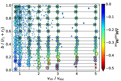
Figure 1: The 2D grid of simulations considered in our study in impact parameter (${b^{\prime}}\equiv b/({r_{\rm{1}}}+{r_{\rm{2}}})$) and impact velocity (${v_{\rm{im}}}$) at the moment of contact. The crosses represent the simulations conducted in this study. The colors of the individual crosses reflect the overall mass loss during the encounter. The blue (green) circles enclosing the crosses highlight the simulations where one (or both) planet(s) survive. Collisions resulting in the destruction of both planets are shown without any enclosing circle. The blue dots represent the collisions produced in typical planet-planet scattering experiments (ensemble n8-e040-i024 of Ghosh & Chatterjee (2023)). The dot sizes are proportional to the impact energy.

2.2 Hydrodynamic Simulations

Hydrodynamic simulations of planet-planet collisions were carried out using the SPH code StarSmasher (Rasio, 1991; Gaburov et al., 2010, 2018). This code implements an artificial viscosity prescription coupled with a Balsara Switch (Balsara, 1995) to avoid unphysical inter-particle penetration (described in Hwang et al., 2015). For our calculations, we use the Wendland C4 smoothing kernel (Wendland, 1995). We treat the host star as a non-interacting point-mass particle, exerting only gravitational influence over the planets. If a particle approaches within one solar radius of the star, it is accreted into the star, conserving mass and linear momentum.

We model the planets as differentiated bodies consisting of three layers - an iron core, a rocky mantle, and a hydrogen-helium (H-He) envelope. We implemented the widely used Tillotson (1962) iron and granite EOS (parameters are taken from Table A1 of Reinhardt & Stadel (2017)) to model the core and mantle materials respectively. For the H-He envelope, we use the Hubbard & Macfarlane (1980) EOS. In order to obtain the equilibrium planet profile, we utilize the code WoMa (Ruiz-Bonilla et al., 2020). We assume that $15\%$ of the total planet mass is in the H-He envelope, and the rest is in the iron core and rocky mantle in $30:70$ ratio. We truncate the planet profile at a negligible density of $0.01{{\rm g\ cm^{-3}}}$ and consider this as the planet’s surface. We fix the surface temperature (${T_{\rm{s}}}$) to our desired value depending on the insolation flux and assume an adiabatic temperature profile for the atmosphere. The core and the mantle are assumed to be isothermal. For simplicity, we assume that the planets have no initial spin. The parameters used to generate the equilibrium planet profiles including the outer radii of core (${r_{\rm{c}}}$), mantle (${r_{\rm{m}}}$), and the planet, and the pressure at the outermost surface layer (${P_{\rm{s}}}$) of the planets are provided in Table 1.

After obtaining the planet profiles, we place the SPH particles accordingly in concentric spherical shells using the stretched equal-area method (Kegerreis et al., 2019). The majority of the previous studies (e.g., Denman et al., 2020, 2022; Kegerreis et al., 2020b, a) have employed equal mass SPH particles with the most prominent exception of Hwang et al. (2017, 2018). However, opting for equal-mass SPH particles would lead to a concentration of most particles in the dense inner region of the planet, while the outer low-density H-He envelope, which constitutes most of the planet’s volume, would have a significantly lower resolution. We tackle this problem by utilizing StarSmasher’s ability to handle unequal mass particles (Gaburov et al., 2010) and setting the particle mass proportional to the density of its position inside the planet. This choice ensures a relatively uniform number density of SPH particles throughout the planet’s radial profile. Nevertheless, to prevent the accumulation of very low-mass particles in the outermost, least-dense layers, we limit the minimum mass for SPH particles to $1/1000$th of the most massive SPH particle. Our models have a resolution of $\sim 10^{5}$ particles per planet.

This SPH setup cannot yet be simulated because of the steep density discontinuities at the core-mantle and mantle-atmosphere boundaries. The sharp density discontinuities in the material boundaries can not be represented in the standard SPH framework because of the inherent smoothing of the density. Thus, if unaddressed, density-smoothing breaks the pressure continuity near these boundaries, resulting in high pressure gradients that lead to large artificial forces on the nearby SPH particles (Woolfson, 2007; Ruiz-Bonilla et al., 2022). Previous attempts to address this complication include changing the formulation of SPH (e.g., Price, 2008; Saitoh & Makino, 2013; Hosono et al., 2016), implementing corrections for the SPH density (e.g., Woolfson, 2007; Reinhardt et al., 2020; Ruiz-Bonilla et al., 2022) and using the so-called ”mixed composition” particles near the boundaries (e.g., Hwang et al., 2017, 2018). In our study, we adopt the prescription of mixed-composition particles outlined by Hwang et al. (2017). We replace the particles affected by density-smoothing with mixed composition particles. These particles are assumed to contain two different materials of different densities at pressure equilibrium with each other, such that the combined particle has the same density as the smoothed SPH density while conserving mass and preserving pressure continuity. For more details on the algorithms used to set up the mixed-composition particles, see Section A3 of Hwang et al. (2017), noting that we have updated the EOSs. These mixed composition particles are needed only to create stable SPH models of differentiated planets initially and have no role when they are outside the planet. Therefore, we allow these particles to revert to their initial pure compositions whenever these particles are outside a planet-like environment (when surrounding density is $<10^{-3}{{\rm g\ cm^{-3}}}$) at any point during the simulations to avoid complications in the pressure calculation algorithm specifically in very low-density regions.

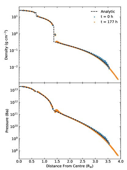
Figure 2: Density (upper panel) and pressure (lower panel) profiles of Planet-1 (Table 1). The black dashed line shows the analytic profile of the planet in hydrostatic equilibrium. The initial profiles of the SPH planet are shown in blue, and the same after relaxing the SPH planet in isolation for $177$ hours, is shown in orange.

Figure 2 shows the radial density and pressure profiles of Planet-1 as an example. Our SPH planet model is consistent with the analytic profile from WoMa even after the planet is relaxed in isolation for 177 hours, indicating that our SPH planet models are adequately stable. Note that there is some leakage of particles beyond the supplied outer edge of the planet during relaxation. This is likely related to the choice of the minimum density in the supplied planet profile. Had we chosen a lower density cutoff, the SPH density would have been even more consistent. Because the mass of this extended low-density layer is negligible, it is not expected to affect our simulations. The final snapshots from these relaxation runs are taken and initialized in pre-collision orbits obtained in subsection 2.1, around the point-mass host star. We now start our hydrodynamic simulation with both planets in a collision course and run it for a minimum duration of 44.3 hours. The eventual integration stopping time depends on the details of the collision and is discussed in subsection 2.4 and summarized in Table 2.

Table 1: Initial Planet Properties

Ensemble	${m}/M_{\earth}$	${r}/R_{\earth}$	${r_{\rm{c}}}/R_{\earth}$	${r_{\rm{m}}}/R_{\earth}$	${T_{\rm{s}}}/K$	${P_{\rm{s}}}/Ba$
Planet-1	$4.51$	$3.56$	$0.68$	$1.37$	$1091$	$4.15\times 10^{8}$
Planet-2	$7.55$	$3.69$	$0.75$	$1.51$	$1030$	$3.93\times 10^{8}$

Note. — Initial properties such as mass (${m}$), total radius (${r}$), outer radius of the core (${r_{\rm{c}}}$), outer radius of the mantle(${r_{\rm{m}}}$), surface temperature (${T_{\rm{s}}}$) and pressure (${P_{\rm{s}}}$) of the two planets considered in this study.

2.3 Identifying Post-Collision Planets

After conducting the hydrodynamic calculations, we are left with a distribution of fluid particles. However, this distribution does not immediately tell us the number of planets remaining in the simulation post-collision and which fluid particles constitute a planet. To identify the planetary bodies, we first use the DBSCAN (Ester et al., 1996) algorithm to identify clusters of core and mantle particles in the final snapshot of the hydrodynamic calculation. We treat these clusters as the initial planet candidates. Subsequently, we calculate the Jacobi constant for all the fluid particles corresponding to each of these planet candidates as (Murray & Dermott, 2000)

$$C_{\rm{J}}=\frac{x^{2}+y^{2}}{r^{2}}+\frac{2r}{{M_{\rm{*}}}+{m}}\left(\frac{{M_{\rm{*}}}}{{d_{\rm{1}}}}+\frac{{m}}{{d_{\rm{2}}}}\right)-\frac{rv^{2}}{G({M_{\rm{*}}}+{m})}$$ (1)

where ${M_{\rm{*}}}$ and ${m}$ are the masses of the host star and the planet candidate, $r$ is the distance between the star and planet candidate, ${d_{\rm{1}}}$ and ${d_{\rm{2}}}$ are the separations of the particle from the star and the planet candidate, ($x$, $y$) and $v$ represent the position co-ordinates and the velocity of the fluid particle in the co-rotating frame of the planet candidate and the star with origin at the center of mass. We then calculate the Jacobi constant at Lagrange point, ${L_{\rm{1}}}$ of the planet candidate, assuming a circular orbit (Murray & Dermott, 2000),

$$C_{{L_{\rm{1}}}}\approx 3+3^{4/3}\mu_{2}^{2/3}-10\mu_{2}/3$$ (2)

where $\mu_{2}={m}/({M_{\rm{*}}}+{m})$.

We assign the fluid particles to the planet candidate if they are located within the candidate’s Hill sphere and satisfy the criterion $C_{\rm{J}}>C_{{L_{\rm{1}}}}$. To ensure a reliable reconstruction of planetary bodies from these fluid particles, this process is iterated multiple times, updating the planet’s mass, position, and velocity in each iteration. Additionally, we exclude any planet candidates less massive than $0.1M_{\earth}$ to prevent misidentifying very small clusters of fluid particles as planets.

2.4 Determining Runtime of Simulations

After running the simulations for at least $44.3$ hours, we inspect the last snapshot and determine the number of planets still remaining in the simulation (see subsection 2.3 for details). If two planets remain with overlapping Hill spheres, we continue the simulation until their separation exceeds the combined size of their Hill spheres. This was needed for only one low ${v_{\rm{im}}}/{v_{\rm{esc}}}=0.78$ collision. Note that if we integrate such collisions further, there is a possibility that in their new orbits they might have another collision. However, in our framework, this would be considered a separate collision between planets with different initial structures and kinematics given by those of the collision remnants we have simulated. On the other hand, if only one planet survives, it may take a long time to settle, and our planet identification algorithm (subsection 2.3) may give us different masses if applied to snapshots taken at different times. As time progresses, the planet gradually stabilizes, and the results from the planet identification algorithm converge. We track this convergence using the difference in planet mass (${\Delta{m}}$) as calculated by our algorithm over time, and extend the simulation if necessary until ${|\Delta{m}/\Delta t|}$ falls below the threshold of $0.1\,M_{\earth}\rm{day}^{-1}$ or until we reach a predefined maximum duration of 332 hours (equivalent to the initial orbital period of the inner planet), imposed due to computational limitations. The chosen simulation stopping times for all the simulations are listed in Table 2. Note that for the majority of our simulations, ${|\Delta{m}/\Delta t|}$ is significantly below our specified threshold; the 16th percentile, median, and 84th percentiles for ${|\Delta{m}/\Delta t|}$ are $2.1\times 10^{-4}$, $4.1\times 10^{-3}$, and $3.5\times 10^{-2}$ $M_{\earth}\rm{day}^{-1}$, respectively.

3 Results

Figure 3: Snapshots showing the different stages of the encounter for the three major types of outcomes. In each panel, the reference frame is centered at the position of the most massive SPH particle, initially situated at the center of the more massive planet, and the colors represent the column density. The white arrows on the less massive planet represent its velocity relative to the more massive planet, with arrow length proportional to the velocity. The Hill spheres of the planets are shown by the white dashed circles on the rightmost panels. The top (middle) row shows an example of Hit & Run (Merger) encounter with ${v_{\rm{im}}}\sim{v_{\rm{esc}}}$ and ${b^{\prime}}=0.8$ (${b^{\prime}}=0.08$). The bottom row shows the snapshots of a highly energetic (${v_{\rm{im}}}/{v_{\rm{esc}}}\approx 4$) encounter with low impact parameter (${b^{\prime}}=0.05$) that results in the destruction of both the planets, categorized as a Catastrophic collision.

The outcomes of our collision simulations are summarized in Figure 1 and Table 2. We find that the outcomes of these collisions can be categorized into three major groups depending on the remaining number of planets, namely a) Hit & Run where both planets survive the encounter, b) Merger where the planets merge to form a single planet, and c) Catastrophic, violent collisions resulting in the destruction of one or both planets. Figure 3 shows examples of the time evolution of our hydrodynamic calculations, illustrating the different stages for each type of outcome.

As shown in Figure 4, our simulations achieve good energy conservation. The 16th percentile, median, and 84th percentile values for the relative energy error $|\Delta E/E|$ are $1.6\times 10^{-6}$, $3\times 10^{-6}$, and $2\times 10^{-5}$, respectively.

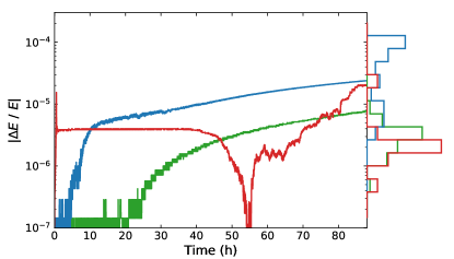
Figure 4: Relative energy error ($|\Delta E/E|$) throughout the runtime for three example collisions : ${b^{\prime}}=0.9$ at ${v_{\rm{im}}}/{v_{\rm{esc}}}\sim 0.78$ for Hit & Run (green), ${b^{\prime}}=0.14$ at ${v_{\rm{im}}}/{v_{\rm{esc}}}\sim 1$ representing a Merger (blue), and ${b^{\prime}}=0.19$ at ${v_{\rm{im}}}/{v_{\rm{esc}}}\sim 5$ depicting a Catastrophic collision. The marginalized histograms represent the distribution of $|\Delta E/E|$ at simulation stopping time.

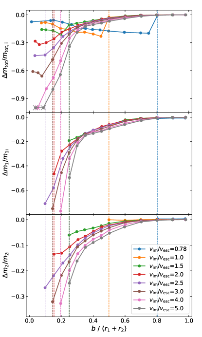
Figure 5: Fractional change in planet masses, against impact parameter for different impact velocities. The vertical dashed lines indicate the lowest impact parameters at which both planets survive for each ${v_{\rm{im}}}/{v_{\rm{esc}}}$ (see legend). Collisions resulting in the destruction of both planets are marked by crosses.

3.1 Hit & Run Collisions

In Hit & Run collisions, both planets survive the first contact with sufficient momentum to overcome their mutual gravitational attraction and go on their separate orbits (top panel, Figure 3). There is no immediate re-encounter before the next possible orbit crossing. When the impact velocity (${v_{\rm{im}}}/{v_{\rm{esc}}}\lesssim 1$) is low, the Hit & Run collisions occur at higher impact parameters (${b^{\prime}}\gtrsim 0.5$). During such encounters, the low-density H/He envelopes of the planets primarily interact, resulting in minimal mass loss predominantly from the gaseous envelopes. The fractional change in total planetary masses (${\Delta{m_{\rm{tot}}}/m_{\rm{tot,i}}}$, the subscript $\rm{i}$ denoting initial values), as well as the individual planetary masses (${\Delta{m_{\rm{1}}}/m_{\rm{1i}}}$, ${\Delta{m_{\rm{2}}}/m_{\rm{2i}}}$), and the fractional change in the gaseous envelopes (${\Delta m_{\rm{gas,tot}}/m_{\rm{gas,tot,i}}}$, ${\Delta m_{\rm{gas,1}}/m_{\rm{gas,1i}}}$ and ${\Delta m_{\rm{gas,2}}/m_{\rm{gas,2i}}}$) during the collisions with varying ${b^{\prime}}$ and ${v_{\rm{im}}}$, are shown in Figure 5 and Figure 6, respectively. As the ${v_{\rm{im}}}$ increases, the range of Hit & Run encounters expands to include lower impact parameters. When ${v_{\rm{im}}}$ exceeds ${v_{\rm{esc}}}$, the mantles of the planets may interact and still have enough momentum to escape their mutual gravitational attraction (e.g., ${b^{\prime}}\sim 0.2$ with ${v_{\rm{im}}}/{v_{\rm{esc}}}\sim 2$). As expected, with even higher impact velocities, encounters featuring even smaller impact parameters can lead to a Hit & Run collision and the mass loss increases as we increase ${v_{\rm{im}}}/{v_{\rm{esc}}}$ or decrease ${b^{\prime}}$ (see Figure 5). During highly energetic collisions with low ${b^{\prime}}$, substantial portions of the mantle layers and gaseous envelopes of both planets can erode, with the less massive planets being particularly susceptible. In some extreme cases, e.g., at ${b^{\prime}}=0.14$ with ${v_{\rm{im}}}/{v_{\rm{esc}}}\sim 3$, the lower mass planet can lose $\gtrsim 80\%$ of its mantle, while the more massive planet still retains $\gtrsim 70\%$ of its mantle. For some specific Hit & Run encounter (e.g., at $b\lesssim 0.35$ with ${v_{\rm{im}}}/{v_{\rm{esc}}}=1.5$), the higher mass planet can even steal some of the mantle material from the lower mass planet (see Table 2). Such energetic mantle-eroding collisions can potentially create the so-called ‘Super-Mercuries’ (e.g., Reinhardt et al., 2022). In general, the core of the planets remains relatively unaffected in Hit & Run encounters with high impact parameters (${b^{\prime}}\gtrsim 0.3$). However, for more energetic (${v_{\rm{im}}}/{v_{\rm{esc}}}\gtrsim 2$) encounters with lower impact parameters (${b^{\prime}}\lesssim 0.2$), the less massive planet can lose material from its core (see Table 2). In some cases, the massive planet can even capture a small portion of the lower mass planet’s core (e.g., at $b=0.1$ with ${v_{\rm{im}}}/{v_{\rm{esc}}}=2.5$) during the encounter.

3.2 Mergers

As the impact parameter decreases, the amount of mass involved in the interaction during the encounter increases, making it progressively harder for the planets to overcome each other’s gravitational pull. Consequently, this raises the probability of a Merger, where both the planets merge to form a single planet, more massive than either of the colliding planets. When the impact parameter and the impact velocity are sufficiently low, the planets collide nearly head-on and merge immediately, losing a small fraction of the total mass (e.g., ${\Delta{m_{\rm{tot}}}/m_{\rm{tot,i}}}=-0.09$ for a collision at ${b^{\prime}}=0.08$ with ${v_{\rm{im}}}/{v_{\rm{esc}}}\sim 1$, demonstrated in the middle panel of Figure 3). At greater impact velocities with comparable impact parameters, the degree of mass loss becomes more pronounced (e.g., ${\Delta{m_{\rm{tot}}}/m_{\rm{tot,i}}}=-0.32$ for a collision at ${b^{\prime}}=0.06$ with ${v_{\rm{im}}}/{v_{\rm{esc}}}\sim 2$). However, at higher impact parameters, the planets may not immediately merge during their initial close encounter. But, they also lack the necessary momentum to break free from each other’s gravitational attraction, as in Hit & Run encounters. After the first encounter, they return for one or more subsequent close encounters and eventually merge (e.g., the collision at ${b^{\prime}}=0.4$ with ${v_{\rm{im}}}/{v_{\rm{esc}}}\sim 1$). This violent path to their eventual merger via multiple close approaches creates greater churning and results in a substantial mass loss (up to $23\%$ for ${v_{\rm{im}}}/{v_{\rm{esc}}}\lesssim 1.5$) in such events (see Figure 5 and Table 2). Due to the repetitive nature of these encounters, it was necessary to extend these simulations beyond our typical stopping time, as detailed in subsection 2.4.

Because of these increased mass loss in such collisions, the ${\Delta{m_{\rm{tot}}}/m_{\rm{tot,i}}}$ versus ${b^{\prime}}$ curve shows a notable drop near the boundary between the Hit & Run and Merger regimes (Figure 5). For lower values of ${b^{\prime}}$, the collision smoothly transitions toward head-on Mergers, and the amount of mass lost during the encounters decreases. During Merger encounters with ${v_{\rm{im}}}/{v_{\rm{esc}}}\lesssim 2$, the collision remnant can retain the entire core material from the colliding planets, with the mass loss occurring solely from their mantles and gaseous envelopes. In such scenarios, it is possible for up to approximately $\sim 30\%$ of the total mantle material to be stripped away along with the complete removal of their gaseous envelopes (e.g., at ${b^{\prime}}=0.06$ with ${v_{\rm{im}}}/{v_{\rm{esc}}}\sim 2$). The fractional change in the total gas mass (${\Delta m_{\rm{gas,tot}}/m_{\rm{gas,tot,i}}}$) during these Merger events shows an interesting trend. For relatively larger ${b^{\prime}}$, particularly near the boundary between the Hit & Run and Merger outcomes, where it takes repeated encounters for the planets to merge, the collision remnant cannot hold on to the atmosphere from the colliding bodies, resulting in a rocky collision product with no significant gaseous envelope. However, with lower impact parameters, the number of encounters needed to complete the merger reduces. Consequently, the collision remnant can retain substantial amounts of the atmospheres (up to $\sim 60\%$, e.g., at ${b^{\prime}}=0.15$ with ${v_{\rm{im}}}/{v_{\rm{esc}}}=0.78$) from the parent bodies. The lower the impact velocity, the higher the amount of the atmosphere retained by the merger product. This shift and reversal in trends in both the ${\Delta{m_{\rm{tot}}}/m_{\rm{tot,i}}}$ versus ${b^{\prime}}$ curve (Figure 5) and the ${\Delta m_{\rm{gas,tot}}/m_{\rm{gas,tot,i}}}$ versus ${b^{\prime}}$ curve (Figure 6) are particularly prominent when ${v_{\rm{im}}}/{v_{\rm{esc}}}\lesssim 1.5$.

3.3 Catastrophic Collisions

At high impact velocities (${v_{\rm{im}}}/{v_{\rm{esc}}}\gtrsim 2.5$), collisions with low impact parameters (${b^{\prime}}\lesssim 0.2$) can be highly destructive. Such high impact velocity collisions involve significant energy capable of ejecting substantial portions of the initially bound planetary mass beyond the gravitational influence of the collision remnant. In the aftermath of such collisions, if only one planetary body remains or none at all, and the total mass loss exceeds the initial mass of one of the colliding planets, signifying that the collision essentially destroyed one or both of them, we categorize the encounter as a Catastrophic collision . When a planetary body manages to survive such a highly destructive event, it can only retain a small portion of the combined mass from the colliding bodies. This results in significant loss of core and mantle materials and the complete depletion of the gaseous envelope that the parent bodies once had. In certain instances, the surviving body may consist of $\sim 50\%$ ($\sim 10\%$) of the combined initial core (mantle) material of the parent bodies (e.g., at ${b^{\prime}}=0.15$ with ${v_{\rm{im}}}/{v_{\rm{esc}}}\sim 5$). In some extreme scenarios, such as at ${b^{\prime}}\lesssim 0.05$ with ${v_{\rm{im}}}/{v_{\rm{esc}}}\sim 4$ (bottom panel, Figure 3) or at ${b^{\prime}}\lesssim 0.1$ with ${v_{\rm{im}}}/{v_{\rm{esc}}}\sim 5$, both parent planets disintegrate entirely, and the material that once was part of these planets starts orbiting the host star as debris.

Note that such exotic collisions between planetary bodies are exceptionally rare in typical simulations of dynamical instabilities that are expected to occur during the final stage of planet assembly; only one out of $1,094$ collisions in the ensemble n8-e040-i024 of Ghosh & Chatterjee (2023) falls under this category (private communication).

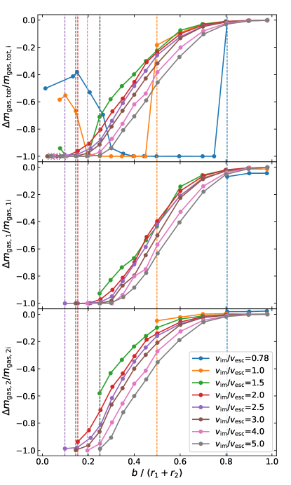
Figure 6: Similar to Figure 5 but shows fractional change in the atmospheric mass of the planets with varying ${b^{\prime}}$ for different values of ${v_{\rm{im}}}/{v_{\rm{esc}}}$.

3.4 Boundaries Between Different Outcomes as a Function of ${b^{\prime}}$ and ${v_{\rm{im}}}/{v_{\rm{esc}}}$

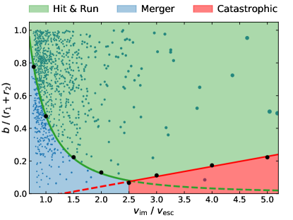
Figure 7: Summary of overall outcomes in ${b^{\prime}}-{v_{\rm{im}}}$ space. The black dots mark the ${b_{\rm{c}}}$ values from our simulation grid. The boundary separating Hit & Run collisions with other outcomes, follows ${b_{\rm{c}}}/{b_{\rm{c,1}}}\approx({v_{\rm{im}}}/{v_{\rm{esc}}})^{-2}$, for ${v_{\rm{im}}}/{v_{\rm{esc}}}\lesssim 2.5$ and ${b_{\rm{c}}}$ increases linearly (${b_{\rm{c}}}/{b_{\rm{c,2.5}}}\approx({v_{\rm{im}}}/{v_{\rm{esc}}})-1.5$) at higher impact velocities. Similar to Figure 1, the blue dots represent the collisions produced in typical planet-planet scattering experiments (ensemble n8-e040-i024 of Ghosh & Chatterjee (2023)).

In this section, we closely examine the boundaries between different outcomes in the ${b^{\prime}}-{v_{\rm{im}}}$ space. The three major regimes in the ${b^{\prime}}-{v_{\rm{im}}}/{v_{\rm{esc}}}$ space are summarized in Figure 7. We first examine the critical value, ${b_{\rm{c}}}$ of ${b^{\prime}}$ separating the Hit & Run encounters with others for the different values of ${v_{\rm{im}}}/{v_{\rm{esc}}}$. In our discrete grid, we estimate ${b_{\rm{c}}}$ as the midpoint between the adjacent two grid points where the outcome transitions for a given ${v_{\rm{im}}}/{v_{\rm{esc}}}$. As expected, ${b_{\rm{c}}}$ depends on ${v_{\rm{im}}}$. In general, lower ${v_{\rm{im}}}$ leads to higher ${b_{\rm{c}}}$. For example, in the collisions with ${v_{\rm{im}}}/{v_{\rm{esc}}}=0.78$, we find ${b_{\rm{c}}}=0.78$, that is, all encounters with ${v_{\rm{im}}}<0.78$, lead to the merger of the two planets. On the other hand, for ${v_{\rm{im}}}/{v_{\rm{esc}}}=2$, ${b_{\rm{c}}}=0.13$.

For ${v_{\rm{im}}}/{v_{\rm{esc}}}\lesssim 2.5$, we find that the dependency of ${b_{\rm{c}}}$ on ${v_{\rm{im}}}/{v_{\rm{esc}}}$ approximately follows ${b_{\rm{c}}}={b_{\rm{c,1}}}\times({v_{\rm{im}}}/{v_{\rm{esc}}})^{-2}$, where ${b_{\rm{c,1}}}=0.474\pm 0.025$ is the value of ${b_{\rm{c}}}$ at ${v_{\rm{im}}}/{v_{\rm{esc}}}=1$. The errors indicate the spacing between our discrete grid points near ${b_{\rm{c}}}$. In other words ${b_{\rm{c}}}$ is inversely proportional to the impact energy (${E_{\rm{im}}}=\frac{1}{2}\mu{v_{\rm{im}}}^{2}$, where $\mu=\frac{{m_{\rm{1}}}{m_{\rm{2}}}}{{m_{\rm{1}}}+{m_{\rm{2}}}}$, the reduced mass of the two planet system). This dependency arises since, at lower impact speeds or equivalently lower energies, the planets do not have enough energy to escape their mutual gravitational potential well, even at higher impact parameters, ultimately resulting in Mergers. Conversely, as the impact energy increases, the planets can penetrate more deeply into their gravitational potential well and still escape, resulting in lower ${b_{\rm{c}}}$ for higher ${v_{\rm{im}}}$. Interestingly, for the planets considered in our study, we find ${b_{\rm{c,1}}}\approx 1.2\times({r_{\rm{c}}}_{\rm{1}}+{r_{\rm{c}}}_{\rm{2}})$. It would be interesting to investigate whether this relationship holds for planets with different structures and initial properties in future studies.

Around ${v_{\rm{im}}}/{v_{\rm{esc}}}\approx 2.5$, ${b_{\rm{c}}}$ decreases significantly and reaches ${b_{\rm{c,2.5}}}=0.07$, equivalent to $\approx({r_{\rm{c}}}_{\rm{1}}+{r_{\rm{c}}}_{\rm{2}})/6$. In such high ${v_{\rm{im}}}$ collisions at low ${b^{\prime}}$ ($\lesssim{b_{\rm{c}}}$), the outcome is typically a Catastrophic collision. Beyond ${v_{\rm{im}}}/{v_{\rm{esc}}}\approx 2.5$, ${b_{\rm{c}}}$ no longer decreases with increasing ${v_{\rm{im}}}$. Instead ${b_{\rm{c}}}$ exhibits a linear increase with ${v_{\rm{im}}}$: ${b_{\rm{c}}}/{b_{\rm{c,2.5}}}\approx({v_{\rm{im}}}/{v_{\rm{esc}}})-1.5$. In this regime, ${b_{\rm{c}}}$ is so low that significant portions of the mantle and the core are involved in encounters with ${b^{\prime}}\approx{b_{\rm{c}}}$. At lower energies just above ${b_{\rm{c}}}$, despite significant perturbation of the inner planetary layers, both planets can still hold on to their mass and survive the encounter, resulting in a Hit & Run encounter (e.g., at ${b^{\prime}}=0.14$ with ${v_{\rm{im}}}/{v_{\rm{esc}}}\sim 3$). However, at the same $b$ at a higher impact velocity (e.g., at ${b^{\prime}}=0.15$ with ${v_{\rm{im}}}/{v_{\rm{esc}}}\sim 4$), the increased energy of the impact causes the less massive planet to disintegrate entirely, ultimately resulting in only one survivor. Consequently, ${b_{\rm{c}}}$ increases with ${v_{\rm{im}}}/{v_{\rm{esc}}}$.

4 Summary And Discussions

In this study, we present our numerical framework to study sub-Neptune collisions using a combination of $N$-body, planet structure, and SPH simulations. We have applied our setup to conduct $123$ hydrodynamical simulations of collisions between two specific sub-Neptune planets for various impact parameters and impact velocities expected during dynamical instabilities. Our key results are summarized below.

• There are three different outcomes, namely a) Hit & Run in which both planets survive the grazing encounter, b) Mergers, forming a single planet, more massive than the individual colliding planets, and c) Catastrophic collisions, resulting in the effective destruction of one or both planets.

• Hit & Run encounters are the most common, spanning the most substantial region in the ${b^{\prime}}-{v_{\rm{im}}}$ space (Figure 7), among the three. Such collisions occur at relatively larger impact parameters at lower impact velocities, where only the low-density gaseous envelopes interact. As impact velocities increase, these encounters extend to smaller ${b^{\prime}}$. The higher the impact velocity or lower the impact parameter, the greater the amount of mass lost during the encounter.

• At lower impact parameters, the planets cannot overcome their mutual gravitational pull, resulting in a Merger, where they form a single massive planet, losing a small fraction of the total mass of the colliding planets. At relatively higher impact parameters, the planets may survive the initial encounter. However, without sufficient energy to overcome their gravitational attraction, they would return immediately for one or more close encounters and eventually merge with more substantial mass loss.

• At large impact velocities (${v_{\rm{im}}}/{v_{\rm{esc}}}\gtrsim 2.5$), the low-${b^{\prime}}$ collisions can be highly destructive (red shaded region, Figure 7), effectively disintegrating one or, in some extreme cases, both planets. These collisions are referred to as Catastrophic collisions.

• The critical impact parameter (${b_{\rm{c}}}$) separating the Hit & Run and Merger encounters, depends on ${v_{\rm{im}}}$ or equivalently the impact energy ${E_{\rm{im}}}$. We find that for ${v_{\rm{im}}}/{v_{\rm{esc}}}\lesssim 2.5$, ${b_{\rm{c}}}\propto({v_{\rm{im}}}/{v_{\rm{esc}}})^{-2}\sim{E_{\rm{im}}}^{-1}$. In other words, as the planets get closer, they require more energy to overcome their gravitational attraction. For ${v_{\rm{im}}}/{v_{\rm{esc}}}\gtrsim 2.5$, ${b_{\rm{c}}}$ separates the Hit & Run and Catastrophic encounters. In this regime, ${b_{\rm{c}}}$ increases linearly with (${v_{\rm{im}}}/{v_{\rm{esc}}}$) as the increased impact energy disintegrates the lower mass planet more efficiently.

• Interestingly, we find that the majority of the collisions ($\approx 76\%$) that were treated as perfect mergers in Ghosh & Chatterjee (2023) may fall within the Hit & Run regime if the collisions involve sub-Neptunes with substantial gaseous envelopes. Even those falling under the Mergers regime, the remnants can lose a significant amount of mass and atmosphere and hence can not be treated as perfect mergers.

A more detailed future study with a multi-dimensional grid with the initial planet masses and atmospheric fractions as input parameters would shed more light on the outcomes of the sub-Neptune collisions. Such a study would provide insights into the amount of mass loss and atmospheric depletion in such encounters for a wider range in parameter space. The development of an analytic prescription based on these results could be of great use to enable us treat collisions more realistically in $N$-body modeling of planetary systems. It would be particularly interesting to assess the impact of accurate collision modeling on the outcomes of $N$-body dynamical evolution studies of exoplanets, such as Ghosh & Chatterjee (2023). This work is the first step towards this goal.

Table 2: Summarized results of all the simulations conducted in this study.

Number	$v_{\rm{im}}/v_{\rm{esc}}$	$b\ /\ (r_{1}+r_{2})$	$t_{\rm{stop}}/\rm{hour}$	Outcome	$m$	$\Delta m/m_{\rm{i}}$	$\Delta m_{\rm{core}}/m_{\rm{core,i}}$	$\Delta m_{\rm{mantle}}/m_{\rm{mantle,i}}$	$\Delta m_{\rm{gas}}/m_{\rm{gas,i}}$
1	$0.78$	$0.01$	$44.3$	MG	$11.14$	$-0.08$	$0.00$	$0.00$	$-0.50$
2	$0.77$	$0.13$	$44.3$	MG	$11.30$	$-0.06$	$0.00$	$0.00$	$-0.41$
3	$0.78$	$0.15$	$44.3$	MG	$11.36$	$-0.06$	$0.00$	$0.00$	$-0.38$
4	$0.76$	$0.21$	$132.8$	MG	$11.08$	$-0.08$	$0.00$	$0.00$	$-0.53$
5	$0.76$	$0.26$	$177.1$	MG	$10.79$	$-0.10$	$0.00$	$0.00$	$-0.69$
6	$0.78$	$0.30$	$177.1$	MG	$10.35$	$-0.14$	$0.00$	$0.00$	$-0.94$
7	$0.77$	$0.35$	$177.1$	MG	$10.27$	$-0.15$	$0.00$	$0.00$	$-0.98$
8	$0.77$	$0.40$	$265.6$	MG	$10.13$	$-0.16$	$0.00$	$-0.01$	$-1.00$
9	$0.77$	$0.44$	$265.6$	MG	$10.08$	$-0.16$	$0.00$	$-0.02$	$-1.00$
10	$0.76$	$0.50$	$332.0$	MG	$9.94$	$-0.17$	$0.00$	$-0.04$	$-1.00$
11	$0.78$	$0.60$	$332.0$	MG	$9.78$	$-0.19$	$0.00$	$-0.06$	$-1.00$
12	$0.78$	$0.70$	$332.0$	MG	$9.70$	$-0.19$	$0.00$	$-0.08$	$-1.00$
13	$0.77$	$0.75$	$332.0$	MG	$9.66$	$-0.20$	$0.00$	$-0.08$	$-1.00$
14	$0.78$	$0.80$	$44.3$	HR	$4.46,\ 7.56$	$-0.01,\ 0.00$	$0.00,\ 0.00$	$0.00,\ 0.00$	$-0.07,\ 0.02$
15	$0.78$	$0.90$	$88.5$	HR	$4.47,\ 7.56$	$-0.01,\ 0.00$	$0.00,\ 0.00$	$0.00,\ 0.00$	$-0.04,\ 0.02$
16	$0.78$	$0.98$	$44.3$	HR	$4.47,\ 7.57$	$-0.01,\ 0.00$	$0.00,\ 0.00$	$0.00,\ 0.00$	$-0.04,\ 0.02$
17	$0.99$	$0.08$	$44.3$	MG	$10.99$	$-0.09$	$0.00$	$0.00$	$-0.58$
18	$0.98$	$0.10$	$44.3$	MG	$11.05$	$-0.08$	$0.00$	$0.00$	$-0.55$
19	$1.00$	$0.14$	$88.5$	MG	$10.84$	$-0.10$	$0.00$	$-0.00$	$-0.67$
20	$1.04$	$0.20$	$221.3$	MG	$10.27$	$-0.15$	$0.00$	$0.00$	$-0.98$
21	$0.98$	$0.25$	$265.6$	MG	$10.13$	$-0.16$	$0.00$	$-0.01$	$-1.00$
22	$1.02$	$0.30$	$332.0$	MG	$9.77$	$-0.19$	$0.00$	$-0.06$	$-1.00$
23	$1.01$	$0.35$	$332.0$	MG	$9.80$	$-0.19$	$0.00$	$-0.06$	$-1.00$
24	$0.97$	$0.40$	$332.0$	MG	$9.56$	$-0.21$	$0.00$	$-0.09$	$-1.00$
25	$1.00$	$0.45$	$332.0$	MG	$9.26$	$-0.23$	$-0.00$	$-0.14$	$-1.00$
26	$1.00$	$0.50$	$44.3$	HR	$4.18,\ 7.54$	$-0.07,\ -0.00$	$0.00,\ 0.00$	$-0.02,\ 0.01$	$-0.41,\ -0.05$
27	$1.04$	$0.60$	$44.3$	HR	$4.35,\ 7.52$	$-0.03,\ -0.00$	$0.00,\ 0.00$	$-0.00,\ 0.00$	$-0.21,\ -0.02$
28	$1.03$	$0.70$	$44.3$	HR	$4.45,\ 7.54$	$-0.01,\ 0.00$	$0.00,\ 0.00$	$0.00,\ 0.00$	$-0.08,\ 0.00$
29	$1.02$	$0.80$	$44.3$	HR	$4.48,\ 7.54$	$-0.00,\ 0.00$	$0.00,\ 0.00$	$0.00,\ 0.00$	$-0.03,\ 0.00$
30	$1.04$	$0.90$	$44.3$	HR	$4.49,\ 7.54$	$-0.00,\ 0.00$	$0.00,\ 0.00$	$0.00,\ 0.00$	$-0.01,\ 0.00$
31	$0.95$	$0.98$	$44.3$	HR	$4.49,\ 7.54$	$-0.00,\ 0.00$	$0.00,\ 0.00$	$0.00,\ 0.00$	$-0.01,\ 0.00$
32	$1.48$	$0.08$	$88.5$	MG	$10.13$	$-0.16$	$0.00$	$-0.03$	$-0.94$
33	$1.46$	$0.10$	$177.1$	MG	$10.10$	$-0.16$	$0.00$	$-0.02$	$-1.00$
34	$1.47$	$0.15$	$177.1$	MG	$10.02$	$-0.17$	$0.00$	$-0.03$	$-1.00$
35	$1.53$	$0.20$	$265.6$	MG	$9.50$	$-0.21$	$0.00$	$-0.10$	$-1.00$
36	$1.51$	$0.25$	$44.3$	HR	$3.64,\ 7.09$	$-0.19,\ -0.06$	$-0.02,\ 0.01$	$-0.08,\ 0.04$	$-0.93,\ -0.58$
37	$1.49$	$0.30$	$44.3$	HR	$3.75,\ 7.19$	$-0.17,\ -0.05$	$0.00,\ 0.00$	$-0.07,\ 0.03$	$-0.83,\ -0.43$
38	$1.46$	$0.35$	$44.3$	HR	$3.89,\ 7.24$	$-0.14,\ -0.04$	$0.00,\ 0.00$	$-0.04,\ 0.02$	$-0.74,\ -0.33$
39	$1.50$	$0.40$	$44.3$	HR	$4.02,\ 7.29$	$-0.11,\ -0.03$	$0.00,\ 0.00$	$-0.01,\ 0.00$	$-0.67,\ -0.24$
40	$1.54$	$0.45$	$44.3$	HR	$4.14,\ 7.36$	$-0.08,\ -0.02$	$0.00,\ 0.00$	$0.00,\ 0.00$	$-0.54,\ -0.16$
41	$1.48$	$0.50$	$44.3$	HR	$4.21,\ 7.43$	$-0.07,\ -0.01$	$0.00,\ 0.00$	$0.00,\ 0.00$	$-0.43,\ -0.10$
42	$1.50$	$0.60$	$44.3$	HR	$4.41,\ 7.50$	$-0.02,\ -0.01$	$0.00,\ 0.00$	$0.00,\ 0.00$	$-0.14,\ -0.04$
43	$1.54$	$0.70$	$44.3$	HR	$4.46,\ 7.52$	$-0.01,\ -0.00$	$0.00,\ 0.00$	$0.00,\ 0.00$	$-0.06,\ -0.01$
44	$1.53$	$0.80$	$44.3$	HR	$4.49,\ 7.53$	$-0.00,\ -0.00$	$0.00,\ 0.00$	$0.00,\ 0.00$	$-0.02,\ -0.00$
45	$1.49$	$0.90$	$44.3$	HR	$4.50,\ 7.54$	$-0.00,\ -0.00$	$0.00,\ 0.00$	$0.00,\ 0.00$	$-0.01,\ -0.00$
46	$1.49$	$0.98$	$44.3$	HR	$4.50,\ 7.54$	$-0.00,\ -0.00$	$0.00,\ 0.00$	$0.00,\ 0.00$	$-0.00,\ -0.00$
47	$1.99$	$0.04$	$88.5$	MG	$8.62$	$-0.28$	$0.00$	$-0.23$	$-1.00$
48	$2.04$	$0.06$	$88.5$	MG	$8.18$	$-0.32$	$-0.00$	$-0.29$	$-1.00$
49	$2.02$	$0.10$	$88.5$	MG	$8.44$	$-0.30$	$0.00$	$-0.25$	$-1.00$
50	$1.98$	$0.15$	$44.3$	HR	$2.41,\ 6.52$	$-0.47,\ -0.13$	$-0.10,\ 0.05$	$-0.49,\ -0.01$	$-1.00,\ -0.94$
51	$2.01$	$0.20$	$44.3$	HR	$3.25,\ 6.55$	$-0.28,\ -0.13$	$-0.03,\ 0.01$	$-0.20,\ -0.01$	$-1.00,\ -0.85$
52	$1.97$	$0.25$	$44.3$	HR	$3.49,\ 6.74$	$-0.23,\ -0.11$	$-0.01,\ 0.00$	$-0.13,\ -0.00$	$-0.97,\ -0.70$
53	$1.97$	$0.30$	$44.3$	HR	$3.73,\ 6.95$	$-0.17,\ -0.08$	$0.00,\ 0.00$	$-0.06,\ 0.00$	$-0.90,\ -0.53$
54	$2.04$	$0.35$	$44.3$	HR	$3.89,\ 7.05$	$-0.14,\ -0.06$	$0.00,\ 0.00$	$-0.02,\ 0.00$	$-0.81,\ -0.44$
55	$1.99$	$0.40$	$44.3$	HR	$4.02,\ 7.19$	$-0.11,\ -0.05$	$0.00,\ 0.00$	$-0.00,\ 0.00$	$-0.70,\ -0.31$
56	$2.02$	$0.45$	$44.3$	HR	$4.16,\ 7.33$	$-0.08,\ -0.03$	$0.00,\ 0.00$	$0.00,\ 0.00$	$-0.51,\ -0.19$
57	$2.00$	$0.50$	$44.3$	HR	$4.23,\ 7.38$	$-0.06,\ -0.02$	$0.00,\ 0.00$	$0.00,\ 0.00$	$-0.40,\ -0.14$
58	$2.02$	$0.60$	$44.3$	HR	$4.39,\ 7.47$	$-0.03,\ -0.01$	$0.00,\ 0.00$	$0.00,\ 0.00$	$-0.17,\ -0.06$
59	$2.04$	$0.70$	$44.3$	HR	$4.46,\ 7.52$	$-0.01,\ -0.00$	$0.00,\ 0.00$	$0.00,\ 0.00$	$-0.06,\ -0.02$
60	$1.96$	$0.80$	$44.3$	HR	$4.49,\ 7.53$	$-0.00,\ -0.00$	$0.00,\ 0.00$	$0.00,\ 0.00$	$-0.02,\ -0.00$
61	$2.00$	$0.90$	$44.3$	HR	$4.50,\ 7.54$	$-0.00,\ -0.00$	$0.00,\ 0.00$	$0.00,\ 0.00$	$-0.00,\ -0.00$
62	$2.04$	$0.98$	$44.3$	HR	$4.50,\ 7.54$	$-0.00,\ -0.00$	$0.00,\ 0.00$	$0.00,\ 0.00$	$-0.00,\ -0.00$
63	$2.46$	$0.03$	$44.3$	CC	$6.76$	$-0.44$	$-0.04$	$-0.47$	$-1.00$
64	$2.54$	$0.10$	$44.3$	HR	$1.31,\ 5.53$	$-0.71,\ -0.27$	$-0.39,\ 0.12$	$-0.77,\ -0.25$	$-1.00,\ -0.99$
65	$2.52$	$0.15$	$44.3$	HR	$1.89,\ 5.88$	$-0.58,\ -0.22$	$-0.14,\ 0.02$	$-0.66,\ -0.13$	$-1.00,\ -0.98$
66	$2.50$	$0.21$	$44.3$	HR	$2.98,\ 6.26$	$-0.34,\ -0.17$	$-0.04,\ 0.00$	$-0.30,\ -0.06$	$-1.00,\ -0.91$
67	$2.52$	$0.25$	$44.3$	HR	$3.40,\ 6.50$	$-0.24,\ -0.14$	$0.00,\ 0.00$	$-0.16,\ -0.03$	$-0.99,\ -0.81$
68	$2.51$	$0.30$	$44.3$	HR	$3.70,\ 6.80$	$-0.18,\ -0.10$	$0.00,\ 0.00$	$-0.06,\ -0.01$	$-0.95,\ -0.62$
69	$2.51$	$0.35$	$44.3$	HR	$3.91,\ 7.00$	$-0.13,\ -0.07$	$0.00,\ 0.00$	$-0.01,\ -0.00$	$-0.84,\ -0.47$
70	$2.49$	$0.40$	$44.3$	HR	$4.02,\ 7.15$	$-0.11,\ -0.05$	$0.00,\ 0.00$	$0.00,\ 0.00$	$-0.71,\ -0.35$
71	$2.52$	$0.45$	$44.3$	HR	$4.11,\ 7.26$	$-0.09,\ -0.04$	$0.00,\ 0.00$	$0.00,\ 0.00$	$-0.59,\ -0.24$
72	$2.52$	$0.50$	$44.3$	HR	$4.22,\ 7.36$	$-0.06,\ -0.02$	$0.00,\ 0.00$	$0.00,\ 0.00$	$-0.42,\ -0.16$
73	$2.50$	$0.60$	$44.3$	HR	$4.36,\ 7.46$	$-0.03,\ -0.01$	$0.00,\ 0.00$	$0.00,\ 0.00$	$-0.21,\ -0.07$
74	$2.47$	$0.70$	$44.3$	HR	$4.45,\ 7.51$	$-0.01,\ -0.00$	$0.00,\ 0.00$	$0.00,\ 0.00$	$-0.08,\ -0.02$
75	$2.47$	$0.80$	$44.3$	HR	$4.49,\ 7.53$	$-0.00,\ -0.00$	$0.00,\ 0.00$	$0.00,\ 0.00$	$-0.02,\ -0.01$
76	$2.52$	$0.90$	$44.3$	HR	$4.50,\ 7.54$	$-0.00,\ -0.00$	$0.00,\ 0.00$	$0.00,\ 0.00$	$-0.01,\ -0.00$
77	$2.55$	$0.98$	$44.3$	HR	$4.50,\ 7.54$	$-0.00,\ -0.00$	$0.00,\ 0.00$	$0.00,\ 0.00$	$-0.00,\ -0.00$
78	$2.98$	$0.02$	$44.3$	CC	$4.70$	$-0.61$	$-0.24$	$-0.67$	$-1.00$
79	$2.96$	$0.05$	$44.3$	CC	$4.54$	$-0.62$	$-0.27$	$-0.68$	$-1.00$
80	$2.98$	$0.08$	$44.3$	CC	$4.10$	$-0.66$	$-0.36$	$-0.70$	$-1.00$
81	$3.05$	$0.14$	$44.3$	HR	$1.12,\ 5.12$	$-0.75,\ -0.32$	$-0.34,\ -0.00$	$-0.87,\ -0.29$	$-1.00,\ -1.00$
82	$3.01$	$0.20$	$44.3$	HR	$2.45,\ 5.89$	$-0.46,\ -0.22$	$-0.08,\ 0.00$	$-0.48,\ -0.12$	$-1.00,\ -0.96$
83	$3.04$	$0.25$	$44.3$	HR	$3.20,\ 6.30$	$-0.29,\ -0.16$	$0.00,\ 0.00$	$-0.24,\ -0.06$	$-1.00,\ -0.86$
84	$2.95$	$0.30$	$44.3$	HR	$3.67,\ 6.74$	$-0.18,\ -0.11$	$0.00,\ 0.00$	$-0.06,\ -0.01$	$-0.98,\ -0.66$
85	$2.99$	$0.35$	$44.3$	HR	$3.89,\ 6.92$	$-0.14,\ -0.08$	$0.00,\ 0.00$	$-0.01,\ -0.00$	$-0.87,\ -0.54$
86	$3.05$	$0.40$	$44.3$	HR	$3.96,\ 7.09$	$-0.12,\ -0.06$	$0.00,\ 0.00$	$0.00,\ 0.00$	$-0.80,\ -0.40$
87	$2.98$	$0.45$	$44.3$	HR	$4.07,\ 7.20$	$-0.10,\ -0.04$	$0.00,\ 0.00$	$0.00,\ 0.00$	$-0.65,\ -0.30$
88	$2.98$	$0.50$	$44.3$	HR	$4.17,\ 7.30$	$-0.07,\ -0.03$	$0.00,\ 0.00$	$0.00,\ 0.00$	$-0.50,\ -0.21$
89	$3.04$	$0.60$	$44.3$	HR	$4.35,\ 7.45$	$-0.03,\ -0.01$	$0.00,\ 0.00$	$0.00,\ 0.00$	$-0.22,\ -0.08$
90	$3.00$	$0.70$	$44.3$	HR	$4.44,\ 7.51$	$-0.01,\ -0.00$	$0.00,\ 0.00$	$0.00,\ 0.00$	$-0.09,\ -0.02$
91	$2.97$	$0.80$	$44.3$	HR	$4.48,\ 7.53$	$-0.00,\ -0.00$	$0.00,\ 0.00$	$0.00,\ 0.00$	$-0.03,\ -0.01$
92	$2.99$	$0.90$	$44.3$	HR	$4.50,\ 7.54$	$-0.00,\ -0.00$	$0.00,\ 0.00$	$0.00,\ 0.00$	$-0.01,\ -0.00$
93	$2.98$	$0.98$	$44.3$	HR	$4.50,\ 7.54$	$-0.00,\ -0.00$	$0.00,\ 0.00$	$0.00,\ 0.00$	$-0.00,\ -0.00$
94	$3.96$	$0.05$	$44.3$	CC	$0.00$	$-1.00$	$-1.00$	$-1.00$	$-1.00$
95	$3.96$	$0.11$	$44.3$	CC	$2.47$	$-0.80$	$-0.49$	$-0.87$	$-1.00$
96	$4.01$	$0.15$	$44.3$	CC	$3.90$	$-0.68$	$-0.39$	$-0.72$	$-1.00$
97	$4.01$	$0.20$	$44.3$	HR	$1.03,\ 5.07$	$-0.77,\ -0.33$	$-0.39,\ -0.00$	$-0.88,\ -0.30$	$-1.00,\ -1.00$
98	$3.97$	$0.25$	$44.3$	HR	$2.97,\ 6.04$	$-0.34,\ -0.20$	$0.00,\ 0.00$	$-0.32,\ -0.09$	$-1.00,\ -0.95$
99	$3.97$	$0.30$	$44.3$	HR	$3.56,\ 6.53$	$-0.21,\ -0.13$	$0.00,\ 0.00$	$-0.10,\ -0.02$	$-1.00,\ -0.79$
100	$3.98$	$0.35$	$44.3$	HR	$3.84,\ 6.78$	$-0.15,\ -0.10$	$0.00,\ 0.00$	$-0.01,\ -0.00$	$-0.94,\ -0.66$
101	$4.02$	$0.40$	$44.3$	HR	$3.97,\ 6.96$	$-0.12,\ -0.08$	$0.00,\ 0.00$	$0.00,\ 0.00$	$-0.80,\ -0.51$
102	$4.04$	$0.45$	$44.3$	HR	$4.00,\ 7.07$	$-0.11,\ -0.06$	$0.00,\ 0.00$	$0.00,\ 0.00$	$-0.75,\ -0.41$
103	$3.98$	$0.50$	$44.3$	HR	$4.12,\ 7.23$	$-0.08,\ -0.04$	$0.00,\ 0.00$	$0.00,\ 0.00$	$-0.57,\ -0.27$
104	$3.98$	$0.60$	$44.3$	HR	$4.28,\ 7.40$	$-0.05,\ -0.02$	$0.00,\ 0.00$	$0.00,\ 0.00$	$-0.33,\ -0.13$
105	$3.97$	$0.70$	$44.3$	HR	$4.41,\ 7.49$	$-0.02,\ -0.01$	$0.00,\ 0.00$	$0.00,\ 0.00$	$-0.14,\ -0.04$
106	$3.98$	$0.80$	$44.3$	HR	$4.48,\ 7.52$	$-0.01,\ -0.00$	$0.00,\ 0.00$	$0.00,\ 0.00$	$-0.04,\ -0.01$
107	$3.95$	$0.90$	$44.3$	HR	$4.50,\ 7.54$	$-0.00,\ -0.00$	$0.00,\ 0.00$	$0.00,\ 0.00$	$-0.01,\ -0.00$
108	$3.96$	$0.98$	$44.3$	HR	$4.50,\ 7.54$	$-0.00,\ -0.00$	$0.00,\ 0.00$	$0.00,\ 0.00$	$-0.00,\ -0.00$
109	$5.01$	$0.04$	$44.3$	CC	$0.00$	$-1.00$	$-1.00$	$-1.00$	$-1.00$
110	$5.00$	$0.09$	$44.3$	CC	$0.00$	$-1.00$	$-1.00$	$-1.00$	$-1.00$
111	$4.98$	$0.15$	$44.3$	CC	$2.38$	$-0.80$	$-0.49$	$-0.89$	$-1.00$
112	$4.97$	$0.19$	$88.5$	CC	$4.29$	$-0.64$	$-0.38$	$-0.67$	$-1.00$
113	$5.04$	$0.25$	$44.3$	HR	$2.27,\ 5.66$	$-0.50,\ -0.25$	$-0.01,\ 0.00$	$-0.58,\ -0.17$	$-1.00,\ -0.99$
114	$4.96$	$0.30$	$44.3$	HR	$3.45,\ 6.32$	$-0.23,\ -0.16$	$0.00,\ 0.00$	$-0.14,\ -0.04$	$-1.00,\ -0.91$
115	$5.00$	$0.35$	$44.3$	HR	$3.83,\ 6.72$	$-0.15,\ -0.11$	$0.00,\ 0.00$	$-0.01,\ -0.00$	$-0.95,\ -0.72$
116	$5.00$	$0.40$	$44.3$	HR	$3.91,\ 6.86$	$-0.13,\ -0.09$	$0.00,\ 0.00$	$0.00,\ 0.00$	$-0.88,\ -0.60$
117	$4.99$	$0.45$	$44.3$	HR	$3.98,\ 7.00$	$-0.12,\ -0.07$	$0.00,\ 0.00$	$0.00,\ 0.00$	$-0.78,\ -0.48$
118	$4.98$	$0.50$	$44.3$	HR	$4.08,\ 7.14$	$-0.09,\ -0.05$	$0.00,\ 0.00$	$0.00,\ 0.00$	$-0.63,\ -0.35$
119	$5.03$	$0.60$	$44.3$	HR	$4.23,\ 7.33$	$-0.06,\ -0.03$	$0.00,\ 0.00$	$0.00,\ 0.00$	$-0.41,\ -0.19$
120	$4.95$	$0.70$	$44.3$	HR	$4.38,\ 7.47$	$-0.03,\ -0.01$	$0.00,\ 0.00$	$0.00,\ 0.00$	$-0.18,\ -0.06$
121	$5.00$	$0.80$	$44.3$	HR	$4.47,\ 7.52$	$-0.01,\ -0.00$	$0.00,\ 0.00$	$0.00,\ 0.00$	$-0.05,\ -0.02$
122	$5.00$	$0.90$	$44.3$	HR	$4.50,\ 7.53$	$-0.00,\ -0.00$	$0.00,\ 0.00$	$0.00,\ 0.00$	$-0.01,\ -0.00$
123	$5.00$	$0.98$	$44.3$	HR	$4.50,\ 7.54$	$-0.00,\ -0.00$	$0.00,\ 0.00$	$0.00,\ 0.00$	$-0.00,\ -0.00$

Note. — Here ‘HR’, ‘MG’, and ‘CC’ represent Hit & Run, Merger, and Catastrophic collisions, respectively. For Merger and Catastrophic collisions, we present the final mass along with the overall fractional mass change for each layer of the collision remnant. In the case of Hit & Run collisions, we report the same quantities for both the lower mass and the higher mass planets, respectively, with their values separated by a comma.

References

- Akeson et al. (2013) Akeson, R. L., Chen, X., Ciardi, D., et al. 2013, PASP, 125, 989, doi: 10.1086/672273
- Anderson et al. (2020) Anderson, K. R., Lai, D., & Pu, B. 2020, MNRAS, 491, 1369, doi: 10.1093/mnras/stz3119
- Balsara (1995) Balsara, D. S. 1995, Journal of Computational Physics, 121, 357, doi: https://doi.org/10.1016/S0021-9991(95)90221-X
- Benz et al. (1986) Benz, W., Slattery, W. L., & Cameron, A. G. W. 1986, Icarus, 66, 515, doi: 10.1016/0019-1035(86)90088-6
- Canup et al. (2013) Canup, R., Barr, A., & Crawford, D. 2013, Icarus, 222, 200, doi: https://doi.org/10.1016/j.icarus.2012.10.011
- Canup & Asphaug (2001) Canup, R. M., & Asphaug, E. 2001, Nature, 412, 708
- Chatterjee et al. (2008) Chatterjee, S., Ford, E. B., Matsumura, S., & Rasio, F. A. 2008, ApJ, 686, 580, doi: 10.1086/590227
- Deck et al. (2012) Deck, K. M., Holman, M. J., Agol, E., et al. 2012, The Astrophysical Journal, 755, L21, doi: 10.1088/2041-8205/755/1/l21
- Denman et al. (2022) Denman, T. R., Leinhardt, Z. M., & Carter, P. J. 2022, MNRAS, 513, 1680, doi: 10.1093/mnras/stac923
- Denman et al. (2020) Denman, T. R., Leinhardt, Z. M., Carter, P. J., & Mordasini, C. 2020, MNRAS, 496, 1166, doi: 10.1093/mnras/staa1623
- Ester et al. (1996) Ester, M., Kriegel, H.-P., Sander, J., & Xu, X. 1996, in Proceedings of the Second International Conference on Knowledge Discovery and Data Mining, KDD’96 (AAAI Press), 226–231
- Fabrycky et al. (2014) Fabrycky, D. C., Lissauer, J. J., Ragozzine, D., et al. 2014, ApJ, 790, 146, doi: 10.1088/0004-637X/790/2/146
- Fang & Margot (2013) Fang, J., & Margot, J.-L. 2013, ApJ, 767, 115, doi: 10.1088/0004-637X/767/2/115
- Frelikh et al. (2019) Frelikh, R., Jang, H., Murray-Clay, R. A., & Petrovich, C. 2019, The Astrophysical Journal Letters, 884, L47, doi: 10.3847/2041-8213/ab4a7b
- Gaburov et al. (2010) Gaburov, E., Lombardi, James C., J., & Portegies Zwart, S. 2010, MNRAS, 402, 105, doi: 10.1111/j.1365-2966.2009.15900.x
- Gaburov et al. (2018) Gaburov, E., Lombardi, James C., J., Portegies Zwart, S., & Rasio, F. A. 2018, StarSmasher: Smoothed Particle Hydrodynamics code for smashing stars and planets, Astrophysics Source Code Library, record ascl:1805.010. http://ascl.net/1805.010
- Ghosh & Chatterjee (2023) Ghosh, T., & Chatterjee, S. 2023, MNRAS, doi: 10.1093/mnras/stad2962
- Gingold & Monaghan (1977) Gingold, R. A., & Monaghan, J. J. 1977, MNRAS, 181, 375, doi: 10.1093/mnras/181.3.375
- Goldberg & Batygin (2022) Goldberg, M., & Batygin, K. 2022, The Astronomical Journal, 163, 201, doi: 10.3847/1538-3881/ac5961
- Hadden & Lithwick (2014) Hadden, S., & Lithwick, Y. 2014, The Astrophysical Journal, 787, 80, doi: 10.1088/0004-637X/787/1/80
- Harris et al. (2020) Harris, C. R., Millman, K. J., van der Walt, S. J., et al. 2020, Nature, 585, 357, doi: 10.1038/s41586-020-2649-2
- Hosono et al. (2016) Hosono, N., Saitoh, T. R., Makino, J., Genda, H., & Ida, S. 2016, Icarus, 271, 131, doi: 10.1016/j.icarus.2016.01.036
- Hubbard & Macfarlane (1980) Hubbard, W. B., & Macfarlane, J. J. 1980, J. Geophys. Res., 85, 225, doi: 10.1029/JB085iB01p00225
- Hunter (2007) Hunter, J. D. 2007, Computing in Science & Engineering, 9, 90, doi: 10.1109/MCSE.2007.55
- Hwang et al. (2018) Hwang, J., Chatterjee, S., Lombardi, James, J., Steffen, J. H., & Rasio, F. 2018, ApJ, 852, 41, doi: 10.3847/1538-4357/aa9d42
- Hwang et al. (2015) Hwang, J., Lombardi, J. C., J., Rasio, F. A., & Kalogera, V. 2015, ApJ, 806, 135, doi: 10.1088/0004-637X/806/1/135
- Hwang et al. (2017) Hwang, J. A., Steffen, J. H., Lombardi, J. C., J., & Rasio, F. A. 2017, MNRAS, 470, 4145, doi: 10.1093/mnras/stx1379
- Izidoro et al. (2017) Izidoro, A., Ogihara, M., Raymond, S. N., et al. 2017, MNRAS, 470, 1750, doi: 10.1093/mnras/stx1232
- Jurić & Tremaine (2008) Jurić, M., & Tremaine, S. 2008, ApJ, 686, 603, doi: 10.1086/590047
- Kegerreis et al. (2020a) Kegerreis, J. A., Eke, V. R., Catling, D. C., et al. 2020a, ApJ, 901, L31, doi: 10.3847/2041-8213/abb5fb
- Kegerreis et al. (2019) Kegerreis, J. A., Eke, V. R., Gonnet, P., et al. 2019, Monthly Notices of the Royal Astronomical Society, 487, 5029, doi: 10.1093/mnras/stz1606
- Kegerreis et al. (2020b) Kegerreis, J. A., Eke, V. R., Massey, R. J., & Teodoro, L. F. A. 2020b, ApJ, 897, 161, doi: 10.3847/1538-4357/ab9810
- Kegerreis et al. (2022) Kegerreis, J. A., Ruiz-Bonilla, S., Eke, V. R., et al. 2022, The Astrophysical Journal Letters, 937, L40, doi: 10.3847/2041-8213/ac8d96
- Kegerreis et al. (2018) Kegerreis, J. A., Teodoro, L. F. A., Eke, V. R., et al. 2018, ApJ, 861, 52, doi: 10.3847/1538-4357/aac725
- Leinhardt & Stewart (2012) Leinhardt, Z. M., & Stewart, S. T. 2012, ApJ, 745, 79, doi: 10.1088/0004-637X/745/1/79
- Li et al. (2020) Li, J., Lai, D., Anderson, K. R., & Pu, B. 2020, Monthly Notices of the Royal Astronomical Society, 501, 1621, doi: 10.1093/mnras/staa3779
- Lissauer et al. (2011) Lissauer, J. J., Ragozzine, D., Fabrycky, D. C., et al. 2011, ApJS, 197, 8, doi: 10.1088/0067-0049/197/1/8
- Liu et al. (2015) Liu, S.-F., Hori, Y., Lin, D. N. C., & Asphaug, E. 2015, ApJ, 812, 164, doi: 10.1088/0004-637X/812/2/164
- Lopez & Fortney (2014) Lopez, E. D., & Fortney, J. J. 2014, ApJ, 792, 1, doi: 10.1088/0004-637X/792/1/1
- Lucy (1977) Lucy, L. B. 1977, AJ, 82, 1013, doi: 10.1086/112164
- Monaghan (2005) Monaghan, J. J. 2005, Reports on Progress in Physics, 68, 1703, doi: 10.1088/0034-4885/68/8/R01
- Murray & Dermott (2000) Murray, C. D., & Dermott, S. F. 2000, The Restricted Three-Body Problem (Cambridge University Press), 63–129, doi: 10.1017/CBO9781139174817.004
- Pedregosa et al. (2011) Pedregosa, F., Varoquaux, G., Gramfort, A., et al. 2011, Journal of Machine Learning Research, 12, 2825
- Price (2007) Price, D. J. 2007, Publications of the Astronomical Society of Australia, 24, 159–173, doi: 10.1071/AS07022
- Price (2008) —. 2008, Journal of Computational Physics, 227, 10040, doi: https://doi.org/10.1016/j.jcp.2008.08.011
- Price (2012) —. 2012, Journal of Computational Physics, 231, 759, doi: https://doi.org/10.1016/j.jcp.2010.12.011
- Pu & Wu (2015) Pu, B., & Wu, Y. 2015, ApJ, 807, 44, doi: 10.1088/0004-637X/807/1/44
- Rasio (1991) Rasio, F. A. 1991, PhD thesis, Cornell University, New York
- Rasio & Ford (1996) Rasio, F. A., & Ford, E. B. 1996, Science, 274, 954, doi: 10.1126/science.274.5289.954
- Reback et al. (2020) Reback, J., McKinney, W., Jbrockmendel, et al. 2020, pandas-dev/pandas: Pandas 1.1.3, v1.1.3, Zenodo, Zenodo, doi: 10.5281/zenodo.4067057
- Rein & Liu (2012) Rein, H., & Liu, S. F. 2012, A&A, 537, A128, doi: 10.1051/0004-6361/201118085
- Rein & Spiegel (2015) Rein, H., & Spiegel, D. S. 2015, MNRAS, 446, 1424, doi: 10.1093/mnras/stu2164
- Reinhardt et al. (2020) Reinhardt, C., Chau, A., Stadel, J., & Helled, R. 2020, MNRAS, 492, 5336, doi: 10.1093/mnras/stz3271
- Reinhardt et al. (2022) Reinhardt, C., Meier, T., Stadel, J. G., Otegi, J. F., & Helled, R. 2022, MNRAS, 517, 3132, doi: 10.1093/mnras/stac1853
- Reinhardt & Stadel (2017) Reinhardt, C., & Stadel, J. 2017, MNRAS, 467, 4252, doi: 10.1093/mnras/stx322
- Rogers (2015) Rogers, L. A. 2015, ApJ, 801, 41, doi: 10.1088/0004-637X/801/1/41
- Ruiz-Bonilla et al. (2022) Ruiz-Bonilla, S., Borrow, J., Eke, V. R., et al. 2022, Monthly Notices of the Royal Astronomical Society, 512, 4660, doi: 10.1093/mnras/stac857
- Ruiz-Bonilla et al. (2020) Ruiz-Bonilla, S., Eke, V. R., Kegerreis, J. A., Massey, R. J., & Teodoro, L. F. A. 2020, Monthly Notices of the Royal Astronomical Society, 500, 2861, doi: 10.1093/mnras/staa3385
- Saitoh & Makino (2013) Saitoh, T. R., & Makino, J. 2013, The Astrophysical Journal, 768, 44, doi: 10.1088/0004-637X/768/1/44
- Springel (2010) Springel, V. 2010, Annual Review of Astronomy and Astrophysics, 48, 391, doi: 10.1146/annurev-astro-081309-130914
- Tillotson (1962) Tillotson, J. H. 1962, Metallic Equations of State For Hypervelocity Impact, General Atomic Report GA-3216. 1962. Technical Report
- Virtanen et al. (2020) Virtanen, P., Gommers, R., Oliphant, T. E., et al. 2020, Nature Methods, 17, 261, doi: 10.1038/s41592-019-0686-2
- Volk & Gladman (2015) Volk, K., & Gladman, B. 2015, The Astrophysical Journal, 806, L26, doi: 10.1088/2041-8205/806/2/l26
- Weiss & Marcy (2014) Weiss, L. M., & Marcy, G. W. 2014, The Astrophysical Journal Letters, 783, L6, doi: 10.1088/2041-8205/783/1/L6
- Wendland (1995) Wendland, H. 1995, Advances in Computational Mathematics, 4, 389
- Wes McKinney (2010) Wes McKinney. 2010, in Proceedings of the 9th Python in Science Conference, ed. Stéfan van der Walt & Jarrod Millman, 56 – 61, doi: 10.25080/Majora-92bf1922-00a
- Wolfgang & Lopez (2015) Wolfgang, A., & Lopez, E. 2015, ApJ, 806, 183, doi: 10.1088/0004-637X/806/2/183
- Woolfson (2007) Woolfson, M. M. 2007, Monthly Notices of the Royal Astronomical Society, 376, 1173, doi: 10.1111/j.1365-2966.2007.11498.x
- Xie et al. (2016) Xie, J.-W., Dong, S., Zhu, Z., et al. 2016, Proceedings of the National Academy of Science, 113, 11431, doi: 10.1073/pnas.1604692113