Abstract

In our investigation, we explore the quantum dynamics of charge-free scalar Bosons within the framework of rainbow gravity, considering the Bonnor-Melvin-Lambda (BML) space-time. The BML solution is characterized by the magnetic field strength along the axis of symmetry direction. The behavior of charge-free scalar Bosons is described by the Klein-Gordon equation, utilizing two sets of rainbow functions: (i) $f(\chi)=\frac{(e^{\beta\,\chi}-1)}{\beta\,\chi}$,  $h(\chi)=1$ and (ii) $f(\chi)=1$,  $h(\chi)=1+\frac{\beta\,\chi}{2}$. Here $0<\Big{(}\chi=\frac{|E|}{E_{p}}\Big{)}\leq 1$ with $E$ represents the particle’s energy, and $E_{p}$ is Planck’s energy. We obtain approximate and analytical solutions for the scalar Bosons and conduct a thorough analysis of the obtained results. Afterwards, we study to quantum oscillator fields within the BML space-time, employing the Klein-Gordon oscillator. Here also, we choose the same sets of rainbow functions and obtained approximate eigenvalue solution for the oscillator fields. Notably, we demonstrate that the relativistic energy profiles of charge-free scalar Bosons and the oscillator fields get influenced by the topology of the geometry and the cosmological constant, both of which are connected with the magnetic field strength of te space-time geometry. Furthermore, the energy profiles in both quantum system gets modification by the rainbow parameter $\beta$.

Faizuddin Ahmed
Department of Physics, University of Science & Technology Meghalaya, Ri-Bhoi, 793101, India
Abdelmalek Bouzenada
Laboratory of theoretical and applied Physics, Echahid Cheikh Larbi Tebessi University, Algeria

Keywords: Quantum fields in curved space-time; Rainbow gravity’s; Relativistic wave equations, Solutions of wave equations; special functions

PACS: 03.65.Pm; 03.65.Ge; 02.30.Gp

1 Introduction

Starting on a captivating journey into the intricate dance between gravitational forces and the dynamics of quantum mechanical systems opens up a world of profound exploration. Albert Einstein’s revolutionary general theory of relativity (GR) brilliantly envisions gravity as an inherent geometric aspect of spacetime [1]. This groundbreaking theory not only connects spacetime curvature with the formation of classical gravitational fields but also yields precise predictions for mesmerizing phenomena such as gravitational waves [2] and black holes [3].

Simultaneously, the robust framework of quantum mechanics (QM) [4] provides invaluable insights into the nuanced behaviors of particles at the microscopic scale. As these two foundational theories converge, an invitation is extended to delve into the profound mysteries nestled at the crossroads of the macroscopic domain governed by gravity and the quantum intricacies of the subatomic realm. This intersection offers a rich tapestry of scientific inquiry, promising to unravel the secrets that bind the vast cosmos with the smallest building blocks of nature.

In the absence of a definitive theory of quantum gravity (QG), physicists resort to employing semi-classical approaches to tackle the challenges posed by this elusive realm. While these approaches fall short of providing a comprehensive solution, they offer valuable insights into phenomena associated with exceedingly high-energy physics and the early universe [5, 6, 7, 8, 9, 10, 11, 12]. An illustrative example of such a phenomenological or semi-classical approach involves the violation of Lorentz invariance, wherein the ordinary relativistic dispersion relation is altered by modifying the physical energy and momentum at the Planck scale [13]. This departure from the dispersion relation has found applications in diverse domains, such as spacetime foam models [14], loop quantum gravity (QG) [15], spontaneous symmetry breaking of Lorentz invariance in string field theory [16], spin networks [17], discrete spacetime [18], as well as non-commutative geometry and Lorentz invariance violation [19]. Subsequently, scientists have extensively explored the myriad applications of rainbow gravity across various physics domains, spanning topics including the isotropic quantum cosmological perfect fluid model within the framework of rainbow gravity [20], the adaptation of the Friedmann–Robertson–Walker universe in the context of Einstein-massive rainbow gravity [21], the thermodynamics governing black holes [22], the geodesic structure characterizing the Schwarzschild black hole [23, 24], and the nuanced examination of the massive scalar field in the presence of the Casimir effect [25].

The exploration of a coherent framework to comprehend and elucidate phenomena involving high-energy gravitational interactions has captivated the attention of theoretical physicists over the past few decades. An illustrative example of such pursuit is Rainbow gravity, a semi-classical approach that posits the local breakdown of Lorentz symmetry at energy scales akin to the Planck scale $\left(E_{p}\right)$. Rainbow gravity can be viewed as an extension of the concept of Doubly Special Relativity [8, 9, 14, 26, 27]. A fundamental facet of this framework is the modification of the metric, contingent upon the ratio of a test particle’s energy to the Planck energy, resulting in significant corrections to the energy-momentum dispersion relation. This modification of the relativistic dispersion relation finds motivation in the observation of high-energy cosmic rays [8], TeV photons emitted during Gamma Ray Bursts [14, 28, 29], and neutrino data from Ice-Cube [30].

Following Einstein’s proposal of general relativity in 1915, attempts had been made to construct exact solutions to the field equations. The pioneering solution was the renowned Schwarzschild black hole solution. Subsequent advancements included the introduction of de Sitter space and anti-de Sitter space. In 1949, the Gödel cosmological rotating universe was presented, notable for its distinctive characteristic of closed causal curves. Addressing the Einstein-Maxwell equations, Bonnor formulated an exact static solution, discussed in detail for its physical implications [31]. Melvin later revisited this solution, leading to the currently recognized Bonnor-Melvin magnetic universe [32]. An axisymmetric Einstein-Maxwell solution, incorporating a varying magnetic field and a cosmological constant, was constructed in [33]. This electrovacuum solution was subsequently expanded upon in [33, 34]. This analysis primary focus on Bonnor-Melvin-type universe featuring a cosmological constant, discussed in detailed in Ref. [35]. The specific line-element governing this BML universe is given by [35] ($c=1=8\,\pi\,G=\hbar$)

$$ds^{2}=-dt^{2}+dz^{2}+\frac{1}{2\,\Lambda}\,\Big{(}dr^{2}+\alpha^{2}\,\sin^{2}r\,d\phi^{2}\Big{)},$$ (1)

where $\Lambda$ denotes the cosmological constant, and $\alpha$ represents a constant of integration. The strength of the magnetic field is $\mathcal{H}=\frac{|\alpha|}{\sqrt{2}}\,\sin r$.

Now, we introduce rainbow functions $f(\chi),h(\chi)$ into the Bonnor-Melvin magnetic solution (1) by replacing $dt\to\frac{dt}{f(\chi)}$ and $dx^{i}\to\frac{dx^{i}}{h(\chi)}$. Here, $\chi=\frac{|E|}{E_{p}}$ with $E$ is the particle’s energy, and $E_{p}$ the Planck’s energy and lies in the range $0<\chi\leq 1$. Therefore, modified line-element of BML space-time (1) under rainbow gravity’s is described by the following space-time

$$ds^{2}=-\frac{dt^{2}}{f^{2}}+\frac{1}{h^{2}}\Bigg{[}dz^{2}+\frac{1}{2\,\Lambda}\,\Big{(}dr^{2}+\alpha^{2}\,\sin^{2}r\,d\phi^{2}\Big{)}\Bigg{]}.$$ (2)

One can evaluate the magnetic field strength for the modified BML space-time (2) and it is given by $\mathcal{H}=\frac{|\alpha|}{\sqrt{2}\,h(\chi)}\,\sin r$. For $f\to 1$ and $h\to 1$, we will get back the original BML magnetic universe (1).

Investigation of relativistic wave equations in various curved space background has been a subject of interest in theoretical physics. Numerous authors studied spin-0 scalar particles, spin-1/2 particles in curved space-time background, such as Gödel and Gödel-type solutions, Kerr-Newmann solution, non-trivial topological space-time. In addition, numerous authors have been investigated quantum system in topological defects background, such as cosmic string, point-like global monopole, cosmic string with spacelike dislocation, screw dislocation. For examples, investigation of scalar charged particle in cosmic string space-time in the presence of magnetic field and scalar potential in [36], scalar bosons in a cosmic string background in [37], motion of quantum particle in spinning cosmic string space-time in [38], rotating frame effects on scalar fields in topological defects space-time in [39] and in cosmic string space-time in [40], and Dirac oscillator in cosmic string space-time in the context of gravity’s rainbow in [41].

Our motivation is to study quantum motion of charge-free scalar bosons in the context of rainbow gravity’s in the background BML space-time described by the line-element (2) which hasn’t yet studied in quantum system. Afterwards, we study quantum oscillator fields via the Klein-Gordon oscillator in the same geometry background taking into the rainbow gravity effects. In both scenario, we derive the radial equation of the relativistic wave equation using a suitable wave function ansatz and achieved a homogeneous second-order differential equation. We employ approximation scheme in the trigonometric function appeared in the radial equation and solve through special functions. Throughout the analysis, we choose two sets of rainbow function: (i) $f(\chi)=\frac{(e^{\beta\,\chi}-1)}{\beta\,\chi}$,  $h(\chi)=1$ [14] and (ii) $f(\chi)=1$,  $h(\chi)=1+\frac{\beta\,\chi}{2}$ [42]. In fact, we show that the energy profiles in both investigations are influenced by the magnetic field strength which is related with the cosmological constant and topology of the geometry which produces an angular deficit analogue to the cosmic string space-time. This paper is designed as follows: In section 2, we study quantum dynamics of scalar bosons in the background of modified BML space-time under the rainbow gravity’s. In section 3, we study quantum oscillator fields in the background of same space-time and obtain the approximate eigenvalue solutions in both section. In section 4, we present our results and discussion.

2 Quantum Motions of Scalar Bosons: The Klein-Gordon Equation

In this section, we study the quantum motions of charge-free scalar bosons under the influence of rainbow gravity’s in BML space-time background. We derive the radial equation and solve it through special functions. Therefore, the relativistic quantum dynamics of scalar bosons is described by the following relativistic wave equation [36, 37, 39, 40, 43]

$$\Bigg{[}-\frac{1}{\sqrt{-g}}\,\partial_{\mu}\,\Big{(}\sqrt{-g}\,g^{\mu\nu}\,\partial_{\nu}\Big{)}+M^{2}\Bigg{]}\,\Psi=0,$$ (3)

where $M$ is the rest mass of the particles, $g$ is the determinant of the metric tensor $g_{\mu\nu}$ with its inverse $g^{\mu\nu}$.

The covariant ($g_{\mu\nu}$) and contravariant form ($g_{\mu\nu}$) of the metric tensor for the space-time (5) are given by

$$g_{\mu\nu}=\begin{pmatrix}-\frac{1}{f^{2}}&0&0&0\\ 0&\frac{1}{2\,\Lambda\,h^{2}}&0&0\\ 0&0&\frac{\alpha^{2}\,\sin^{2}r}{2\,\Lambda\,h^{2}}&0\\ 0&0&0&\frac{1}{h^{2}}\end{pmatrix},\quad g^{\mu\nu}=\begin{pmatrix}-f^{2}&0&0&0\\ 0&2\,\Lambda\,h^{2}&0&0\\ 0&0&\frac{2\,\Lambda\,h^{2}}{\alpha^{2}\,\sin^{2}r}&0\\ 0&0&0&h^{2}\end{pmatrix}.$$ (4)

The determinant of the metric tensor for the space-time (5) is given by

$$det\,(g_{\mu\nu})=g=-\frac{\alpha^{2}\,f^{2}}{4\,\Lambda^{2}\,h^{6}}\,\sin^{2}r\,.$$ (5)

Expressing the wave equation (3) in the background of modified BML space-time (2) and using (4)–(5), we obtain the following second-order differential equation:

$$\Bigg{[}-f^{2}\,\frac{d^{2}}{dt^{2}}+2\,\Lambda\,h^{2}\,\Bigg{\{}\frac{d^{2}}{dr^{2}}+\frac{1}{\tan r}\,\frac{d}{dr}+\frac{1}{\alpha^{2}\,\sin^{2}r}\,\frac{d^{2}}{d\phi^{2}}\Bigg{\}}+h^{2}\,\frac{d^{2}}{dz^{2}}-M^{2}\Bigg{]}\,\Psi=0\,.$$ (6)

In quantum mechanical system, the total wave function is always expressible in terms of different variables. Moreover, the above differential equation (6) is independent of time $t$, the angular coordinate $\phi$, and the translation coordinate $z$. Therefore, we choose the following wave function $\Psi$ ansatz in terms of different variables as follows:

$$\Psi=\exp(i\,\Big{(}E\,t+m\,\phi+k\,z\Big{)}\,\psi(r),$$ (7)

where $E$ is the particle’s energy, $m=0,\pm\,1,\pm\,2,....$ are the eigenvalues of the angular quantum number, and $k\geq 0$ is an arbitrary constant.

Substituting the total wave function (7) into the differential equation (6) and after separating the variables, we obtain the following differential equations for $\psi(x)$ given by

$$\psi^{\prime\prime}+\frac{1}{\tan r}\,\psi^{\prime}+\Bigg{[}\frac{(f^{2}\,E^{2}-M^{2})}{2\,\Lambda\,h^{2}}-\frac{k^{2}}{2\,\Lambda}-\frac{\iota^{2}}{\sin^{2}r}\Bigg{]}\,\psi=0,$$ (8)

where $\iota=\frac{|m|}{|\alpha|}$.

We solve the above differential equation taking an approximation to the trigonometric functions up to the first order, that is, $\sin r\approx r$, $\tan r\approx r$. Therefore, the radial wave equation (8) reduces to the following form:

$$\psi^{\prime\prime}+\frac{1}{r}\,\psi^{\prime}+\Bigg{(}\lambda^{2}-\frac{\iota^{2}}{r^{2}}\Bigg{)}\,\psi=0,$$ (9)

where we set

$$\lambda^{2}=\frac{(f^{2}\,E^{2}-M^{2})}{2\,\Lambda\,h^{2}}-\frac{k^{2}}{2\,\Lambda}\,$$ (10)

Equation (9) is the Bessel second-order differential equation form whose solutions are well-known. In our case, this solution is given by $\psi(r)=c_{1}\,J_{\iota}(|\lambda|\,r)+c_{2}\,Y_{\iota}(|\lambda|\,r)$ [44, 45], where $J_{\iota}$ and $Y_{\iota}$, respectively are the first and second kind of the Bessel function. However, we know that the Bessel function of the second is undefined and the first kind is finite at the origin $r=0$. The requirement of wave function $\psi(r\to 0)=0$ leads to the coefficient $c_{2}=0$. Thus, the regular solution of the Bessel equation at the origin is given by

$$\psi(r)=c_{1}\,J_{\iota}(|\lambda|\,r),$$ (11)

where $c_{1}$ is an arbitrary constant.

The asymptotic form of the Bessel function of the first kind is given by [44, 45]

$$J_{\iota}(|\lambda|\,r)\propto\cos\Big{(}|\lambda|\,r-\frac{\iota\,\pi}{2}-\frac{\pi}{4}\Big{)}.$$ (12)

We aim to confine the motion of scalar particles within a region characterized by a hard-wall confining potential. This confinement is particularly significant as it provides an excellent approximation when investigating the quantum properties of systems such as gas molecules and other particles that are inherently constrained within a defined spatial domain. The hard-wall confinement is defined by a condition specifying that at a certain axial distance, $r=r_{0}$, the radial wave function $\psi$ becomes zero, i. e., $\psi(r=r_{0})=0$. This condition is commonly referred to as the Dirichlet condition in the literature. The study of the hard-wall potential has proven valuable in various contexts, including its examination in the presence of rotational effects on the scalar field [29], studies involving the Klein-Gordon oscillator subjected to the influence of linear topological defects [46, 28], examinations of a Dirac neutral particle analogous to a quantum dot [47], studies on the harmonic oscillator within an elastic medium featuring a spiral dislocation [48], and investigations into the behavior of Dirac and Klein-Gordon oscillators in the presence of a global monopole [49]. This exploration of the hard-wall potential in diverse scenarios enriches our understanding of its impact on quantum systems, providing insights into the behavior of scalar particles subject to this form of confinement. Therefore, at $r=r_{0}$, we have $\psi(r=r_{0})=0$ and using (12), we obtain the following relation:

$$f^{2}\,E^{2}=M^{2}+h^{2}\,\Bigg{[}k^{2}+\Lambda\,\Big{(}2\,n+\frac{3}{2}+\frac{|m|}{|\alpha|}\Big{)}^{2}\,\frac{\pi^{2}}{2\,r^{2}_{0}}\Bigg{]},$$ (13)

where $n=0,1,2,3,....$.

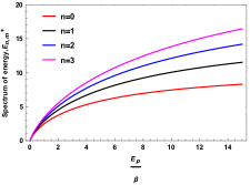
(a)

(b)

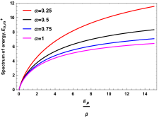
(c)

(d)

Figure 1: The energy spectrum $E_{n,m}^{+}$ for equation (16), where the parameters are set as $k=M=1,r=0.5.$

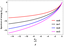
(a)

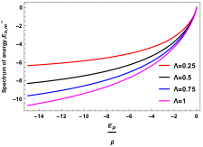
(b)

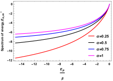
(c)

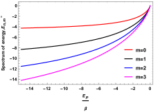
(d)

Figure 2: The energy spectrum $E_{m,n}^{-}$ for equation (16), where the parameters are set as $k=M=1,r=0.5.$

Now, we use two different types of rainbow function and obtain the expression of energy eigenvalue of he scalar bosons.

Case A: Rainbow functions $f(\chi)=\frac{(e^{\beta\,\chi}-1)}{\beta\,\chi}$, $h(\chi)=1$, and $\chi=\frac{|E|}{E_{p}}$

Here, we obtain the eigenvalue solution of the above discussed quantum system using the following pair of the rainbow function given by [14]

$$f(\chi)=\frac{(e^{\beta\,\chi}-1)}{\beta\,\chi},\quad h(\chi)=1.$$ (14)

Thereby, substituting this rainbow function into the relation (13), we obtain

$$\frac{E^{2}_{p}\,\Big{(}e^{\frac{\beta\,E}{E_{p}}}-1\Big{)}^{2}}{\beta^{2}}=M^{2}+k^{2}+\Lambda\,\Big{(}2\,n+\frac{3}{2}+\frac{|m|}{|\alpha|}\Big{)}^{2}\,\frac{\pi^{2}}{2\,r^{2}_{0}}.$$ (15)

Simplification of the above relation results the following expression of the energy eigenvalue given by

$$E^{\pm}_{n,m}=\frac{E_{p}}{\beta}\,\mbox{ln}\Bigg{[}1\pm\frac{1}{(E_{p}/\beta)}\sqrt{M^{2}+k^{2}+\Lambda\,\Big{(}2\,n+\frac{3}{2}+\frac{|m|}{|\alpha|}\Big{)}^{2}\,\frac{\pi^{2}}{2\,r^{2}_{0}}}\Bigg{]}.$$ (16)

Equation (16) is the relativistic energy profile of charge-free scalar bosons in BML space-time in the presence of rainbow gravity’s defined by the pair of rainbow function (14). We see that the relativistic energy spectrum is influenced by the topology of the geometry characterized by the parameter $\alpha$ and the cosmological constant $\Lambda$. Furthermore, the rainbow parameter $\beta<1$ also modified the energy profiles and shifted the results.

Case B: Rainbow functions $f(\chi)=1$, $h(\chi)=1+\beta\,\frac{\chi}{2}$, and $\chi=\frac{|E|}{E_{p}}$

In this case, we obtain the eigenvalue solution of the above discussed quantum system using the following pair of the rainbow function given by [42]

$$f(\chi)=1,\quad h(\chi)=1+\beta\,\frac{\chi}{2}.$$ (17)

Thereby, substituting this rainbow function into the relation (13), we obtain

$$E^{2}-M^{2}=\Delta\,\Big{(}1+\frac{\beta}{2\,E_{p}}\,E\Big{)}^{2},$$ (18)

where we have set

$$\Delta=k^{2}+\Lambda\,\Big{(}2\,n+\frac{3}{2}+\frac{|m|}{|\alpha|}\Big{)}^{2}\,\frac{\pi^{2}}{2\,r^{2}_{0}}.$$ (19)

Simplification of the above relation (18) results the following energy expression given by

$$E^{\pm}_{n,m}=\frac{1}{\Big{(}1-\frac{\Delta\,\beta^{2}}{4\,E^{2}_{p}}\Big{)}}\,\Bigg{[}\frac{\Delta\,\beta}{2\,E_{p}}\pm\sqrt{M^{2}\,\Bigg{(}1-\frac{\Delta\,\beta^{2}}{4\,E^{2}_{p}}\Bigg{)}+\Delta}\Bigg{]}.$$ (20)

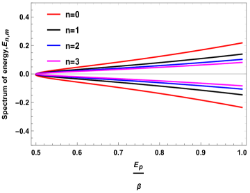
(a)

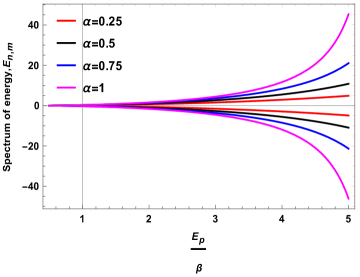
(b)

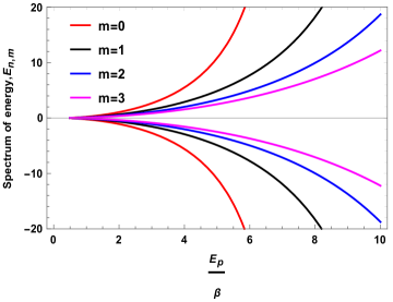
(c)

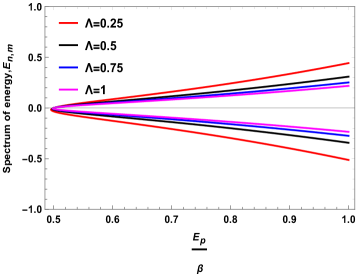
(d)

Figure 3: The energy spectrum $E^{\pm}_{m,n}$ for equation (20), where we set the parameters $k=M=1$, and $r=0.5.$

Equation (20) is the relativistic energy profile of charge-free scalar bosons in BML space-time in the presence of rainbow gravity’s defined by the pair of rainbow function (17). We see that the relativistic energy spectrum is influenced by the topology of the geometry characterized by the parameter $\alpha$ and the cosmological constant $\Lambda$. Furthermore, the rainbow parameter $\beta<1$ also modified the energy profiles and shifted the results.

We graphically depicted the energy spectrum $E^{\pm}_{n,m}$ of scalar particles as defined in Equation (16) in Figures 1–2 while varying different parameters, including the cosmological constant $\Lambda$, the topology parameter $\alpha$, the radial quantum number $n$, and the angular quantum number $m$. Our observations revealed that the energy level of scalar particles for a particular quantum state exhibit a parabolic nature. When we modify any one of the aforementioned parameters, this parabolic trend shifts upward with increased values. Similarly, we plotted the energy spectrum $E^{\pm}_{n,m}$ from Equation (20) in Figure 3 by choosing different values of the aforementioned parameters.

3 Quantum Oscillator Fields: The Klein-Gordon Oscillator

In this section, we study quantum oscillator field via the Klein-Gordon oscillator in the background of BML space-time under the influence of rainbow gravity’s. This oscillator field is studied by replacing the momentum operator into the Klein-Gordon equation via $\partial_{\mu}\to(\partial_{\mu}+M\,\omega\,X_{\mu})$, where the four-vector $X_{\mu}=(0,r,0,0)$ and $\omega$ is the oscillator frequency. The relativistic quantum oscillator fields in curved space-times background have been investigated by numerous authors (see, [50, 51, 52, 53, 54, 55, 56, 57, 58]).

Therefore, the relativistic wave equation describing the quantum oscillator fields is given by

$$\Big{[}\frac{1}{\sqrt{-g}}\,(\partial_{\mu}+M\,\omega\,X_{\mu})\,(\sqrt{-g}\,g^{\mu\nu})\,(\partial_{\nu}-M\,\omega\,X_{\nu})\Big{]}\,\Psi=M^{2}\,\Psi,$$ (21)

where $M$ is the rest mass of the particles, $\omega$ is the oscillator frequency, $X_{\mu}=(0,r,0,0)$ is the four-vector.

Expressing the wave equation (21) in the magnetic universe background (2), we obtain

$$\Bigg{[}-f^{2}\,\frac{d^{2}}{dt^{2}}+2\,\Lambda\,h^{2}\,\Bigg{\{}\frac{d^{2}}{dr^{2}}+\frac{1}{\tan r}\,\frac{d}{dr}-M\,\omega-\frac{M\,\omega\,r}{\tan r}-M^{2}\,\omega^{2}\,r^{2}+\frac{1}{\alpha^{2}\,\sin^{2}r}\,\frac{d^{2}}{d\phi^{2}}\Bigg{\}}$$

$$+h^{2}\,\frac{d^{2}}{dz^{2}}-M^{2}\Bigg{]}\,\Psi=0\,.$$ (22)

Substituting the wave function ansatz (7) into the above differential equation (22) results the following second-order differential equation form:

$$\psi^{\prime\prime}+\frac{1}{\tan r}\,\psi^{\prime}+\Bigg{[}\frac{(f^{2}\,E^{2}-M^{2})}{2\,\Lambda\,h^{2}}-M\,\omega-\frac{M\,\omega\,r}{\tan r}-M^{2}\,\omega^{2}\,r^{2}-\frac{k^{2}}{2\,\Lambda}-\frac{\iota^{2}}{\sin^{2}r}\Bigg{]}\,\psi=0,$$ (23)

We solve the above equation taking an approximation of the trigonometric function up to the first order, that is, $\sin r\approx r$, $\tan r\approx r$. Therefore, the radial wave equation (23) reduces to the following form:

$$\psi^{\prime\prime}+\frac{1}{r}\,\psi^{\prime}+\Bigg{[}\eta-M^{2}\,\omega^{2}\,r^{2}-\frac{\iota^{2}}{r^{2}}\Bigg{]}\,\psi=0,$$ (24)

where we have defined

$$\eta=\frac{(f^{2}\,E^{2}-M^{2})}{2\,\Lambda\,h^{2}}-\frac{k^{2}}{2\,\Lambda}-2\,M\,\omega.$$ (25)

We change the dependent variable via transformation $\psi(r)=\frac{1}{\sqrt{r}}\,R(r)$, equation (24) can be written as the compact Liouville’s normal form

$$\Bigg{(}\frac{d^{2}}{dr^{2}}-\sum^{2}_{i=-2}\,C_{i}\,r^{i}\Bigg{)}\,R(r)=0,$$ (26)

where we have set different coefficients

$$C_{-2}=\iota^{2}-\frac{1}{4},\quad C_{-1}=0,\quad C_{0}=-\eta,\quad C_{1}=0,\quad C_{2}=M^{2}\,\omega^{2}\,.$$ (27)

To solve the differential equation (26), one can write the second term of this equation, as summation of three terms, namely: linear plus oscillator term, Coulomb plus constant term and quadratic inverse term as follows [59]:

$$\sum^{2}_{i=-2}\,C_{i}\,r^{i}=V_{0}+V_{c}+V_{\infty},$$ (28)

where

$$V_{0}=\frac{C_{-2}}{r^{2}},\quad V_{c}=C_{0},\quad V_{\infty}=C_{2}\,r^{2}.$$ (29)

By using equation (28), we can expressed the function $R(r)$ as $R(r)=A_{0}(r)\,A(r)\,A_{\infty}(r)$, where $A(r)$ is an unknown function, and the functions $A_{0}(r)$, $A_{\infty}(r)$ are the asymptotic factors deduced from the potential functions $V_{0}(r)$ and $V_{\infty}(r)$, respectively. We obtain the asymptotic factors as follows:

$$A_{0}(r)=r^{\frac{1}{2}\Big{(}1+\sqrt{1+4\,C_{-2}}\Big{)}}=r^{\iota+1/2},$$

$$A_{\infty}(r)=e^{-\frac{1}{2}\,\sqrt{C_{2}}\,\Big{(}r+\frac{C_{1}}{2\,C_{2}}\Big{)}\,r}=e^{-\frac{1}{2}\,M\,\omega\,r^{2}}.$$ (30)

Therefore, one can write the radial wave function

$$R(r)=r^{\iota+1/2}\,e^{-\frac{1}{2}\,M\,\omega\,r^{2}}\,A(r).$$ (31)

Substituting this radial function $R(r)$ into the differential equation (26), we obtain the following differential equation form:

$$\Bigg{(}\frac{d^{2}}{dr^{2}}+\mathcal{P}(r)+\mathcal{Q}(r)\Bigg{)}\,A(r)=0.$$ (32)

Here we have defined

$$\mathcal{P}(r)=\sum^{1}_{i=-1}\,p_{i}\,r^{i},\quad\mathcal{Q}(r)=\sum^{0}_{i=-1}\,q_{i}\,r^{i},$$ (33)

where the coefficients $p_{-1},p_{0},p_{1},q_{-1},q_{0}$ are independent of the radial coordinate $r$ and are dependent only to the potential parameters $C_{i}$, where $(-2\leq i\leq 2)$ as follows:

$$p_{-1}=1+\sqrt{1+4\,C_{-2}}=1+2\,\iota\,$$

$$p_{0}=-\frac{C_{1}}{\sqrt{C_{2}}}=0,$$

$$p_{1}=-4\,\sqrt{C_{2}}=-4\,M\,\omega\,$$

$$q_{-1}=-\frac{C_{1}}{2\,\sqrt{C_{2}}}\,(1+\sqrt{1+4\,C_{-2}})=0,$$

$$q_{0}=-\sqrt{C_{2}}\,(2+\sqrt{1+4\,C_{-2}})=-2\,M\,\omega\,(1+\iota)\,.$$ (34)

To proceed further, we express the unknown function $A(r)$ in terms of power series around the origin given by [45]

$$A(r)=\sum^{\infty}_{i=0}\,d_{i}\,r^{i},$$ (35)

where the coefficients $d_{0},d_{1},d_{2},.....$ depend on the parameter $C_{i}$.

By substituting this power series (35) into the equation (32), one will find a three-term recurrence relation discussed given in Refs. [60, 61]. This power series function (35) becomes a finite degree polynomial by imposing the following condition (see Refs. [60, 61] for the energy quantization condition) given by

$$n\,p_{1}-C_{0}+q_{0}=0\quad(n=0,1,2,3,...).$$ (36)

Simplification of the above condition gives us the following energy relation given by

$$f^{2}\,E^{2}=M^{2}+h^{2}\,\Bigg{[}k^{2}+8\,M\,\omega\,\Lambda\,\Big{(}n+1+\frac{\iota}{2}\Big{)}\Bigg{]}\,.$$ (37)

Here also, we use two pair of rainbow function stated in the previous section and obtain the energy eigenvalue expression of the oscillator fields.

Case A: Rainbow functions $f(\chi)=\frac{(e^{\beta\,\chi}-1)}{\beta\,\chi}$, $h(\chi)=1$, and $\chi=\frac{|E|}{E_{p}}$

Substituting this pair of the rainbow function $f(\chi)=\frac{(e^{\beta\,\chi}-1)}{\beta\,\chi}$, $h(\chi)=1$ [14] into the relation (37), we obtain the following quadratic equation for $E$ given by

$$\frac{E^{2}_{p}\,\Big{(}e^{\frac{\beta\,E}{E_{p}}}-1\Big{)}^{2}}{\beta^{2}}=M^{2}+k^{2}+8\,M\,\omega\,\Lambda\,\Big{(}n+1+\frac{|m|}{2\,|\alpha|}\Big{)}\,.$$ (38)

Simplification of the above equation results the following energy expression associated with the mode $\{n,m\}$ given by

$$E^{\pm}_{n,m}=\frac{E_{p}}{\beta}\,\mbox{ln}\,\Bigg{[}1\pm\frac{1}{(E_{p}/\beta)}\sqrt{M^{2}+k^{2}+8\,M\,\omega\,\Lambda\,\Big{(}n+1+\frac{|m|}{2\,|\alpha|}\Big{)}}\Bigg{]}\,.$$ (39)

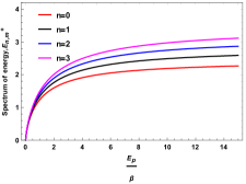
(a)

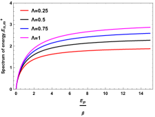
(b)

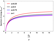
(c)

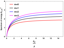
(d)

Figure 4: The energy spectrum $E_{m,n}^{+}$ for the relation given in equation (39), where the parameters are set as $k=M=1$ and $\omega=0.5$.

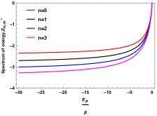
(a)

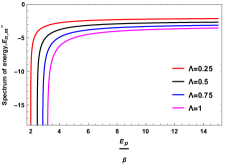
(b)

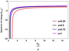
(c)

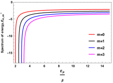
(d)

Figure 5: The energy spectrum $E_{m,n}^{-}$ for the relation given in equation (39), where the parameters are set as $k=M=1$ and $\omega=0.5$.

Equation (39) is the relativistic energy profile of oscillator fields in BML space-time in the presence of rainbow gravity’s defined by the pair of rainbow function (14). We see that the energy spectrum is influenced by the topology of the geometry characterized by the parameter $\alpha$, the cosmological constant $\Lambda$, and changes with change in the oscillator frequency $\omega$. Furthermore, the rainbow parameter $\beta<1$ also modified the energy profiles and shifted the results.

Case B: Rainbow functions $f(\chi)=1$, $h(\chi)=1+\beta\,\frac{\chi}{2}$, and $\chi=\frac{|E|}{E_{p}}$

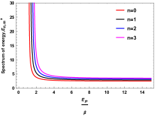
(a)

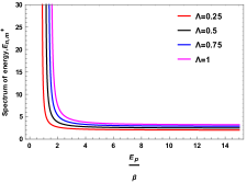
(b)

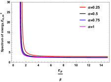
(c)

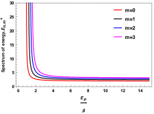
(d)

Figure 6: The energy spectrum $E_{m,n}^{+}$ for the relation given in equation (42), where the parameters are set as $k=M=1$ and $\omega=0.5$.

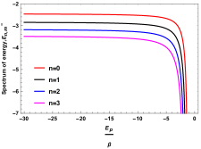
(a)

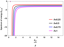
(b)

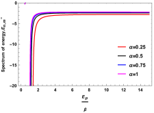
(c)

(d)

Figure 7: The energy spectrum $E_{m,n}^{-}$ for the relation given in equation (42), where the parameters are set as $k=M=1$ and $\omega=0.5$.

Substituting this pair of the rainbow function $f(\chi)=1$, $h(\chi)=1+\beta\,\frac{\chi}{2}$ [42] into the relation (37), we obtain the following quadratic equation for $E$ given by

$$E^{2}-M^{2}=\Theta\,\Big{(}1+\frac{\beta}{2\,E_{p}}\,E\Big{)}^{2},$$ (40)

where we set

$$\Theta=k^{2}+8\,M\,\omega\,\Lambda\,\Big{(}n+1+\frac{|m|}{2\,|\alpha|}\Big{)}\,.$$ (41)

Simplification of the above equation (40) results the following energy expression associated with the mode $\{n,m\}$ given by

$$E^{\pm}_{n,m}=\frac{1}{\Bigg{[}1-\frac{\Theta}{4}\,\Big{(}\frac{\beta}{E_{p}}\Big{)}^{2}\Bigg{]}}\,\Bigg{[}\frac{\Theta}{2}\,\frac{\beta}{E_{p}}\pm\sqrt{M^{2}\,\Bigg{[}1-\frac{\Theta}{4}\,\Big{(}\frac{\beta}{E_{p}}\Big{)}^{2}\Bigg{]}+\Theta}\Bigg{]}.$$ (42)

Equation (42) is the relativistic energy profile of oscillator fields in BML space-time in the presence of rainbow gravity’s defined by the pair of rainbow function (17). We see that energy spectrum is influenced by the topology of the geometry characterized by the parameter $\alpha$, the cosmological constant $\Lambda$, and the oscillator frequency $\omega$. Furthermore, the rainbow parameter $\beta<1$ also modified the energy profiles and shifted the results.

We graphically depicted the energy spectrum $E^{\pm}_{n,m}$ of oscillator fields as defined in Equation (39) in Figures 4-5 while varying different parameters, including the cosmological constant $\Lambda$, the topology parameter $\alpha$, the radial quantum number $n$, and the angular quantum number $m$. Our observations revealed that the energy levels for a particular quantum state exhibit a parabolic nature. When we modify any one of the aforementioned parameters, this parabolic trend shifts upward with increased values. Similarly, we plotted the energy spectrum $E^{\pm}_{n,m}$ from Equation (42) in Figures 6-7 and noted a decreasing trend in the energy levels. This pattern shifts upward with increasing values of any of the aforementioned parameters.

4 Conclusions

The relativistic quantum dynamics of various particles, such as spin-0 charge-free and charged scalar particles, spin-1/2 fermionic fields, and relativistic spin-1 fields in a curved space-time background, yields profound results compared to those obtained in flat space or within Landau levels. Numerous authors have introduced external magnetic and scalar potentials (including linear confining, Coulomb-type, Cornell-type, Yukawa potential, Kratzer potential etc.) into these quantum systems, leading to intriguing findings. Furthermore, the presence of topological defects caused by cosmic strings, global monopoles, and spinning cosmic strings induces shifts in the energy spectrum of these particles in the quantum realm. Various curved spaces have been considered in the context of quantum systems, such as Gödel and Gödel-type space-times, Kerr-Newman solutions, and others. Researchers have obtained the relativistic energy profiles of these particles in these curved space-time backgrounds, shedding light on the rich and complex behavior of quantum systems in diverse geometric and topological scenarios.

Rainbow gravity is an intriguing phenomenon in physics that leads to modifications in the relativistic mass-energy relation within the framework of special relativity theory. Consequently, the exploration of rainbow gravity’s implications in quantum mechanical problems has become a focal point of research interest. Various studies have delved into the effects of rainbow gravity in different quantum systems, including the Dirac oscillator in cosmic string space-time [41], the dynamics of scalar fields in a wormhole background with cosmic strings [62], quantum motions of scalar particles [63], and the behavior of spin-1/2 particles in a topologically trivial Gödel-type space-time [64]. Additionally, investigations have extended to the motions of photons in cosmic string space-time [65] and the generalized Duffin–Kemmer–Petiau equation with non-minimal coupling in cosmic string space-time [66]. In the present study, we explored another four-dimensional geometry known as Bonnor-Melvin-Lambda space-time, examining the quantum motions of scalar and oscillator fields under the influence of rainbow gravity.

In Section 2, we derive the radial equation of the Klein-Gordon equation, which describes the dynamics of charge-free spin-0 scalar particles in the Bonnor-Melvin-Lambda (BML) space-time under the influence of rainbow gravity. Subsequently, we solve this radial equation by selecting two pairs of rainbow functions, resulting in the approximate energy eigenvalues for scalar particles given by Equations (16) and (20). Moving on to Section 3, we explored quantum oscillator fields using the Klein-Gordon oscillator in the BML space-time under the effects of rainbow gravity. Employing the same pairs of rainbow functions, we obtain approximate energy profiles, as outlined in Equations (39) and (42). Throughout both studies, we demonstrate that the energy profiles of scalar and oscillator fields are influenced by the topology parameter $\alpha$ and the cosmological constant $\Lambda$. Additionally, in the context of quantum oscillator fields, the frequency of oscillation $\omega$ also modifies the energy spectrum. Another noteworthy aspect is that the energy spectrum for both scalar and oscillator fields depends on the quantum numbers $\{n,m\}$ and, consequently, undergoes changes in their values. We visually represented these energy spectra for scalar and oscillator fields across various values of the aforementioned parameters in Figures 1–7.

Our findings highlight the intricate interplay between the dynamics of quantum particles and the strength of the magnetic field in the BML space-time, providing valuable insights into the behavior of scalar and oscillator fields under the influence of rainbow gravity.

Conflict of Interest

There is no conflict of interests in this paper.

Funding Statement

No fund has received for this paper.

Data Availability Statement

No data were generated or analysed during this study.

References

- [1] A. Einstein, Annalen Phys. 49, 769 (1916) https://doi.org/10.1002/20andp.200590044. .
- [2] B. P. Abbott et al, Phys Rev Lett 116, 061102 (2016) https://doi.org/10.1103/PhysRevLett.116.061102.
- [3] K. Akiyama et al, Astrophys J Lett 875, L1 (2019) https://doi.org/10.3847/2041-8213/ab0f43.
- [4] R. P. Feynman, and A. R. Hibbs, Quantum mechanics and path integrals, Dover Publications Inc. (1965).
- [5] G. Amelino-Camelia, Phys. Lett. B 510, 255 (2001) https://doi.org/10.1016/S0370-2693(01)00506-8..
- [6] G. Amelino-Camelia, Int. J. Mod. Phys D 11, 35 (2002) https://doi.org/10.1142/S0218271802001330..
- [7] G. Amelino-Camelia, J. Kowalski-Glik, G. Mandanici, A. Procaccini, Int. J. Mod. Phys. A 20, 6007 (2005) https://doi.org/10.1142/S0217751X05028569.
- [8] J. Magueijo, L. Smolin, Phys. Rev. Lett. 88, 190403 (2002) https://doi.org/10.1103/PhysRevLett.88.190403.
- [9] J. Magueijo, L. Smolin, Phys. Rev. D 67, 044017 (2003) https://doi.org/10.1103/PhysRevD.67.044017.
- [10] L. Smolin, Nucl. Phys. B 742, 142 (2006) https://doi.org/10.1016/j.nuclphysb.2006.02.017.
- [11] S. Ghosh, Phys. Rev. D 74, 084019 (2006) https://doi.org/10.1103/PhysRevD.74.084019.
- [12] Y. Ling, Q. Wu, Phys. Lett. B 687, 103 (2010) https://doi.org/10.1016/j.physletb.2010.03.028.
- [13] A. Ashour, M. Faizal, A. F. Ali, F. Hammad, Eur. Phys. J. C 76, 264 (2016) https://doi.org/10.1140/epjc/s10052-016-4124-7.
- [14] G. Amelino-Camelia, J. R. Ellis, N. E. Mavromatos, D. V. Nanopoulos, S. Sarkar, Nature 393, 763 (1998) https://doi.org/10.1038/31647.
- [15] G. Amelino-Camelia, J. R. Ellis, N. E. Mavromatos, D. V. Nanopoulos, Int. J. Mod. Phys. A 12, 607 (1997) https://doi.org/10.1142/S0217751X97000566.
- [16] V. A. Kostelecký, S. Samuel, Phys. Rev. D 39, 683 (1989) https://doi.org/10.1103/PhysRevD.39.683.
- [17] R. Gambini, J. Pullin, Phys. Rev. D 59, 124021 (1999) https://doi.org/10.1103/PhysRevD.59.124021.
- [18] G. T. Hooft, Class. Quantum Grav. 13, 1023 (1996) https://doi.org/10.1088/0264-9381/13/5/018.
- [19] S. M. Carroll, J. A. Harvey, V. A. Kostelecký, C. D. Lane, T. Okamoto, Phys. Rev. Lett. 87, 141601 (2001) https://doi.org/10.1103/PhysRevLett.87.141601.
- [20] B. Majumder, Int. J. Mod. Phys. D 22, 1350079 (2013) https://doi.org/10.1142/S021827181350079X.
- [21] S. H. Hendi, M. Momennia, B. Eslam-Panah, S. Panahiyan, Phys. Dark Univ. 16, 26 (2017) https://doi.org/10.1016/j.dark.2017.04.001.
- [22] S. H. Hendi, M. Faizal, B. Eslam-Panah, S. Panahiyan, Eur. Phys. J. C 76, 296 (2016) https://doi.org/10.1140/epjc/s10052-016-4119-4.
- [23] C. Leiva, J. Saavedra, J. Villanueva, Mod. Phys. Lett. A 24, 1443 (2009) https://doi.org/10.1142/S0217732309029983.
- [24] H. Li, Y. Ling, X. Han, Class. Quantum Grav. 26, 065004 (2009) https://doi.org/10.1088/0264-9381/26/6/065004.
- [25] V. B. Bezerra, H .F. Mota, C. R. Muniz, EPL 120, 10005 (2017) https://doi.org/10.1209/0295-5075/120/10005.
- [26] J. Magueijo, L. Smolin, Class. Quantum Grav. 21, 1725 (2004), https://doi.org/10.1088/0264-9381/21/7/001.
- [27] G. Amelino-Camelia, Symmetry 2010, 2 (1), 230 https://doi.org/10.3390/sym2010230.
- [28] A. A. Abdo et al., Nature 462, 331 (2009) https://doi.org/10.1038/nature08574.
- [29] S. Zhang, B. Q. Ma, Astropart. Phys. 61, 108 (2014) https://doi.org/10.1016/j.astropartphys.2014.04.008.
- [30] G. Amelino-Camelia, G. D’Amico, G. Rosati, and N. Loret, Nat. Astron. 1, 0139 (2017) https://doi.org/10.1038/s41550-017-0139.
- [31] W. B. Bonner, Proc. Phys. Soc. A 67, 225 (1954) https://doi.org/10.1088/0370-1298/67/3/305.
- [32] M. A. Melvin, Phys. Lett. 8 (1965) 65 https://doi.org/10.1016/0031-9163(64)90801-7.
- [33] M. Astorino, JHEP 06 (2012) 086 https://doi.org/10.1007/JHEP06(2012)086.
- [34] J. Vesely and M. Z̆ofka, Phys. Rev. D 100, 044059 (2019) https://doi.org/10.1103/PhysRevD.100.044059.
- [35] M. Žofka, Phys. Rev. D 99, 044058 (2019) https://doi.org/10.1103/PhysRevD.99.044058.
- [36] E. R. Figueiredo Medeiros and E. R. Bezerra de Mello, Eur. Phys. J. C 72, 2051 (2012) https://doi.org/10.1140/epjc/s10052-012-2051-9.
- [37] L. B. Castro, Eur. Phys. J. C 75, 287 (2015) https://doi.org/10.1140/epjc/s10052-015-3507-5.
- [38] H. Hassanabadi, A. Afshardoost and S. Zarrinkamar, Ann. Phys. (N. Y.) 356, 346 (2015) https://doi.org/10.1016/j.aop.2015.02.027.
- [39] R. L. L. Vitoria and K. Bakke, Eur. Phys. J. C 78, 175 (2018) https://doi.org/10.1140/epjc/s10052-018-5658-7.
- [40] H. F. Mota and K. Bakke, Phys. Rev. D 89, 027702 (2014) https://doi.org/10.1103/PhysRevD.89.027702.
- [41] K. Bakke, H. Mota, Eur. Phys. J. Plus 133, 409 (2018) https://doi.org/10.1140/epjp/i2018-12268-6.
- [42] A. F. Grillo and E. Luzio and F. Méndez, Phys. Rev. D 77, 104033 (2008) https://doi.org/10.1103/PhysRevD.77.104033.
- [43] W. Greiner, Relativistic Quantum Mechanics. Wave Equations, Springer-Verlag, Berlin, Gemnay (2000).
- [44] M. Abramowitz and I. A. Stegun, Handbook of Mathematical Functions with Formulas, Graphs, and Mathematical Tables, New York: Dover (1972).
- [45] G. B. Arfken, H. J. Weber and F. E. Harris, Mathematical Methods for Physicists, Elsevier (2012).
- [46] R. L. L. Vitoria, K. Bakke, Int. J. Mod. Phys. D 27, 1850005 (2018) https://doi.org/10.1142/S0218271818500050.
- [47] K. Bakke, Eur. Phys. J. B 85, 354 (2012) https://doi.org/10.1140/epjb/e2012-30490-6.
- [48] A. V. D. M. Maia, K. Bakke, Physica B 531, 213 (2018) https://doi.org/10.1016/j.physb.2017.12.045.
- [49] E. A. F. Bragança, R. L. L. Vitória, H. Belich, E. R. Bezerra de Mello, Eur. Phys. J. C 80, 206 (2020) https://doi.org/10.1140/epjc/s10052-020-7774-4.
- [50] F. Ahmed, Int. J. Mod. Phys. A 37, 2250186 (2022) https://doi.org/10.1142/S0217751X2250186X.
- [51] F. Ahmed, Commun. Theor. Phys. 75, 025202 (2023) https://doi.org/10.1088/1572-9494/aca650.
- [52] L. C. N. Santos, C. E. Mota, and C. C. Barros Jr., Adv. High Energy Phys. 2019, 2729352(2019) https://doi.org/10.1155/2019/2729352.
- [53] Y. Yang, Z.-W. Long, Q.-K. Ran, H. Chen, Z.-L. Zhao, and C.-Y. Long, Int. J. Mod. Phys. A 36, 2150023 (2021) https://doi.org/10.1142/S0217751X21500238.
- [54] A. R. Soares, R. L. L. Vitória, and H. Aounallah, Eur. Phys. J. Plus 136, 966 (2021) https://doi.org/10.1140/epjp/s13360-021-01965-0.
- [55] A. Bouzenada, A. Boumali, Ann. Phys. 452, 169302 (2023) https://doi.org/10.1016/j.aop.2023.169302.
- [56] A. Bouzenada, A. Boumali, R. L. L. Vitoria, F. Ahmed and M. Al-Raeei, Nucl. Phys. B 994, 116288 (2023) https://doi.org/10.1016/j.nuclphysb.2023.116288.
- [57] A. Bouzenada, A. Boumali and F. Serdouk, Theor. Math. Phys,216, 1055–1067 (2023) https://doi.org/10.1134/S0040577923070115.
- [58] A. Bouzenada, A. Boumali, and E. O. Silva, Ann. Phys. 458,169479 (2023) https://doi.org/10.1016/j.aop.2023.169479.
- [59] J. Karwowski and H. A. Witek, Theor. Chem. Acc. 133, 1494 (2014) https://doi.org/10.1007/s00214-014-1494-5.
- [60] M. Eshghi, H. Mehraban and I. A. Azar, Physica E: Low-dimensional Syst. Nanostruc. 94, 106 (2017) https://doi.org/10.1016/j.physe.2017.07.024.
- [61] M. Eshghi, H. Mehraban and I. A. Azar, Eur. Phys. J. Plus 132, 477 (2017) https://doi.org/10.1140/epjp/i2017-11728-9.
- [62] F. Ahmed and A. Guvendi, Chinese Journal of Physics (2023), https://doi.org/10.1016/j.cjph.2023.11.028.
- [63] E. E. Kangal, M. Salti, O. Aydogdu and K. Sogut, Phys. Scr. 96 (2021) 095301 https://doi.org/10.1088/1402-4896/ac02f1.
- [64] E. E. Kangal, K. Sogut, M. Salti and O. Aydogdu. Ann. Phys. 444 (2022) 169018 https://doi.org/10.1016/j.aop.2022.169018.
- [65] K. Sogut, M. Salti and O. Aydogdu, Ann. Phys. 431 (2021) 168556 https://doi.org/10.1016/j.aop.2021.168556.
- [66] M. Hosseinpour, H. Hassanabadi, J. Kriz, S. Hassanabadi and B. C. Lütfüoğlu, Int. J Geom. Meths. Mod. Phys. 18, 2150224 (2021) https://doi.org/10.1142/S0219887821502248.