Adaptive Proximal Policy Optimization with Upper Confidence Bound

Ziqi Zhang    Jingzehua Xu    Zifeng Zhuang    Jinxin Liu    Donglin wang
Abstract

Trust Region Policy Optimization (TRPO) attractively optimizes the policy while constraining the update of the new policy within a trust region, ensuring the stability and monotonic optimization. Building on the theoretical guarantees of trust region optimization, Proximal Policy Optimization (PPO) successfully enhances the algorithm’s sample efficiency and reduces deployment complexity by confining the update of the new and old policies within a surrogate trust region. However, this approach is limited by the fixed setting of surrogate trust region and is not sufficiently adaptive, because there is no theoretical proof that the optimal clipping bound remains consistent throughout the entire training process, truncating the ratio of the new and old policies within surrogate trust region can ensure that the algorithm achieves its best performance, therefore, exploring and researching a dynamic clip bound for improving PPO’s performance can be quite beneficial. To design an adaptive clipped trust region and explore the dynamic clip bound’s impact on the performance of PPO, we introduce an adaptive PPO-CLIP (Adaptive-PPO) method that dynamically explores and exploits the clip bound using a bandit during the online training process. Furthermore, ample experiments will initially demonstrate that our Adaptive-PPO exhibits sample efficiency and performance compared to PPO-CLIP.

Machine Learning, ICML

1 Introduction

Typically, there are primarily two common paradigms in reinforcement learning (RL). The first involves alternating between learning Q-networks and using them to update the policy network (Mnih et al., 2013, 2015). The second paradigm, based on gradient methods (Lillicrap et al., 2019), directly updates the policy. The second paradigm is applicable in environments with high-dimensional action spaces and exhibits higher sample efficiency. But, gradient-based paradigms are generally on-policy methods, meaning that the current policy may not fully utilize the collected dataset.

To fully utilize the collected dataset and train the current policy using policy gradient-based methods, we can introduce importance sampling, effectively approximating on-policy algorithms to off-policy ones. However, when updating the policy, we often encounter the issue of step size, where the new policy update may deviate too far from the old policy, making it difficult for the policy to reach the optimal solution. TRPO (Schulman et al., 2017a) proposes, by introducing importance sampling and using the Kullback-Leibler (KL) divergence to constrain the distance between the old policy and the new policy, to ensure policy improvement while preventing the new policy from deviating too far due to overly large step sizes and failing to reach the optimal value.

Although TRPO has mathematically proven its ability to guarantee monotonic policy improvement, fitting TRPO’s objective, especially the KL divergence between old and new policies, requires a significant amount of computational resources, which is impractical in scenarios with lower interaction costs. To further enhance TRPO and increase its practicality, PPO (Schulman et al., 2017b) introduces a similar clipped surrogate objective, which is also a KL divergence term, but limits the policy update within a fixed $\epsilon$ trust region. With this similar objective function, PPO achieves higher sample efficiency and computing efficiency, and increasing its real-world applicability.

Given that PPO can ensure monotonic policy improvement, is relatively easy to deploy, and exhibits a high degree of sample efficiency, PPO has been widely applied in various online RL scenarios (Nahrendra et al., 2023; Yang et al., 2022). Moreover, a range of research efforts have been made to modify PPO to further enhance its sample efficiency and performance (Schulman et al., 2018) or be scaled to more scenarios (Yu et al., 2022; Zhuang et al., 2023; Yu et al., 2022). Different from these improvements, our research primarily focuses on dynamically controlling the distance between the new and old policies, which is the updating step size, to further enhance the performance of PPO. Before introducing our method, we first examine the potential impact of updating step sizes on PPO performance from multiple perspectives: Policies at different stages require different sizes of clipping bounds. For example, when training starts, a larger clipping bound is needed to allow the new policy to deviate significantly from the old policy, thereby increasing sample efficiency. As the policy gradually converges, a smaller clipping bound is needed to maintain the stability of the policy. Given that controlling the step size of policy updates is crucial. Next, we will elucidate how to dynamically adjust the clip bound to control the magnitude of policy updates.

In order to dynamically adjust the clip bound of PPO during online training, we propose a bandit-based approach to dynamically balance the exploration and exploitation of a set of candidate clip bounds. Specifically, we maximize the upper confidence bound (UCB) value for each candidate bound to guide PPO in using different clip bounds during different stages of online training. Compared to using a fixed trust region, our approach offers several advantages: 1) By updating multiple clip bounds’ UCB based on the agent’s training performance in each episode, we can guide the selection of better clip bounds in each online training stage. 2) Our method can be used as a plug-and-play solution for any algorithm that requires dynamic control over update step sizes to better constrain their trust region. Compare to traditional adaptive surrogate trust region optimization (Chen et al., 2018), our approach has advantage that it can dynamically adjust the surrogate trust region via bandit-based approach thus don’t requiring excessive computational resource consumption, and our method responds to the requirements of the training task that is the selection of the clipping bound matches the maximization of the task’s return. To summarize, our contributions can be summarized as follows:

  • We analyze and provide the necessity of dynamically changing of PPO’s clipping boundaries, and proposing our method Adaptive-PPO which can dynamically change the PPO’s clipping boundaries across whole training phages thereby enabling the stable and monotonic policy improvement.

  • We provide the theoretical upper bound of PPO-CLIP and Adaptive-PPO by optimizing lag-Lagrange dual issue.

2 Preliminary

2.1 Reinforcement Learning.

We formulate RL as Markov decision Process (MDP) Tuple i.e.$\mathcal{M}:=(\mathcal{A},\mathcal{S},\gamma,\mathcal{\tau}(\cdot|\mathbf{s},\mathbf{a}),p_{0})$. Specifically, $\mathcal{A}$ denotes action space, $\mathcal{S}$ denotes state space, $p_{0}$ denotes the initial state distribution, $\pi\rightarrow\mathcal{S}\times\mathcal{A}$ denotes the policy and $r:\mathcal{A}\times\mathcal{S}\rightarrow\mathbb{R}$ denotes the reward function, and $\gamma\in[0,1]$ denotes the discount factor. The goal of RL is to find the optimal policy to maximize the accumulated Return, i.e.$\pi:=\arg\max_{\pi}\mathbb{E}_{\tau\sim\pi(\tau)}[R(\tau)]$, where $\tau=\{\mathbf{s}_{0},\mathbf{a}_{0},\cdots,\mathbf{s}_{t},\mathbf{a}_{t}\}$ is the roll-out trajectory. Furthermore, we estimate the expected return of current state action by training Q network i.e.$Q(\mathbf{s},\mathbf{a})=\mathbb{E}_{(\mathbf{s},\mathbf{a})\sim\pi(\tau)}[R(\tau)|\mathbf{s}=\mathbf{s},\mathbf{a}=\mathbf{a}]$, and the expectation of $Q(\mathbf{s},\mathbf{a})$ by value network i.e.$V(\mathbf{s})=\mathbb{E}_{\mathbf{a}\sim\mathcal{A}}[Q(\mathbf{s},\mathbf{a})]$. Addtionally, based on whether they make full use of previous data to train current policy, RL can be divided into two paradigm: on-policy and off-policy. In the off-policy paradigm, the agent can fully utilize data collected at different time steps to train the current policy, resulting in higher sample efficiency. In contrast, the on-policy paradigm allows the agent to train the current policy only using data collected at the current time step. However, we can introduce importance sampling to effectively use historical replay buffer for training.

2.2 Trust Region Optimization

Importance Sampling

Algorithms like PPO and TRPO introduce importance sampling to approximate on-policy algorithms as off-policy algorithms. This enables the use of previously collected datasets for training the current policy using policy gradient method i.e.Equation 1.

$$\mathcal{J}_{\pi_{new}}=\max\mathbb{E}_{\tau\sim\pi_{old}}[\frac{\pi_{\rm new}}{\pi_{\rm old}}A^{\pi_{\rm old}}],$$ (1)

KL Divergence and Trust Region Optimization

directly optimize Equation 1 may lead to the new policy diverging from the old policy, making it challenging to reach the optimal solution. Therefore, it’s necessary to further minimize the KL divergence between the new and old policies, thus constraining the policy updates within a specific trust region i.e.Equation 2.

$$\begin{split}\mathcal{J}_{\pi_{old}}=\max\mathbb{E}_{\tau\sim\pi_{old}}[\frac{\pi_{\rm new}}{\pi_{\rm old}}A^{\pi_{\rm old}}]+D_{\rm KL}(\pi_{\rm new}||\pi_{\rm old}),\end{split}$$ (2)

furthermore, in the clipped version of PPO, the proposal is to constrain the updates between the new and old policies within a fixed trust region, as indicated by Equation 3.

$$\begin{split}\mathcal{J}_{\pi_{new}}=\max\mathbb{E}_{\tau\sim\pi_{old}}[\min(\frac{\pi_{\rm new}}{\pi_{\rm old}}A^{\pi_{old}},{\rm clip}(\frac{\pi_{\rm new}}{\pi_{\rm old}},\\ 1-\epsilon,1+\epsilon)A^{\pi_{old}})],\end{split}$$ (3)

One of the advantages of PPO and TRPO is that their objective functions can guarantee monotonic policy improvement. In the following discussion, we will explore the theoretical connection between policy improvement, policy gradients, and advantage functions.

2.3 Guarantee of Monotonic Policy Improvement

the goal of policy optimization is to realize maximization of accumulated Return i.e.$\mathbb{E}_{\tau\sim\pi_{\rm new}}[R(\tau)]\geq\mathbb{E}_{\tau^{\prime}\sim\pi_{\rm old}}[R(\tau^{\prime})]$. To illustrate the relationship between policy improvement and advantage function, we first formulate the policy before updating as $\pi_{\rm old}$ while formulating the policy after updating as $\pi_{\rm new}$, furthermore, we formulate the advantage of current policy $\pi$ as Equation 4.

$\displaystyle\mathbb{E}_{\tau\sim\pi_{old}}[A^{\pi_{old}}(\mathbf{s},\mathbf{a})]$ $\displaystyle=\mathbb{E}_{\tau\sim\pi_{old}}[Q^{\pi_{old}}(\mathbf{s},\mathbf{a})]$ (4)
$\displaystyle-\mathbb{E}_{\tau\sim\pi_{old}}[V^{\pi_{old}}(\mathbf{s})]$

According to the advantage of $\pi_{new}$ over $\pi_{old}$ across whole training steps, the relationship between $\pi_{new}$ and $\pi_{old}$ can be described as Equation 5.

$\displaystyle\mathbb{E}_{\tau\sim\pi_{\rm new}}[R(\tau)]$ $\displaystyle=\mathbb{E}_{\tau\sim\pi_{\rm old}}[R(\tau)]$ (5)
$\displaystyle+\mathbb{E}_{\tau\sim\pi_{old}}[\sum_{t=0}^{t=T}\gamma^{t}A^{\pi_{old}}(\mathbf{s},\mathbf{a})].$

proof can be referred to (Kakade & Langford, 2002), and we also provide our proof latter.

Furthermore, .etal define the visitation frequency as Equation 6,

$$\rho_{\pi}(\mathbf{s})=P(\mathbf{s}_{0}=\mathbf{s})+\gamma P(\mathbf{s}_{1}=\mathbf{s})+\cdots+\gamma^{t}P(\mathbf{s}_{t}=\mathbf{s}),$$ (6)

and rewrite Equation 5 to Equation 7, the mainly difference between Equation 5 and Equation 7 is that Equation 7 take state visitation into consideration.

$$\begin{split}\mathbb{E}_{\tau\sim\pi_{\rm new}}[R(\tau)]&\geq\mathbb{E}_{\tau\sim\pi_{\rm old}}[R(\tau)]\\ &+\sum_{s}\rho_{\pi_{old}}\sum_{\mathbf{a}}\pi_{old}(\mathbf{a}|\mathbf{s})A^{\pi_{old}}(\mathbf{s},\mathbf{a}),\end{split}$$ (7)

thereby, if we want to guarantee $\mathbb{E}_{\tau\sim\pi_{\rm new}}[R(\tau)]\geq\mathbb{E}_{\tau^{\prime}\sim\pi_{\rm old}}[R(\tau^{\prime})]$, we just have to guarantee $\sum_{s}\rho_{\pi_{old}}\sum_{\mathbf{a}}\pi_{old}(\mathbf{a}|\mathbf{s})A^{\pi_{new}}(\mathbf{s},\mathbf{a})\geq 0$. However, it’s hard to directly optimize Equation 7, we can instead optimizing Equation 8.

$\displaystyle\mathcal{J}_{\pi_{old}}(\pi_{new})$ $\displaystyle=\mathbb{E}_{\tau\sim\pi_{\rm old}}[R(\tau)]$ (8)
$\displaystyle+\sum_{s}\rho_{\pi_{new}}\sum_{\mathbf{a}}\pi_{new}(\mathbf{a}|\mathbf{s})A^{\pi_{old}}(\mathbf{s},\mathbf{a}),$

Furthermore, Kakade and Langford implies that if $\pi_{new}$ exhibits small improvement compared to $\pi_{old}$ i.e.conducing conservative policy iteration via Equation 9.

$$\pi_{new}=\alpha\cdot\pi_{old}+(1-\alpha)\cdot\pi_{new},$$ (9)

where $\pi_{new}=\arg\max_{\pi_{new}}L_{\pi_{new}}(\pi_{old})$, it can guarantee the increase of $\mathcal{J}_{\pi_{old}}(\pi_{new})$, while satisfying the lower bound in Equation 10.

$$\begin{split}\mathbb{E}_{\tau\sim\pi_{new}}\geq L_{\pi_{old}}(\pi_{new})-\frac{2\epsilon\gamma}{(1-\gamma)^{2}}\alpha^{2},\end{split}$$ (10)

where $\epsilon=\max_{\mathbf{s},\mathbf{a}}\|A(\mathbf{s},\mathbf{a})\|$, following by this derivation and further extend Equation 10 from mixture policy to stochastic policy with a distance to measure $\pi_{old}$ and $\pi_{new}$, thereby obtaining the objective of TRPO, i.e.Equation 11.

$$\begin{split}\mathcal{J}(\pi_{new})=\mathcal{J}_{\pi_{old}}(\pi_{new})-C\cdot D_{\rm KL}(\pi_{new}||\pi_{\rm old}),\\ s.t.\,\,\min D_{KL}(\pi_{new}||\pi_{old})\end{split}$$ (11)

where $C=\frac{2\epsilon\gamma}{(1-\gamma)^{2}}\alpha^{2},$ and $\alpha=D_{TV}^{max}(\pi_{new}||\pi_{old})$.

benefit from the monotonic policy improvement guarantee of TRPO, PPO (Schulman et al., 2017b) propose the clipped trust region optimization i.e.Equation 3, which increasing the sample efficiency while reducing the difficulty of deployment.

In the above discussion (Section Introduction), we already mentioned the limitations of using a fixed clip bound to constrain PPO. Therefore, we introduced adaptive PPO (Adaptive-PPO), which dynamically adjusts the clipping bound in different online stages to truncate the KL divergence between $\pi_{old}$ and $\pi_{new}$. This approach caters to the agent’s varying needs for exploration and conservative learning at different online training stages. Before formally introducing our method, we firstly provide an introduction to Bandit and Upper Confidence Bound (UCB).

Bandit and Upper Confidence Bound (UCB)

UCB is a classical strategy algorithm based on uncertainty using the Hoeffding’s inequality, which can be expressed as Equation 12:

$$P(E[X]\geq\bar{x}_{n}+u)\leq\exp{(-2nu^{2})},$$ (12)

where $X_{1},\cdots,X_{n}\in[0,1]$ are $n$ independent and equally distributed random variables, and the empirical expectation is $\bar{x}_{n}$, which is formulated as Equation 13:

$$\bar{x}_{n}=\frac{1}{n}\sum_{j=1}^{n}X_{j}.$$ (13)

Now apply Hoeffding’s inequality to the bandit problem, and $c_{i}$ denotes the $i_{th}$ bandit. Substituting $\hat{Q}^{UCB}(c_{i})$ into $\bar{x}_{t}$, and the parameter $u=\hat{U}(c_{i})$ in the inequality represents the measure of uncertainty. Given a probability $p$ as Equation 14:

$$p=\exp(-2N(c_{i})U(c_{o})^{2}).$$ (14)

According to Hoeffding’s inequality, the $i_{th}$ bandit satisfy such relationship: $Q^{UCB}(c_{i})<\hat{Q}^{UCB}(c_{i})+\hat{U}(c_{i})$ holds with at least probability $1-p$. When $p$ is very small, $Q^{UCB}(c_{i})<\hat{Q}^{UCB}(c_{i})+\hat{U}(c_{i})$ is established with large probability, where $\hat{Q}^{UCB}(c_{i})+\hat{U}(c_{i})$ is the upper bound of the expected reward. In this case, the UCB algorithm selects the action that is expected to reward the highest upper bound, i.e.Equation 15:

$$c=\arg\max_{c\in\mathcal{C}}[\hat{Q}^{UCB}(c)+\hat{U}(c)].$$ (15)

Meanwhile, $\hat{U}(c_{i})$ can be derived from the Equation 14, thus the formulation of $\hat{U}(c_{i})$ can be expressed as Equation 16:

$$\hat{U}(c_{t})=\sqrt{\frac{\log{p}}{2N(c_{t})}}.$$ (16)

Therefore, after setting a probability $p$, we can compute the corresponding uncertainty measure $\hat{U}(c_{t})$. More intuitively, the UCB algorithm first estimates the upper bound of the expected reward of pulling each bar before selecting each bar, so that the expected reward of pulling each pull bar has only a small probability $p$ exceeding this upper bound, and then selects the bar with the largest upper bound of the expected reward, so as to select the bar most likely to get the maximum expected return.

In the specific implementation process, probability $p$ is usually set as $\frac{1}{t}$, adding the constant 1 to the denominator for the number of times each tie rod is pulled, so as to avoid the occurrence of numerical explosion. Thus, the formulation of $\hat{U}(c_{t})$ can be written as Equation 17:

$$\hat{U}(c_{t})=\sqrt{\frac{\log{p}}{2(N(c_{t})+1)}}.$$ (17)

Meanwhile, we set up a coefficient $\lambda_{c}$ to control the proportion of uncertainty, which can be formulated as Equation 18:

$$c_{t}=\arg\max_{c\in\mathcal{A}}[\hat{Q}^{UCB}(c)+\lambda_{c}\hat{U}(c)],$$ (18)

3 Adaptive Clip PPO (Adaptive-PPO)

Problem Formation.

Before formally proposing our method, we first formulate the dynamical changing of clipping bound as a UCB problem setting, that is first initializing n bandit arm as n clipping bounds for PPO updating, following by sampling arm for any training iteration with consideration of UCB values of these clipping bounds. Specifically, we first initialize n bandit arms i.e.$C=\{c_{0},c_{1},\cdots,c_{N}\}$, and each arm is corresponded to one clipping bound $\epsilon_{t}\in(0,1)$. We further formulate $N$ as the iteration times of policy training, $N_{c_{i}}$ as the visitation times of $c_{i}$ arm, $R^{\rm bandit}$ as the total accumulate return that is the sum of all evaluated return after the updating of old policy across whole training iterations, $R^{\rm bandit}_{c_{i}}$as the total accumulate return that is the sum of all evaluated return after the updating of old policy at current training iteration. Then we formulate and demonstrate the process of bandit sampling and updation of UCB.

We first formulate the arm sampling process. Given the expectations of each arm $\mathbb{E}[C]=\{\mathbb{E}[c_{0}],\mathbb{E}[c_{1}],\cdots,\mathbb{E}[c_{n}]\}$, and the total evaluated return $R^{\rm bandit}$, the total visitation times $N$, and the visitation of arm $c_{i}$ as $N_{c_{i}}$, we can sample arm by firstly computing the UCB value for each arm via Equation 19, and then sampling the clipping bound with the highest UCB i.e.$c_{\rm sampled}=\arg\max_{c_{i}}\{U(c_{i})|c_{i}\in C\}$.

$$\begin{split}U(c_{i})=\mathbb{E}[c_{i}]+\sqrt{\frac{N}{n_{c_{i}}+{\rm eps}}}\end{split}$$ (19)

Then we formulate the updating of the expectation of arm $c_{i}$ i.e.updade $\mathbb{E}[c_{i}]$. Specifically, for each sampled arm $c_{i}$, we first update $\pi_{old}$ with clipping bound $c_{i}$, then evaluate this updated policy $\pi_{new}$ k times and then we obtain the average evaluated return $R^{\rm bandit}_{c_{i}}$ as expectation for arm $c_{i}$, thus we can further normalize the expectation of arm $c_{i}$ via Equation 20.

$$\mathbb{E}[c_{i}]=(\frac{R^{\rm bandit}}{N}-R^{\rm bandit}_{c_{i}})/n_{c_{i}}$$ (20)
  Require: Required parameter and modules of PPO policy ($\pi_{\rm new}$, $\pi_{\rm old}$, $V_{\phi}$, $\mathcal{D}_{\rm online}$), bandits $C=\{c_{0},c_{1},\cdots,c_{n}\}$ and corresponded clipping bound $\mathcal{B}=\{\epsilon_{0},\epsilon_{1},\cdots,\epsilon_{n}\}$. The total visitation counter $N$, the visitation counter of each bandit $N^{v}=\{N^{v}_{c_{0}},N^{v}_{c_{1}},\cdots,N^{v}_{c_{n}}\}$.
  Initialize: (Bandit Parmater) $C=\{0,\cdots,0\}$, $N=0$, and the visitation counter of each bandit as $N^{v}=\{0,\cdots,0\}$; (PPO modules) $\pi_{\rm new}$, $\pi_{\rm old}$, and $v_{\phi}$; (RL hype-parameter) Global online step as $N_{\rm step}$, online replay buffer as $\mathcal{D}_{\rm online}$. while $N_{\rm step}<10^{6}$ do
  interact $\pi_{\rm new}$ with environment to collect transitions $\tau=\{\mathbf{s}_{t},\mathbf{a}_{t},r,\mathbf{s}_{t+1}\}$, then appending $\tau$ to $\mathcal{D}_{\rm online}$
  Update online steps $N_{step}\leftarrow N_{step}+len(\tau)$
  Alternate the new policy to old policy: $\pi_{old}\leftarrow\pi_{new}$
  Computing UCB values $\{U(c_{0}),U(c_{1}),\cdots,U(c_{t})\}$ via Equation 19.
        Sampling a clipping bound according to the maximum of UCB values: $c_{t}=\arg\max_{c\in C}[\hat{Q}^{UCB}(c)+\lambda_{c}\hat{U}(c)],$ then select the corresponded clipping bound $\epsilon_{t}$ to train PPO. for each PPO training time step $j$ do
  Rewrite Equation 3 into: $J_{\pi_{new}}=\mathbb{E}_{\tau\sim\pi_{old}}[\min(\frac{\pi_{\rm new}}{\pi_{\rm old}}A^{\pi_{old}},{\rm clip}(\frac{\pi_{\rm new}}{\pi_{\rm old}},1-\epsilon_{t},1+\epsilon_{t})A^{\pi_{old}})]$
              Update $\pi_{\rm new}$ with $J_{\pi_{new}}$
       end for
  Evaluating $\pi_{\rm new}$ k episodes and compute un-normalized expectation $R^{bandit}_{c_{t}}$ for current bandit.
  Updating the total return, i.e.$R^{\rm bandit}\leftarrow R^{\rm bandit}+R^{\rm bandit}_{c_{t}}$
  Updating the total Visitation counter by $N\leftarrow N+1$, and bandit visitation counter by $N^{v}_{c_{i}}\leftarrow N^{v}_{c_{i}}+1$.
        Updating the normnalized expectation for each bandits via Equation 20.
end while
Algorithm 1 Adaptive-PPO

Methodology.

We have introduced how we sample new bandit and how we update the expectation for each arm, then we will propose our method Adaptive-PPO, which can dynamically change PPO’s clipping bound during online training process. The detailed implementation of our Adaptive-PPO is demonstrated in Algorithm 1. Specifically, we initialize a set of bandit arms as clipping bound, and alternatively select clipping bound and updating the bandits’ parameters during the trianing phage of Adaptive-PPO.

Theoretical Analysis of Adaptive-PPO.

We begin by driven the surrogate trust region optimization, a popular algorithm in continuous control tasks. In particular, our derivation is based on tabular setting, and our experimental results demonstrate that our algorithm can also be scaled to continuous control tasks.

As shown in theorem 3.1, we do not directly optimize the original problem; instead, we optimize the Lagrangian dual form of the original problem.

Theorem 3.1.

Given discount factor $\gamma\in[0,1]$ and policy $\forall\pi\in\Pi$, $\pi:\mathcal{S}\rightarrow\mathcal{A}$ (new policy denotes $\pi_{new}$, while old policy denotes $\pi_{old}$, the expected return of new policy denotes $J_{\pi_{new}}$, while the expected return of old policy denotes $J_{\pi_{old}}$). If the difference between $\pi_{new}$ and $\pi_{old}$ is small enough i.e.$D_{\rm KL}(\pi_{new}||\pi_{old})<\epsilon$, then $J_{\pi_{new}}-J_{\pi_{old}}$ is approximately bounded on $\beta-\beta\epsilon$, providing action space $\mathcal{A}<|\infty|$, and constraint term $\beta\geq 0$.

proof of theorem 3.1 :

Original Problem.

According to the objective function of TRPO, we first define the primal problem of policy improvement based on the condition that the new policy is better than the old policy.

$\displaystyle\mathbb{E}_{\tau\sim\pi_{new}}[\sum_{t=0}^{T}\gamma^{t}A^{\pi_{old}}(\mathbf{s},\mathbf{a})]$
$\displaystyle=\mathbb{E}_{\tau\sim\pi_{\rm new}}[\sum_{t=0}^{T}\gamma^{t}(Q^{\pi_{old}}(\mathbf{s},\mathbf{a})-V^{\pi_{old}}(\mathbf{s}^{\prime})])]$
$\displaystyle=\mathbb{E}_{\tau\sim\pi_{\rm new}}[\sum_{t=0}^{T}\gamma^{t}(r(\mathbf{s})+\gamma\cdot V^{\pi_{old}}(\mathbf{s})-V^{\pi_{old}}(\mathbf{s}^{\prime})]]$
$\displaystyle=\mathbb{E}_{\tau\sim\pi_{\rm new}}[\gamma^{t}\cdot(V^{\pi_{old}}(\mathbf{s}_{0})-\gamma^{t}r(\mathbf{s}))]$
$\displaystyle=J_{\pi_{new}}-J_{\pi_{old}}$

Continuing from theorem 3.1, we deviate the principle upper bound of PPO-CLIP and Adaptive-PPO, and then we obtain proposition 3.2 and proposition 3.3. However, there is a difference between the new and old policies, so we cannot use data from the new policy to update the current objective function. Therefore, we introduce importance sampling, allowing us to sample dataset from old experience to update current policy:

$\displaystyle J_{\pi_{new}}$ $\displaystyle=J_{\pi_{old}}+\mathbb{E}_{\tau\sim\pi_{new}}[\sum_{t=0}^{T}\gamma^{t}A^{\pi_{old}}(\mathbf{s},\mathbf{a})]$
$\displaystyle=J_{\pi_{old}}+\mathbb{E}_{\tau\sim\pi_{old}}[\sum_{t=0}^{T}\frac{\pi_{new}}{\pi_{old}}\gamma^{t}A^{\pi_{old}}(\mathbf{s},\mathbf{a})]$

, then we optimize Equation 3 under the distance constraint, i.e.$D_{\rm KL}(\pi_{\rm new}||\pi_{\rm old})\leq\epsilon$:

$\displaystyle\widehat{\mathop{J_{\pi_{new}}-J_{\pi_{old}}}\limits_{{\rm s.t.}D_{KL}(\pi_{new}||\pi_{old})\leq\epsilon}}=\mathbb{E}_{\tau\sim\pi_{old}}[\sum_{t=0}^{T}\frac{\pi_{new}}{\pi_{old}}\gamma^{t}A^{\pi_{old}}(\mathbf{s},\mathbf{a})],$

where $\epsilon$ is the surrogate clipping bound. In particular, since PPO-CLIP holds $\frac{\pi_{new}}{\pi_{old}}\leftarrow\text{clip}(\frac{\pi_{new}}{\pi_{old}},1-\epsilon,1+\epsilon)$, therefore PPO-CLIP always holds $D_{KL}(\pi_{new}||\pi_{old})-\epsilon\leq 0$.

Lag-Lagrange Dual Issue.

Subsequently, the original problem can be transformed into a Lagrangian dual optimization problem, denoted as Equation 3. We will discuss the strong duality property of this optimization problem later, where the Karush-Kuhn-Tucker (KKT) conditions are necessary and sufficient conditions for this problem.

$\displaystyle\hat{J}$ $\displaystyle=\widehat{{J}_{\pi_{new}}-J_{\pi_{old}}}$
$\displaystyle=\mathbb{E}_{\tau\sim\pi_{old}}[\sum_{t=0}^{T}\frac{\pi_{new}}{\pi_{old}}\gamma^{t}A^{\pi_{old}}(\mathbf{s},\mathbf{a})]$
$\displaystyle+\beta\cdot D_{KL}(\pi_{new}||\pi_{old})-\epsilon)$
$\displaystyle=\mathbb{E}_{\tau\sim\pi_{old}}[\sum_{t=0}^{T}\frac{\pi_{new}}{\pi_{old}}\gamma^{t}A^{\pi_{old}}(\mathbf{s},\mathbf{a})]$
$\displaystyle+\beta\{(\sum_{s\sim\mathcal{S}}\pi_{new}\log\frac{\pi_{new}}{\pi_{old}})-\epsilon\}$

Slater’s condition is hold.

We first prove the original issues is convex problem, and we define the objective of original issue as Equation 21:

$\displaystyle J(\pi_{new})=\mathbb{E}_{\tau\sim\pi_{old}}[\sum_{t=0}^{t=T}\gamma^{t}\frac{\pi_{new}}{\pi_{old}}A^{\pi_{old}}(s_{t},a_{t})]$ (21)

,and the we study $J(w\pi^{i}_{new}+(1-w)\pi^{j}_{new})$, $\forall\pi^{i}_{new}\in\Pi$.

$\displaystyle J(w\pi^{i}_{new}+(1-w)\pi^{j}_{new})$ $\displaystyle=\mathbb{E}_{\tau\sim\pi_{old}}[\sum_{t=0}^{t=T}\gamma^{t}(w\frac{\pi^{i}_{new}}{\pi_{old}}$
$\displaystyle+(1-w)\frac{\pi^{j}_{new}}{\pi_{old}})A^{\pi_{old}}(s_{t},a_{t})]$
$\displaystyle=\mathbb{E}_{\tau\sim\pi_{old}}[\sum_{t=0}^{t=T}\gamma^{t}w\frac{\pi^{i}_{new}}{\pi_{old}}A^{\pi_{old}}(s_{t},a_{t})]$
$\displaystyle+\mathbb{E}_{\tau\sim\pi_{old}}[\sum_{t=0}^{t=T}\gamma^{t}(1-w)\frac{\pi^{j}_{new}}{\pi_{old}}A^{\pi_{old}}(s_{t},a_{t})]$
$\displaystyle=wJ(\pi^{i}_{new})+(1-w)J(\pi^{j}_{new})$

,therefore the original issues satisfy the condition:

$\displaystyle J(w\pi^{i}_{new}+(1-w)\pi^{j}_{new})\geq wJ(\pi^{i}_{new})+(1-w)J(\pi^{j}_{new}),$ (22)

thus the original problem is a convex problem, and then we prove that the strong dual condition is probably hold.

To begin with this derivation, we know that PPO truncates the ratio between new and old policies, i.e.$\frac{\pi_{new}}{\pi_{old}}\leftarrow clip(\frac{\pi_{new}}{\pi_{old}},1-\epsilon,1+\epsilon)$ thus it always holds:

$\displaystyle D_{KL}(\pi_{new}||\pi_{old})-\epsilon\leq 0,$ (23)

therefore it always hold $\beta\cdot(D_{KL}(\pi_{new}||\pi_{old})-\epsilon)\leq 0$, and thus the original issue has:

$\displaystyle L(\pi_{new},\beta)$ $\displaystyle=\mathbb{E}_{\tau\sim\pi_{old}}[\sum_{t=0}^{t=T}\gamma^{t}\frac{\pi_{new}}{\pi_{old}}A^{\pi_{old}}(s,a)]$
$\displaystyle+\beta\cdot\mathbb{E}_{\tau\sim\pi_{old}}[\pi_{new}\log\frac{\pi_{new}}{\pi_{old}}]$
$\displaystyle\leq\mathbb{E}_{\tau\sim\pi_{old}}[\sum_{t=0}^{t=T}\gamma^{t}\frac{\pi_{new}}{\pi_{old}}A^{\pi_{old}}(s,a)]=L(\pi_{new})$

thus the original issue holds strong dual condition, and there therefore the KKT condition is the necessary condition of dual issue, where the KKT condition is:

$$\left\{\begin{aligned} \frac{\partial\hat{J}}{\partial\pi_{new}}=0\\ \beta\geq 0\\ \beta\cdot(D_{KL}(\pi_{new}||\pi_{old})-\epsilon)=0\end{aligned}\right.$$

Analysis of Dual issue.

Firstly, original issue is the upper bound of the dual issue, i.e.$J_{\pi_{new}}-J_{\pi_{old}}\geq\widehat{{J}_{\pi_{new}}-J_{\pi_{old}}}$, thus we have:

$\displaystyle J_{\pi_{new}}-J_{\pi_{old}}$ $\displaystyle\geq\widehat{{J}_{\pi_{new}}-J_{\pi_{old}}}=\hat{J}$
$\displaystyle=\mathbb{E}_{\tau\sim\pi_{old}}[\sum_{t=0}^{T}\frac{\pi_{new}}{\pi_{old}}\gamma^{t}A^{\pi_{old}}(\mathbf{s},\mathbf{a})]$
$\displaystyle+\beta\{\sum_{s\sim\mathcal{S}}\pi_{new}\log\frac{\pi_{new}}{\pi_{old}}-\epsilon\}$
$\displaystyle\rightarrow\frac{\partial\hat{J}}{\partial\pi_{new}}=\mathbb{E}_{\tau\sim\pi_{old}}[\sum_{t=0}^{T}\frac{\pi_{new}}{\pi_{old}}\gamma^{t}A^{\pi_{old}}(\mathbf{s},\mathbf{a})]$
$\displaystyle+\beta\{\sum_{s\sim\mathcal{S}}\log\frac{\pi_{new}}{\pi_{old}}+\pi_{old}\}=0$
$\displaystyle\rightarrow\mathbb{E}_{\tau\sim\pi_{old}}[\sum_{t=0}^{T}\frac{1}{\pi_{old}}\gamma^{t}A^{\pi_{old}}(\mathbf{s},\mathbf{a})]$
$\displaystyle=-\beta\{\sum_{s\sim\mathcal{S}}\log\frac{\pi_{new}}{\pi_{old}}+\pi_{old}\}$
$\displaystyle\rightarrow\mathbb{E}_{\tau\sim\pi_{old}}[\sum_{t=0}^{T}\frac{\pi_{new}}{\pi_{old}}\gamma^{t}A^{\pi_{old}}(\mathbf{s},\mathbf{a})]$
$\displaystyle\leq-\beta\{\sum_{s\sim\mathcal{S}}\log\frac{\pi_{new}}{\pi_{old}}+\pi_{old}\}$

assume the difference between old and new polices is small enough, and we bring $\mathbb{E}_{\tau\sim\pi_{old}}[\sum_{t=0}^{T}\frac{\pi_{new}}{\pi_{old}}\gamma^{t}A^{\pi_{old}}(\mathbf{s},\mathbf{a})]\leq-\beta\{\sum_{s\sim\mathcal{S}}(\log\frac{\pi_{new}}{\pi_{old}}+\pi_{old})\}$ to the dual issue then we have:

$\displaystyle\rightarrow\hat{J}\leq-\beta\sum_{s}(\log\frac{\pi_{new}}{\pi_{old}}+\pi_{old})+\beta\{\sum_{s}(\pi_{new}\log\frac{\pi_{new}}{\pi_{old}})-\epsilon\}$
$\displaystyle=(\beta-\epsilon\beta)+\sum_{s}\log\frac{\pi_{new}}{\pi_{old}}+\pi_{new}\log\frac{\pi_{new}}{\pi_{old}}$
$\displaystyle=(\beta-\beta\epsilon)+\sum_{s}(1+\pi_{new})\log\frac{\pi_{new}}{\pi_{old}}$
$\displaystyle\approx\beta-\epsilon\beta$

therefore the original issue $J_{\pi_{new}}-J_{\pi_{old}}$ is bounded on $\beta-\beta\epsilon$. We have proved theorem 3.1, continuing from theorem 3.1 we derived the theoretical upper bound of PPO-CLIP (Proposition 3.2) and Adaptive-PPO (Proposition 3.3).

Proposition 3.2.

Given the i-th policy $\pi^{i}\in\Pi$, and given fixed surrogate trust region, and $R_{i}$ is the expected Return of the i-th empirical policy. Driven from theorem.1, the return of K-th policy evaluation is bounded on $K(\beta-\beta\epsilon)+J_{\pi^{0}}$.

Proof. According to Theorem 3.1, we have $J_{\pi_{new}}-J_{\pi_{old}}\approx\beta-\beta\epsilon$, the expected return of ith policy evaluation can be deviated as:

$\displaystyle J_{\pi^{K}}$ $\displaystyle\geq\beta-\beta\epsilon+J_{\pi^{K-1}}$
$\displaystyle\geq 2(\beta-\beta\epsilon)+J_{\pi^{K-2}}$
$\displaystyle\cdots$
$\displaystyle\geq K(\beta-\beta\epsilon)+J_{\pi^{0}}$
Proposition 3.3.

Given any policy $\pi_{i}\in\Pi$ and given the candidate clipping bounds $\{\epsilon_{0},\cdots,\epsilon_{T}\}$ for the surrogate trust region of the new and old policies. And the clipping bound for policy update is sampled using Algorithm 1 in each update time, thereby the upper bound on the theoretical return based on Algorithm 1 for PPO is: $K\beta-\sum_{i=0}^{i=K}\beta\epsilon_{i}+J_{\pi^{0}}$

Proof. According to Theorem 3.1, we have $J_{\pi_{new}}-J_{\pi_{old}}\approx\beta-\beta\epsilon$, the expected return of ith policy evaluation can be deviated as

$\displaystyle J_{\pi^{K}}^{ucb}$ $\displaystyle\geq\beta-\beta\epsilon(i)+J_{\pi^{K-1}}$ (24)
$\displaystyle\geq 2\beta-\sum_{i=0}^{i=2}\beta\epsilon_{i}+J_{\pi^{K-2}}$
$\displaystyle\cdots$
$\displaystyle\geq K\beta-\sum_{i=0}^{i=K}\beta\epsilon_{i}+J_{\pi^{0}}$

based on of proposition 3.3 we can obtain the performance difference between Adaptive-PPO and PPO-CLIP, and we are exploring the relationship between the Adaptive-PPO and PPO-CLIP’s upper bound.

4 Experiment

The purpose of our research is to explore whether dynamically changing PPO’s clip bound can impact its performance, and the effectiveness of our method Adaptive-PPO. Specifically, as mentioned earlier, different clip bounds are needed in various stages of online training. Therefore, dynamically changing the clip bound helps balance the trade-off between policy exploration and conservatism in a dynamic manner. To validate our assumption and the effectiveness of Adaptive-PPO, we analyze and conduct experiments from two perspectives: Quantitative Experiments and Ablation Studies. Specifically, we test Adaptive-PPO on high-dimensional, continuous control tasks like those in the Gym environment to assess its best performance. We also use sparse reward tasks to verify the exploration advantages of Adaptive-PPO compared to PPO. Additionally, we design ablation experiments to confirm the effectiveness of UCB in the context of PPO-CLIP.

4.1 Benchmarks

We select Gym to test our methods. Specifically, 1) OpenAI gym (Brockman et al., 2016) contains large amount continuous control tasks, most of which aim to realize better locomotion via awarding immediate feedback. 2) Tasks of antmaze domain aims to train agents to reach goal within specific maze environment. 3) Androits environment aims to continuously control androit to reach goal or to complete complex tasks, which is a kind of continuous control and reward sparse task. In our research, we select Hopper-v3, Walker2d-v3, Ant-v3, HalfCheetah-v3, Swimmer-v3, Reacher-v4, and InvertedPendulum-v3 as benchmarks to evaluate Adaptive-PPO’s capability of high-dimensional control. Additionally, in order to validate the impact of dynamically changed trust region on PPO’s capability of exploration, we test Adaptive-PPO on antmaze domains. Additionally we also validate the comprehensive performance of Adaptive-PPO on serious of custom andtroit environments. In the following chapters, we provide part of parameter settings and experimental details for Adaptive-PPO on various selected tasks.

4.2 Baselines

Our baselines mainly include Adaptive-PPO and Clip-PPO (with diverse clipping bounds). We will scale our test to PPO-GAE.

Figure 1: Adaptive-PPO on Gym mujoco tasks. Each curve in this figure represents the average results of multiple repeated trials, where the curve signifies the mean performance, and the shadow area indicates the degree of experiment fluctuation. Additionally, in each iteration of the repeated trials, we conduct testing multi times to calculate the average performance.
Refer to caption
Refer to caption
Refer to caption
Refer to caption
Refer to caption
Refer to caption
Refer to caption
Refer to caption

5 Experimental Results

5.1 Main Results

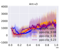
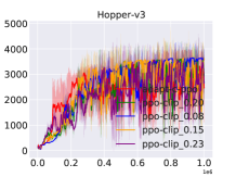
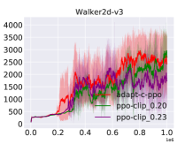
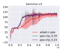
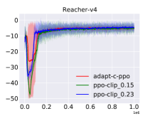
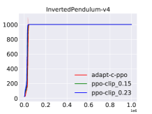
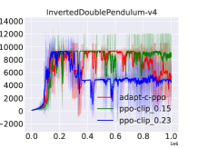
Figure 1 shows the total average evaluation rollouts training for PPO-CLIP and Adaptive-PPO. We repeat at least 3 runs for each tasks, and evaluate every tasks at least 5 times then averaging all runs to plot the training results.

The experimental results indicate that Adaptive-PPO achieves better performance than PPO-CLIP, or it exhibits a faster convergence speed. Specifically, in high-dimensional continuous control tasks such as Ant-V3, Hopper-V3, HalfCheetah-V3, Walker2d-V3, and Humanoid-V3, etc., Adaptive-PPO showed a relatively clear advantage. Meanwhile, in simpler tasks like Swimmer-V3 .etc, Adaptive-PPO performed similarly to PPO-CLIP across all settings. Therefore, dynamically adjusting the clip bound overall allows PPO to achieve better performance. The improvement relative to PPO-CLIP is particularly noticeable in high-dimensional continuous control tasks.

6 Conclusion

In this research, we propose a dynamic adjustment of the PPO surrogate trust region, allowing PPO to dynamically choose a clipping boundary that matches the current state during the optimization process. This enables PPO to achieve stable policy improvement. However, the current work is not yet perfected, and the parameters of our method have not been deliberately turned. Next, we will test the effectiveness of the algorithm from more perspectives and using more tasks.

References

  • Brockman et al. (2016) Brockman, G., Cheung, V., Pettersson, L., Schneider, J., Schulman, J., Tang, J., and Zaremba, W. Openai gym, 2016.
  • Chen et al. (2018) Chen, G., Peng, Y., and Zhang, M. An adaptive clipping approach for proximal policy optimization, 2018.
  • Kakade & Langford (2002) Kakade, S. M. and Langford, J. Approximately optimal approximate reinforcement learning. In International Conference on Machine Learning, 2002. URL https://api.semanticscholar.org/CorpusID:31442909.
  • Lillicrap et al. (2019) Lillicrap, T. P., Hunt, J. J., Pritzel, A., Heess, N., Erez, T., Tassa, Y., Silver, D., and Wierstra, D. Continuous control with deep reinforcement learning, 2019.
  • Mnih et al. (2013) Mnih, V., Kavukcuoglu, K., Silver, D., Graves, A., Antonoglou, I., Wierstra, D., and Riedmiller, M. Playing atari with deep reinforcement learning, 2013.
  • Mnih et al. (2015) Mnih, V., Kavukcuoglu, K., Silver, D., Rusu, A. A., Veness, J., Bellemare, M. G., Graves, A., Riedmiller, M. A., Fidjeland, A. K., Ostrovski, G., Petersen, S., Beattie, C., Sadik, A., Antonoglou, I., King, H., Kumaran, D., Wierstra, D., Legg, S., and Hassabis, D. Human-level control through deep reinforcement learning. Nature, 518:529–533, 2015. URL https://api.semanticscholar.org/CorpusID:205242740.
  • Nahrendra et al. (2023) Nahrendra, I. M. A., Yu, B., and Myung, H. Dreamwaq: Learning robust quadrupedal locomotion with implicit terrain imagination via deep reinforcement learning, 2023.
  • Schulman et al. (2017a) Schulman, J., Levine, S., Moritz, P., Jordan, M. I., and Abbeel, P. Trust region policy optimization, 2017a.
  • Schulman et al. (2017b) Schulman, J., Wolski, F., Dhariwal, P., Radford, A., and Klimov, O. Proximal policy optimization algorithms, 2017b.
  • Schulman et al. (2018) Schulman, J., Moritz, P., Levine, S., Jordan, M., and Abbeel, P. High-dimensional continuous control using generalized advantage estimation, 2018.
  • Yang et al. (2022) Yang, R., Zhang, M., Hansen, N., Xu, H., and Wang, X. Learning vision-guided quadrupedal locomotion end-to-end with cross-modal transformers, 2022.
  • Yu et al. (2022) Yu, C., Velu, A., Vinitsky, E., Gao, J., Wang, Y., Bayen, A., and Wu, Y. The surprising effectiveness of ppo in cooperative, multi-agent games, 2022.
  • Zhuang et al. (2023) Zhuang, Z., Lei, K., Liu, J., Wang, D., and Guo, Y. Behavior proximal policy optimization, 2023.