A survey of the electroweak configuration space and the boson mass
Abstract
Following the recent work of V. Moncrief, A. Marini, R. Maitra [1] and P. Mondal [2] on the geometry of field theoretic configuration spaces, this account examines how the regularized Ricci curvature of the Yang-Mills orbit space may provide an intrinsic mass to the boson which contributes to the value obtained from the renormalized Higgs mechanism. Though the discussion is heuristic, one hopes that this infinite-dimensional technology, which does not postulate extensions to the Standard Model, could explain the mass anomaly reported by the CDF II collaboration.
I Background and geometric motivations
The direct measurement of the boson mass by the CDF II detector [3] has caught many eyes due to its significant deviation from the Standard Model (SM) prediction [4] and results from the ATLAS collaboration [5]. In turn, several theoretical proposals have been made to reconcile the discrepancy albeit by introducing extensions to the SM such as a dark sector [6], a Higgs triplet [7], minimal supersymmetry [8] and more [9, 10, 11, 12, 13, 14, 15, 16]. The call to probe for new physics is strong and exciting, yet it is worth asking whether the apparent anomaly can be explained without any extra ingredients. It is the goal of this presentation to argue for a positive answer to said question by exploring the true origin of mass in gauge theories.
As known, the Higgs mechanism of spontaneous symmetry breaking (SSB) is responsible for endowing the weak bosons with masses at the classical level while keeping renormalizability [17, 18] and gauge invariance of a reduced structure group. However, evidence from perturbation theory in the context of quantum chromodynamics (most notably the phenomenon of asymptotic freedom [19]) seems to point in the direction that quantum Yang-Mills theories with compact semi-simple non-Abelian structure groups over possess a mass gap despite the lack of an explicit mass term in the action pre-SSB. A crude but somewhat supportive case for a mass gap goes as follows. Perturbatively, one breaks the gauge symmetry by splitting the action into a solvable part (consisting of several copies of gauge fields) and then treat the other terms as interactions. According to the Källén–Lehmann representation theorem, the lowest pole in the two-point function for the full theory should give us information about the mass-squared of the first excited state of the Hamiltonian. Let roughly denote the free propagator, then one is unable to yield a mass at any finite order of perturbation since the pole is zero
| (1) |
Keeping in mind issues of convergence, adding all possible terms in the schematic expansion for the 2-point function does give a mass as the pole becomes nonzero
| (2) |
These ideas are of course folly compared to the rigorous demands of constructive quantum field theory [20]. Nevertheless, if existence of quantum Yang-Mills with mass gap proves to be true then it might be possible to give rise to intrinsic masses for the weak bosons in addition to those obtained from the Higgs mechanism. In particular, it is desirable for the intrinsic mass of the to be small enough to account for the CDF II discrepancy. In no way does this presentation intend to tackle the monumental problem of existence of quantum Yang-Mills, rather the result is assumed in order to study the source of mass gap in the electroweak theory by following the analysis of V. Moncrief, A. Marini, R. Maitra [1] and P. Mondal [2].
Begin by recalling the Yang-Mills action on ,
| (3) |
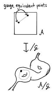
where is a connection of a -bundle over Minkowski space, is the associated curvature 2-form with denoting the coupling, and is a positive-definite adjoint-invariant inner product on the Lie algebra (this is possible since is assumed to be a compact matrix group). If two connections and are defined over the same local trivializing set of , then acting by a transition function (local gauge transformation) yields gauge invariance of the theory . The dynamics of a solution to the field equations is described by a regular curve with prescribed initial conditions living on the phase space. It is important to note that the affine space of spatial connections is not the honest configuration space due to the aforementioned gauge invariance property, instead one must quotient by the group of reduced gauge transformations 111The group includes ordinary gauge transformations as well as those that stabilize a connection i.e. . This gets rid of residual gauge freedom.. Thus, the classical physics takes place in . The nature of this orbit space has been studied throughout the decades [21, 22, 23], it is an infinite-dimensional manifold with incredibly non-trivial topology and moreover it comes equipped with a Riemannian metric induced from the kinetic part of . If we denote coordinates on the base by and the Lie algebra generators by , then the metric takes the following form on the local Coulomb chart around (equivalently, the gauge condition )
| (4) | |||||
with being the structure constants with respect to the chosen basis for and is the gauge covariant Laplacian. The metric is manifest at the level of the action functional as
Note that explicit calculations for the above can be found in [2]. From (4) one can see that is curved (Fig. 1), therefore the canonical quantization procedure will identify the conjugate momentum with times the Levi-Civita covariant derivative on the orbit space (the represents the functional derivative with respect to ). The Hamiltonian is then a formal Laplace-Beltrami operator-valued distribution on plus the potential term
| (5) |
Estimating the spectral gap of becomes tractable as long as one makes suitable assumptions about the quantum Yang-Mills theory, specifically the existence of a normalizable ground state wave functional and a well-behaved weighted measure on the orbit space. This is the content of the work from P. Mondal [2] which was hugely inspired by the intuition of R.P. Feynman who thought that the curvature of the orbit space and the effects of the non-trivial potential might have a bearing on the mass gap [24].
Feynman’s idea was to see the extent to which the gap obtained in 1D particle in a box generalizes to the case of infinite-dimensional geometry. In 1D, the ground state is nodeless and real-positive, which means that the first excited state must contain positive and negative contributions due to orthogonality. This defines a certain “distance” between the positive and negative parts which cannot be arbitrarily large since the potential well forces the quantum mechanical problem to be defined on a compact region of . Because the particle is free inside the box, the excited energy is purely kinetic and must scale as due to the Laplacian. Transitioning to the case of our infinite-dimensional orbit space, the ground state wave functional is presumably nodeless and real-positive due to the potential term being independent of time derivatives of configurations. Taking the ansatz where is real-valued and is a proportionality constant, the normalization condition reads
| (6) |
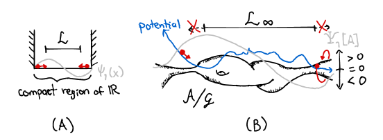
The potential contains quartic terms in the connection as well as lower order combinations which include spatial derivatives, these terms must of course be well-behaved (in a suitable function space setting) for the potential to rise fast enough and yield confinement of . This effect will obviously influence the form of due to the condition (6) which then supplies a weighted measure to . The first excited state must be -orthogonal to , meaning that it must contain orbit space regions where it is positive and other ones where it is negative as in 1D. This property again defines a distance between the positive and negative regions. The question is whether such distance has a finite upper bound, if so then we can be confident in obtaining a gap. However, closed and bounded balls in infinite dimensions fail to be compact, meaning we lose this privilege from the 1D particle in a box. The naive guess is that the distance can be made as large as we want in non-compact directions, but not all hope is lost when we realize that the weighted curved nature of the orbit space can aid in restricting the size of . Indeed, the weighted curvature includes the typical curvature from and effects from the potential made manifest in . As discussed, the potential will tend to confine but it may still admit flat directions and it is at that stage that the curvature contribution solely from will need to step in to restrict . In particular, the desired behavior is obtained when the -Ricci curvature is positive—this makes intuitive sense at least from a pictorial point of view (see Fig. 2) since positivity entails a sort of “converging” behavior. On the other hand, whenever vanishes then we expect to yield the mass gap.
From the standpoint of geometric analysis, these ideas would hint at a generalization of the Lichnerowicz theorem [25, 26] for estimating the first positive eigenvalue of the Laplace-Beltrami operator on compact finite-dimensional manifolds. In the current context, we ditch compactness and finite dimensions and replace the Laplace-Beltrami operator with (5). The finite case requires positivity of Ricci while the orbit space would need positivity of a weighted Ricci which depends on and . The speculations discussed are confirmed by a recent theorem due to P. Mondal [2].
Theorem: Under the assumption of a 1+3 quantized Yang-Mills theory with normalizable ground state , the renormalized Hamiltonian has a mass gap with
| (7) |
as long as the renormalized Bakry–Émery Ricci curvature verifies the following lower bound
| (8) |
for any tangent vector .
A few remarks need to be made about this theorem. First, the notion of renormalized geometry and Hamiltonian is necessary due to the infinite degrees of freedom. In particular, one sees divergence in the metric (4) as and similarly in the operator because the Laplace-Beltrami on is singular already at leading order. [2] introduces a point-split regulator and counterterms to obtain the appropriate finite parts of and , a notable consequence is the emergence of an energy scale via based on dimensional grounds which remains present after renormalization of at the flat connection
| (9) |
where is the Casimir element of the adjoint representation of . The above indicates that must depend on to erase any trail of the regulator and yield a finite result. In other words, becomes a running coupling.
Secondly, Mondal shows via a heat kernel argument that the renormalized Ricci is positive at the flat connection and away from it. Concretely, the inequality is proven. The immediate upshot is that the gap will satisfy contribution) provided the second term is non-negative so that it does not cancel the strictly positive contribution from the Ricci part. There is yet to be a rigorous proof for the non-negativity of the Hessian contribution due to its immense difficulty (specific obstacles are discussed in sections 3 and 6 of [2]), nevertheless explicit computations for the ground state wave functional can be made in the high and low energy limit [27, 28]. In both cases, the Hessian term turns out to be non-negative [29]. Lorentz invariance of the theory would hint at full non-negativity because the potential cannot be independent of the geometrically rich kinetic term, thus the functional must also be ruled by and in turn produce a term of the form ( and a continuous 3-momentum) plus measure zero contributions. This bare-bones claim is motivated by the work of [30, 31] in 1+2 dimensions and [32] in 1+3. For example, [31] found the functional in 1+2 dimensions to be
| (10) |
where is the chromo-magnetic field and is the Laplacian on . The present discussion will take such claim as true and posit the quantity as the classical mass found at the level of the Lagrangian based on the calculations for in solvable theories like Maxwell electromagnetism and the free massive Klein-Gordon theory (see [29] for reference). For the electroweak model, the Hessian contribution to the total mass of the first excited states will be assumed to come solely from the classical Higgs mechanism mass terms whereas the Ricci part will yield intrinsic mass corrections that are quantum in origin (i.e. they cannot be simply inferred from the renormalized Lagrangian but instead one must study the geometry of the electroweak configuration space).
II orbit space of the electroweak bosonic sector
The bosonic sector of the Weinberg-Salam-Glashow electroweak model [33, 34, 35] consist of a Yang-Mills connection with gauge group . The weak isospin and weak hypercharge generators are denoted by and , respectively. At the classical level, all four bosonic fields are massless until a postulated Higgs field transforming in a 2D representation of spontaneously breaks the gauge symmetry by acquiring a nonzero vacuum expectation value. This process retains a smaller symmetry corresponding to electromagnetism which is generated by the hypercharge and the maximal torus of . The Lagrangian then reorganizes itself to yield classical masses to the force carriers that we see in nature
where and are obtained from a rotation in the -plane by a weak mixing angle and are holomorphic and antiholomorphic coordinates in the complexified space. The curvature 2-forms are given by with . Under a action generated by , the physical fields transform as follows
| (12) | |||
and they leave the theory invariant. Based on these considerations, one may extract the metric of the electroweak orbit space from the kinetic part of the action. The Abelian gauge symmetry of the photon implies that the metric will take the form of (4) but without the second term as the structure constants vanish. Similarly, the fact that does not transform at all enforces its orbit space to also be flat
| (13) |
One can immediately conclude the vanishing of the Ricci curvature along the and directions, therefore the total masses for these particles will only be attributed to the Higgs mechanism which is expected to be manifest in the Hessian term of the gap theorem.
A slighter challenge is faced when attempting to compute the metric in the directions due to its non-gauge-like transformation, this will correspond to us obtaining a curved space. Start by reconsidering the theory before SSB and focus on the time component of the Yang-Mills equation with Higgs source
| (14) |
Using the Coulomb gauge condition yields the following formal expression for
| (15) |
The orbit space metric is then extracted from the kinetic term of the action as
One can then leverage (15) to filter through the gauge components of the connections in the last two terms above and hence obtain the non-flat contributions to the orbit space. Observe that the presence of the Higgs source involves time derivatives of and and their mixture with will yield curved contributions to the Higgs field orbit space as well as warped geometry terms to the () spaces. Consequently, the electroweak metric is not decomposable as a “direct sum” of the metrics from each individual space
| (16) |
Furthermore, the fact that the Higgs space is curved will mean that the Higgs boson will receive Ricci contributions to according to the gap theorem. The case is similar for the particles. Even if the source is ignored for ease, the nonflat terms of in the Coulomb chart are still horribly complicated functions of the fields (), their spatial derivatives, and the inverse gauge covariant Laplacian. Note that the decomposition of the metric into flat plus nonflat term would seem to suggest that the Coulomb gauge corresponds to a geodesic normal chart, hence curvature quantities would in principle be determined by explicit computation of the nonflat term. In particular, the task at hand would be to obtain the Ricci tensor and suitably regularize it by means of the point-split method. Once done, positivity would allow us to invoke the gap theorem and obtain the nontrivial intrinsic mass correction to . This in-depth analysis is left for a different time as the main purpose of this short address was to exhibit the ideas of how the mass anomaly might have a resolution via the curvature of the configuration space.
Acknowledgements.
I thank P. Mondal from the Harvard Center of Mathematical Sciences and Applications for many fruitful conversations regarding his gap theorem and the arguments presented here. This project is supported by the Harvard College Research Program.References
- Moncrief et al. [2018] V. Moncrief, A. Marini, and R. Maitra, Orbit space curvature as a source of mass in quantum gauge theory, Annals of Mathematical Sciences and Applications (2018).
- Mondal [2023a] P. Mondal, A Geometric Approach to the Yang-Mills Mass Gap, (2023a), arXiv:2301.06996 [hep-th] .
- CDF Collaboration [2022] CDF Collaboration, High-precision measurement of the W boson mass with the CDF II detector, Science 376(6589), 170–176 (2022).
- Zyla et al. [2020] P. A. Zyla et al. (Particle Data Group), Review of Particle Physics, PTEP 2020, 083C01 (2020).
- ATLAS Collaboration [2023] ATLAS Collaboration, Improved W boson Mass Measurement using = 7 TeV Proton-Proton Collisions with the ATLAS Detector, ATLAS-CONF-2023-004 (2023).
- Zhang and Feng [2023] K.-Y. Zhang and W.-Z. Feng, Explaining the W boson mass anomaly and dark matter with a U(1) dark sector*, Chin. Phys. C 47, 023107 (2023), arXiv:2204.08067 [hep-ph] .
- Kanemura and Yagyu [2022] S. Kanemura and K. Yagyu, Implication of the W boson mass anomaly at CDF II in the Higgs triplet model with a mass difference, Phys. Lett. B 831, 137217 (2022), arXiv:2204.07511 [hep-ph] .
- Rodriguez [2022] M. C. Rodriguez, Explain the -boson mass in the context of the Supersymmetric Model, (2022), arXiv:2209.04653 [hep-ph] .
- Fileviez Perez et al. [2022] P. Fileviez Perez, H. H. Patel, and A. D. Plascencia, On the W mass and new Higgs bosons, Phys. Lett. B 833, 137371 (2022), arXiv:2204.07144 [hep-ph] .
- Krasnikov [2022] N. V. Krasnikov, Nonlocal generalization of the SM as an explanation of recent CDF result, (2022), arXiv:2204.06327 [hep-ph] .
- Nagao et al. [2023] K. I. Nagao, T. Nomura, and H. Okada, A model explaining the new CDF II W boson mass linking to muon and dark matter, Eur. Phys. J. Plus 138, 365 (2023), arXiv:2204.07411 [hep-ph] .
- Lee and Yamashita [2022] H. M. Lee and K. Yamashita, A model of vector-like leptons for the muon and the W boson mass, Eur. Phys. J. C 82, 661 (2022), arXiv:2204.05024 [hep-ph] .
- Bahl et al. [2022] H. Bahl, J. Braathen, and G. Weiglein, New physics effects on the W-boson mass from a doublet extension of the SM Higgs sector, Phys. Lett. B 833, 137295 (2022), arXiv:2204.05269 [hep-ph] .
- Kawamura et al. [2022] J. Kawamura, S. Okawa, and Y. Omura, W boson mass and muon g-2 in a lepton portal dark matter model, Phys. Rev. D 106, 015005 (2022), arXiv:2204.07022 [hep-ph] .
- Yuan et al. [2022] G.-W. Yuan, L. Zu, L. Feng, Y.-F. Cai, and Y.-Z. Fan, Is the W-boson mass enhanced by the axion-like particle, dark photon, or chameleon dark energy?, Sci. China Phys. Mech. Astron. 65, 129512 (2022), arXiv:2204.04183 [hep-ph] .
- Heckman [2022] J. J. Heckman, Extra W-boson mass from a D3-brane, Phys. Lett. B 833, 137387 (2022).
- ’t Hooft and Veltman [1972] G. ’t Hooft and M. J. G. Veltman, Regularization and Renormalization of Gauge Fields, Nucl. Phys. B 44, 189 (1972).
- ’t Hooft [1971] G. ’t Hooft, Renormalizable Lagrangians for Massive Yang-Mills Fields, Nucl. Phys. B 35, 167 (1971).
- Gross and Wilczek [1973] D. J. Gross and F. Wilczek, Ultraviolet Behavior of Nonabelian Gauge Theories, Phys. Rev. Lett. 30, 1343 (1973).
- Jaffe and Witten [2000] A. M. Jaffe and E. Witten, Quantum Yang-Mills theory, (2000).
- I.M. Singer [1981] I.M. Singer, The geometry of the orbit space for non-abelian gauge theories, Physica Scripta, vol. 24, 817 (1981).
- P.K. Mitter and C.M. Viallet [1981] P.K. Mitter and C.M. Viallet, On the bundle of connections and the gauge orbit manifold in Yang-Mills theory, Commun. Math. Phys. 79, 457–472 (1981).
- Babelon and Viallet [1981] O. Babelon and C. M. Viallet, The riemannian geometry of the configuration space of gauge theories, Communications in Mathematical Physics 81, 515 (1981).
- Feynman [1981] R. P. Feynman, The qualitative behavior of yang-mills theory in 2 + 1 dimensions, Nuclear Physics 188, 479 (1981).
- A. Lichnerowicz [1970] A. Lichnerowicz, Variétés riemanniennes à tenseur c non négatif, CR Acad. Sci. Paris Sér. AB, 271, A650-A653 (1970).
- A. Lichnerowicz [1971] A. Lichnerowicz, Variétés kählériennes à première classe de chern non negative et variétés riemanniennes à courbure de ricci généralisée non negative, Journal of Differential Geometry vol. 6, 47-94 (1971).
- B. Hatfield [2018] B. Hatfield, Quantum field theory of point particles and strings, CRC Press (2018).
- Greensite [1979] J. P. Greensite, Calculation of the Yang-Mills vacuum wave functional, Nuclear Physics B 158, 469 (1979).
- Mondal [2023b] P. Mondal, Mass and infinite dimensional geometry, (2023b), arXiv:2308.09304 [hep-th] .
- Nair [2012] V. P. Nair, Quantum effective action, wave functions, and Yang-Mills theory in (2+1) dimensions, Phys. Rev. D 85, 105019 (2012), arXiv:1109.6376 [hep-th] .
- Karabali et al. [1998] D. Karabali, C. Kim, and V. P. Nair, On the vacuum wavefunction and string tension of Yang-Mills theories in (2+1) dimensions, Physics Letters B 434, 103 (1998), arXiv:hep-th/9804132 [hep-th] .
- Mansfield and Sampaio [1999] P. Mansfield and M. Sampaio, Yang-Mills beta-function from a large-distance expansion of the Schrödinger functional, Nuclear Physics B 545, 623 (1999), arXiv:hep-th/9807163 [hep-th] .
- Weinberg [1967] S. Weinberg, A Model of Leptons, Phys. Rev. Lett. 19, 1264 (1967).
- Salam [1968] A. Salam, Weak and Electromagnetic Interactions, Conf. Proc. C 680519, 367 (1968).
- Glashow [1959] S. L. Glashow, The renormalizability of vector meson interactions, Nucl. Phys. 10, 107 (1959).