Bisognano-Wichmann Hamiltonian for the entanglement spectroscopy of fractional quantum Hall states

Abstract

We study the Bisognano-Wichmann Hamiltonian for fractional quantum Hall states defined on a sphere and explore its relationship with the entanglement Hamiltonian associated to the state. We present results for several examples, namely the bosonic Laughlin state stabilized by contact two-body interactions and the bosonic Moore-Read state by either three- or two-body interactions. Our findings demonstrate that the Bisognano-Wichmann Hamiltonian provides a reliable approximation of the entanglement Hamiltonian as a fully-local operator that can be written without any prior knowledge of the specific state under consideration.

Introduction.—Exotic phases of matter exhibiting a fractional quantum Hall (FQH) effect evade the standard paradigm of symmetry breaking [1]. They can instead be classified according to a topological order encoded in the ground state’s patterns of long-range entanglement [2]. Various signatures of topological order have been identified, including a robust ground-state degeneracy [3], the existence of fractionalized excitations [4] the presence of chiral edge-modes [5, 6], and a quantized topological entanglement entropy [7, 8].

In order to gain a deeper understanding of the structure of a FQH state, Li and Haldane emphasized the importance of the spectrum of the reduced density matrix ${\rho}_{A}$, obtained after tracing out any degree of freedom that does not belong to the spatial region $A$. This defines the real-space entanglement Hamiltonian (EH) as

$${H}_{A}=-\log{\rho}_{A},$$ (1)

whose spectrum, also called the real-space entanglement spectrum (RSES), was conjectured to exhibit the same structure as a topological edge mode, suggesting that the spatial partition acts as a virtual edge in the entanglement Hamiltonian [9, 10].

Since measuring the entanglement spectrum presents a considerable experimental challenge [11, 12, 13, 14, 15, 16, 17, 18], an interesting alternative consists in simulating the EH as a physical Hamiltonian defined in subregion $A$. This physical realization of the EH maps the entanglement spectrum to an energy spectrum, which is more easily accessible for experimental measurement [19]. This approach relies on the Bisognano-Wichmann (BW) theorem [20, 21], which provides an explicit form for $H_{A}$ in terms of a local deformation of the original Hamiltonian $H$. By introducing the Hamiltonian density $\mathcal{H}(\mathbf{r})$, such that $H=\int\mathcal{H}(\mathbf{r})d\mathbf{r}$, the exact form of $H_{A}$ reads

$$H^{\rm BW}_{A}=\int_{\mathbf{r}\in A}\beta(\mathbf{r})\mathcal{H}(\mathbf{r})d\mathbf{r},$$ (2)

where the deformation factor $\beta(\mathbf{r})$ is a function of the distance from the partition cut. In the simplest case of a straight-line bipartition, $\beta(\mathbf{r})$ is a linear function of the distance from the cut.

Rigorously proven in the context of Lorentz-invariant local quantum field theories, the BW Hamiltonian ${H}_{A}^{\text{BW}}$ is not generically exact in condensed matter physics [22, 23, 24, 25, 26]. Despite this limitation, it has led to the physical realization of the EH of a non-interacting quantum Hall system with ultracold atomic gases using a synthetic dimension encoded in the internal spin of an atom; in this context, the spatial deformation $\beta(\mathbf{r})$ of the BW Hamiltonian has been engineered through the inhomogeneity of spin couplings [27]. Yet, the use of the BW Hamiltonian to characterize the EH of FQH state in conjunction with the Li-Haldane conjecture has not been addressed so far.

In this article, we study the link between the entanglement Hamiltonian and the BW Hamiltonian for strongly-interacting FQH states. We first show that the BW theorem applies to the single-particle dynamics within the lowest Landau level (LLL). We then focus on systems of bosonic atoms with contact two- or three-body interactions, which are known to exhibit bosonic Laughlin and Moore-Read states. Through a combination of analytical and numerical calculations, we establish that the lowest-energy-branch of the BW Hamiltonian is gapped and matches the conformal-field-theory counting of a topological edge mode. For model wavefunctions, the BW Hamiltonian and the EH share the same eigenvectors, whereas in realistic cases this is true with a high level of accuracy. Overall, our findings provide valuable insights into the spatial entanglement properties of FQH systems.

Single-particle BW Hamiltonian.—Before delving into the FQH interacting problem and the Li-Haldane conjecture, we first focus on the real-space EH for the single-particle problem. To mitigate any edge effects, we conduct our investigations using a spherical geometry. Note that the sphere can be viewed as a compactified plane, and a stereographic projection would allow us to map our results to the planar geometry.

We examine the dynamics of a particle of charge $q$ and mass $M$ as it moves on the surface of a sphere with radius $R$. The particle is subjected to a radial magnetic field $B$ generated by a Dirac magnetic monopole of charge $Q$ positioned at the centre of the sphere. The magnetic flux through the sphere is an integer multiple $2Q\in\mathbb{N}$ of flux quanta $h/q$, so that the magnetic field is $B=\hbar Q/(qR^{2})$. Using the latitude gauge for the vector potential $\mathbf{A}=-\hbar Q/qR\,\cot(\theta){\bm{e}_{\phi}}$, where $(\theta,\phi)$ are the spherical angles, the single particle Hamiltonian reads $H_{0}={\Lambda}^{2}/(2MR^{2})$, with $\mathbf{\Lambda}=\mathbf{R}\times\left(-i\hbar\bm{\nabla}-q\mathbf{A}\right)$ [28, 29].

Owing to rotational symmetry, the eigenstates can be labelled by the angular momentum quantum numbers $L$ and $m$. The spectrum organises in families of degenerate levels, the Landau levels, $E_{L}=\hbar\omega_{c}(L(L+1)-Q^{2})/2Q$, where $\omega_{c}=qB/M$ is the cyclotron frequency, and the angular momentum is restricted to $L=Q+n$ ($n\in\mathbb{N}$). The LLL corresponds to $n=0$ and the single particle wave-functions $\psi_{Q,m}\propto u^{Q+m}v^{Q-m}$ are usually written in terms of spinor variables, $u(\theta,\phi)=\cos(\theta/2)e^{i\phi/2}$ and $v(\theta,\phi)=\sin(\theta/2)e^{-i\phi/2}$, with $-L\leq m\leq L$ [30].

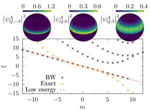
Figure 1: Single-particle RSES $\xi_{A}(m)$ [yellow circles] and spectrum of the BW Hamiltonian in Eq. (3) [black crosses] for a bipartition at the equator and $Q=9$: the lowest branch of the latter spectrum corresponds to the long-wavelength linearized limit of the EH [dashed red line]. The three wavefunctions plotted on top are defined on region $A$ and are eigenfunctions of both the EH and the BW Hamiltonian.

We now consider a bipartition of the sphere into two regions $A$ and $B$, where $A$ corresponds to the northern hemisphere $0\leq\theta\leq\pi/2$. This partition preserves the rotational symmetry around the $z$-axis, so that both the reduced density matrix $\rho_{A}=e^{-H_{A}}$ and the entanglement Hamiltonian $H_{A}$ can be decomposed over spin projections $m$. The EH of the single-particle problem reads $H_{A}=\sum_{m}\xi_{A}(m)\left|\psi^{A}_{Q,m}\right>\left<\psi_{Q,m}^{A}\right|$. The wavefunctions $\psi^{A}_{Q,m}$ are obtained by truncating at $\theta=\pi/2$ and normalising, $\psi_{Q,m}^{A}\propto\psi_{Q,m}\Theta_{\rm H}(\pi/2-\theta)$, where $\Theta_{\rm H}(x)$ is the Heaviside function (see Fig. 1 and [31]). Like in the original LLL, the spin projection $m$ takes integer values in $-L\leq m\leq L$.

Inspired by the BW theorem, we write a BW Hamiltonian for the single-particle problem as

$$H_{A}^{\rm BW}=\frac{4\sqrt{Q}}{\sqrt{\pi}}\,\left\{\frac{H_{0}-\epsilon}{\hbar\omega_{c}},\cos\theta\right\},\quad\text{for }0\leq\theta\leq\frac{\pi}{2}.$$ (3)

The spatial deformation factor $\cos\theta$, which acts as a regularised distance from the equator, is the essence of the BW approach. It disconnects the regions $A$ and $B$, so that it is legitimate to consider the restriction of $H_{A}^{\rm BW}$ to subregion $A$. The anticommutator is required in order to properly define a Hermitian operator, and the energy offset $\epsilon$ reflects the fact that $H_{0}$ is defined up to a constant.

By selecting an energy offset $\epsilon=\hbar\omega_{c}(1+1/2Q)$, which lies midway between the lowest and first excited LL, the truncated LLL wavefunctions $\psi_{Q,m}^{A}$ are exactly the eigenfunctions of the lowest-lying energy band of the BW Hamiltonian in Eq. (3), with eigenvalues

$$\xi^{\rm BW}_{A}(m)=-\frac{4}{\sqrt{\pi\,Q}}\,m,\qquad\text{for }m\leq Q.$$ (4)

The full spectrum of the BW Hamiltonian is plotted in Fig. 1. The lowest band aligns with the EH exact result in the thermodynamic limit ($Q=R^{2}/l_{B}^{2}\to\infty$) [32, 33, 34, 35, 36, 37], thus providing its long-wavelength limit. Note that it extends all the way to $m\to-\infty$, in contrast to the restricted range for the RSES. Indeed, the limitation $m\geq-Q$ for LLL orbitals arises due to divergences at the south pole for $m<-Q$. The BW Hamiltonian $H_{A}^{\rm BW}$, defined on the northern hemisphere only, does not experience this problem. Interestingly, the BW Hamiltonian offers an efficient approach to investigating infinite and precisely linear spectra on finite systems, which may prove useful in various contexts.

This analysis shows that the single-particle EH in the long-wavelength limit can be expressed as a fully local operator. Note that we are not presenting here an effective boundary Hamiltonian, as it has already been discussed [35, 36, 38], but a true bulk Hamiltonian defined on the entire region $A$. Prior to this study, it was not immediately apparent that such a formulation was feasible.

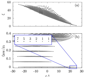
Figure 2: (a) RSES of a bosonic Laughlin state of $N=10$ particles (corresponding to $Q=9$), with $N_{A}=5$. (b) Spectrum of the BW Hamiltonian $\Pi_{\rm BW}V_{A}^{\rm BW}\Pi_{\rm BW}$ for $N_{A}=5$ bosons. The lowest lying zero-energy band has the same degeneracy of the RSES at the same $L_{z}^{A}$. The inset shows a close-up small portion (highlighted by the blue rectangle) of such a band; numbers with the counting of degenerate states have been added for clarity.

BW Hamiltonian for model FQH wavefunctions.—One notable feature of Eq. (3) is that it does not require prior diagonalization of the Hamiltonian $H$ in order to express the BW Hamiltonian $H_{A}^{\rm BW}$. As we will see, this appealing aspect holds true even in the FQH case, where the interactions between particles play a major role.

We now consider the spatial partition of the ground state of $N$ interacting particles evolving on the sphere. The reduced density matrix $\rho_{A}$ (and hence the EH) can be decomposed into symmetry sectors with a fixed number of particles $N_{A}$ and angular momentum $L_{z}^{A}$. In general, the study of the EH in a given sector with $N_{A}$ particles requires computing the ground state for a larger atom number $N>N_{A}$. In contrast, the direct study of the BW Hamiltonian $H_{A}^{\rm BW}$ only requires computing the spectrum for $N_{A}$ particles, which is less computationally demanding.

We begin our investigation by examining the bosonic Laughlin state at filling fraction $\nu=1/2$, which is the exact and gapped ground-state of a two-body contact interaction Hamiltonian $V_{2}(\mathbf{r}_{1},\mathbf{r}_{2})=g_{2}\,\delta^{(2)}(\mathbf{r}_{1}-\mathbf{r}_{2})$ [39, 40, 41]; on the sphere, its stabilization requires $Q=N-1$ [42]. Its RSES, shown in Fig. 2(a), can be characterized by the quantum numbers $N_{A}$ and $L_{z}^{A}$. It consists of a finite branch of states whose counting in the thermodynamic limit corresponds to that of a chiral boson, in agreement with the Li-Haldane conjecture [31, 43, 44, 45, 46, 35, 36, 34].

The generalization of the BW ansatz of Eq. (3) to the many-body case with contact interactions involves a combination of the single-particle Hamiltonian given in Eq. (3) and an interaction term

$$V_{A}^{\rm BW}\!=\!\frac{4\sqrt{Q}}{\sqrt{\pi}}\sum_{i<j}^{N_{A}}\left\{\frac{g_{2}\,\delta(\cos\theta_{i}-\cos\theta_{j})\delta(\phi_{i}-\phi_{j})}{R^{2}\hbar\omega_{c}},\cos\theta_{i}\right\}\!.$$ (5)

In the FQH limit, where the cyclotron energy $\hbar\omega_{c}$ dominates over the interactions, the low-lying features of $H_{A}^{\rm BW}+V_{A}^{\rm BW}$ can be determined using the projector $\Pi_{\rm BW}$ onto the truncated wavefunctions in $\psi_{Q,m}^{A}$, analogously to the standard treatment of FQH effects. Since the BW single-particle Hamiltonian has an exactly linear spectrum, after projection the single-particle BW Hamiltonian becomes trivial: $\Pi_{\rm BW}H_{A}^{\rm BW}\Pi_{\rm BW}=-\frac{4}{\sqrt{\pi Q}}{L_{z}^{A}}$. We thus only focus on the interacting component $\Pi_{\rm BW}V_{A}^{\rm BW}\Pi_{\rm BW}$, and show the results of its numerical diagonalisation in Fig. 2(b) for $N_{A}=5$. A branch of zero-energy states extends up to $L_{z}^{A}=N_{A}(Q+1-N_{A})$, where a single state is seen. This is exactly like the RSES in Fig. 2(a). As we move towards smaller values of $L_{z}^{A}$, the degeneracy of the states increases, precisely matching the expected counting for a chiral boson [47, 31]. To further support this result, we provide exact analytical expressions for the zero-energy eigenstates of $\Pi_{\rm BW}V_{A}^{\rm BW}\Pi_{\rm BW}$ [31], drawing parallels to the well-known construction of excitations in a Laughlin fluid using totally-symmetric polynomials [47]. We can conclude that the interacting BW Hamiltonian exhibits a spectrum with a low-energy branch that satisfies the Li-Haldane conjecture, which proves the interest of performing a quantum simulation of this Hamiltonian.

Note that, for the numerical calculation, the single-particle spectrum, which in principle extends to $m\to-\infty$, is truncated to a finite interval $-Q\leq m\leq Q$. Although the excluded single-particle states could potentially contribute additional zero-energy states to the many-body spectrum, the truncation has no effect on the region $L_{z}^{A}>(N_{A}-2)(Q+1-N_{A})$. Within this interval, our results demonstrate that the subspace spanned by the zero-energy branch of $H_{A}^{\rm BW}$ coincides with the one spanned by the eigenvectors of the EH.

In practice, the experimental implementation of spatially-deformed interactions as given by Eq. 5 may be challenging. However, the fact that the relevant many-body states of the BW Hamiltonian have zero interaction energy makes the spatial deformation unnecessary. We have verified this by examining the case of pure contact interactions $V_{2}$, finding the same zero-energy band of Fig. 2(b), but a different excited-band structures. [31].

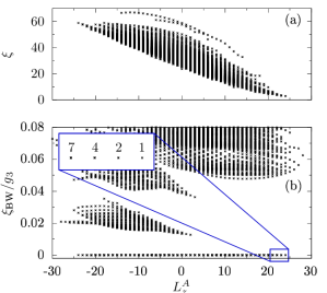
Figure 3: (a) RSES of a bosonic Moore-Read state of $N=14$ particles (corresponding to $Q=6$), with $N_{A}=7$. (b) Spectrum of the projected BW Hamiltonian $V$ for $N_{A}=7$ bosons, without the linear dispersion term (Eq. (3)), in the case of three-body contact interactions $V_{3}$. The lowest lying zero-energy band has the same degeneracy of the RSES at the same $L_{z}^{A}$. The inset shows a close-up small portion (highlighted by the blue rectangle) of such a band; numbers with the counting of degenerate states have been added for clarity.

Next, we consider the bosonic Moore-Read state at filling $\nu=1$ as a second case study. This state corresponds to the exact ground state of a three-body contact interaction $V_{3}(\mathbf{r}_{1},\mathbf{r}_{2},\mathbf{r}_{3})=g_{3}\,\delta^{(2)}(\mathbf{r}_{1}-\mathbf{r}_{2})\delta^{(2)}(\mathbf{r}_{1}-\mathbf{r}_{3})$ [48, 49, 50]. On the sphere, its stabilization requires $2Q=N-2$ [42]. The extension of the BW Hamiltonian to the contact three-body interaction is straightforward. In this case as well, the interacting BW Hamiltonian exhibits a zero-energy band that shares the same eigenvector structure as the exact entanglement Hamiltonian (see Fig. 3). In agreement with the Li-Haldane conjecture, the state degeneracies matches the edge conformal field theory, which consists for the Moore-Read state of a chiral boson and a chiral fermion [31].

BW Hamiltonian for numerical FQH states.—The exactness of the results presented so far for analytically-known model wavefunctions opens up the question on whether the BW Hamiltonian can be used to study the RSES of generic FQH states. In this final section we present a positive answer by considering the state in the Moore-Read phase stabilized by two-body contact interactions [51, 42, 52, 41, 53]–a state relevant for cold-atom experiments [54] that cannot be expressed analytically.

Figure 4: (a) RSES ($N_{A}=7$) of a state of $N=14$ bosons, $Q=6$, stabilized by two-body contact interactions $V_{2}$, which is expected to be in the Moore-Read universality class. (b) Spectrum of the BW Hamiltonian $\Pi_{\rm BW}V_{A}^{\rm BW}\Pi_{\rm BW}$ for $N_{A}=7$ bosons. In both cases the points have been coloured according to the expectation value of the three-body contact interaction $V_{3}$. For clarity reasons an arbitrary linear dispersion term has been introduced in the BW case.

It has been shown that the RSES of this state, plotted in Fig. 4(a), displays a low-lying branch analogous to that of the analytical Moore-Read state in Fig. 3(a), as well as a novel high-lying branch [55]. While the two branches are separated at low energy they merge at higher energy, limiting the identification of the levels that belong to the low-energy branch.In the specific example of Fig. 4(a), we are able to unequivocally isolate the ground energy branch for 7 values of $L_{z}^{A}$, from $18$ to $24$.

We now compare this entanglement spectrum with the energy spectrum of the corresponding BW Hamiltonian, shown in Fig. 4(b). Just like the RSES, a single state emerges at angular momentum $L_{z}^{A}=24$. As we move towards lower angular momentum states, we observe the development of a branch with the same number of states as the RSES, namely $\{1,2,4\}$ from right to left. This branch eventually merges at angular momentum $L_{z}^{A}=21$ with the high-lying branch. We conclude that, even for this non-model wavefunction, the low-energy spectrum of the BW Hamiltonian reproduces the Li-Haldane conjecture. In the SM we present additional numerical results for different bipartitions, highlighting the even-odd $N_{A}$ effect on the edge-state counting [31].

We also compare the eigenvectors of the EH and BW Hamiltonians. We first consider the expectation value of the three-body contact interaction potential $V_{3}$, which is encoded in the colour of the markers of Fig. 4. This local observable quantifies the characteristic three-body anti-bunching expected in the Moore-Read state. This observable takes very similar values in both EH and BW Hamiltonians, and a more detailed comparison is presented in [31], demonstrating relative differences of a few percent points. We also computed the overlap matrix [56] between the EH and BW Hamiltonian eigenvectors, within the low-energy branch, at fixed quantum numbers $N_{A}$ and $L_{z}^{A}$. We expect this matrix to describe a change of basis if the BW Hamiltonian captures the EH physics. We found a unitary matrix at the $10^{-3}$ level [31]. We thus conclude that the EH and BW Hamiltonians can be approximately put in direct correspondance in their low-energy branch.

Conclusions.—We have revisited the fundamental problem of the RSES of FQH states proposing a study based on the BW Hamiltonian; our results show that it correctly captures the features of the entanglement Hamiltonian, satisfying several properties among which the Li-Haldane conjecture. These positive results open the exciting perspective of establishing an accurate mathematical connection beyond the numerical results that we have presented.

A remarkable result is that the BW Hamiltonian can be constructed straightforwardly from the knowledge of the physical Hamiltonian only, without the need of computing the ground state to be studied. This in particular means that one does not even need to know what specific form of topological order is displayed by the ground state, which is typically necessary for constructing the EH as an effective boundary conformal field theory. For this reason, we expect the BW Hamiltonian to become a useful tool in numerical studies.

Finally, given the recent realisation of a non-interacting BW Hamiltonian in a cold-atom quantum simulator, this work opens new paths in the experimental study of the RSES of the paradigmatic topological phases of the FQH effects.

Acknowledgements.—We acknowledge fruitful discussions with N. Regnault. We thank I. Carusotto for careful reading of the manuscript. This work is supported by European Union (grants TOPODY 756722 (Paris) and LoCoMacro 805252 (Orsay) from the European Research Council) and by Region Ile-de-France in the framework of the DIM Sirteq. M. R. acknowledges support by the Deutsche Forschungsgemeinschaft (DFG) with project Grant No. 277101999 within the CRC network TR 183 (subproject B01) and under Germany’s Excellence Strategy - Cluster of Excellence Matter and Light for Quantum Computing (ML4Q) EXC 2004/1 - 390534769. A. N. acknowledges support by Fondazione Angelo dalla Riccia and thanks LPTMS for warm hospitality. S. N. acknowledges support from Institut Universitaire de France.

Supplemental Materials to
Bisognano-Wichmann Hamiltonian for the entanglement spectroscopy
of fractional quantum Hall states A. Nardin

R. Lopes

M. Rizzi

L. Mazza

S. Nascimbene

I Lowest band of the single-particle Bisognano-Wichmann Hamiltonian

In this first section we show that the sharply-truncated lowest Landau level wavefunctions on the sphere are eigenvectors of the Bisognano-Wichmann Hamiltonian. In this supplemental materials, we discuss a general latitude angle $\theta_{0}$ for the bipartition, whereas in the main text we focused only on the half-bipartition of the sphere, $\theta_{0}=\pi/2$.

We rewrite the Bisognano-Wichmann Hamiltonian as

$$H_{BW}=\frac{4}{\sqrt{\pi\,Q}}\left\{\frac{H_{0}-\epsilon}{\hbar\omega_{c}},\mathcal{F}(\theta)\right\},\qquad\text{with}\quad 0\leq\theta\leq\theta_{0}\quad\text{and}\quad\mathcal{F}(\theta)=Q(\cos(\theta)-\cos(\theta_{0}))\geq 0;$$ (6)

the coordinates are restricted to the upper spherical cap and we introduced the function $\mathcal{F}(\theta)$ measuring the distance from the bipartition cut. In the fractional quantum Hall context, this distance function can interpreted as measuring the “orbital-distance” between lowest-Landau level orbitals on the sphere, which are peaked at $\cos(\theta_{M})=M/Q$. Notice that such a form appeared previously in Ref. [57] within a different context.

Here $\epsilon$ is in principle an arbitrary energy shift, which we will choose by requiring the lowest Landau level truncated wavefunctions to be eigenfunction of the Bisognano-Wichmann Hamiltonian, and $H_{0}$ is the free single particle Hamiltonian [29]

$$H_{0}=\frac{|\mathbf{\Lambda}|^{2}}{2MR^{2}}=\frac{\hbar\omega_{c}}{2Q}\left(-\frac{1}{\sin(\theta)}\frac{\partial}{\partial\theta}\sin(\theta)\frac{\partial}{\partial\theta}+\left(Q\cot(\theta)+\frac{i}{\sin(\theta)}\frac{\partial}{\partial\phi}\right)^{2}\right).$$ (7)

The (normalized) eigenvectors of $H_{0}$ are so-called monopole harmonics [29, 58, 59]

$$Y_{Q,l,m}=\sqrt{\frac{2l+1}{4\pi}\,\frac{(l-m)!}{(l-Q)!}\frac{(l+m)!}{(l+Q)!}}\,2^{-m}\,(1-\cos(\theta))^{\frac{-Q+m}{2}}(1+\cos(\theta))^{\frac{Q+m}{2}}\,P_{l-m}^{-Q+m,Q+m}(\cos(\theta))e^{im\phi},$$ (8)

where $P_{n}^{(\alpha,\beta)}(x)=2^{-n}\sum_{s=0}^{n}\binom{n+\alpha}{s}\binom{n+\beta}{n-s}(x-1)^{n-s}(x+1)^{s}$ are the Jacobi polynomials. Here, $2Q\in\mathbb{Z}$ is the flux through the sphere, $l\geq Q$ is the total angular momentum eigenvalue and $-l\leq m\leq l$ the eigenvalue of its projection along the $z$ axis. The eigenvalue associated to $Y_{Q,l,m}$ is $E_{Q,l}=\hbar\omega_{c}\frac{l(l+1)-Q^{2}}{2Q}$; the lowest Landau level corresponds to $l=|Q|$, i.e. $E_{Q,Q}=\frac{1}{2}\hbar\omega_{c}$.

The action of $H_{BW}$ on these states can be computed

$$\frac{H_{BW}}{4/\sqrt{\pi Q}}Y_{Q,l,m}=\frac{1}{2Q}\left(-\frac{\partial^{2}\mathcal{F}}{\partial\theta^{2}}Y_{Q,l,m}-2\frac{\partial\mathcal{F}}{\partial\theta}\,\frac{\partial Y_{Q,l,m}}{\partial\theta}-\frac{\cos(\theta)}{\sin(\theta)}\frac{\partial\mathcal{F}}{\partial\theta}Y_{Q,l,m}\right)+2\mathcal{F}\left(\frac{l(l+1)-Q^{2}}{2Q}-\frac{\epsilon}{\hbar\omega_{c}}\right)Y_{Q,l,m}.$$ (9)

Notice that introducing Heaviside theta functions in the monopole harmonics (i.e. restricting them to the proper Bisognano-Wichmann domain) does not (as can be checked explicitly) change the above equation since the two domains $\theta>\theta_{0}$ and $\theta<\theta_{0}$ are disconnected by $\mathcal{F}(\theta)$, i.e. $\mathcal{F}(\theta_{0})=0$. Provided we set $\epsilon=\hbar\omega_{c}\frac{2Q+1}{2Q}$ (midway between the lowest LL $E_{Q,Q}$ and the first LL $E_{Q,Q+1}$), it is easy to check (to this purpose, see Eq. (29)) that $Y_{Q,Q,m}$ (the lowest-Landau level wavefunctions with $l=Q$) are eigenvectors

$$H_{BW}Y_{Q,Q,m}=-\frac{4}{\sqrt{\pi Q}}\left(m-(Q+1)\cos(\theta_{0})\right)Y_{Q,Q,m}.$$ (10)

Analogously to lowest Landau level wavefunctions on the sphere, the normalized eigenvectors of the Bisognano-Wichmann Hamiltonian are most simply written in terms of spinor-variables $u(\theta,\phi)=\cos(\theta/2)e^{i\phi/2}$ and $v(\theta,\phi)=\sin(\theta/2)e^{-i\phi/2}$ as

$$\psi_{Q,m}^{A}=\frac{u^{Q+m}(\theta,\phi)v^{Q-m}(\theta,\phi)}{\sqrt{4\pi\mathrm{B}_{\sin^{2}\left(\frac{\theta_{0}}{2}\right)}(Q+1-m,Q+1+m)}}\Theta_{\rm H}(\theta_{0}-\theta),$$ (11)

where $\mathrm{B}_{x}(a,b)$ is the incomplete Beta function, $\mathrm{B}_{x}(a,b)=\int_{0}^{x}t^{a-1}(1-t)^{b-1}\,dt$. Notice that we introduced the Heaviside theta function $\Theta_{\rm H}(\theta_{0}-\theta)$, which sharply separates the two spherical caps.

II Single-particle entanglement spectrum

In this section we analytically describe the structure of the entanglement Hamiltonian in the case of a single-particle state occupying a well defined orbital $Y_{Q,Q,m}$ in the lowest Landau level. The reduced density matrix can be decomposed as

$$\rho_{A}=\left(1-\mathcal{N}_{A}\right)\left|v_{A}\right>\left<v_{A}\right|+\mathcal{N}_{A}\left|\psi_{A}\right>\left<\psi_{A}\right|$$ (12)

where $A$ is the spherical cap defined by $\theta<\theta_{0}$, $\left|v_{A}\right>$ is the state with no particles in $A$ and $\psi_{A}$ the one with a single particle restricted to this region. Finally

$$\mathcal{N}_{A}=\int d\phi\int_{0}^{\theta_{0}}\sin(\theta)d\theta\,|Y_{Q,Q,m}|^{2}=\frac{\mathrm{B}_{\sin^{2}\left(\theta_{0}/2\right)}\left(Q+1-m,Q+1+m\right)}{\mathrm{B}(Q+1-m,Q+1+m)}.$$ (13)

Here, $\mathrm{B}(a,b)=\mathrm{B}_{1}(a,b)$ is the Beta function. Since the particle either is the $A$ region or it is not, the entanglement Hamiltonian, defined by $\rho_{A}=e^{-H_{A}}/\text{Tr}[e^{-H_{A}}]$, can be written as

$$H_{A}=E_{v_{A}}\left|v_{A}\right>\left<v_{A}\right|+E_{\psi_{A}}\left|\psi_{A}\right>\left<\psi_{A}\right|$$ (14)

with $E_{v_{A}}$ and $E_{\psi_{A}}$ being dimensionless quantities. With some algebra it can be shown that the previous relations are compatible provided

$$\mathcal{N}_{A}=\frac{1}{2}\left[1-\tanh\left(\frac{E_{\psi_{A}}-E_{v_{A}}}{2}\right)\right]$$ (15)

which characterizes the entanglement energies up to a global additive constant, which can be fixed by requiring $E_{v_{A}}=0$.

Inverting Eq. (15) and using Eq. (13) we get

$$\begin{split}E_{\psi_{A}}=&-2\text{atanh}\left(2\mathcal{N}_{A}-1\right)\\ =&-2\,\text{atanh}\left(2\,\frac{\mathrm{B}_{\sin^{2}\left(\theta_{0}/2\right)}\left(Q+1-m,Q+1+m\right)}{\mathrm{B}(Q+1-m,Q+1+m)}-1\right).\end{split}$$ (16)

When $\theta_{0}=\pi/2$, Eq. (13) can be linearized for $m/Q\ll 1$ using the Beta function integral representation and Laplace’s method, yielding

$$\mathcal{N}_{A}\approx\frac{1}{2}+\frac{m}{\sqrt{\pi Q}}$$ (17)

which, when inserted in Eq. (16) gives

$$E_{\psi_{A}}\approx-\frac{4m}{\sqrt{\pi Q}}=-\frac{4\,kl_{B}}{\sqrt{\pi}}.$$ (18)

where the momentum $k=\frac{2\pi}{\mathcal{C}}\,m$ and $\mathcal{C}=2\pi R$ is the length of the bipartition cut. This last expression is the same one can find for an integer quantum Hall system on the plane [37], which is locally indistinguishable from a sphere when its radius goes to infinity.

III Diagonalization of the single-particle Bisognano-Wichmann Hamiltonian

In this section, we detail how the full spectrum of the Bisognano-Wichmann Hamiltonian is obtained.

We begin by introducing $\lambda_{Q,l}=l(l+1)-Q^{2}-(2Q+1)$ and rewriting Eq. (9) as

$$\frac{H_{BW}}{4/\sqrt{\pi Q}}Y_{Q,l,m}=(\lambda_{Q,l}+1)\,\cos(\theta)Y_{Q,l,m}+\sin(\theta)\,\frac{\partial Y_{Q,l,m}}{\partial\theta}-\lambda_{Q,l}\cos(\theta_{0})Y_{Q,l,m}.$$ (19)

We now want to diagonalize $H_{BW}$ by expanding its general eigenvector on the basis provided by the monopole harmonics. With the choice of bipartition $\mathcal{F}=\mathcal{F}(\theta)$ (independent of $\phi$), the $z$-projection of the angular momentum is still a good quantum number. We can therefore write

$$H_{BW}\Psi_{Q,\alpha,m}=E_{Q,\alpha,m}\Psi_{Q,\alpha,m}$$ (20)

and expand

$$\Psi_{Q,\alpha,m}=\sum_{l}C_{l,\alpha}^{Q,m}Y_{Q,l,m}.$$ (21)

multiplying by $Y^{*}_{Q,l^{\prime},m}$ and integrating over the spherical cap $A$ we are considering we end up with a generalized eigenvalue problem (the states $Y_{Q,l,m}$ are not normalized nor orthogonal on the bipartition)

$$\sum_{l}\mathcal{H}_{l^{\prime},l}^{Q,m}C_{l,\alpha}^{Q,m}=E_{Q,\alpha,m}\sum_{l}\mathcal{M}_{l^{\prime},l}^{Q,m}C_{l,\alpha}^{Q,m}$$ (22)

where

$$\begin{cases}\mathcal{H}_{l^{\prime},l}^{Q,m}=\int_{A}Y^{*}_{Q,l^{\prime},m}H_{BW}Y_{Q,l,m}d\Omega\\ \mathcal{M}_{l^{\prime},l}^{Q,m}=\int_{A}Y^{*}_{Q,l^{\prime},m}Y_{Q,l,m}d\Omega.\end{cases}$$ (23)

The integrals could be performed numerically, but it is not difficult to express them as finite summations, which allow for a more straightforward numerical evaluation. We here sketch the calculation of these matrix elements, giving only the main results.

The integration over the region $A$ can be seen as an integral over the whole space with a characteristic function $\Theta_{\rm H}(\theta_{0}-\theta)$ which can be expanded in terms of monopole harmonics

$$\begin{cases}\Theta_{\rm H}(\theta_{0}-\theta)=\sum_{l}\zeta_{l}Y_{0,l,0}\\ \zeta_{l}=2\pi\sqrt{\frac{2l+1}{4\pi}}\,\frac{P_{l-1}(\cos(\theta_{0})-P_{l+1}(\cos(\theta_{0}))}{2l+1}\end{cases}$$ (24)

where $P_{n}(x)$ are Legendre polynomials. Products of monopole harmonics can be simplified in terms of Wigner 3j symbols [59]

$$\begin{split}Y_{Q,l,m}Y_{Q^{\prime},l^{\prime},m^{\prime}}=&\sum_{l^{\prime\prime}}(-1)^{l+l^{\prime}+l^{\prime\prime}}(-1)^{Q+Q^{\prime}}(-1)^{m+m^{\prime}}\sqrt{\frac{(2l+1)(2l^{\prime}+1)(2l^{\prime\prime}+1)}{4\pi}}\,\\ &\begin{pmatrix}l&l^{\prime}&l^{\prime\prime}\\ m&m^{\prime}&-(m+m^{\prime})\end{pmatrix}\begin{pmatrix}l&l^{\prime}&l^{\prime\prime}\\ Q&Q^{\prime}&-(Q+Q^{\prime})\end{pmatrix}Y_{Q+Q^{\prime},l^{\prime\prime},m+m^{\prime}}\end{split}$$ (25)

and as a consequence of orthonormality integrals involving three of them can be written as [59]

$$\int Y_{Q,l,m}Y_{Q^{\prime},l^{\prime},m^{\prime}}Y_{Q^{\prime\prime},l^{\prime\prime},m^{\prime\prime}}d\Omega=(-1)^{l+l^{\prime}+l^{\prime\prime}}\sqrt{\frac{(2l+1)(2l^{\prime}+1)(2l^{\prime\prime}+1)}{4\pi}}\,\begin{pmatrix}l&l^{\prime}&l^{\prime\prime}\\ -m&-m^{\prime}&-m^{\prime\prime}\end{pmatrix}\begin{pmatrix}l&l^{\prime}&l^{\prime\prime}\\ Q&Q^{\prime}&Q^{\prime\prime}\end{pmatrix}.$$ (26)

Using $Y^{*}_{Q,l,m}=(-1)^{Q-m}Y_{Q,l,m}$ [59], the overlaps matrix elements can be written as

$$\mathcal{M}_{l^{\prime},l}^{Q,m}=(-1)^{Q-m}\sum_{l^{\prime\prime}=|l^{\prime}-l|}^{l+l^{\prime}}\zeta_{l^{\prime\prime}}(-1)^{l+l^{\prime}+l^{\prime\prime}}\sqrt{\frac{(2l+1)(2l^{\prime}+1)(2l^{\prime\prime}+1)}{4\pi}}\,\begin{pmatrix}l&l^{\prime}&l^{\prime\prime}\\ -m&m&0\end{pmatrix}\begin{pmatrix}l&l^{\prime}&l^{\prime\prime}\\ Q&-Q&0\end{pmatrix}.$$ (27)

Using $\cos(\theta)=\sqrt{\frac{4\pi}{3}}Y_{0,1,0}$ together with Eq. (25) and Eq. (26), the first integral appearing inside $\mathcal{H}_{l,l^{\prime}}^{Q,m}$ can be calculated

$$\begin{split}I_{l^{\prime},l}^{Q,m}=\int_{A}Y^{*}_{Q,l^{\prime},m}\cos(\theta)Y_{Q,l,m}d\Omega=&(-1)^{Q-m}\sum_{l^{\prime\prime\prime}=|l^{\prime}-l|}^{l+l^{\prime}}(2l^{\prime\prime\prime}+1)\begin{pmatrix}l&l^{\prime}&l^{\prime\prime\prime}\\ -m&m&0\end{pmatrix}\begin{pmatrix}l&l^{\prime}&l^{\prime\prime\prime}\\ Q&-Q&0\end{pmatrix}\\ &\sum_{l^{\prime\prime}=|l^{\prime\prime\prime}-1|}^{l^{\prime\prime\prime}+1}(-1)^{1+l+l^{\prime}+l^{\prime\prime}}\zeta_{l^{\prime\prime}}\sqrt{\frac{(2l+1)(2l^{\prime}+1)(2l^{\prime\prime}+1)}{4\pi}}\begin{pmatrix}1&l^{\prime\prime\prime}&l^{\prime\prime}\\ 0&0&0\end{pmatrix}^{2}.\end{split}$$ (28)

Using the results of Ref. [60] it is not difficult to show that

$$\sin(\theta)\,\frac{\partial Y_{Q,l,m}}{\partial\theta}=\left(l\cos(\theta)-\frac{Q}{l}m\right)Y_{Q,l,m}-\frac{1}{l}\sqrt{\frac{2l+1}{2l-1}(l^{2}-m^{2})(l^{2}-Q^{2})}\,\,Y_{Q,l-1,m}.$$ (29)

The only contribution to $\mathcal{H}_{l,l^{\prime}}^{Q,m}$ with a functional form different from the ones already analysed is seen to be

$$\begin{split}J_{l^{\prime},l}^{Q,m}=\int_{A}Y^{*}_{Q,l^{\prime},m}Y_{Q,l-1,m}d\Omega=&(-1)^{Q-m}\sum_{l^{\prime\prime}=|l-l^{\prime}-1|}^{l+l^{\prime}-1}\zeta_{l^{\prime\prime}}(-1)^{l-1+l^{\prime}+l^{\prime\prime}}\sqrt{\frac{(2l-1)(2l^{\prime}+1)(2l^{\prime\prime}+1)}{4\pi}}\,\\ &\begin{pmatrix}l-1&l^{\prime}&l^{\prime\prime}\\ -m&m&0\end{pmatrix}\begin{pmatrix}l-1&l^{\prime}&l^{\prime\prime}\\ Q&-Q&0\end{pmatrix}.\end{split}$$ (30)

Therefore, putting everything together we get

$$\begin{split}\frac{\mathcal{H}_{l^{\prime},l}^{Q,m}}{4/\sqrt{\pi Q}}=&\int_{A}Y^{*}_{Q,l^{\prime},m}H_{BW}Y_{Q,l,m}d\Omega=(\lambda_{Q,l}+1)\,I_{l^{\prime},l}^{Q,m}+\left(l\,I_{l^{\prime},l}^{Q,m}-\frac{Q}{l}m\,\mathcal{M}_{l^{\prime},l}^{Q,m}\right)-\\ &\frac{1}{l}\sqrt{\frac{2l+1}{2l-1}(l^{2}-m^{2})(l^{2}-Q^{2})}\,\,J_{l^{\prime},l}^{Q,m}-\lambda_{Q,l}\cos(\theta_{0})\,\mathcal{M}_{l^{\prime},l}^{Q,m}.\end{split}$$ (31)

The matrix elements of both the Bisognano-Wichmann Hamiltonian $\mathcal{H}_{l^{\prime},l}^{Q,m}$ and the overlaps matrix $\mathcal{M}_{l^{\prime},l}^{Q,m}$ are henceforth obtained from Eq. (31), Eq. (28), Eq. (30) and Eq. (27); the generalized eigenvalue problem Eq. (22) can then be numerically solved.

Notice that the ground-band (see Eq. (10)) can be recovered in this formalism by setting $C_{l,\alpha_{gb}}^{Q,m}\propto\delta_{l,Q}$, meaning that $\Psi_{Q,\alpha_{gb},m}\propto Y_{Q,Q,m}$. This ansatz is indeed a valid solution for the generalized eigenvalue problem Eq. (22)

$$\mathcal{H}_{l^{\prime},Q}^{Q,m}=E_{Q,\alpha_{gb},m}\mathcal{M}_{l^{\prime},Q}^{Q,m}$$ (32)

provided $E_{Q,\alpha_{gb},m}$ are those given by Eq. (10). Indeed after setting $l=Q$, the Hamiltonian matrix elements Eq. (31) simplify considerably

$$\frac{\mathcal{H}_{l^{\prime},Q}^{Q,m}}{4/\sqrt{\pi Q}}=-\left(m-(Q+1)\cos(\theta_{0})\right)\,\mathcal{M}_{l^{\prime},Q}^{Q,m}$$ (33)

leading to

$$E_{Q,\alpha_{gb},m}=-\frac{4}{\sqrt{\pi Q}}\left(m-(Q+1)\cos(\theta_{0})\right)$$ (34)

which as anticipated matches Eq. (10).

IV Diagonalization of the many-particles Bisognano-Wichmann Hamiltonian

In this section we briefly detail how the many-body problem has been diagonalized. We consider, as we did in the main text, the two- and three- body contact interaction $V_{2}(\mathbf{r}_{i},\mathbf{r}_{j})=g_{2}\delta^{(2)}(\mathbf{r}_{i}-\mathbf{r}_{j})$ and $V_{3}(\mathbf{r}_{i},\mathbf{r}_{j},\mathbf{r}_{k})=g_{3}\delta^{(2)}(\mathbf{r}_{i}-\mathbf{r}_{j})\delta^{(2)}(\mathbf{r}_{i}-\mathbf{r}_{k})$. The spatially deformed Bisognano-Wichmann interactions read

$$V_{A,2}^{\rm BW} =\frac{8\sqrt{Q}}{\sqrt{\pi}}\,\frac{g_{2}}{R^{2}\hbar\omega_{c}}\,\frac{\delta(\theta_{i}-\theta_{j})}{\sin(\theta_{i})}\delta(\phi_{i}-\phi_{j})\,\left(\cos(\theta_{i})-\cos(\theta_{0})\right)$$ (35)

$$V_{A,3}^{\rm BW} =\frac{8\sqrt{Q}}{\sqrt{\pi}}\,\frac{g_{3}}{R^{4}\hbar\omega_{c}}\,\frac{\delta(\theta_{i}-\theta_{j})}{\sin(\theta_{i})}\frac{\delta(\theta_{i}-\theta_{k})}{\sin(\theta_{i})}\delta(\phi_{i}-\phi_{j})\delta(\phi_{i}-\phi_{k})\,\left(\cos(\theta_{i})-\cos(\theta_{0})\right).$$ (36)

Since the magnetic field is assumed to be large, we project these deformed interactions onto the lowest level of the Bisognano-Wichmann Hamiltonian, Eq. (11). In second-quantization language the deformed interaction Hamiltonian therefore reads

$$\Pi_{\rm BW}V_{A,2}^{\rm BW}\Pi_{\rm BW} =\frac{1}{2!}\sum_{\begin{subarray}{c}m_{1},m_{2}\\ m_{3},m_{4}\end{subarray}}\left<m_{1},m_{2}\right|V_{2}\left|m_{3},m_{4}\right>\,a^{\dagger}_{m_{1}}a^{\dagger}_{m_{2}}a^{\vphantom{\dagger}}_{m_{3}}a^{\vphantom{\dagger}}_{m_{4}}$$ (37)

$$\Pi_{\rm BW}V_{A,3}^{\rm BW}\Pi_{\rm BW} =\frac{1}{3!}\sum_{\begin{subarray}{c}m_{1},m_{2},m_{3}\\ m_{4},m_{5},m_{6}\end{subarray}}\left<m_{1},m_{2},m_{3}\right|V_{3}\left|m_{4},m_{5},m_{6}\right>\,a^{\dagger}_{m_{1}}a^{\dagger}_{m_{2}}a^{\dagger}_{m_{3}}a^{\vphantom{\dagger}}_{m_{4}}a^{\vphantom{\dagger}}_{m_{5}}a^{\vphantom{\dagger}}_{m_{6}}$$ (38)

where $\left|m\right>=a^{\dagger}_{m}\left|0\right>$ and $a^{\dagger}_{m}$ creates a particle with angular momentum $m$ in the lowest-lying band of the Bisognano-Wichmann Hamiltonian; namely, $\left<\mathbf{r}|m\right>=\psi_{Q,m}^{A}(\mathbf{r})$ (see Eq. (11)). Since we consider bosons, annihilation/creation operators at the same angular momentum do not commute and rather obey $[a^{\vphantom{\dagger}}_{m},a^{\dagger}_{m^{\prime}}]=\delta_{m,m^{\prime}}$.

The relevant matrix elements can be computed explicitly as

$$\left<m_{1},m_{2}\right|V_{2}\left|m_{3},m_{4}\right> =\frac{8\sqrt{Q}}{\sqrt{\pi}}\,\frac{g_{2}}{R^{2}\hbar\omega_{c}}\,\frac{\delta_{m_{1}+m_{2},m_{3}+m_{4}}\,F_{\sin^{2}(\theta_{0}/2)}\left(Q,\frac{m_{1}+m_{2}+m_{3}+m_{4}}{2}\right)}{4\pi\sqrt{\prod_{i=1}^{4}\mathrm{B}_{\sin^{2}(\theta_{0}/2)}\left(Q+1-m_{i},Q+1+m_{i}\right)}}$$ (39)

$$\left<m_{1},m_{2},m_{3}\right|V_{3}\left|m_{4},m_{5},m_{6}\right> =\frac{8\sqrt{Q}}{\sqrt{\pi}}\,\frac{g_{3}}{R^{4}\hbar\omega_{c}}\,\frac{\delta_{m_{1}+m_{2}+m_{3},m_{4}+m_{5}+m_{6}}\,G_{\sin^{2}(\theta_{0}/2)}\left(Q,\frac{m_{1}+m_{2}+m_{3}+m_{4}+m_{5}+m_{6}}{2}\right)}{(4\pi)^{2}\sqrt{\prod_{i=1}^{6}\mathrm{B}_{\sin^{2}(\theta_{0}/2)}\left(Q+1-m_{i},Q+1+m_{i}\right)}}$$ (40)

where

$$\begin{split}F_{x}\left(Q,M\right)=\mathrm{B}_{x}\left(2Q-M+1,2Q+M+3\right)&-\mathrm{B}_{x}\left(2Q-M+3,2Q+M+1\right)-\\ &-\cos(\theta_{0})\,\mathrm{B}_{x}\left(2Q-M+1,2Q+M+1\right)\end{split}$$ (41)

and

$$\begin{split}G_{x}\left(Q,M\right)=\mathrm{B}_{x}\left(3Q-M+1,3Q+M+3\right)&-\mathrm{B}_{x}\left(3Q-M+3,3Q+M+1\right)-\\ &-\cos(\theta_{0})\,\mathrm{B}_{x}\left(3Q-M+1,3Q+M+1\right).\end{split}$$ (42)

Using standard exact diagonalization techniques the projected Bisognano-Wichmann interaction Hamiltonians given by Eq. (37) and Eq. (38) can then be diagonalized.

Figure 5: Deviations from unitarity of the matrix of overlaps between real-space entanglement Hamiltonian eigenvectors with finite entanglement energy and the Bisognano-Wichmann Hamiltonian eigenvectors lying below the entanglement gap. The image on the left is for the case of a bosonic Laughlin state with $N=10$ particles ($Q=9$), bipartitioned at the equator in two equal hemispheres ($N_{A}=5$, $\theta_{0}=\pi/2$). The image on the right is for the case of a bosonic Moore-Read state with $N=14$ particles ($Q=6$), bipartitioned at the equator in two equal hemispheres ($N_{A}=7$, $\theta_{0}=\pi/2$).

V Exact zero-energy eigenstates of the Bisognano-Wichmann Hamiltonian for the Laughlin state

In this section, we analytically write down the eigenstates of the many-body Bisognano-Wichmann in the case of the projected two-body contact interaction, $\Pi_{\rm BW}V_{A}^{\rm BW}\Pi_{\rm BW}$. It is not difficult in this case to write down the analytical expressions for the zero-energy eigenstates of the Bisognano-Wichmann Hamiltonian, using the fact that the single-particle levels are restricted to the lowest Bisognano-Wichmann band. We stereographically project the sphere onto the complex plane $z_{i}=2R\,v_{i}/u_{i}=2R\,\tan(\theta_{i}/2)e^{-i\phi_{i}}$ [61]. We require that the many-body wavefunction has the good symmetry for a system of $N_{A}$ bosons, and that each particle sees a wavefunction-zero at the position of the other ones. In this case the many-body states will lie in the kernel of the interaction Hamiltonian. We can therefore mimic the well-known construction of excitations in a Laughlin fluid [47], by writing

$$\Psi(\{z_{i}\})\sim\Phi(\{z_{i}\})\,\,\prod_{i<j}(z_{i}-z_{j})^{2}\,\prod_{i}\,\frac{\Theta_{\rm H}\left(\tan\left(\frac{\theta_{0}}{2}\right)-\frac{|z_{i}|}{2R}\right)}{\left(1+\frac{|z_{i}|^{2}}{4R^{2}}\right)^{1+Q}}.$$ (43)

Here the Heaviside function comes from the restriction of the $N_{A}$ particles to the northern spherical cap, and $\Phi(\{z_{i}\})$ is a symmetric polynomial of homogeneous degree $\ell$. If, as we did in the main text, we restrict to truncated wavefunctions with $-Q\leq m\leq Q$, the maximal degree at which each $z_{i}$ can appear must be positive and cannot exceed $2Q-2(N_{A}-1)$. In each angular momentum sector $L_{z}^{A}$, the counting of these polynomials exactly matches the one of the real-space entanglement spectrum at fixed $N_{A}$ and $L_{z}^{A}$, and in the scaling limit approaches the chiral-boson one. It is important to notice that these states exactly match the eigenvectors of the real-space entanglement Hamiltonian.

On the other hand, if the full Bisognano-Wichmann lowest lying band is considered, there is no such constraint on the degree of $\Phi(\{z_{i}\})$. The two countings will be the same provided $\ell\leq 2(Q+1-N_{A})$, i.e. $L_{z}^{A}>(N_{A}-2)(Q+1-N_{A})$.

We numerically verified that the vector-space spanned by these eigenvectors at fixed $N_{A}$, $L_{z}^{A}$ spans exactly the same vector-space spanned by the eigenvectors of the entanglement Hamiltonian having finite entanglement energy. We did so by computing the matrix of overlaps between the eigenvectors $\left|\psi^{\rm BW}_{i}\right>$ of the Bisognano-Wichmann Hamiltonian those of the entanglement one, $\left|\phi^{\rm RSES}_{\alpha}\right>$. We then tested whether such a matrix represented a change of basis by testing its unitarity computing the Hilbert-Schmidt norm of $\mathcal{O}^{\dagger}\mathcal{O}^{\vphantom{\dagger}}-\mathbb{1}$. The results are shown in Fig. 5. It can be seen that, to numerical accuracy, the two set of eigenvectors indeed span the same vector-subspace.

VI Contact two-body interaction as a proxy for the Bisognano-Wichmann Hamiltonian

From the previous section it is clear that, since the relevant many-body states of the Bisognano-Wichmann Hamiltonian have zero interaction-energy, the spatial deformation associated to the Bisognano-Wichmann interaction Hamiltonian is not necessary when dealing with model wavefunctions. This simple observation is highly relevant for quantum-simulation platforms, where in practice the experimental implementation of spatially-deformed interactions is not straightforward: provided the deformed single particle Bisognano-Wichmann can be implemented, the “bare” two- or three-body interactions will stabilize states which correspond to the eigenstates of the entanglement Hamiltonian of a Laughlin and Moore-Read state, respectively.

This is illustrated in Fig. 6, both for the case of the Laughlin (left panel) and Moore-Read (right panel) states. Even though the excited (non-zero energy) states in the two cases are different (and notice that the Bisognano-Wichmann Hamiltonian makes the entanglement gap larger), the zero-energy branch shares exactly the same eigenvectors (and therefore it exhibits the same state counting).

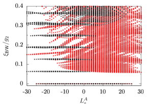
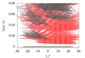
Figure 6: The images compare the spectra of the original interaction (red circles) with the Bisognano-Wichmann one (black crosses) projected onto the lowest branch of the single-particle Bisognano-Wichmann Hamiltonian, for the two cases of contact two-body interactions at $N=10$ and $Q=9$ (left image) and contact three-body ones at $N=14$ and $Q=6$ (right image). The two cases mimic the entanglement Hamiltonian of the Laughlin and Moore-Read states, respectively.

VII State counting

Before discussing the analysis we performed for the case of non-model wavefunctions, in this section we briefly review the counting of edge modes for the two topological orders we analysed, the Laughlin and the Moore-Read states.

Laughlin edge-states counting

A simple physical way of accounting for the edge excitations of a Laughlin state is the hydrodynamical approach. This fractional quantum Hall state can be seen as a single-component incompressible fluid, which contains no low-energy bulk excitations. On the other hand, gapless chiral modes are localized at the system’s boundary. These surface deformations at low-energy and long-wavelengths can be completely described by a $\text{U}(1)$ Kac-Moody algebra [47]

$$\begin{array}[]{l}H=\frac{2\pi}{L}\hbar\frac{v}{\nu}\sum_{k>0}\rho_{-k}\,\rho_{k}\\ \left[\rho_{k},\rho_{-k^{\prime}}\right]=\nu\frac{kL}{2\pi}\,\delta_{k,k^{\prime}}\end{array}$$ (44)

where $\rho_{k}$ are the modes of the 1-dimensional density at the edge of the system. We consider a compact edge of length $L$ and label the momentum $k=\frac{2\pi}{L}\,n$ by an integer $n$. The edge of a Laughlin state can therefore be described by a bosonic field theory, with the Laughlin ground state being the vacuum of the theory $\left|0\right>$. The modes at a given momentum $K$ can then be written as $\prod_{n\in\bm{\lambda}}a^{\dagger}_{n}\left|0\right>$, where $\bm{\lambda}$ is an integer partition of $K/(2\pi/L)\equiv M$ and $a^{\dagger}_{n}\propto\rho_{-k}$. We list the lowest lying excitations in Table 1.

Momentum $\Delta M$	Partition $\bm{\lambda}$	States	Number of states	Energy $\Delta E$
$0$	$\{\}$	$\left|0\right>$	1	$0$
$1$	$\{1\}$	$a^{\dagger}_{1}\left|0\right>$	1	$e_{0}$
$2$	$\{2\}$	$a_{2}^{\dagger}\left|0\right>$	2	$2e_{0}$
	$\{1,1\}$	$(a^{\dagger}_{1})^{2}\left|0\right>$
$3$	$\{3\}$	$a_{3}^{\dagger}\left|0\right>$	3	$3e_{0}$
	$\{2,1\}$	$a_{2}^{\dagger}a_{1}^{\dagger}\left|0\right>$
	$\{1,1,1\}$	$(a_{1}^{\dagger})^{3}\left|0\right>$
$4$	$\{4\}$	$a_{4}^{\dagger}\left|0\right>$	5	$4e_{0}$
	$\{3,1\}$	$a_{3}^{\dagger}a_{1}^{\dagger}\left|0\right>$
	$\{2,2\}$	$(a_{2}^{\dagger})^{2}\left|0\right>$
	$\{2,1,1\}$	$a_{2}^{\dagger}(a_{1}^{\dagger})^{2}\left|0\right>$
	$\{1,1,1,1\}$	$(a_{1}^{\dagger})^{4}\left|0\right>$

Table 1: List of the lowest lying edge excitations on top of the Laughlin ground state. We defined $e_{0}=v\,\hbar\frac{2\pi}{L}$. Momentum and energy are measured with respect to the one of the ground state, $\left|0\right>$.

Moore-Read edge-states counting

The edge excitations of the Moore-Read state contain, in addition to the $\text{U}(1)$ Kac-Moody algebra associated to a branch of bosonic edge excitations analogous to the one of the Laughlin liquid described above, a chiral Majorana fermion [62, 63], which can have both periodic or anti-periodic boundary conditions. The low-energy and long-wavelength description of this mode reads

$$\begin{array}[]{l}H=\frac{2\pi}{L}\,\hbar v^{\prime}\sum_{n\geq 0}n\,c_{-n}\,c_{n}\\ \left\{c_{n},c_{-n^{\prime}}\right\}=\delta_{n,n^{\prime}},\end{array}$$ (45)

where $n-\frac{1}{2}\in\mathbb{N}$ ($n\in\mathbb{N}$) for anti-periodic (periodic) boundary conditions on the fermion field. The edge-excitations of the Moore-Read ground state turn out to correspond to the choice of anti-periodic boundary conditions. The theory has two additional independent sectors, according to the (conserved) parity of the number of fermions excited along the edge. This parity has to match the one of the number of electrons in the system. We list the lowest lying excitations in Table 3 and 3.

Momentum $\Delta M$ States Number of states Energy $\Delta E$ $0$ $\left|0\right>$ 1 $0$ $1$ 0 $e_{0}^{\prime}$ $2$ $c_{3/2}c_{1/2}\left|0\right>$ 1 $2e_{0}^{\prime}$ $3$ $c_{5/2}c_{1/2}\left|0\right>$ 1 $3e_{0}^{\prime}$ $4$ $c_{7/2}c_{1/2}\left|0\right>$ 2 $4e_{0}^{\prime}$ $c_{5/2}c_{3/2}\left|0\right>$ Table 2: List of the lowest lying edge excitations of a Majorana fermion with antiperiodic boundary conditions and even number of fermions. We defined $e_{0}^{\prime}=\hbar v^{\prime}\,\frac{2\pi}{L}$. Momentum and energy are measured with respect to the zero-momentum ground state, $\left|0\right>$. Momentum $\Delta M$ States Number of states Energy $\Delta E$ $0$ $c_{1/2}\left|0\right>$ 1 $0$ $1$ $c_{3/2}\left|0\right>$ 1 $e_{0}^{\prime}$ $2$ $c_{5/2}\left|0\right>$ 1 $2e_{0}^{\prime}$ $3$ $c_{7/2}\left|0\right>$ 1 $3e_{0}^{\prime}$ $4$ $c_{9/2}\left|0\right>$ 2 $4e_{0}^{\prime}$ $c_{5/2}c_{3/2}c_{1/2}\left|0\right>$ Table 3: List of the lowest lying edge excitations of a Majorana fermion with antiperiodic boundary conditions and odd number of fermions. We defined $e_{0}^{\prime}=\hbar v^{\prime}\,\frac{2\pi}{L}$. Momentum and energy are measured with respect to the ground state, $c_{1/2}\left|0\right>$.

The total number of excitations of the Moore-Read state is then obtained by taking the product between the Majorana fermion sector and the bosonic charge sector. We list the number of degeneracies in Table 5 with a few selected examples for the states at $\Delta M=3$ in Table 5.

Momentum $\Delta M$ Number of states (even $N$) Number of states (odd $N$) $0$ 1 1 $1$ 1 2 $2$ 3 4 $3$ 5 7 $4$ 10 13 Table 4: Number of gapless edge modes at the boundary of a Moore-Read topological order with either even or odd particle numbers, $N$. Momentum $\Delta M$ States (even $N$) States (odd $N$) 3 $a_{3}^{\dagger}\left|0\right>$ $a_{3}^{\dagger}c^{\vphantom{\dagger}}_{1/2}\left|0\right>$ $a_{2}^{\dagger}a_{1}^{\dagger}\left|0\right>$ $a_{2}^{\dagger}a_{1}^{\dagger}c^{\vphantom{\dagger}}_{1/2}\left|0\right>$ $(a_{1}^{\dagger})^{3}\left|0\right>$ $(a_{1}^{\dagger})^{3}c^{\vphantom{\dagger}}_{1/2}\left|0\right>$ $a_{1}^{\dagger}c^{\vphantom{\dagger}}_{5/2}c^{\vphantom{\dagger}}_{1/2}\left|0\right>$ $a_{2}^{\dagger}c^{\vphantom{\dagger}}_{3/2}\left|0\right>$ $c_{5/2}^{\vphantom{\dagger}}c_{1/2}^{\vphantom{\dagger}}\left|0\right>$ $(a_{1}^{\dagger})^{2}c^{\vphantom{\dagger}}_{3/2}\left|0\right>$ $a_{1}^{\dagger}c^{\vphantom{\dagger}}_{5/2}\left|0\right>$ $c^{\vphantom{\dagger}}_{7/2}\left|0\right>$ Table 5: Edge-states of a Moore-Read topological order with either even or odd particle numbers, $N$ in the $\Delta M=3$ momentum sector.

VIII Numerical analysis for the contact interacting Moore-Read state

In this final section we present additional numerical data for the relevant case of the Moore-Read topological order stabilized by two-body contact interactions. We start by discussing bipartitions with particles numbers $N_{A}\neq N/2$, which allow us to investigate more thoroughly the connection between the Bisognano-Wichamann and the real-space entanglement Hamiltonian. We then show that the eigenvectors of the Bisognano-Wichmann Hamiltonian are, to a good level of approximation, the same as those of the real-space entanglement spectrum, thereby proving the validity of the Bisognano-Wichmann ansatz.

Spherical-cap bipartition

We here introduce a new cut in order to extensively study the connection between the Bisognano-Wichmann ansatz and the real-space entanglement Hamiltonian as a function not only of the particle number $N$, but also as a function of the bipartition particle number sector $N_{A}$. A natural choice is to move the longitudinal bipartition, so that the probability of having $N_{A}$ particles within the spherical cap defined by $0\leq\theta\leq\theta_{0}$ (see the insets of Fig. 7) does not change drastically as $N_{A}$ is varied.

Such an angle can be determined by the following simple physical consideration. A fractional quantum Hall ground state is an incompressible featureless liquid which in the thermodynamic limit has uniform density $\rho_{0}=\nu/2\pi l_{B}^{2}$, where $\nu$ is the filling fraction and $l_{B}=\sqrt{\hbar/qB}$ the magnetic length. We require

$$N_{A}=\int_{0}^{2\pi}R\,d\phi\int_{0}^{\theta_{0}}R\sin(\theta)d\theta\,\rho_{0}$$ (46)

i.e. that the number of particles in the spherical-cap is precisely $N_{A}$. Since $R^{2}/l_{B}^{2}=Q$, this leads to $N_{A}=2\nu Q\sin^{2}\left(\frac{\theta_{0}}{2}\right)$. Since $2Q=N_{\phi}=\nu^{-1}N-\mathcal{S}\approx\nu^{-1}N$ ($\mathcal{S}$ being the so-called “shift” [64]) we finally get

$$\theta_{0}=2\arcsin\sqrt{\frac{N_{A}}{N}}.$$ (47)

In the following, we will vary the cut longitude $\theta_{0}$ with $N$ and $N_{A}$ as prescribed by the relation Eq. (47). Notice that with this choice the length $\mathcal{L}$ of the cut does not change as the number of particles $N$ is increased and $N_{A}$ is kept constant, for $\mathcal{L}=2\pi R\sin(\theta_{0})\approx\pi\sqrt{N_{A}/\nu}\,l_{B}$.

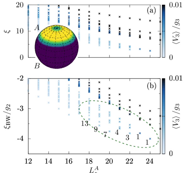
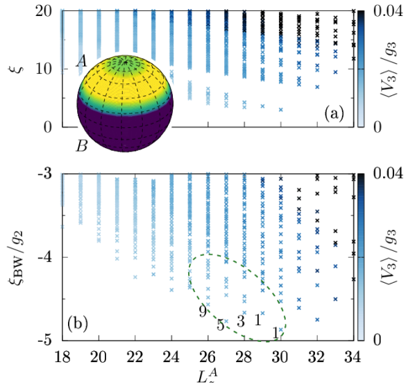
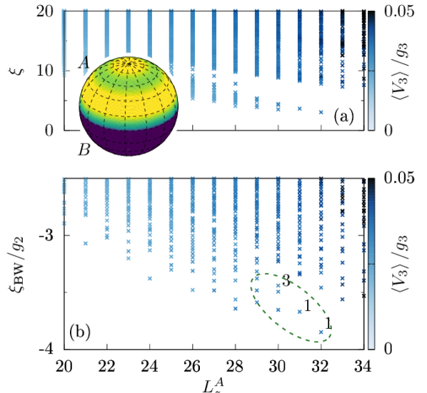
Figure 7: The three images show the real-space entanglement spectra for $N=16$, $Q=7$ bosonic Moore-Read state at filling $\nu=1$, stabilized by two-body contact interactions (panels (a)), compared to the Bisognano-Wichmann ansatz for the given bipartiton (panels (b)), which, from left to right, are given by $N_{A}=4,6,8$. In the lower panel, the dashed elliptical shape serves as a guide to the eye for the lower branch of states and the numbers indicate the number of states it comprises at a given $L_{z}^{A}$, for the values that are in agreement with the real-space entanglement spectrum. The insets show the density of the lowest-lying state of the Bisognano-Wichmann Hamiltonian as a heat-map, illustrating how the spherical cap at longitude $\theta_{0}$ is varied as a function of $N_{A}$. In all cases the points have been coloured according to the expectation value of the three-body contact interaction $V_{3}$. For clarity reasons an arbitrary linear dispersion term has been introduced in the Bisognano-Wichmann case.

Comparisons between the real-space entanglement spectrum and the Bisognano-Wichmann one are presented in Fig. 7 for $N=16$, $Q=7$ and three different values of $N_{A}=4,6,8$. The cuts at different values of $\theta_{0}$ are clearly visible in the insets, which display the ground-state density of the Bisognano-Wichmann Hamiltonian.

More importantly, it can be seen that the counting of the lowest lying Bisognano-Wichmann states matches the one of the real-space entanglement spectrum. In particular, these plots complement the data presented in the main text, where we considered $N_{A}$ to be odd: it can be seen that for both the even and odd cases the Bisognano-Wichmann Hamiltonian reproduces the correct counting for a Moore-Read topological order, and that these value approach the conformal field theory countings.

It can be noted moreover that the Li-Haldane counting for smaller values of $N_{A}$ extends to smaller values of $L_{z}^{A}$, covering a larger region. Furthermore, the Bisognano-Wichmann entanglement gap looks to be more robust for smaller $N_{A}$. We do not have an explanation for this behaviour, which deserves further investigation.

Finally it can be seen that the expectation values of the three-body contact interaction (plotted as a colour-scale) computed using the real-space entanglement Hamiltonian eigenvectors and the Bisognano-Wichmann ones are in qualitative agreement. In the case of the “entanglement ground-state”, we verified the relative error committed by the Bisognano-Wichmann ansatz is within some percent points, see Fig. 8. We did not analyse states at different values of $L_{z}^{A}$, because the analysis is complicated by the presence of additional states at the same value of $L_{z}^{A}$ which can in principle mix among each other.

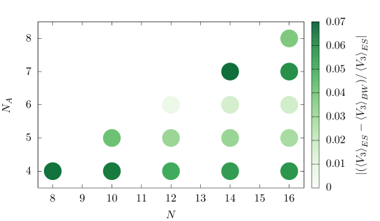
Figure 8: Absolute value of the relative error on the expectation value of the three-body contact interaction computed using either the eigenvectors of the real space entanglement Hamiltonian or the Bisognano-Wichmann one, in the case of a bosonic $\nu=1$ Moore-Read-like phase at $2Q=N-2$ stabilized by two-body contact interactions. On the $x$-axis, various values for the number of particles $N$ (which fix the value of $Q$) are shown, while on the $y$-axis we plot various values for the particles $N_{A}$ in the northern spherical-cap.

Overlaps

We already discussed that in the case of model wavefunctions the eigenvectors of the Bisognano-Wichmann Hamiltonian are the same as those of the real-space entanglement one. One does not expect this to be true in general for non-model states. Therefore, a relevant question which we address here is to what extent the eigenvectors $\left|\psi^{\rm BW}_{i}\right>$ of the Bisognano-Wichmann Hamiltonian provide a good description of those of the entanglement one, $\left|\phi^{\rm RSES}_{\alpha}\right>$.

Instead of blindly computing the overlaps between eigenvectors, as already discussed above we study the matrix of the overlaps $\mathcal{O}_{\alpha,i}=\left<\phi^{\rm RSES}_{\alpha}|\psi^{\rm BW}_{i}\right>$ as a function of $N_{A}$ and $L_{z}^{A}$; we already discussed in the main text that, at least for a certain range of values of $L_{z}^{A}$, the counting of states below the so-called “entanglement-gap” match for the two approaches, satisfying the Li-Haldane conjecture. As a consequence, the overlap matrix $\mathcal{O}$ restricted to such a subspace is a square matrix, which we expect to be unitary if the Bisognano-Wichmann Hamiltonian captures the same features as the entanglement one. In particular this means that the two low-entanglement-energy subspaces are expected to span the same vector subspace within the whole Hilbert space.

To test the unitarity we compute the (normalized) Hilbert-Schmidt norm of $\delta=\mathcal{O}^{\dagger}\mathcal{O}^{\vphantom{\dagger}}-\mathbb{1}$

$$||\delta||=\frac{1}{d}\,\sum_{i,j}^{d}|\delta_{i,j}|^{2}$$ (48)

where the sum runs over the $d^{2}$ coefficients of the difference matrix $\delta$, namely the Li-Haldane counting of the low-entanglement-energy modes. Normalizing by $d$ ensures that $||\mathbb{1}||=1$, i.e. that the identity has unit norm. Moreover, it accounts for finite-size effects in the Li-Haldane counting: at fixed $N_{A}$ and $L_{z}^{A}$, the conformal field theory counting is recovered only when $N\rightarrow\infty$.

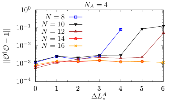
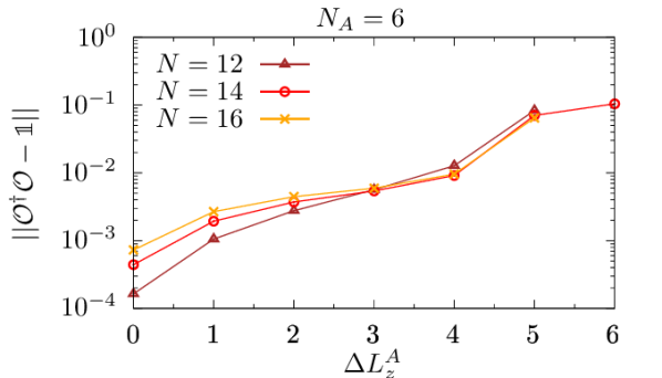
Figure 9: Deviations from unitarity of the matrix of overlaps between real-space entanglement and Bisognano-Wichmann Hamiltonian eigenvectors lying below the entanglement gap. Data are presented as a function of the angular-momentum variation $\Delta L_{z}^{A}$ with respect to the one of the entanglement Hamiltonian ground state, for different values of the number of particles $N$ (which fix the value of the flux through the sphere, $2Q=N-2$). The image on the left considers $N_{A}=4$ particles in the northern spherical cap, the one on the right $N_{A}=6$.

The results are presented in Fig. 9 for $N_{A}=4$ and $N_{A}=6$, for different values of $L_{z}^{A}$ measured with respect to the “entanglement ground-state” value. It can be seen that the Bisognano-Wichmann Hamiltonian provides indeed a good description of the entanglement structure of fractional quantum Hall ground states, even away from the model-wavefunctions limit. No apparent scaling is visible, though. A possible reason could lie in the choice of the spherical geometry, which was chosen so as to avoid edge effects, but may be affected by Gaussian curvature effects. The analysis of a planar geometry, which is free of curvature effects but may be plagued by edge ones, is reserved for a future study. A second possibility could be that a system sufficiently large so that the long-wavelength regime in which the Bisognano-Wichmann can be expected to give better results was not reached with the small sizes exact-diagonalization puts at our disposal. A hint of this fact can be seen even in the density plots in Fig. 7, where density oscillations at the bipartition cut prevent the bulk from reaching the incompressible “featureless” limit $\rho_{0}$. Finally, a third possibility could be rooted in the fact that overlaps are not well defined in the thermodynamic limit, even though the proper long-wavelength features of the topological order have been captured. This would actually be analogous to what happens for model wavefunctions: their overlap with “real” topologically ordered ground states is expected to drop to zero in the thermodynamic limit, even if the model wavefunction captures all of its essential details. A better indicator could be to analyse expectation values of local observables, analogously to what was done in Fig. 8, but this again is reserved for future more systematic studies.

References

- Wen [2017] X.-G. Wen, Colloquium: Zoo of quantum-topological phases of matter, Rev. Mod. Phys. 89, 041004 (2017).
- Chen et al. [2010] X. Chen, Z.-C. Gu, and X.-G. Wen, Local unitary transformation, long-range quantum entanglement, wave function renormalization, and topological order, Phys. Rev. B 82, 155138 (2010).
- Wen [1990] X. G. Wen, Topological orders in rigid states, Int. J. Mod. Phys. B 04, 239 (1990).
- Laughlin [1983] R. B. Laughlin, Anomalous quantum hall effect: An incompressible quantum fluid with fractionally charged excitations, Phys. Rev. Lett. 50, 1395 (1983).
- Wen [1991] X. G. Wen, Gapless boundary excitations in the quantum hall states and in the chiral spin states, Phys. Rev. B 43, 11025 (1991).
- Chang [2003] A. M. Chang, Chiral luttinger liquids at the fractional quantum hall edge, Rev. Mod. Phys. 75, 1449 (2003).
- Levin and Wen [2006] M. Levin and X.-G. Wen, Detecting Topological Order in a Ground State Wave Function, Phys. Rev. Lett. 96, 110405 (2006).
- Kitaev and Preskill [2006] A. Kitaev and J. Preskill, Topological Entanglement Entropy, Phys. Rev. Lett. 96, 110404 (2006).
- Li and Haldane [2008a] H. Li and F. D. M. Haldane, Entanglement spectrum as a generalization of entanglement entropy: Identification of topological order in non-abelian fractional quantum hall effect states, Phys. Rev. Lett. 101, 010504 (2008a).
- Regnault [2017] N. Regnault, Entanglement spectroscopy and its application to the quantum Hall effects, Lecture Notes Les Houches Summer School 103, 165 (2017).
- Dalmonte et al. [2022] M. Dalmonte, V. Eisler, M. Falconi, and B. Vermersch, Entanglement Hamiltonians: From Field Theory to Lattice Models and Experiments, Ann. Phys. 534, 2200064 (2022).
- Choo et al. [2018] K. Choo, C. W. von Keyserlingk, N. Regnault, and T. Neupert, Measurement of the Entanglement Spectrum of a Symmetry-Protected Topological State Using the IBM Quantum Computer, Phys. Rev. Lett. 121, 086808 (2018).
- Sankar et al. [2023] S. Sankar, E. Sela, and C. Han, Measuring topological entanglement entropy using maxwell relations, Phys. Rev. Lett. 131, 016601 (2023).
- Pichler et al. [2016] H. Pichler, G. Zhu, A. Seif, P. Zoller, and M. Hafezi, Measurement Protocol for the Entanglement Spectrum of Cold Atoms, Phys. Rev. X 6, 041033 (2016).
- Johri et al. [2017] S. Johri, D. S. Steiger, and M. Troyer, Entanglement spectroscopy on a quantum computer, Phys. Rev. B 96, 195136 (2017).
- Beverland et al. [2018] M. E. Beverland, J. Haah, G. Alagic, G. K. Campbell, A. M. Rey, and A. V. Gorshkov, Spectrum Estimation of Density Operators with Alkaline-Earth Atoms, Phys. Rev. Lett. 120, 025301 (2018).
- Kokail et al. [2021a] C. Kokail, R. van Bijnen, A. Elben, B. Vermersch, and P. Zoller, Entanglement Hamiltonian tomography in quantum simulation, Nat. Phys. 17, 936 (2021a).
- Joshi et al. [2023] M. K. Joshi, C. Kokail, R. van Bijnen, F. Kranzl, T. V. Zache, R. Blatt, C. F. Roos, and P. Zoller, Exploring large-scale entanglement in quantum simulation, Nature 10.1038/s41586-023-06768-0 (2023).
- Dalmonte et al. [2018] M. Dalmonte, B. Vermersch, and P. Zoller, Quantum simulation and spectroscopy of entanglement Hamiltonians, Nat. Phys. 14, 827 (2018).
- Bisognano and Wichmann [1975] J. J. Bisognano and E. H. Wichmann, On the duality condition for a Hermitian scalar field, J. Math. Phys. 16, 985 (1975).
- Bisognano and Wichmann [1976] J. J. Bisognano and E. H. Wichmann, On the duality condition for quantum fields, J. Math. Phys. 17, 303 (1976).
- Giudici et al. [2018] G. Giudici, T. Mendes-Santos, P. Calabrese, and M. Dalmonte, Entanglement Hamiltonians of lattice models via the Bisognano-Wichmann theorem, Phys. Rev. B 98, 134403 (2018).
- Mendes-Santos et al. [2019] T. Mendes-Santos, G. Giudici, M. Dalmonte, and M. A. Rajabpour, Entanglement Hamiltonian of quantum critical chains and conformal field theories, Phys. Rev. B 100, 155122 (2019).
- Zhang et al. [2020] J. Zhang, P. Calabrese, M. Dalmonte, and M. A. Rajabpour, Lattice Bisognano-Wichmann modular Hamiltonian in critical quantum spin chains, SciPost Phys. Core 2, 007 (2020).
- Kokail et al. [2021b] C. Kokail, B. Sundar, T. V. Zache, A. Elben, B. Vermersch, M. Dalmonte, R. van Bijnen, and P. Zoller, Quantum Variational Learning of the Entanglement Hamiltonian, Phys. Rev. Lett. 127, 170501 (2021b).
- Zache et al. [2022] T. V. Zache, C. Kokail, B. Sundar, and P. Zoller, Entanglement Spectroscopy and probing the Li-Haldane Conjecture in Topological Quantum Matter, Quantum 6, 702 (2022).
- Redon et al. [2023] Q. Redon, Q. Liu, J.-B. Bouhiron, N. Mittal, A. Fabre, R. Lopes, and S. Nascimbene, Realizing the entanglement Hamiltonian of a topological quantum Hall system, arXiv:2307.06251 (2023).
- Greiter [2011] M. Greiter, Landau level quantization on the sphere, Phys. Rev. B 83, 115129 (2011).
- Jain [2007] J. K. Jain, Composite Fermions (Cambridge University Press, 2007).
- Haldane and Rezayi [1985] F. D. M. Haldane and E. H. Rezayi, Finite-size studies of the incompressible state of the fractionally quantized hall effect and its excitations, Phys. Rev. Lett. 54, 237 (1985).
- Note [1] See Supplemental Material for the eigenvalues and eigenvectors of the single-particle entanglement Hamiltonian, the analytical expressions for the eigenstates of zero interaction energy of the BW Hamiltonian, the many-body spectrum of the BW Hamiltonian with uniform contact interactions, a detailed comparison between EH and BW Hamiltonians for the numerical Moore-Read state, and a detailed explanation of the CFT edge mode counting for Laughlin and Moore-Read states.
- Rodríguez and Sierra [2009] I. D. Rodríguez and G. Sierra, Entanglement entropy of integer quantum hall states, Phys. Rev. B 80, 153303 (2009).
- Rodríguez et al. [2012] I. D. Rodríguez, S. H. Simon, and J. K. Slingerland, Evaluation of ranks of real space and particle entanglement spectra for large systems, Phys. Rev. Lett. 108, 256806 (2012).
- Sterdyniak et al. [2012] A. Sterdyniak, A. Chandran, N. Regnault, B. A. Bernevig, and P. Bonderson, Real-space entanglement spectrum of quantum hall states, Phys. Rev. B 85, 125308 (2012).
- Dubail et al. [2012a] J. Dubail, N. Read, and E. H. Rezayi, Real-space entanglement spectrum of quantum hall systems, Phys. Rev. B 85, 115321 (2012a).
- Dubail et al. [2012b] J. Dubail, N. Read, and E. H. Rezayi, Edge-state inner products and real-space entanglement spectrum of trial quantum hall states, Phys. Rev. B 86, 245310 (2012b).
- Oblak et al. [2022] B. Oblak, N. Regnault, and B. Estienne, Equipartition of entanglement in quantum hall states, Phys. Rev. B 105, 115131 (2022).
- Henderson et al. [2021] G. J. Henderson, G. J. Sreejith, and S. H. Simon, Entanglement action for the real-space entanglement spectra of chiral abelian quantum hall wave functions, Phys. Rev. B 104, 195434 (2021).
- Wilkin et al. [1998] N. K. Wilkin, J. M. F. Gunn, and R. A. Smith, Do attractive bosons condense?, Phys. Rev. Lett. 80, 2265 (1998).
- Cooper et al. [2001] N. R. Cooper, N. K. Wilkin, and J. M. F. Gunn, Quantum phases of vortices in rotating bose-einstein condensates, Phys. Rev. Lett. 87, 120405 (2001).
- Cooper [2008] N. Cooper, Rapidly rotating atomic gases, Adv. Phys. 57, 539 (2008).
- Regnault and Jolicoeur [2004] N. Regnault and T. Jolicoeur, Quantum hall fractions for spinless bosons, Phys. Rev. B 69, 235309 (2004).
- Li and Haldane [2008b] H. Li and F. D. M. Haldane, Entanglement spectrum as a generalization of entanglement entropy: Identification of topological order in non-abelian fractional quantum hall effect states, Phys. Rev. Lett. 101, 010504 (2008b).
- Chandran et al. [2011] A. Chandran, M. Hermanns, N. Regnault, and B. A. Bernevig, Bulk-edge correspondence in entanglement spectra, Phys. Rev. B 84, 205136 (2011).
- Qi et al. [2012] X.-L. Qi, H. Katsura, and A. W. W. Ludwig, General relationship between the entanglement spectrum and the edge state spectrum of topological quantum states, Phys. Rev. Lett. 108, 196402 (2012).
- Swingle and Senthil [2012] B. Swingle and T. Senthil, Geometric proof of the equality between entanglement and edge spectra, Phys. Rev. B 86, 045117 (2012).
- Wen [1995] X.-G. Wen, Topological orders and edge excitations in fractional quantum hall states, Advances in Physics 44, 405 (1995).
- Greiter et al. [1991] M. Greiter, X.-G. Wen, and F. Wilczek, Paired hall state at half filling, Phys. Rev. Lett. 66, 3205 (1991).
- Read and Rezayi [1999] N. Read and E. Rezayi, Beyond paired quantum hall states: Parafermions and incompressible states in the first excited landau level, Phys. Rev. B 59, 8084 (1999).
- Cappelli et al. [2001] A. Cappelli, L. S. Georgiev, and I. T. Todorov, Parafermion hall states from coset projections of abelian conformal theories, Nuclear Physics B 599, 499 (2001).
- Regnault and Jolicoeur [2003] N. Regnault and T. Jolicoeur, Quantum hall fractions in rotating bose-einstein condensates, Phys. Rev. Lett. 91, 030402 (2003).
- Chang et al. [2005] C.-C. Chang, N. Regnault, T. Jolicoeur, and J. K. Jain, Composite fermionization of bosons in rapidly rotating atomic traps, Phys. Rev. A 72, 013611 (2005).
- Thomale et al. [2010] R. Thomale, A. Sterdyniak, N. Regnault, and B. A. Bernevig, Entanglement gap and a new principle of adiabatic continuity, Phys. Rev. Lett. 104, 180502 (2010).
- Palm et al. [2021] F. A. Palm, M. Buser, J. Léonard, M. Aidelsburger, U. Schollwöck, and F. Grusdt, Bosonic Pfaffian state in the Hofstadter-Bose-Hubbard model, Phys. Rev. B 103, L161101 (2021).
- Sterdyniak et al. [2011] A. Sterdyniak, B. A. Bernevig, N. Regnault, and F. D. M. Haldane, The hierarchical structure in the orbital entanglement spectrum of fractional quantum hall systems, New Journal of Physics 13, 105001 (2011).
- Yan et al. [2019] B. Yan, R. R. Biswas, and C. H. Greene, Bulk-edge correspondence in fractional quantum hall states, Phys. Rev. B 99, 035153 (2019).
- Bakas and Pastras [2015] I. Bakas and G. Pastras, Entanglement entropy and duality in ads4, Nuclear Physics B 896, 440–469 (2015).
- Wu and Yang [1976] T. T. Wu and C. N. Yang, Dirac monopole without strings: Monopole harmonics, Nuclear Physics B 107, 365 (1976).
- Wu and Yang [1977] T. T. Wu and C. N. Yang, Some properties of monopole harmonics, Phys. Rev. D 16, 1018 (1977).
- Koornwinder [2005] T. H. Koornwinder, Lowering and raising operators for some special orthogonal polynomials (2005), arXiv:math/0505378 [math.CA] .
- Read and Rezayi [1996] N. Read and E. Rezayi, Quasiholes and fermionic zero modes of paired fractional quantum hall states: The mechanism for non-abelian statistics, Phys. Rev. B 54, 16864 (1996).
- Wen [1993] X.-G. Wen, Topological order and edge structure of =1/2 quantum hall state, Phys. Rev. Lett. 70, 355 (1993).
- Milovanović and Read [1996] M. Milovanović and N. Read, Edge excitations of paired fractional quantum hall states, Phys. Rev. B 53, 13559 (1996).
- Wen and Zee [1992] X. G. Wen and A. Zee, Shift and spin vector: New topological quantum numbers for the hall fluids, Phys. Rev. Lett. 69, 953 (1992).