Persistent Topological Laplacians – a Survey

Abstract

Persistent topological Laplacians constitute a new class of tools in topological data analysis (TDA), motivated by the necessity to address challenges encountered in persistent homology when handling complex data. These Laplacians combines multiscale analysis with topological techniques to characterize the topological and geometrical features of functions and data. Their kernels fully retrieve the topological invariants of persistent homology, while their nonharmonic spectra provide supplementary information, such as the homotopic shape evolution of data. Persistent topological Laplacians have demonstrated superior performance over persistent homology in addressing large-scale protein engineering datasets. In this survey, we offer a pedagogical review of persistent topological Laplacians formulated on various mathematical objects, including simplicial complexes, path complexes, flag complexes, diraphs, hypergraphs, hyperdigraphs, cellular sheaves, as well as $N$-chain complexes. Alongside fundamental mathematical concepts, we emphasize the theoretical formulations associated with various persistent topological Laplacians and illustrate their applications through numerous simple geometric shapes.

Mathematics Subject Classification. Primary 55N99, 68W01; Secondary 57M99, 55T05, 52-02.

Key words: Topological Laplacians, persistent spectral theory.

1 Introduction

Recent years have witnessed the exponential growth of research in topological data analysis (TDA) in data science. TDA is a mathematical field that applies tools from algebraic topology to analyze the shape and structure of data. It provides a set of mathematical and computational techniques to extract insightful information from complex high-dimensional datasets. The primary goal of TDA is to uncover and understand the underlying topological features of data, such as loops, holes, and connectivity, that might be difficult to be captured with traditional methods from statistics, physics, and other mathematical fields. Algebraic topology achieves this goal by associating algebraic objects, such as groups, rings, or modules, to topological spaces in a way that captures their essential topological properties. In TDA, topological spaces are typically constructed from data via simplicial complexes, which are mathematical structures formed by combining simplices (vertices, edges, triangles, etc.). Simplicial complexes are used to model the relationships and high-order interactions between data points. Then, simplicial homology can be used to analyze and classify the spaces up to homeomorphism or homotopy equivalence, leading to topological invariants, such as Betti numbers, which provide information about the number and dimensions of “holes”, or topological features of topological spaces created from point cloud data.

However, when the input is a point cloud, traditional (simplicial) homology theory only provides trivial topological information about it, due to its high-level topological abstraction. Therefore, it is impossible to learn the shape of a point cloud simply by the calculation of the topological invariants of simplicial homology. One major breakthrough to overcome this difficulty is the invention of persistent homology [34, 112]. The basic idea is that, instead of only focusing on a point cloud itself, one creates a multiscale family of simplicial complexes out of the original point cloud and describe the evolution of the simplicial complexes and their associated homology groups over scales. The outputs of persistent homology are an array of topological invariants over various scales, often visualized or represented by a persistence diagram, persistence barcodes [38], persistence images [1], or persistence landscape [8]. It turns out that persistent homology is the most important technique in TDA.

Persistent homology has been applied to a wide variety of disciplines, including image processing [25], neuroscience [29], computational chemistry [99], computational biology [11], nano material [109], crystalline material [56], etc. Some of the most remarkable applications of persistent homology are the dominant winning of topological deep learning (TDL) models in D3R Grand Challenges, a worldwide competition series in computer-aided drug design [79, 80] and the TDL facilitated discovery of SARS-CoV-2 evolutionary mechanism [18]. The success of persistent homology has made topological data analysis (TDA) a popular subject in mathematical science.

However, since homology theory can only characterize the topological spaces up to homeomorphism or homotopy equivalence, persistent homology has many limitations when dealing with complex data. It neglects some shape evolution that might be important in application. For example, if we add edges to a connected simple graph defined by its nodes and edges, the zeroth Betti number remains the same even though the graph connectivity is changing. Additionally, it does not account for the composition and number of points in a loop, which are particularly important for complex data, such as those from biological science. Persistent Laplacians [62, 100] overcome this difficulty by introducing multiscale analysis to combinatorial Laplacians. Roughly speaking, Laplacians are matrices whose spectra contain both topological and non-topological information. A persistent Laplacian is also defined on simplicial complexes and its kernel is isomorphic to the persistent homology group. It means that the harmonic spectra of a persistent Laplacian can fully recover the topological invariants of persistent homology. Therefore, given a multiscale family of simplicial complexes, persistent Laplacians not only retain information of persistent Betti numbers but also capture extra information about the shape evolution with their non-harmonic spectra.

In spectral graph theory, the graph Laplacian or Kirchhoff matrix is extensively studied [24]. Given a graph, the number of zero eigenvalues of its graph Laplacian is equal to the number of connected components of the graph. Besides the number of connected components, many properties of a graph is related to the graph Laplacian, such as the relation of Fiedler value and the graph connectivity. However, graph Laplacian only accounts for pairwise interaction. It turns out that the graph Laplacian can be seen as a special case, i.e., the first one, of a series of combinatorial Laplacians introduced by Eckmann in 1944[33], which are defined for each dimension on a simplicial complex. It is known that the kernel of a combinatorial Laplacian is isomorphic to the corresponding simplicial homology group.

The connection between Laplacians and homology has long been discovered in many different contexts. On a differentiable manifold, the de Rham-Hodge theory states that the kernel of a Hodge Laplacian is isomorphic to the corresponding de Rham cohomology group. The discretization of Hodge Laplacians can be achieved by the discrete exterior calculus [31]. A multiscale formulation of Hodge Laplacians on manifolds was introduced in 2019 [20]. The resulting evolutionary de Rham-Hodge theory can be viewed as persistent Hodge Laplacians. Both persistent Laplacians on simplicial complexes and persistent Hodge Laplacians on smooth manifolds are persistent topological Laplacians (PTLs) that extend the scope and the tool set of TDA. In the most general sense, any method that utilizes multiscale topological Laplacians to quantitatively characterize the topological/geometrical shapes of point cloud data or differentiable manifolds can be thought of as a persistent topological Laplacian approach.

Persistent Laplacians have been studied extensively in the past few years [47, 66, 73]. In addition to differential manifolds and simplicial complexes, persistent topological Laplacians have also been formulated on many other mathematical settings, such as flag complexes [57], digraphs [101], cellular sheaves [106], hypergraphs [69], and hyperdigraphs [15]. Software packages have been developed for computing persistent Laplacians [73, 102]. Persistent Laplacian approaches have been applied to protein-ligand binding prediction [74], interactomic network modeling [32], gene expression analysis [26], deep mutational scanning [19], and SARS-CoV-2 variant analysis [105]. The advantage of persistent Laplacians over persistent homology was demonstrated with a collection of 34 datasets in protein engineering [83]. The power of persistent Laplacians has been exemplified by its successful forecasting of the emerging dominant SARS-CoV-2 variants [17].

Both persistent homology and aforementioned persistent topological Laplacians are constructed based on the properties of chain complexes. It is possible to define Mayer homology for the more general $N$-chain complexes [72], where $N$ is an integer. Recently, Shen et al. have introduced persistent Mayer homology and persistent Mayer Laplacians [95] to further extend persistent homology and aforementioned persistent topological Laplacians to $N$-chain complexes, offering a new development in TDA.

While there are numerous reviews and monographs about persistent homology, there is no review on persistent topological Laplacians. The primary goal of this survey is to introduce the notion of persistent topological Laplacians to a wider audience and to facilitate the further development on the subject. In this survey, we will first introduce the basics of persistent homology, and then discuss the theory of persistent Laplacians and some of its recent advances. The presentation of mathematics in this paper is pedagogical, and we hope this will make the survey more accessible to researchers from diverse backgrounds.

2 Simplicial complexes and persistent Laplacian

2.1 Simplicial complexes and combinatorial Laplacian

In discrete mathematics, a graph only describes pairwise interactions between nodes. To describe higher order interactions, we can employ simplicial complexes. Given a finite set $V$, a simplicial complex $X$ is a collection of subsets of $V$, such that if a set $\sigma$ is in $X$, then any subset of $\sigma$ is also in $X$. A set $\sigma$ that consists of $q+1$ elements is referred to as a $q$-simplex. If $\sigma$ is a subset of $\tau$, then we say that $\sigma$ is a face of $\tau$ and denote it by $\sigma\leqslant\tau$. The definition of a simplicial complex may seem abstract, but it is closely related to geometry. A $q$-simplex can be realized as the convex hull of $q+1$ points in a real coordinate space, so it is possible to construct a polyhedron from a simplicial complex if simplices are glued properly. For example, suppose $X$ is the power set of $\{0,1,2\}$, we can identify $X$ with a triangle whose vertices are labeled as $\{0,1,2\}$ (Figure 1(a)). On the other hand, many geometrical objects can be sliced properly so as to give rise to a simplicial complex. We always designate a fixed ordering of vertices in a simplicial complex, and require that vertices of any simplices should be ordered according to the fixed ordering. For example, suppose we use the natural ordering $0<1<2$ for the simplicial complex $\{\{0\},\{1\},\{2\},\{0,1\},\{0,2\},\{1,2\}\}$ (Figure 1(b)), then we must not write the simplex $\{0,1\}$ as $\{1,0\}$. To emphasize that a simplex $\{v_{0},\dots,v_{q}\}$ is ordered, we will use notation $[v_{0},\dots,v_{q}]$ or $v_{0}\dots v_{q}$.

(a)

(b)

(c)

Figure 1: (a) The simplicial complex $\{\{0\},\{1\},\{2\},\{0,1\},\{0,2\},\{1,2\},\{0,1,2\}\}$. (b) The simplicial complex $\{0,1,2,01,02,12\}$. Arrows emphasize that vertices are ordered. (c) The simplicial complex $\{0,1,2,01,12\}$.

We now introduce a more abstract definition. A simplicial complex $X$ gives rise to a sequence of vector spaces and linear maps referred to as a simplicial chain complex

The chain group $C_{q}(X)$ is the real vector space generated by $q$-simplices and the boundary operator $\partial_{q}$ is a linear map such that

$$\partial_{q}[v_{a_{0}},\dots,v_{a_{q}}]=\sum_{i}(-1)^{i}[v_{a_{0}},\dots,\hat{v}_{a_{i}},\dots,v_{a_{q}}].$$

where the symbol $\hat{v}_{a_{i}}$ means that $\hat{v}_{a_{i}}$ is deleted. An element of $C_{q}(X)$ is called a $q$-chain, and by definition it is a linear combination of $q$-simplices. Sometimes it is intuitive to regard a $q$-chain as a function mapping a $q$-simplex to its coefficient. The coefficients $(-1)^{i}$ ensure that $\partial_{q}\partial_{q+1}=0$, so the $q$-th homology group $H_{q}=\ker\partial_{q}/\operatorname{im}\partial_{q+1}$ is well-defined. The dimension of the homology group $H_{q}$ is referred to as the $q$-th Betti number, and it’s often said that it counts the number of $q$-dimensional “holes” in a simplicial complex. It is not always clear what a high dimensional hole is for a simplicial complex, nevertheless the gist here is that homology groups (obtained from a chain complex, an algebraic structure) extract quantitative geometrical/topological information about a simplicial complex.

Example 2.1.

The simplicial complex $X=\{0,1,2,01,02,12\}$ (Figure 1(b)) has only two chain groups $C_{0}$ and $C_{1}$, and one boundary map $\partial_{1}$ which can be represented by the matrix

$$\bordermatrix{~{}&01&12&02\cr 0&-1&0&-1\cr 1&1&-1&0\cr 2&0&1&1\cr}$$

if we identify any real-valued function $f_{1}:\{01,12,02\}\to$ with the column vector $(f_{1}(01),f_{1}(12),f_{1}(02))^{T}$ and any real valued function $f_{0}:\{0,1,2\}\to$ with the column vector $(f_{0}(0),f_{0}(1),f_{0}(2))^{T}$. We can see that $\partial_{1}f_{1}=f_{0}$ if and only if $f_{0}(0)=-f_{1}(01)-f_{1}(02),f_{0}(1)=f_{1}(01)-f_{1}(12)$, and $f_{0}(2)=f_{1}(12)+f_{1}(02)$. Since $C_{2}=0$, the homology group $H_{1}$ is $\ker\partial_{1}$ and $f_{1}\in H_{1}$ implies $f_{1}(01)=-f_{1}(02)=f_{1}(12)$.

For the simplicial complex $Y=\{0,1,2,01,12\}$ (Figure 1(c)), the matrix representation of $\partial_{1}$ is

$$\bordermatrix{~{}&01&12\cr 0&-1&0\cr 1&1&-1\cr 2&0&1\cr}$$

and we can verify that the only $f_{1}$ that satisfies $\partial_{1}f_{1}=0$ is the zero function. The intuition behind the difference of $H_{1}(X)$ and $H_{1}(Y)$ is that, in $X$ the edges $01,12,02$ constitute a close path, while in $Y$ there are no close paths. The reader can try to calculate the homology groups of a cycle graph with $n$ vertices.

A simplicial complex is an example of a chain complex. The reader only need to konw that a chain complex $(V,d)$ is a sequence of vector spaces and linear morphisms

where $d_{q}d_{q+1}=0$. We often assume that each $V_{q}$ is a finite dimensional inner product space.

Many simplicial complexes share the same Betti numbers. In this case we can resort to a class of finer descriptors called combinatorial Laplacians to distinguish among different simplicial complexes. Before we define combinatorial Laplacians, we first need to equip a chain group with an inner product. The canonical way is to let the set of $q$-simplices be an orthonormal basis for the $q$-th chain group $C_{q}$. Now we can talk about the adjoint of the boundary operator $\partial_{q}$, denoted by $\partial_{q}^{\ast}$, and the $q$-th combinatorial Laplacian $\Delta_{q}$ [33] is defined by

$$\partial_{q+1}\partial_{q+1}^{\ast}+\partial_{q}^{\ast}\partial_{q}.$$

When $q=0$, since $\partial_{0}=0$, the $0$-th combinatorial Laplacian is just $\partial_{1}\partial_{1}^{\ast}$. The $q$-th combinatorial Laplacian is a positive semi-definite symmetric operator and only has non-negative eigenvalues. One fact of linear algebra is that, if $U,V,W$ are inner product spaces and $f:U\to V$, $g:V\to W$ are two linear morphisms such that $gf=0$, then $\ker(g^{\ast}g+ff^{\ast})\cong\ker g/\operatorname{im}f$. Therefore, the kernel of the $q$-th combinatorial Laplacian $\Delta_{q}$ is isomorphic to the $q$-th homology group $H_{q}$ [33]. This property guarantees that we can recover Betti numbers from the spectra of combinatorial Laplacians. We can further show that $C_{q}$ admits a Hodge decomposition (a detailed exposition can be found in [63])

$$C_{q}=\operatorname{im}\partial_{q}^{\ast}\oplus\ker\Delta_{q}\oplus\operatorname{im}\partial_{q+1}.$$

Example 2.2.

For a simple graph $(V,E)$, let $f_{0}$ be a function that maps every vertex to a real number. If we view the simple graph as a simplicial complex, then $\partial_{1}^{\ast}$ maps $f_{0}$ to a real valued function whose domain is $E$. The Dirichlet energy of $f_{0}$

$$\sum_{v_{i}v_{j}\in E}|f_{0}(v_{i})-f_{0}(v_{j})|^{2}=\langle\partial_{1}^{\ast}f_{0},\partial_{1}^{\ast}f_{0}\rangle=\langle f_{0},\partial_{1}\partial_{1}^{\ast}f_{0}\rangle$$

measures how $f_{0}$ varies over $V$. Any $f_{0}\in\ker\Delta_{0}=\ker\partial_{1}\partial_{1}^{\ast}$ is a function with zero Dirichlet energy. In a connected graph, if $f_{0}$ has zero Dirichlet energy, then $f_{0}(a)=f_{0}(b)$ for any two vertices $a$ and $b$ ($f_{0}$ is a constant function), because there is always a path that starts from $a$ and ends at $b$. If a graph has more than one connected components, $f_{0}$ only needs to be constant on any connected components. In other words, the dimension of $\ker\Delta_{0}$ is equal to the number of connected subgraphs.

The operator $\Delta_{0}$ is more commonly known as the graph Laplacian, and there is a vast amount of work studying the relation between the spectrum of a graph Laplacian and properties of a graph [24]. For a connected graph, it is well known that the minimal nonzero eigenvalue of its graph Laplacian reflects the graph connectivity [37]. Graphs that share the same homology groups may have different graph Laplacians (Figure 2).

(a)

(b)

(c)

Figure 2: Homology can distinguish (a) from (b) and (c), but cannot distinguish between (b) and (c). Laplacians can distinguish among all of them. For a cycle graph with $n$ vertices, the spectrum of the graph Laplacian is $\{2-2\cos(2k\pi/n)\mid k=1,\dots,n\}$.

2.2 Filtration and persistent homology

So far we have introduced the elementary theory of simplicial complexes, but we have not explained how it is related to point cloud data. A point cloud is a set of finitely many points $P=\{v_{0},\dots,v_{n}\}$ in a Euclidean space. Usually the geometrical structure of a point cloud is related to some non-geometrical properties of the object the point cloud represents, and a good understanding of the “geometry” of the point cloud is important. Here the first problem is what we mean by the word “geometry”. A naive notion of “geometry” is the pairwise distances between each pair of points, and we can represent such information by a filtration, i.e., a nested sequence of simplicial complexes. One commonly used filtration is the Vietoris-Rips filtration: given a point cloud $P=\{v_{0},\dots,v_{n}\}$ and a parameter $d\in$, $X_{d}$ is a simplicial complex such that the simplex $\{v_{a_{0}},\dots,v_{a_{q}}\}\in X_{d}$ if and only if the euclidean distance between $v_{a_{i}}$ and $v_{a_{j}}$ is at most $d$ for any $0\leq i<j\leq q$. Varying $d$ we actually obtain finitely different simplicial complexes, each of which characterizes the shape of the point cloud at a different scale. Homology groups or combinatorial Laplacians of each $X_{d}$ will change as $d$ varies, offering a characterization of the point cloud.

Example 2.3.

Now we build a Vietoris-Rips filtration for the point cloud $\{x=(1,0),y=(0,1),z=(-1,0),w=(0,-1)\}\subset^{2}$ shown in 3(a). When $d=0$, there is no edges in $X_{d}$. When $d=\sqrt{2}$, $X_{d}$ changes for the first time and becomes $\{x,y,z,w,xy,yz,zw,xw\}$. If $d$ goes from $\sqrt{2}$ to $2$, $X_{2}=X_{\sqrt{2}}\cup\{xz,yw,yzw,xzw,xyw,xyz,xyzw\}$. As $d$ becomes bigger, $X_{d}$ contains more and more simplices. Let’s take a look at $H_{1}$ for $d=0,\sqrt{2},2$. $H_{1}(X_{0})=0$ as there is no close path, and $H_{1}(X_{\sqrt{2}})=1$ because of four newly born edges. When $d=2$, $H_{1}=0$ once again since the close path is filled by higher dimensional simplices.

(a)

(b)

(c)

Figure 3: (a) $X_{0}=\{x,y,z,w\}$. (b) $X_{\sqrt{2}}=\{x,y,z,w,xy,yz,zw,xw\}$. (c) $X_{2}=X_{\sqrt{2}}\cup\{xz,yw,yzw,xzw,xyw,xyz,xyzw\}$

Besides calculating homology groups or combinatorial Laplacians for each $X_{t}$ in a filtration, We can also calculate the persistent homology so as to quantify how topological features of the smaller complex $X_{s}$ persist in $X_{t}$. Generally suppose $X$ and $Y$ are two simplicial complexes and $X\subset Y$, then we have the following diagram (dashed arrows indicates inclusion maps $\iota$)

Since $\operatorname{im}\partial_{q+1}^{Y}$ is larger than $\operatorname{im}\partial_{q+1}^{X}$, some $q$-dimensional “holes” in $X$ might be filled because of $\operatorname{im}\partial_{q+1}^{Y}$. The $q$-dimensional “holes” in $X$ that persists in $Y$ are $\ker\partial_{q}^{X}/\operatorname{im}\partial_{q+1}^{Y}$, but since $\operatorname{im}\partial_{q+1}^{Y}$ is not necessarily a subspace of $\ker\partial_{q}^{X}$, the proper expression should be

$$\ker\partial_{q}^{X}/(\operatorname{im}\partial_{q+1}^{Y}\cap\ker\partial_{q}^{X})=\frac{\ker\partial_{q}^{X}}{\operatorname{im}\partial_{q+1}^{Y}\cap C_{q}(X)}.$$

This quotient space is called the $q$-th persistent homology group of the pair $X\subset Y$, the dimension of which is referred to as the $q$-th persistent Betti number.

A more formal understanding of persistent homology is helpful. We notice that $\partial_{q}^{Y}\iota=\iota\partial_{q}^{X}$. In plain words, this means that the boundary of a simplex $\sigma\in X$ is unchanged if we view it as a simplex in $Y$. In general, for two chain complexes $(V,d^{V})$ and $(W,d^{W})$, the collection of maps $f_{q}$ such that $f_{q+1}d_{q}^{V}=d_{q}^{W}f_{q}$ for all $q$ is called a chain map. A chain map $f$ induces a homomorphism $f_{\bullet}:H_{q}(V)\to H_{q}(W)$, and sometimes the image $f_{\bullet}(H_{q}(V))$ is called the persistent homology group of the chain map $f:(V,d^{V})\to(W,d^{W})$.

2.3 Persistent Laplacians

We have shown that the kernel of the $q$-th combinatorial Laplacian is isomorphic to the $q$-th homology group. This result has been generalized for persistent homology groups.

Suppose $X\subset Y$, let $C_{q+1}^{X,Y}$ be the subspace

$$\{c\in C_{q+1}(Y)\mid\partial_{q+1}^{Y}(c)\in C_{q}(X)\}$$

of $C_{q+1}(Y)$ and $\partial_{q+1}^{X,Y}:C_{q+1}^{X,Y}\to C_{q}(X)$ the restriction of $\partial^{Y}_{q+1}$ onto $C_{q+1}^{X,Y}$, then the persistent homology group $\ker\partial_{q}^{X}/(\operatorname{im}\partial_{q+1}^{Y}\cap C_{q}(X))$ is equal to $\ker\partial_{q}^{X}/\operatorname{im}\partial_{q+1}^{X,Y}$. Since $C_{q+1}^{X,Y}$ inherits the inner product structure from $C_{q+1}(Y)$, and $\partial_{q}^{X}\partial_{q+1}^{X,Y}=0$, if we define the $q$-th persistent Laplacian $\Delta_{q}^{X,Y}:C_{q}(X)\to C_{q}(X)$ [62, 100] by

$$\partial_{q+1}^{X,Y}(\partial_{q+1}^{X,Y})^{\ast}+(\partial^{X}_{q})^{\ast}\partial^{X}_{q}$$ (1)

(where $\partial_{q+1}^{X,Y}(\partial_{q+1}^{X,Y})^{\ast}$ is called the up persistent Laplacian, denoted by $\Delta_{q,+}^{X,Y}$, and $(\partial^{X}_{q})^{\ast}\partial^{X}_{q}$ the down persistent Laplacian, denoted by $\Delta_{q,-}^{X,Y}$), we can prove the persistent Hodge theorem

$$\ker\Delta_{q}^{X,Y}\cong\frac{\ker\partial_{q}^{X}}{\operatorname{im}\partial_{q+1}^{Y}\cap C_{q}(X)}$$

and the persistent Hodge decomposition

$$C_{q}(X)=\operatorname{im}\partial_{q+1}^{X,Y}\oplus\ker\Delta_{q}^{X,Y}\oplus\operatorname{im}(\partial_{q}^{X})^{\ast}$$

or equivalently

$$C_{q}(X)=\operatorname{im}\Delta_{q,+}^{X,Y}\oplus\ker\Delta_{q}^{X,Y}\oplus\operatorname{im}\Delta_{q,-}^{X,Y}.$$

and the proofs are the same as those of combinatorial Laplacians. When $X=Y$, $\Delta_{q}^{X,Y}$ is just a combinatorial Laplacian. The persistent Hodge theorem implies that information of persistent Betti numbers is included in the spectra of persistent Laplacians, and more information can be extract from nonzero eigenvalues of persistent Laplacians. Given a point cloud and a filtration $\{X_{d},d\in\}$ constructed from it, we can calculate persistent Laplacians for $X_{s}\leq X_{t}$ in a set of preselected $d$. Employing the information captured in non-harmonic spectra of persistent Laplacians can boost performance of persistent homology-based machine learning models. In fact even the minimal nonzero eigenvalue of $\Delta^{X_{d},X_{d}}$ (i.e., a combinatorial Laplacian) already provide a lot of extra information about the point cloud.

Example 2.4.

We illustrate the Vietoris-Rips filtration of a point cloud in Figure 4. Some results of Laplacian calculation is shown in Figure 4(h), where $d$ is the diameter (stepsize is 0.02), $\lambda^{d}_{q}$ is the minimal nonzero eigenvalue of the $q$-th combinatorial Laplacian of $X_{d}$, and red bars represent homology classes that persist over $d$. The minimal nonzero eigenvalues changes at different $d$, indicating the formation of new simplices.

(a) $d=0$

(b) $d=0.99$

(c) $d=1.04$

(d) $d=1.40$

(e) $d=1.97$

(f) $d=2.00$

(g) $d=2.83$

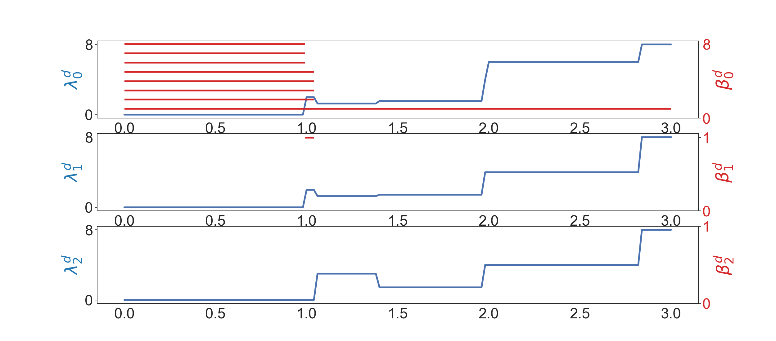
(h)

Figure 4:

Example 2.5.

(a) $d=0$

(b) $d=0.52$

(c) $d=1.00$

(d) $d=1.42$

(e) $d=1.74$

(f) $d=1.94$

(g) $d=2.00$

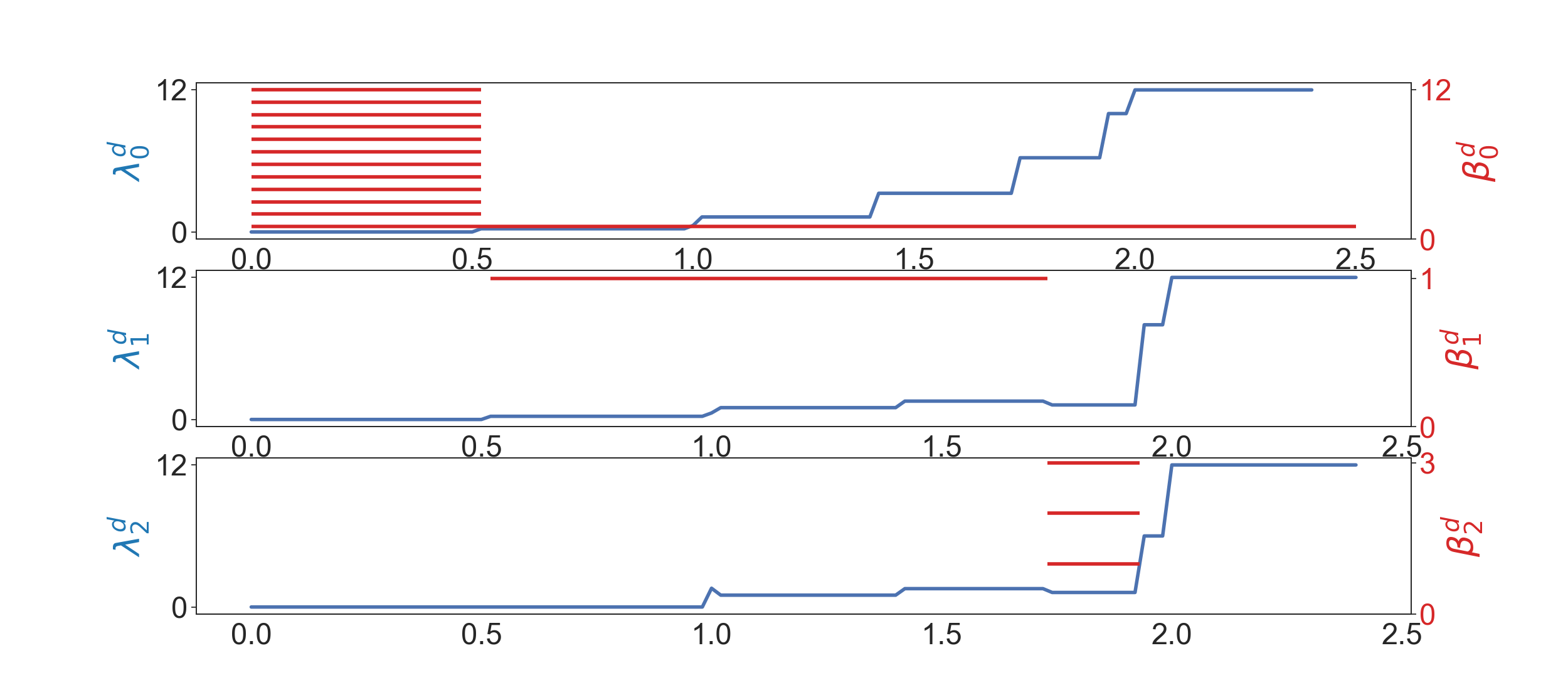
Figure 5:

We consider the Vietoris-Rips filtration of the 12 vertices of the regular 12-gon (Figure 5). We see that $\lambda^{d}_{2}$ goes up before any homology class is born, which means that $2$-simplices form but no $2$-dimensional holes are born yet. This phenomenon happens very often in many results of [102].

2.4 Matrix representations of a (persistent) Laplacian

Since any $C_{q}$ has a canonical orthonormal basis, the matrix representation of $\partial_{q}^{\ast}$ is the transpose of the matrix representation of $\partial_{q}$. For persistent Laplacians, the difficult part is the calculation of the up persistent Laplacian because we need to determine $C_{q+1}^{X,Y}$, which may not have a canonical orthonormal basis. We can obtain a basis of $C_{q+1}^{X,Y}$ by performing a column reduction for $\partial_{q+1}^{Y}$, or directly calculate the matrix representation of the up persistent Laplacian by Schur complement [73]. We give two calculation examples in Appendix.

2.5 Eigenvectors of a Laplacian

There are some results concerning the relation between the spectra of Laplacians and the shape of a simplicial complex [39, 53]. How do we interpret eigenvectors of a Laplacian? For an eigenvector of a $q$-th combinatorial Laplacian, we can look at the shape of $q$-simplices where the eigenvector has support (signs are arbitrary because they are affected by the fixed ordering of vertices). Empirical observations [60, 75, 104] suggest that: (a) harmonic eigenvectors (eigenvectors of zero eigenvalues) have support near $q$-dimensional “holes” (or vertices in a connected component when $q=0$); (b) nonharmonic eigenvectors (eigenvectors of nonzero eigenvalues) have support near “clusters” of $q$-simplices. As to a persistent Laplacian, very little is known about the geometrical/topological interpretation of eigenvalues and eigenvectors.

3 Generalizations of (persistent) Laplacians

From a theoretic point of view, it is natural to ask if a persistent Laplacian can be defined in other settings such that the persistent Hodge theorem still holds. From a practical point of view, generalizations of persistent Laplacians are motivated by the fact that simplicial complexes are not always adequate for the representation of data. One classic example is a scientist collaboration network. We may attempt to use a simplicial complex to represent collaborations among scientists, such that vertices are scientists and a simplex indicates that some scientists have coauthored at least one paper. Recall that in a simplicial complex any subset of a simplex is also a simplex, but a subset of coauthors may not necessarily coauthored one paper. Researchers have been searching for other structures in order to represent various types of data. Inspired by the success of topological data analysis, many attempts have been made to advance the theory of persistent homology and persistent Laplacians for complex data.

In the next few sections we will introduce structures such as cellular (co)sheaves, digraphs, and hyper(di)graphs, and then cover some recent advances in their homology and Laplacians. We will also discuss Dirac operators at the end of this section.

3.1 Differential graded inner product spaces

It has been noted early that persistent Laplacians can be defined analogously for differential graded inner product spaces and the persistent Hodge theorem can be proved in the same way. A differential graded inner product space $(V,d)$ is just a chain complex

whose chain groups are inner product spaces. When we say $(V,d^{V})$ is a subspace of $(W,d^{W})$, we mean that the inner space structure and boundary operator $d^{V}$ of $(V,d^{V})$ are inherited from $(W,d^{W})$. For a pair of differential graded inner product spaces $(V,d^{V})\subset(W,d^{W})$, the $q$-th persistent homology group is defined analogously by

$$\iota^{\bullet}(H_{q}(V))\cong\frac{\ker d_{q}^{V}}{\ker d_{q}^{V}\cap\operatorname{im}d_{q+1}^{W}}.$$

Observe that $\ker d_{q}^{V}\cap\operatorname{im}d_{q+1}^{W}=V_{q}\cap\operatorname{im}d_{q+1}^{W}$. The preimage of $V_{q}\cap\operatorname{im}d_{q+1}^{W}$ under $d_{q+1}^{W}$ is just $(d_{q+1}^{W})^{-1}(V_{q})=\{w\in W_{q+1}\mid d_{q+1}^{W}w\in V_{q}\}$. Hence, $\ker d_{q}^{V}\cap\operatorname{im}d_{q+1}^{W}$ is the image of $\pi d_{q+1}^{W}|_{(d_{q+1}^{W})^{-1}(V_{q})}:(d_{q+1}^{W})^{-1}(V_{q})\to V_{q}$, where $\pi=\iota^{{\dagger}}$, the projection map from $W$ to $V$. We denote $\pi d_{q+1}^{W}|_{(d_{q+1}^{W})^{-1}(V_{q})}$ by $d_{q+1}^{V,W}$, and $(d_{q+1}^{W})^{-1}(V_{q})$ by $\Theta_{q+1}^{V,W}$. These maps are shown in the following diagram

where hooked dashed arrows represent inclusion maps. If we define the $q$-th persistent Laplacian $\Delta_{q}^{V,W}:V_{q}\to V_{q}$ by

$$(d_{q}^{V})^{\ast}d_{q}^{V}+d_{q+1}^{V,W}(d_{q+1}^{V,W})^{\ast},$$

since $d_{q}^{V}d_{q+1}^{V,W}=0$, the persistent Hodge theorem

$$\ker\Delta_{q}^{V,W}\cong\frac{\ker d_{q}^{V}}{\ker d_{q}^{V}\cap\operatorname{im}d_{q+1}^{W}}$$

can be proved in the same way. Many generalizations of persistent Laplacians implicitly use this formulation. Liu et al. [66] first defined persistent Laplacians with differential graded inner product spaces and showed how to construct a persistent Laplacian for an inner product preserving chain map.

3.2 Persistent Laplacians for simplicial maps

The classical filtration of simplicial complexes only represents one type of shape evolution. We also need tools to study more general shape evolution, such as the sparsification of a simplicial complex. This requires us to consider general simplicial maps rather than inclusion maps. Gülen et al. [47] developed a theory of persistent Laplacians for a simplicial map. Suppose $f:X\to Y$ is a simplicial map,

where $f_{q}:C_{q}(X)\to C_{q}(Y)$ is induced by $f$. Different from the original $q$-th persistent Laplacian, we need to define two subspaces

$$C_{q+1}(Y)\supset C_{q+1}^{Y\leftarrow X}=\{c\in C_{q+1}(Y)\mid\partial_{q+1}^{Y}(c)\in f_{q}(\ker\partial_{q}^{X})\}$$

and

$$C_{q-1}(X)\supset C_{q-1}^{X\to Y}=\{c\in C_{q-1}^{X}\mid(\partial_{q}^{X})^{\ast}(c)\in(\ker f_{q})^{\bot}\}$$

and then use the restrictions of $\partial_{q+1}^{Y}$ and $(\partial_{q}^{X})^{\ast}$ to them to construct the $q$-th persistent Laplacian. The $q$-th persistent Laplacian for a simplicial map has a more symmetric expression, and the proof of the persistent Hodge theorem is more involved.

3.3 Weighted simplicial complexes

A simplicial complex whose simplices have weights is generally called a weighted simplicial complex. The weights can be geometrical, such as angles between simplices, volumes of simplices, or nongeometrical such as numbers of scientific papers coauthored by groups of people. Many theories and models involving weighted simplicial complexes exist (e.g., [4, 5, 27, 82, 94]). Here we focus on the theory of weighted simplicial complexes proposed by Robert J. MacG. Dawson [30] and later developed in [9, 10, 61, 85, 87, 107, 108]. A weighted simplicial complex is defined to be a simplicial complex where each simplex $\sigma$ has a weight $w(\sigma)$ valued in a commutative ring $R$, such that if $\sigma\leqslant\tau$, then $w(\tau)$ is divisible by $w(\sigma)$. The weighted chain complex of a weighted simplicial complex $X$ is defined as follows. Let $C_{q}(X,w)$ be the set of formal sums of $q$-simplices with coefficients in $R$ (if $w(\sigma)$ is zero then we do not include $\sigma$ in any formal sum). For $\sigma=[v_{a_{0}},\dots,v_{a_{q}}]$, we denote the face $[v_{a_{0}},\dots,\hat{v}_{a_{i}},\dots,v_{a_{q}}]$ by $d_{i}\sigma$. The weighted boundary operator $\partial$ is given by

$$\partial(\sigma)=\sum_{i=0}^{q}\frac{w(\sigma)}{w(d_{i}\sigma)}(-1)^{i}d_{i}\sigma.$$

As $w(\sigma)$ is divisible by $w(d_{i}\sigma)$, the weighted boundary operator is well-defined. We still have $\partial^{2}=0$, because for $0\leq i<j\leq q$,

$$\frac{w(\sigma)}{w(d_{i}\sigma)}\frac{w(d_{i}\sigma)}{w(d_{j-1}d_{i}\sigma)}=\frac{w(\sigma)}{w(d_{j}\sigma)}\frac{w(d_{j}\sigma)}{w(d_{i}d_{j}\sigma)}=\frac{w(\sigma)}{w(d_{i}d_{j}\sigma)}.$$

Therefore, weighted homology groups can be defined analogously. Wu et al. [107] pointed out that in the proof of $\partial^{2}=0$, what really matters is the quotient of weights. If we write $w(\tau)/w(\sigma)$ as $\phi(\sigma,\tau)$, then the equality

$$\frac{w(\sigma)}{w(d_{i}\sigma)}\frac{w(d_{i}\sigma)}{w(d_{j-1}d_{i}\sigma)}=\frac{w(\sigma)}{w(d_{j}\sigma)}\frac{w(d_{j}\sigma)}{w(d_{i}d_{j}\sigma)}$$

becomes

$$\phi(d_{i}\sigma,d_{j-1}d_{i}\sigma)\phi(\sigma,d_{i}\sigma)=\phi(d_{j}\sigma,d_{i}d_{j}\sigma)\phi(\sigma,d_{j}\sigma),$$

which means that any $\phi:X\times X\to R$ satisfying this equality induces a ($\phi$-weighted) boundary operator

$$\partial_{q}(\sigma)=\sum_{i=0}^{q}(-1)^{i}\phi(\sigma,d_{i}\sigma)d_{i}\sigma.$$

such that $\partial^{2}=0$. A simplicial complex paired with such a generalized weight function $\phi$ is called a $\phi$-weighted simplicial complex.

Example 3.1.

[107] A weighted polygon is a polygon with $\phi(\{v_{i},v_{j}\},v_{i})=\alpha_{i}\in\mathbb{Z}$ (Figure 6).

Figure 6: $X$

The matrix representation of $\partial_{1}$ is

$$\bordermatrix{~{}&v_{0}v_{1}&v_{0}v_{4}&v_{1}v_{2}&v_{2}v_{3}&v_{3}v_{4}\cr v_{0}&-\alpha_{0}&-\alpha_{0}&0&0&0\cr v_{1}&\alpha_{1}&0&-\alpha_{1}&0&0\cr v_{2}&0&0&\alpha_{2}&-\alpha_{2}&0\cr v_{3}&0&0&0&\alpha_{3}&-\alpha_{3}\cr v_{4}&0&\alpha_{4}&0&0&\alpha_{4}\cr}$$

and the resulting weighted $H_{0}$ is dependent on $\alpha_{i}$. The weighted homology of weighted polygons might be useful for studying ring structures in biomolecules.

We have emphasized that a point cloud can be studied by building a filtration of simplicial complexes. If we want to distinguish some points from other points, we can assign weights and building a filtration of weighted simplicial complexes [87]. We may also consider weighted versions of (persistent) Laplacians [107].

Example 3.2.

Suppose each point $v$ in a point cloud has weight $w(v)$. We can associate any simplex $\{v_{a_{0}},\dots,v_{a_{q}}\}$ the product weight [87]

$$\prod_{i=0}^{q}w(v_{a_{i}}).$$

Since the weighted boundary map can be given by

$$\partial(\sigma)=\sum_{i=0}^{q}w(v_{a_{i}})(-1)^{i}d_{i}\sigma.$$

We can just define the $q$-th chain group as the space generated by $q$-simplices without worrying if any of their weights is zero or not.

Example 3.3.

Suppose a poind cloud contains two types of points $A$ and $B$. We can assign weights $0,1$ to $A,B$, and compute weighted homology and Laplacians using product weighting. At least when a point cloud is simple, weighted combinatorial Laplacians can be used to differentiate among different patterns of distribution of $A$ and $B$. For a point cloud of four points $\{(0,0),(1,0),(1,1),(0,1)\}$ there are five configurations (shown in Figure 7) that include at least one point whose weight is 1. Results of weighted Laplacians are shown in Figure 8.

(a)

(b)

(c)

(d)

(e)

Figure 7:

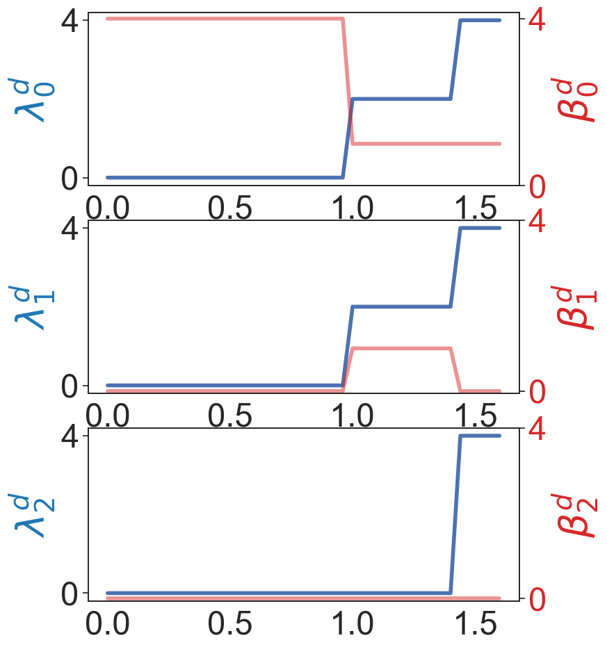
(a) $BBBB$

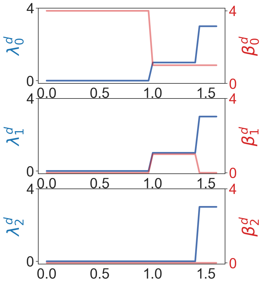
(b) $ABBB$

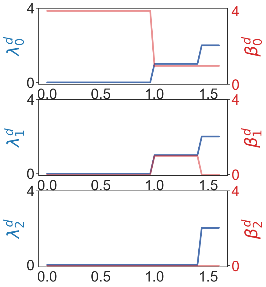
(c) $AABB$

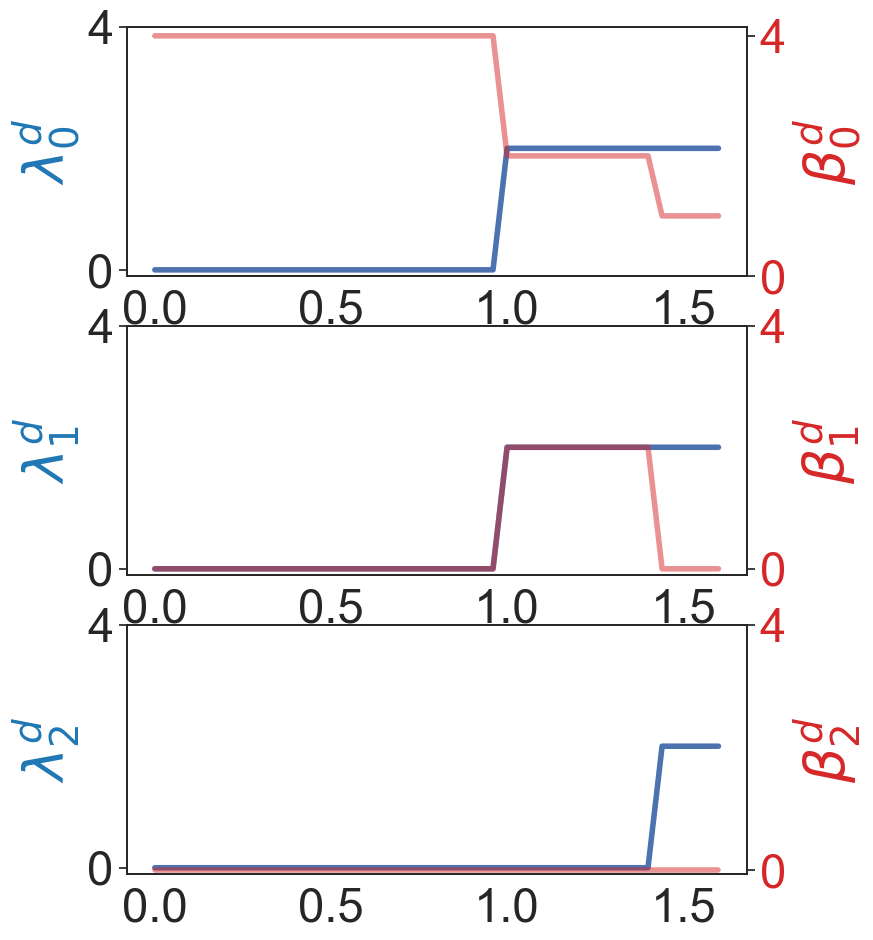
(d) $ABAB$

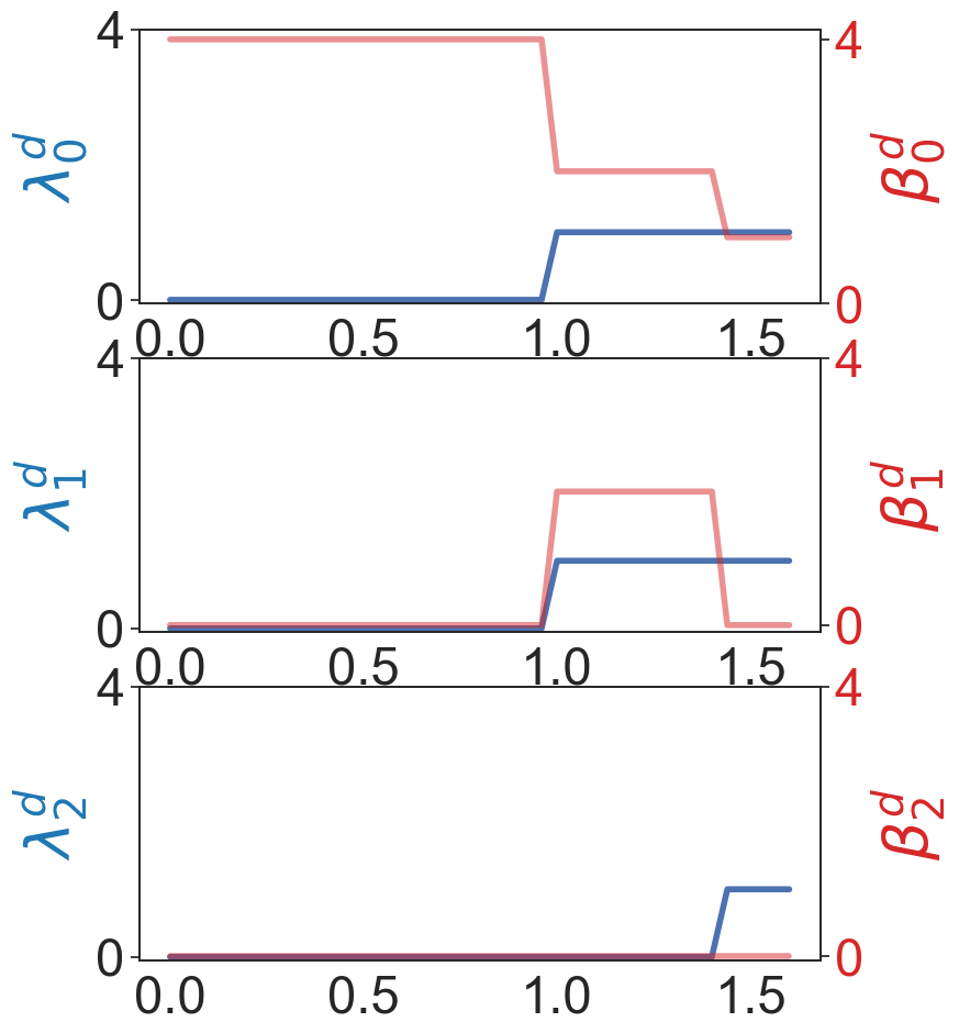
(e) $AAAB$

Figure 8: $\lambda^{d}_{q}$ is the minimal nonzero eigenvalue of the $q$-th weighted combinatorial Laplacian for $X_{d}$ in a Rips filtration. $\beta^{d}_{q}$ is the $q$-th Betti number of $X_{d}$.

3.4 Cellular (co)sheaves

Persistent homology neglects vital physical, chemical, and biological interactions in its direct applications to molecular science. To address this drawback, bio-inspired element-specific persistent homology was proposed. The idea is to split the input point cloud into multiple subgroups so as to better characterize physical and chemical interactions [11, 12]. Another more elegant approach is persistent cohomology, which allows the incorporation of non-geometrical information into the topological invariants [13]. Sheaf Laplacians and persistent sheaf Laplacians [106] offer an alternative approach to embed non-geometric information into topological invariants.

In a $\phi$-weighted simplicial complex, we can imagine that on each simplex lives a copy of $R$ and $\phi(\tau,\sigma)$ is a scalar multiplication from the copy on $\tau$ to the copy on $\sigma$ [50]. If we associate each simplex with a vector space and designate a linear morphism for every face relation, we will get a cellular (co)sheaf. The theory of cellular (co)sheaves was first introduced in [96] and later attracted attention for its application potential (e.g., [28, 49, 91, 92, 111]). Like a weighted simplicial complex, a cellular (co)sheaf is a candidate for modeling complex objects such as molecules.

A cellular cosheaf $\mathscr{F}$ is a simplicial complex $X$ with additional data. Each simplex $\sigma$ is assigned a vector space $\mathscr{F}(\sigma)$ (or denoted by $\mathscr{F}_{\sigma}$), referred to as the stalk over $\sigma$, and for any face relation $\sigma\leqslant\tau$, there is an extension map $\mathscr{F}(\sigma\leqslant\tau):\mathscr{F}(\tau)\to\mathscr{F}(\sigma)$ (or denoted by $\mathscr{F}_{\sigma\leqslant\tau}$). The $q$-th chain group of a cellular cosheaf is the direct sum of stalks over $q$-simplices and the boundary map $\partial$ is given by

$$\partial_{q}|_{\mathscr{F}(\sigma)}=\sum_{i}(-1)^{i}\mathscr{F}(d_{i}\sigma\leqslant\sigma).$$

The square of this boundary map is 0, if for any face relation $\rho\leqslant\sigma\leqslant\tau$ we have

$$\mathscr{F}(\rho\leqslant\tau)=\mathscr{F}(\rho\leqslant\sigma)\circ\mathscr{F}(\sigma\leqslant\tau).$$

A dual concept is a cellular sheaf. For a cellular sheaf $\mathscr{F}$, $\mathscr{F}(\sigma\leqslant\tau)$ is a map from $\mathscr{F}(\sigma)$ to $\mathscr{F}(\tau)$ (called a restriction map). A sheaf cochain complex can be defined analogously. If stalks are inner product spaces, one can equip inner product structures for (co)chain groups. Applying the construction of combinatorial Laplacians to a cosheaf chain complex or sheaf cochain complex, we get (co)sheaf Laplacians [50]. It is noted that many sheaves over a digraph only have trivial 0-dimensional cohomology groups [48], but we can still extract some information from sheaf Laplacians.

Example 3.4.

Suppose there is a sheaf $\mathscr{F}$ over the simplicial complex $\{0,1,2,01,02,12\}$, then the sheaf coboundary map $\delta^{0}$ is represented by the block matrix

$$\bordermatrix{~{}&\mathscr{F}_{0}&\mathscr{F}_{1}&\mathscr{F}_{2}\cr\mathscr{F}_{01}&-\mathscr{F}_{0\leqslant 01}&\mathscr{F}_{1\leqslant 01}&0\cr\mathscr{F}_{02}&-\mathscr{F}_{0\leqslant 02}&0&\mathscr{F}_{2\leqslant 02}\cr\mathscr{F}_{12}&0&-\mathscr{F}_{1\leqslant 12}&\mathscr{F}_{2\leqslant 12}\cr}.$$

Suppose all stalks are inner product spaces and they are orthogonal to each other, the $0$-th sheaf Laplacian ${\delta^{0}}^{\ast}\delta^{0}$ is represented by the block matrix

$$\bordermatrix{~{}&\mathscr{F}_{0}&\mathscr{F}_{1}&\mathscr{F}_{2}\cr\mathscr{F}_{0}&\mathscr{F}_{0\leqslant 01}^{\ast}\mathscr{F}_{0\leqslant 01}+\mathscr{F}_{0\leqslant 02}^{\ast}\mathscr{F}_{0\leqslant 02}&-\mathscr{F}_{0\leqslant 01}^{\ast}\mathscr{F}_{1\leqslant 01}&-\mathscr{F}_{0\leqslant 02}^{\ast}\mathscr{F}_{2\leqslant 02}\cr\mathscr{F}_{1}&-\mathscr{F}_{1\leqslant 01}^{\ast}\mathscr{F}_{0\leqslant 01}&\mathscr{F}_{1\leqslant 01}^{\ast}\mathscr{F}_{1\leqslant 01}+\mathscr{F}_{1\leqslant 12}^{\ast}\mathscr{F}_{1\leqslant 12}&-\mathscr{F}_{1\leqslant 12}^{\ast}\mathscr{F}_{2\leqslant 12}\cr\mathscr{F}_{2}&-\mathscr{F}_{2\leqslant 02}^{\ast}\mathscr{F}_{0\leqslant 02}&-\mathscr{F}_{2\leqslant 12}^{\ast}\mathscr{F}_{1\leqslant 12}&\mathscr{F}_{2\leqslant 02}^{\ast}\mathscr{F}_{2\leqslant 02}+\mathscr{F}_{2\leqslant 12}^{\ast}\mathscr{F}_{2\leqslant 12}\cr}.$$

Persistent (co)sheaf (co)homology is known to experts [90, 110] and a systematical treatment can be found in [93]. One type of filtration of sheaves is as follows. We may say $\mathscr{F}$ over $X$ is a “subsheaf” of $\mathscr{G}$ over $Y$ if $X\subset Y$ and stalks and restriction maps of $\mathscr{F}$ are the same as those of $\mathscr{G}$. To define the $q$-th persistent sheaf Laplacian [106] for $\mathscr{F}\subset\mathscr{G}$, we can first endow chain groups with inner product structures and dualize everything to make $\mathscr{F}$ and $\mathscr{G}$ cosheaves, such that there is an inclusion chain map between their cosheaf chain complexes. Then we can define the $q$-th persistent sheaf Laplacian as the $q$-th persistent Laplacian of cosheaf chain complexes.

3.5 Path homology, flag homology, and digraphs

The motivation behind path homology is to construct a homology theory of digraphs such that directional information of edges is encoded and higher dimensional homology groups are non-trivial. Path homology was proposed by Grigor’yan, Lin, Muranov and Yau [42] and developed in [43, 44, 45, 46, 64]. A summary of recent advances in path homology of digraphs can be found in [41]. Recall that a digraph (without self-loops) is a pair $G=(V,E)$ where $E$ is a set of ordered pairs of vertices. An allowed $q$-path is an ordered finite sequence of vertices $\{x_{0},\dots,x_{q}\}$ such that $(x_{i},x_{i+1})\in E$ for all $0\leq i\leq q-1$. If we take the space generated by allowed $p$-paths (denoted by $\mathcal{A}_{q}$) as the $q$-th chain group, and define the boundary map $\partial_{q}$ by

$$\partial_{q}\{x_{0},\dots,x_{q}\}=\sum_{i=0}^{q}(-1)^{i}\{x_{0},\dots,\hat{x}_{i},\dots,x_{q}\}$$

then formally we can show that $\partial^{2}=0$. But the problem is that, $\partial_{q}\{x_{0},\dots,x_{q}\}$ may include paths that are not allowed (indeed $\partial^{2}=0$ only makes sense when $\partial_{q}$ is viewed as a map in larger spaces). One way to make $\partial_{q}:\mathcal{A}_{q}\to\mathcal{A}_{q-1}$ well-defined is to restrict $\partial_{q}$ to the subspace $\mathcal{A}_{q}\cap\partial_{q}^{-1}\mathcal{A}_{q-1}$. We have to verify that $\partial_{q}(\mathcal{A}_{q}\cap\partial_{q}^{-1}\mathcal{A}_{q-1})\subset\mathcal{A}_{q-1}\cap\partial_{q-1}^{-1}\mathcal{A}_{q-2}$. $\partial_{q}(\mathcal{A}_{q}\cap\partial_{q}^{-1}\mathcal{A}_{q-1})\subset\mathcal{A}_{q-1}\cap$ is true by definition, and $\partial_{q}(\mathcal{A}_{q}\cap\partial_{q}^{-1}\mathcal{A}_{q-1})\subset\partial_{q-1}^{-1}\mathcal{A}_{q-2}$ is true since $\partial^{2}=0$. Therefore, we have the chain complex

and the definition of a path homology group is straightforward. The $q$-th chain group $\mathcal{A}_{q}\cap\partial_{q}^{-1}\mathcal{A}_{q-1}$ is called the space of $\partial$-invariant $q$-paths on $G$, denoted by $\Omega_{q}$.

As to the geometrical interpretation of path homology, we only know for sure that non-reduced $H_{0}$ is the number of connected components of the underlying undirected graph. It is not easy to relate higher dimensional path homology groups to features of a digraph. Chowdhury et al. [21] obtained some characterizations of path homologies of certain families of small digraphs. Since directional information of edges is encoded in path homology, path homology can be used to distinguish network motifs [22] and isomers in molecular and materials sciences [16]. We can also quantify the significance of a node in a network by observing the changes of path homology when the node is removed [16].

Since $\Omega_{q}$ inherits the inner product structure from $\mathcal{A}_{q}$, the so-called path Laplacians can be defined. We can use path Laplacians [40, 41, 101] to distinguish among digraphs that path homology cannot. For example, according to [42, Theorem 5.4], the following two digraphs $G_{L}$ and $G_{R}$ (see Figure 9) have the same path homology. But the spectrum of the $0$-th path Laplacian of $G_{L}$ is $\{0,3,3\}$ and that of $G_{R}$ is $\{0,2,4,4\}$. We also note that another type of path Laplacians were proposed by Estrada [36] and was generalized and applied in molecular biology in [68].

(a) $G_{L}$

(b) $G_{R}$

Figure 9: Two distinct digraphs.

Persistent path homology was proposed by Chowdhury and Mémoli [22] to study a digraph where each edge $e$ has a weight $w(e)$. A filtration of digraphs $\{G_{d}\}$ is constructed such that $e\in G_{d}$ if and only if $w(e)\leq d$. Wang and Wei [101] introduced persistent path Laplacians and demonstrated that persistent path Laplacians can be applied to study molecules, where much information can be encoded in a digraph.

Flag complexes, also known as clique complexes, arise naturally in many situations [70]. Jones and Wei introduced persistent directed flag Laplacians as a distinct way of analyzing flag complexes [57]. Persistent directed flag Laplacians were applied to protein-ligand binding data.

Example 3.5.

For a weighted digraph, we can build a filtration $\{G_{d}\}$ such that $e\in G_{d}$ iff $w(e)\leq d$. Two weighted graphs whose path Betti numbers are the same for every $G_{d}$ may have different path Laplacians.

(a)

(b)

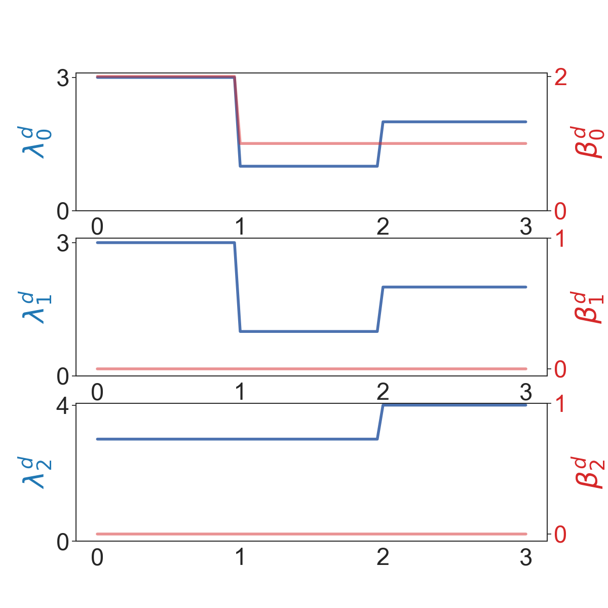
(c) Results of the left graph

(d) Results of the right graph

Figure 10: In (a) and (b), numbers on edges are weights. In (c) and (d), the $x$ axis represents the weight. As usual, $\lambda$ and $\beta$ represent the minimal eigenvalues and Betti numbers.

3.6 Hypergraphs and hyperdigraphs

A hypergraph $H$ is a pair $(V,E)$ where $E$ is a subset of the power set of $V$. An element $e\in E$ that consists of $q+1$ elements is called a $q$-hyperedge. To define a chain complex for hypergraphs, the problem here is identical to what we encounter in path homology. If we define the $q$-th chain group to be the vector space generated by $q$-hyperedges, the boundary map is not well-defined. One solution is to consider the associated simplicial complex (simplicial closure) of a hypergraph [81], i.e., the minimal simplicial complex that contains a hypergraph. Another solution inspired by the path homology is the embedded homology [7]. If we look at the chain complex of the associated simplicial complex, each simplicial chain group $C_{q}$ contains $D_{q}$, the vector space generated by $q$-hyperedges. We only need to restrict the domain of the simplicial boundary operator to

$$\text{Inf}_{q}=D_{q}\cap\partial_{q}^{-1}(D_{q}),$$

and then the boundary operator is well-defined.

Figure 11: $C_{q}$ is the $q$-th chain group of the associated simplicial complex of $H$, and $D_{q}$ is the vector space generated by $q$-hyperedges.

A hyperdigraph is a hypergraph where each hyperedge is ordered, the embedded homology of which can be defined similarly [15]. Persistent homology of hypergraphs and hyperdigraphs are studied in [7, 86, 88]. Persistent hypergraph Laplacians were proposed by Liu et al. [69] and persistent hyperdigraph Laplacians [15] were introduced by Chen et al. Other approaches regarding the homology and Laplacians of hypergraph includes [23, 35, 54, 58, 77, 78].

3.7 Persistent Dirac operators

Besides Laplacians, Dirac operators on chain complexes have also been studied [2, 6, 97, 103]. Given a chain complex $(V,d)$

where each chain group $V_{q}$ is a finite dimensional inner product space, the $q$-th Dirac operator $D_{q}$ is represented by the block matrix

$$\bordermatrix{~{}&V_{0}&V_{1}&V_{2}&\cdots&V_{q}&V_{q+1}\cr V_{0}&0&[d_{1}]&0&\cdots&0&0\cr V_{1}&[d_{1}^{\ast}]&0&[d_{2}]&\cdots&0&0\cr V_{2}&0&[d_{2}^{\ast}]&0&\cdots&0&0\cr\vdots&\vdots&\vdots&\vdots&\ddots&\vdots&\vdots\cr V_{q}&0&0&0&\cdots&0&[d_{q+1}]\cr V_{q+1}&0&0&0&\cdots&[d_{q+1}^{\ast}]&0\cr}$$

where $[]$ denotes a matrix representation of a linear morphism. Dirac operators are closely related to combinatorial Laplacians. If we think of all combinatorial Laplacians as a single operator $dd^{\ast}+d^{\ast}d=(d+d^{\ast})^{2}$ on $V$, then the $q$-th Dirac operator is the restriction of the square root $d+d^{\ast}$ on $V_{0}\oplus\cdots\oplus V_{q+1}$. We can also see this by direct computation. The square of $D_{q}$ is

$$\bordermatrix{~{}&V_{0}&V_{1}&V_{2}&\cdots&V_{q}&V_{q+1}\cr V_{0}&[\Delta_{0}]&0&0&\cdots&0&0\cr V_{1}&0&[\Delta_{1}]&0&\cdots&0&0\cr V_{2}&0&0&[\Delta_{2}]&\cdots&0&0\cr\vdots&\vdots&\vdots&\vdots&\ddots&\vdots&\vdots\cr V_{q}&0&0&0&\cdots&[\Delta_{q}]&0\cr V_{q+1}&0&0&0&\cdots&0&[\Delta_{q+1,-}]\cr}$$

where $\Delta_{q}$ is the $q$-th combinatorial Laplacian. Therefore, the square of any eigenvalue $\lambda$ of a Dirac operator must be an eigenvalue of a combinatorial Laplacian.

Recall that to define persistent Laplacians, we construct an auxiliary subspace $C_{q+1}^{X,Y}$ of $C_{q+1}(Y)$ and a map $\partial_{q+1}^{X,Y}:C_{q+1}^{X,Y}\to C_{q}(X)$. Since $C_{q}(X)$ is actually a subspace of $C_{q}^{X,Y}$, all $C_{q}^{X,Y}$ and $\partial_{q}^{X,Y}$ constitute an auxiliary chain complex

The $q$-th persistent Dirac operator of simplicial complexes $X\subset Y$ is just the $q$-th Dirac operator on this auxiliary complex. In general, Dirac matrices involved coupled dimensions, which may be more difficult to compute. The square of a persistent Dirac operator is not necessarily a block matrix consisting of persistent Laplacians. Suwayyid and Wei considered the generalization of persistent Dirac operators to other settings such as path complexes and hypergraphs [97].

3.8 Mayer homology

In algebraic topology, the square of the boundary operator $d$ of a chain complex must be zero. However, this constraint can be relaxed in the so called Mayer homology theory using the $N$-chain complex [72]. An $N$-chain complex is a sequence of abelian groups and group morphisms $(V,d)$ where $d^{N}=0$. A simplicial complex can actually give rise to an $N$-chain complex. Recall that in a simplicial chain complex the boundary operator is given by

$$\partial[v_{a_{0}},\dots,v_{a_{q}}]=\sum_{i}(-1)^{i}[v_{a_{0}},\dots,\hat{v}_{a_{i}},\dots,v_{a_{q}}].$$

For a prime number $N$, let $\xi=e^{2\pi\sqrt{-1}/N}$, we can define a generalized boundary operator $d$ by

$$d[v_{a_{0}},\dots,v_{a_{q}}]=\sum_{i}\xi^{i}[v_{a_{0}},\dots,\hat{v}_{a_{i}},\dots,v_{a_{q}}]$$

and prove that $d^{N}=0$. Even though $N$-chain complex is not a chain complex in general, observe that for any positive integer $n<N$

resembles a part of chain complex. We can define the Mayer homology group $H_{q,n}(X)=\ker d^{n}/\operatorname{im}d^{N-n}$ [72] and Mayer Laplacians (which can be thought of as $(d^{n}+(d^{N-n})^{\ast})((d^{n})^{\ast}+d^{N-n})$) analogously [95]. When $N=2$, a $N$-chain complex reduces to a chain complex and a Mayer homology group reduces to a normal homology group. Shen et al. [95] also introduced persistent Mayer homology and persistent Mayer Laplacians on $N$-chain complexes. Suppose $X\subset Y$, then we have the following commutative diagram

and persistent Laplacians can be defined analogously. Compared to simplicial homology, Mayer homology and Mayer Laplacians provide much more features since we can vary parameters $N$ and $n$. Besides, Mayer homology and Mayer Laplacians concerns general relations between different dimensions.

4 Concluding remarks

The development of persistent topological Laplacians (PTLs) was in a large part inspired by persistent homology’s limitations in modeling complex biomolecular data [20, 100]. The techniques we reviewed in this survey transform a point cloud or a network to a set of algebraic features that encode not only topological invariants but also geometrical information. Some specific technique, namely the persistent sheaf Laplacian approach, allows us to embed physical law or heterogeneous information into algebraic invariants. PTLs offer new ways of comparing different structures, especially when they are highly related, such as different configurations of a single molecule. PTLs can be viewed as dimension reduction techniques that map data in high dimensions to a low dimensional space. The resulting low dimensional representations can be further used in supervised/unsupervised machine learning to reveal hidden information. In general, for a given data, PTLs provide unique representations that cannot be obtained by other alternative means in mathematics and science. The superiority of persistent Laplacians over persistent homology has been demonstrated in recent applications to 34 datasets in protein engineering [83] and its power has been verified in the forecasting of emerging dominant viral variants [17].

The field of PTLs is dynamic and rapidly evolving. The future development of PTLs is widely open, and we envision the exploration of the following topics.

(1) Given a point cloud or a network, the diversity of PTLs makes it challenging to fully understand the relationship between the geometry/topology of the data and spectra of PTLs. The understanding of this relationship is crucial for the application of PTLs to real world problems.

(2) To a certain extent, the success of persistent homology can be attributed to its integration with machine learning, particularly with the introduction of topological deep learning [11]. Similarly, the development of efficient PTL representations and vectorizations of data for machine learning, including deep learning, is also an important topic. The featurization of Laplacians typically requires domain knowledge and experience. Since self learning representations of persistent diagrams have been proposed [52], we wonder if self learning representations of (persistent) Laplacians are possible. It is also interesting to featurize the eigenvectors of Laplacians. For example, the eigenvectors of persistent flag Laplacians were found to have better descriptive power than eigenvalues [57].

(3) Despite efforts in software development [73, 102], the computation of PTLs remains slow, particularly for problems involving large datasets. Since the primary value of TDA lies in its ability to tackle challenges in data science, one of the most pressing needs will be the development of efficient and robust PTL software packages to solve real-world problems. As the finite field formulation of persistent homology is essential for fast algorithms in TDA. The development of finite field PTLs will be extremely valuable for the implementation of PTLs in data science.

(4) PTLs have been formulated on a variety of mathematical objects, including simplicial complexes, flag complexes, path complexes, cellular sheaf, digraphs, hypergraphs, and hyperdigraph. We can also extend PTLs to settings such as the Hoschild complex, Khovanov homology [59], multiparameter persistent homology [51], and interaction homotopy and interaction homology [65].

(5) As mentioned in [97], a few more persistent Dirac operators can be formulated for flag complexes, digraphs, hyperdigraphs, etc. It may be possible that a persistent sheaf Dirac operator can be devised to distinguish certain geometric shapes.

(6) The PTLs on manifolds, such as the evolutionary de Rham-Hodge theory, pose implementation challenges compared to their discrete counterparts on point clouds [89]. However, from a theorectical point of view, it will be interesting to generalize various PTLs on point clouds to the manifold setting.

(7) Most recently, persistent Mayer homology and persistent Mayer Laplacians have been introduced on $N$-chain complexes [95]. These formulations encompass persistent homology and persistent Laplacians as special cases. The potential for future developments in these subjects is widely open.

(8) Finally, ChatGPT ushers in a new era of artificial intelligence (AI), offering widespread opportunities in all disciplines. ChatGPT and other chatbots effectively transform pure mathematical theories into practical computational tools, including PTLs [67]. This AI approach will have a growing impact on computational and applied topology.

5 Appendix

5.1 The calculation of a persistent Laplacian

Example 5.1.

(a)

(b)

Figure 12: $X=\{0,1,2,3,01,12,02\}$ and $Y=\{0,1,2,3,01,12,23,03,02,012,023\}$.

When $C_{q+1}^{X,Y}$ is generated by some $(q+1)$-simplices in $Y$, the calculation of $\partial_{q}^{X,Y}$ is relatively easy. For $X$ and $Y$ shown in Figure 12, the matrix representation of $\partial_{2}^{Y}$ is

$$\bordermatrix{~{}&012&023\cr 01&1&0\cr 12&1&0\cr 02&-1&1\cr 23&0&1\cr 03&0&-1\cr},$$

so $C_{2}^{X,Y}$ is generated by $012$, then the matrix representation of $\partial_{2}^{X,Y}$ is

$$\bordermatrix{~{}&012\cr 01&1\cr 12&1\cr 02&-1\cr}.$$

Example 5.2.

We compute the persistent Laplacian $\Delta_{1}^{X,Y}$ for $X$ and $Y$ shown in Figure 13.

(a)

(b)

Figure 13: $X=\{0,1,2,3,01,12,23,03\}$ and $Y=\{0,1,2,3,01,12,23,03,02,012,023\}$.

The matrix representation of $\partial_{2}^{Y}$ is

$$\bordermatrix{~{}&012&023\cr 01&1&0\cr 12&1&0\cr 23&0&1\cr 03&0&-1\cr 02&-1&1\cr}.$$

Our goal is to make the submatrix

$$\bordermatrix{~{}&012&023\cr 02&-1&1\cr}$$

in column echelon form. We apply one column reduction and get

$$\bordermatrix{~{}&012&023+012\cr 01&1&1\cr 12&1&1\cr 23&0&1\cr 03&0&-1\cr 02&-1&0\cr}.$$

Therefore, $C_{2}^{X,Y}=\text{span}(023+012)$ and one matrix representation of $\partial_{2}^{X,Y}$ is

References

- [1] H. Adams, T. Emerson, M. Kirby, R. Neville, C. Peterson, P. Shipman, S. Chepushtanova, E. Hanson, F. Motta, and L. Ziegelmeier. Persistence images: A stable vector representation of persistent homology. Journal of Machine Learning Research, 18, 2017.
- [2] B. Ameneyro, V. Maroulas, and G. Siopsis. Quantum persistent homology. arXiv preprint arXiv:2202.12965, 2022.
- [3] G. Ausiello and L. Laura. Directed hypergraphs: Introduction and fundamental algorithms—a survey. Theoretical Computer Science, 658:293–306, 2017.
- [4] F. Baccini, F. Geraci, and G. Bianconi. Weighted simplicial complexes and their representation power of higher-order network data and topology. Physical Review E, 106(3):034319, 2022.
- [5] C. Battiloro, S. Sardellitti, S. Barbarossa, and P. Di Lorenzo. Topological signal processing over weighted simplicial complexes. arXiv preprint arXiv:2302.08561, 2023.
- [6] G. Bianconi. The topological dirac equation of networks and simplicial complexes. Journal of Physics: Complexity, 2(3):035022, 2021.
- [7] S. Bressan, J. Li, S. Ren, and J. Wu. The embedded homology of hypergraphs and applications. Asian Journal of Mathematics, 23(3):479–500, 2019.
- [8] P. Bubenik et al. Statistical topological data analysis using persistence landscapes. J. Mach. Learn. Res., 16(1):77–102, 2015.
- [9] A. Bura, Q. He, and C. Reidys. Weighted homology of bi-structures over certain discrete valuation rings. Mathematics, 9(7):744, 2021.
- [10] A. C. Bura, N. S. Dutta, T. J. Li, and C. M. Reidys. A computational framework for weighted simplicial homology. arXiv preprint arXiv:2206.04612, 2022.
- [11] Z. Cang and G.-W. Wei. Topologynet: Topology based deep convolutional and multi-task neural networks for biomolecular property predictions. PLoS computational biology, 13(7):e1005690, 2017.
- [12] Z. Cang and G.-W. Wei. Integration of element specific persistent homology and machine learning for protein-ligand binding affinity prediction. International journal for numerical methods in biomedical engineering, 34(2):e2914, 2018.
- [13] Z. Cang and G.-W. Wei. Persistent cohomology for data with multicomponent heterogeneous information. SIAM Journal on Mathematics of Data Science, 2(2):396–418, 2020.
- [14] L. Caputi and H. Riihimäki. Hochschild homology, and a persistent approach via connectivity digraphs. Journal of Applied and Computational Topology, pages 1–50, 2023.
- [15] D. Chen, J. Liu, J. Wu, and G.-W. Wei. Persistent hyperdigraph homology and persistent hyperdigraph laplacians. Foundations of Data Science, 2023.
- [16] D. Chen, J. Liu, J. Wu, G.-W. Wei, F. Pan, and S.-T. Yau. Path topology in molecular and materials sciences. The Journal of Physical Chemistry Letters, 14(4):954–964, 2023.
- [17] J. Chen, Y. Qiu, R. Wang, and G.-W. Wei. Persistent laplacian projected omicron ba. 4 and ba. 5 to become new dominating variants. Computers in Biology and Medicine, 151:106262, 2022.
- [18] J. Chen, R. Wang, M. Wang, and G.-W. Wei. Mutations strengthened sars-cov-2 infectivity. Journal of molecular biology, 432(19):5212–5226, 2020.
- [19] J. Chen, D. R. Woldring, F. Huang, X. Huang, and G.-W. Wei. Topological deep learning based deep mutational scanning. Computers in Biology and Medicine, 164:107258, 2023.
- [20] J. Chen, R. Zhao, Y. Tong, and G.-W. Wei. Evolutionary de rham-hodge method. arXiv preprint arXiv:1912.12388, 2019.
- [21] S. Chowdhury, S. Huntsman, and M. Yutin. Path homologies of motifs and temporal network representations. Applied Network Science, 7(1):4, 2022.
- [22] S. Chowdhury and F. Mémoli. Persistent path homology of directed networks. In Proceedings of the Twenty-Ninth Annual ACM-SIAM Symposium on Discrete Algorithms, pages 1152–1169. SIAM, 2018.
- [23] F. R. Chung. The laplacian of a hypergraph. In Expanding graphs, pages 21–36, 1992.
- [24] F. R. Chung. Spectral graph theory, volume 92. American Mathematical Soc., 1997.
- [25] J. R. Clough, N. Byrne, I. Oksuz, V. A. Zimmer, J. A. Schnabel, and A. P. King. A topological loss function for deep-learning based image segmentation using persistent homology. IEEE transactions on pattern analysis and machine intelligence, 44(12):8766–8778, 2020.
- [26] S. Cottrell, R. Wang, and G. Wei. Plpca: Persistent laplacian enhanced-pca for microarray data analysis. J. Chem. Inf. Model., page https://doi.org/10.1021/acs.jcim.3c01023, 2023.
- [27] O. T. Courtney and G. Bianconi. Weighted growing simplicial complexes. Physical Review E, 95(6):062301, 2017.
- [28] J. Curry. Sheaves, cosheaves and applications. PhD thesis, University of Pennsylvania, 2014.
- [29] Y. Dabaghian, F. Mémoli, L. Frank, and G. Carlsson. A topological paradigm for hippocampal spatial map formation using persistent homology. 2012.
- [30] R. J. M. Dawson. Homology of weighted simplicial complexes. Cahiers de Topologie et Géométrie Différentielle Catégoriques, 31(3):229–243, 1990.
- [31] M. Desbrun, E. Kanso, and Y. Tong. Discrete differential forms for computational modeling. In ACM SIGGRAPH 2006 Courses, pages 39–54. 2006.
- [32] H. Du, G.-W. Wei, and T. Hou. Multiscale topology in interactomic network: From transcriptome to antiaddiction drug repurposing. arXiv preprint arXiv:2312.01272, 2023.
- [33] B. Eckmann. Harmonische funktionen und randwertaufgaben in einem komplex. Commentarii Mathematici Helvetici, 17(1):240–255, 1944.
- [34] H. Edelsbrunner, J. Harer, et al. Persistent homology-a survey. Contemporary mathematics, 453(26):257–282, 2008.
- [35] E. Emtander. Betti numbers of hypergraphs. Communications in algebra, 37(5):1545–1571, 2009.
- [36] E. Estrada. Path laplacian matrices: introduction and application to the analysis of consensus in networks. Linear algebra and its applications, 436(9):3373–3391, 2012.
- [37] M. Fiedler. Algebraic connectivity of graphs. Czechoslovak mathematical journal, 23(2):298–305, 1973.
- [38] R. Ghrist. Barcodes: the persistent topology of data. Bulletin of the American Mathematical Society, 45(1):61–75, 2008.
- [39] T. E. Goldberg. Combinatorial laplacians of simplicial complexes. Senior Thesis, Bard College, 2002.
- [40] A. Gomes and D. Miranda. Path cohomology of locally finite digraphs, hodge’s theorem and the -lazy random walk. arXiv preprint arXiv:1906.04781, 2019.
- [41] A. Grigor’yan. Advances in path homology theory of digraphs. 2022.
- [42] A. Grigor’yan, Y. Lin, Y. Muranov, and S.-T. Yau. Homologies of path complexes and digraphs. arXiv preprint arXiv:1207.2834, 2012.
- [43] A. Grigor’yan, Y. Lin, Y. Muranov, and S.-T. Yau. Homotopy theory for digraphs. Pure and Applied Mathematics Quarterly, 10(4):619–674, 2014.
- [44] A. Grigor’yan, Y. Lin, Y. Muranov, and S.-T. Yau. Cohomology of digraphs and (undirected) graphs. Asian Journal of Mathematics, 19(5):887–932, 2015.
- [45] A. Grigor’yan, Y. Lin, Y. V. Muranov, and S.-T. Yau. Path complexes and their homologies. Journal of Mathematical Sciences, 248:564–599, 2020.
- [46] A. Grigor’yan, Y. Muranov, and S.-T. Yau. Homologies of digraphs and künneth formulas. Communications in Analysis and Geometry, 25(5):969–1018, 2017.
- [47] A. B. Gülen, F. Mémoli, Z. Wan, and Y. Wang. A generalization of the persistent laplacian to simplicial maps. arXiv preprint arXiv:2302.03771, 2023.
- [48] J. Hansen. A gentle introduction to sheaves on graphs.
- [49] J. Hansen. Laplacians of Cellular Sheaves: Theory and Applications. PhD thesis, University of Pennsylvania, 2020.
- [50] J. Hansen and R. Ghrist. Toward a spectral theory of cellular sheaves. Journal of Applied and Computational Topology, 3(4):315–358, 2019.
- [51] H. A. Harrington, N. Otter, H. Schenck, and U. Tillmann. Stratifying multiparameter persistent homology. SIAM Journal on Applied Algebra and Geometry, 3(3):439–471, 2019.
- [52] C. D. Hofer, R. Kwitt, and M. Niethammer. Learning representations of persistence barcodes. J. Mach. Learn. Res., 20(126):1–45, 2019.
- [53] D. Horak and J. Jost. Spectra of combinatorial laplace operators on simplicial complexes. Advances in Mathematics, 244:303–336, 2013.
- [54] S. Hu and L. Qi. The laplacian of a uniform hypergraph. Journal of Combinatorial Optimization, 29(2):331–366, 2015.
- [55] S. Huntsman. Path homology as a stronger analogue of cyclomatic complexity. arXiv preprint arXiv:2003.00944, 2020.
- [56] Y. Jiang, D. Chen, X. Chen, T. Li, G.-W. Wei, and F. Pan. Topological representations of crystalline compounds for the machine-learning prediction of materials properties. npj computational materials, 7(1):28, 2021.
- [57] B. Jones and G.-W. Wei. Persistent flag lpalacians. arXiv preprint arXiv:2203.12965, 2023.
- [58] J. Jost and R. Mulas. Hypergraph laplace operators for chemical reaction networks. Advances in mathematics, 351:870–896, 2019.
- [59] M. Khovanov. A categorification of the jones polynomial. 2000.
- [60] S. Krishnagopal and G. Bianconi. Spectral detection of simplicial communities via hodge laplacians. Physical Review E, 104(6):064303, 2021.
- [61] T. J. Li and C. M. Reidys. On weighted simplicial homology. arXiv preprint arXiv:2205.03435, 2022.
- [62] A. Lieutier. Talk: Persistent harmonic forms, 2014.
- [63] L.-H. Lim. Hodge laplacians on graphs. Siam Review, 62(3):685–715, 2020.
- [64] Y. Lin, S. Ren, C. Wang, and J. Wu. Weighted path homology of weighted digraphs and persistence. arXiv preprint arXiv:1910.09891, 2019.
- [65] J. Liu, D. Chen, and G.-W. Wei. Interaction homotopy and interaction homology. arXiv preprint arXiv:2311.16322, 2023.
- [66] J. Liu, J. Li, and J. Wu. The algebraic stability for persistent laplacians. arXiv preprint arXiv:2302.03902, 2023.
- [67] J. Liu, L. Shen, and G.-W. Wei. Chatgpt for computational topology. arXiv preprint arXiv:2310.07570, 2023.
- [68] R. Liu, X. Liu, and J. Wu. Persistent path-spectral (pps) based machine learning for protein–ligand binding affinity prediction. Journal of Chemical Information and Modeling, 2023.
- [69] X. Liu, H. Feng, J. Wu, and K. Xia. Persistent spectral hypergraph based machine learning (psh-ml) for protein-ligand binding affinity prediction. Briefings in Bioinformatics, 22(5):bbab127, 2021.
- [70] D. Lütgehetmann, D. Govc, J. P. Smith, and R. Levi. Computing persistent homology of directed flag complexes. Algorithms, 13(1):19, 2020.
- [71] P. Masulli and A. E. Villa. The topology of the directed clique complex as a network invariant. SpringerPlus, 5:1–12, 2016.
- [72] W. Mayer. A new homology theory. Annals of Mathematics, pages 370–380, 1942.
- [73] F. Mémoli, Z. Wan, and Y. Wang. Persistent laplacians: Properties, algorithms and implications. SIAM Journal on Mathematics of Data Science, 4(2):858–884, 2022.
- [74] Z. Meng and K. Xia. Persistent spectral–based machine learning (perspect ml) for protein-ligand binding affinity prediction. Science advances, 7(19):eabc5329, 2021.
- [75] A. Muhammad and M. Egerstedt. Control using higher order laplacians in network topologies. In Proc. of 17th International Symposium on Mathematical Theory of Networks and Systems, pages 1024–1038. Citeseer, 2006.
- [76] J. R. Munkres. Elements of Algebraic Topology. Addison-Wesley Publishing Company, Inc., 1984.
- [77] Y. Muranov, A. Szczepkowska, and V. Vershinin. Path homology of directed hypergraphs. Homology, Homotopy and Applications, 24(2):347–363, 2022.
- [78] A. Myers, C. Joslyn, B. Kay, E. Purvine, G. Roek, and M. Shapiro. Topological analysis of temporal hypergraphs. In Algorithms and Models for the Web Graph: 18th International Workshop, WAW 2023, Toronto, ON, Canada, May 23–26, 2023, Proceedings, pages 127–146. Springer, 2023.
- [79] D. D. Nguyen, Z. Cang, and G.-W. Wei. A review of mathematical representations of biomolecular data. Physical Chemistry Chemical Physics, 22(8):4343–4367, 2020.
- [80] D. D. Nguyen, Z. Cang, K. Wu, M. Wang, Y. Cao, and G.-W. Wei. Mathematical deep learning for pose and binding affinity prediction and ranking in d3r grand challenges. Journal of computer-aided molecular design, 33:71–82, 2019.
- [81] A. D. Parks and S. L. Lipscomb. Homology and hypergraph acyclicity: a combinatorial invariant for hypergraphs. Technical report, NAVAL SURFACE WARFARE CENTER DAHLGREN VA, 1991.
- [82] G. Petri, M. Scolamiero, I. Donato, and F. Vaccarino. Topological strata of weighted complex networks. PloS one, 8(6):e66506, 2013.
- [83] Y. Qiu and G.-W. Wei. Persistent spectral theory-guided protein engineering. Nature Computational Science, 3(2):149–163, 2023.
- [84] M. W. Reimann, M. Nolte, M. Scolamiero, K. Turner, R. Perin, G. Chindemi, P. Dłotko, R. Levi, K. Hess, and H. Markram. Cliques of neurons bound into cavities provide a missing link between structure and function. Frontiers in computational neuroscience, page 48, 2017.
- [85] S. Ren and C. Wu. Weighted simplicial complexes and weighted analytic torsions. arXiv preprint arXiv:2103.04252, 2021.
- [86] S. Ren, C. Wu, and J. Wu. Hodge decompositions for weighted hypergraphs. arXiv preprint arXiv:1805.11331, 2018.
- [87] S. Ren, C. Wu, and J. Wu. Weighted persistent homology. Rocky Mountain Journal of Mathematics, 48(8):2661 – 2687, 2018.
- [88] S. Ren and J. Wu. Stability of persistent homology for hypergraphs. arXiv preprint arXiv:2002.02237, 2020.
- [89] E. Ribando-Gros, R. Wang, J. Chen, Y. Tong, and G.-W. Wei. Combinatorial and hodge laplacians: Similarity and difference. arXiv preprint arXiv:2204.12218, 2022.
- [90] M. Robinson. How do we deal with noisy data?
- [91] M. Robinson. Topological signal processing, volume 81. Springer.
- [92] M. Robinson. Sheaves are the canonical data structure for sensor integration. Information Fusion, 36:208–224, 2017.
- [93] F. Russold. Persistent sheaf cohomology. arXiv preprint arXiv:2204.13446, 2022.
- [94] A. Sharma, T. J. Moore, A. Swami, and J. Srivastava. Weighted simplicial complex: A novel approach for predicting small group evolution. In Advances in Knowledge Discovery and Data Mining: 21st Pacific-Asia Conference, PAKDD 2017, Jeju, South Korea, May 23-26, 2017, Proceedings, Part I 21, pages 511–523. Springer, 2017.
- [95] L. Shen, J. Liu, and G.-W. Wei. Persistent mayer homology and persistent mayer laplacian. arXiv preprint arXiv:2312.01268, 2023.
- [96] A. D. Shepard. A cellular description of the derived category of a stratified space. PhD thesis, Brown University, 1985.
- [97] F. Suwayyid and G.-W. Wei. Persistent dirac of path and hypergraph. arXiv preprint arXiv:2311.14893, 2023.
- [98] M. Thakur and R. Tripathi. Linear connectivity problems in directed hypergraphs. Theoretical Computer Science, 410(27-29):2592–2618, 2009.
- [99] J. Townsend, C. P. Micucci, J. H. Hymel, V. Maroulas, and K. D. Vogiatzis. Representation of molecular structures with persistent homology for machine learning applications in chemistry. Nature communications, 11(1):3230, 2020.
- [100] R. Wang, D. D. Nguyen, and G.-W. Wei. Persistent spectral graph. International Journal for Numerical Methods in Biomedical Engineering, 36(9):e3376, 2020.
- [101] R. Wang and G.-W. Wei. Persistent path laplacian. Foundations of Data Science, 5(1):26–55, 2023.
- [102] R. Wang, R. Zhao, E. Ribando-Gros, J. Chen, Y. Tong, and G.-W. Wei. Hermes: Persistent spectral graph software. Foundations of Data Science, 3(1):67–97, 2020.
- [103] J. Wee, G. Bianconi, and K. Xia. Persistent dirac for molecular representation. arXiv preprint arXiv:2302.02386, 2023.
- [104] R. K. J. Wei, J. Wee, V. E. Laurent, and K. Xia. Hodge theory-based biomolecular data analysis. Scientific Reports, 12(1):9699, 2022.
- [105] X. Wei, J. Chen, and G.-W. Wei. Persistent topological laplacian analysis of sars-cov-2 variants. arXiv preprint arXiv:2301.10865, 2023.
- [106] X. Wei and G.-W. Wei. Persistent sheaf laplacians. arXiv preprint arXiv:2112.10906, 2021.
- [107] C. Wu, S. Ren, J. Wu, and K. Xia. Weighted (co)homology and weighted laplacian. arXiv preprint arXiv:1804.06990, 2018.
- [108] C. Wu, S. Ren, J. Wu, and K. Xia. Discrete morse theory for weighted simplicial complexes. Topology and its Applications, 270:107038, 2020.
- [109] K. Xia, X. Feng, Y. Tong, and G. W. Wei. Persistent homology for the quantitative prediction of fullerene stability. Journal of computational chemistry, 36(6):408–422, 2015.
- [110] K. Yegnesh. Persistence and sheaves. arXiv preprint arXiv:1612.03522, 2016.
- [111] H. R. Yoon. Cellular sheaves and cosheaves for distributed topological data analysis. PhD thesis, University of Pennsylvania, 2018.
- [112] A. Zomorodian and G. Carlsson. Computing persistent homology. Discrete & Computational Geometry, 33(2):249–274, 2005.