Abstract

We consider the Galilean group of transformations that preserve spatial distances and time intervals between events in spacetime. The special Galilean group $\mathrm{SGal}(3)$ is a 10-dimensional Lie group; we examine the structure of the group and its Lie algebra and discuss the representation of uncertainty on the group manifold. Along the way, we mention several other groups, including the special orthogonal group, the special Euclidean group, and the group of extended poses, all of which are proper subgroups of the Galilean group. We describe the role of time in Galilean relativity and (briefly) explore the relationship between temporal and spatial uncertainty.

1 Introduction

The Galilean group is the symmetry group of Galilean relativity: the family of spacetime transformations that preserve spatial distances and absolute time intervals. This is a 10-dimensional group, denoted $\mathrm{Gal}(3)$, that is used to describe relationships between inertial reference frames and events (points in spacetime). An inertial frame is a reference frame in which Newton’s first law of motion holds. Any frame moving at a constant velocity (i.e., undergoing constant, rectilinear motion) relative to an inertial frame is also inertial. Galilean transformations include spacetime translations, rotations and reflections of spatial coordinates, and Galilean velocity boosts [2011_Holm_Geometric_Part_II].

In this report, we examine the special Galilean group $\mathrm{SGal}(3)$ and its Lie algebra (for the usual 3 + 1 spacetime). Our aims are twofold:

1. to provide a useful (albeit incomplete) reference about the group, and

2. to illustrate how the group’s structure enables uncertainty in position, orientation, velocity, and time, to be expressed in a unified way.

Along the way, we examine other groups, including the special orthogonal group, the special Euclidean group, and the group of extended poses [2014_Barrau_Invariant], all of which are subgroups of the Galilean group. We highlight the role of time in Galilean relativity and briefly discuss the relationship between spatial and temporal uncertainty.

2 Preliminaries

To begin, we review some necessary mathematical preliminaries. Our notation roughly follows [2017_Barfoot_State]. Lowercase Latin and Greek letters (e.g., $a$ and $\alpha$) denote scalar variables, while boldface lower- and uppercase letters (e.g., $\bm{\mathbf{x}}$ and $\bm{\mathbf{\Theta}}$) denote vectors and matrices, respectively. We denote the $n\times n$ identity matrix by $\bm{\mathbf{I}}_{n}$ (a departure from [2017_Barfoot_State]) and the $n\times m$ matrix of zeros by $\bm{\mathbf{0}}_{n\times m}$. When the size is clear from context, we omit the subscript on the matrix $\bm{\mathbf{0}}$.

This report deals with matrix Lie groups that are all subgroups of the general linear group $\mathrm{GL}(n,\mathbb{R})\subset\mathbb{R}^{n\times n}$ of real, invertible matrices. The group operation is matrix multiplication. Importantly, Lie groups are also smooth, differentiable manifolds. Each $k$-dimensional Lie group $\mathrm{G}$ has an associated Lie algebra $\mathfrak{g}$ which is the $k$-dimensional tangent space at the identity element of the group. The tangent space is a vector space equipped with a set of basis elements $\{\bm{\mathbf{G}}_{1},\dots,\bm{\mathbf{G}}_{k}\}$ called the generators of the group. We will see that the generators are (also) matrices, but that (because they form a basis for the Lie algebra) we can represent a tangent vector in $\mathfrak{g}$ by a vector of real coefficients of the generators.

Some other details about groups and manifolds will be useful. A group homomorphism is a map $f:\mathrm{G}\rightarrow\mathrm{H}$ between two groups $\mathrm{G}$ and $\mathrm{H}$ that preserves the group operation,

$$f\left(g_{1}\cdot g_{2}\right)=f\left(g_{1}\right)\circ f\left(g_{2}\right),\;g_{1},g_{2}\in\mathrm{G},$$

where the product on the left side is in $\mathrm{G}$ and on the right side is in $\mathrm{H}$. A group isomorphism is a homomorphism that is also bijective. Finally, a diffeomorphism is an isomorphism between smooth manifolds, that is, a smooth, bijective map with a smooth inverse. Diffeomorphisms are significant because they preserve both algebraic and topological properties. Quite remarkably, there is a diffeomorphism between a Lie group its Lie algebra—this means that (at least locally) the group can often be replaced by its Lie algebra. Working with a vector space, rather than a more complicated, curved manifold, is a big win. The diffeomorphism between a Lie group $\mathrm{G}$ and its Lie algebra $\mathfrak{g}$ is defined by the exponential and the logarithmic maps, $\exp:\mathfrak{g}\rightarrow\mathrm{G}$ and $\log:\mathrm{G}\rightarrow\mathfrak{g}$.

The last item to mention at the outset is the idea of an inertial reference frame. For now, we can think of an inertial frame as a standard Cartesian frame, that is, as an orthogonal triad of coordinate axes—later, we will add some more structure to this description.

3 The Lie Group $\mathrm{SGal}(3)$

We consider the connected component at the identity of $\mathrm{Gal}(3)$, denoted by $\mathrm{SGal}(3)$. The group $\mathrm{SGal}(3)$ can be ‘built’ from the relevant subgroups that we describe in the sections below.

3.1 Events and the Group Action

We will be concerned with i) the action of the group on itself (i.e., the composition of transformations) and ii) the action of the group on the set of events. We begin with the latter. An event is a point in Galilean spacetime, specified by three spatial coordinates and one temporal coordinate and denoted by a tuple $\left(\bm{\mathbf{x}},t\right)\in\mathbb{R}^{3}\times\mathbb{R}$, where $\bm{\mathbf{x}}\in\mathbb{R}^{3}$ and $t\in\mathbb{R}$. It will often be convenient to write the coordinates of events as five-element homogeneous column vectors,

$$\mathcal{E}\triangleq\begin{Bmatrix}\bm{\mathbf{p}}=\begin{bmatrix}\mathbf{x}\\ t\\ 1\end{bmatrix}\ \bBigg@{3}|\ \bm{\mathbf{x}}=\begin{bmatrix}x\\ y\\ z\end{bmatrix}\in\mathbb{R}^{3},t\in\mathbb{R}\end{Bmatrix}.$$ (1)

The reason for the use of homogeneous coordinates will become clear in Section 3.3 when we show that the group operation is (or can be chosen to be) matrix multiplication. There is one subtlety above, viz., the set $\mathcal{E}$ is the Cartesian product $\mathbb{R}^{3}\times\mathbb{R}$ and not $\mathbb{R}^{4}$. This is because the standard Euclidean metric on $\mathbb{R}^{4}$ cannot be applied to Galilean spacetime. We comment briefly on this in Section 3.2.

Why Does Galilean Spacetime Have an Affine Structure? Galilean spacetime has an affine structure, rather than a vector space structure. What, exactly, does this mean? Quoting directly from Artz [1981_Artz_Classical]: “The essential difference between vector spaces and flat spaces is that the former have preferred points, namely their zeros, while the latter do not. (Thus the latter are more suitable as mathematical models of physical spaces and space-times.)” Stated in another way, Galilean spacetime has no preferred origin, that is, no privileged event that should be treated as the sole ‘zero’ (although this can be imposed, if desired). A displacement vector (also translation vector or just translation) between events can be determined by subtraction; the displacement is independent of the choice of coordinates or the existence of an origin. However, events cannot be ‘added’ in a meaningful way [2002_Bhand_Rigid].

3.1.1 Spatial Rotations

The special orthogonal group $\mathrm{SO}(3)$ of rigid body rotations,

$$\mathrm{SO}(3)\triangleq\left\{\bm{\mathbf{C}}\in\mathbb{R}^{3\times 3}\,\Big{|}\,\bm{\mathbf{C}}\bm{\mathbf{C}}^{T}=\bm{\mathbf{I}}_{3},\mathrm{det}\left(\bm{\mathbf{C}}\right)=1\right\},$$ (2)

is a proper subgroup $\mathrm{SO}(3)<\mathrm{SGal}(3)$. A rotation acts only on the spatial coordinates $\bm{\mathbf{x}}$ of an event $\left(\bm{\mathbf{x}},t\right)$. Because $\bm{\mathbf{C}}$ is orthonormal, the length of $\bm{\mathbf{x}}$ is invariant under the transformation. The action of $\bm{\mathbf{C}}\in\mathrm{SO}(3)$ on the event $\left(\bm{\mathbf{x}},t\right)$ is given by

$$\left(\bm{\mathbf{x}},t\right)\mapsto\left(\bm{\mathbf{C}}\bm{\mathbf{x}},t\right),$$ (3)

where the group operation is matrix multiplication.

Later, we will make use of the Lie algebra of $\mathrm{SO}(3)$, denoted by $\mathfrak{so}(3)$. For brevity, we give the the form of the elements of $\mathfrak{so}(3)$ directly:

$$\mathfrak{so}(3)\triangleq\begin{Bmatrix}\bm{\mathbf{\Phi}}=\bm{\mathbf{\phi}}^{\wedge}\in\mathbb{R}^{3\times 3}\,\big{|}\,\bm{\mathbf{\phi}}\in\mathbb{R}^{3}\end{Bmatrix}.$$ (4)

The linear operator $\left(\cdot\right)^{\wedge}$ (wedge) maps $\mathbb{R}^{3}\rightarrow\mathbb{R}^{3\times 3}$,

$$\bm{\mathbf{\phi}}^{\wedge}=\begin{bmatrix}\phi_{1}\\ \phi_{2}\\ \phi_{3}\end{bmatrix}^{\wedge}=\begin{bmatrix}0&-\phi_{3}&\phi_{2}\\ \phi_{3}&0&-\phi_{1}\\ -\phi_{2}&\phi_{1}&0\end{bmatrix}\in\mathbb{R}^{3\times 3},\;\bm{\mathbf{\phi}}\in\mathbb{R}^{3},$$ (5)

where the result is a skew-symmetric matrix. The ‘inverse’ operator $\left(\cdot\right)^{\vee}$ (vee) maps $\mathbb{R}^{3\times 3}\rightarrow\mathbb{R}^{3}$,

$$\bm{\mathbf{\Phi}}=\bm{\mathbf{\phi}}^{\wedge}\quad\longleftrightarrow\quad\bm{\mathbf{\phi}}=\bm{\mathbf{\Phi}}^{\vee}.$$

The derivation of 4 is available elsewhere (e.g., in [2005_Selig_Geometric, Chapter 4]).

3.1.2 Spacetime Translations

The coordinates of an event $\left(\bm{\mathbf{x}},t\right)$ can be translated in space and time by the pair $\left(\bm{\mathbf{r}},\tau\right)$ according to

$$\left(\bm{\mathbf{x}},t\right)\mapsto\left(\bm{\mathbf{x}}+\bm{\mathbf{r}},t+\tau\right).$$ (6)

The set of all spacetime translations is a four-dimensional, normal subgroup of $\mathrm{SGal}(3)$. Also, this is as good a place as any to mention the special Euclidean group $\mathrm{SE}(3)$ of rigid body transformations,

$$\mathrm{SE}(3)\triangleq\left\{\bm{\mathbf{T}}=\begin{bmatrix}\mathbf{C}&\mathbf{r}\\ \mathbf{0}^{T}&1\end{bmatrix}\in\mathbb{R}^{4\times 4}\,\bBigg@{3}{|}\,\mathbf{C}\in\mathrm{SO}(3),\mathbf{r}\in\mathbb{R}^{3}\right\},$$ (7)

that is also a proper subgroup $\mathrm{SE}(3)<\mathrm{SGal}(3)$. We discuss the Lie algebra $\mathfrak{se}(3)$ of $\mathrm{SE}(3)$ in more detail later, in the context of the full group $\mathrm{SGal}(3)$.

3.1.3 Galilean Boosts

Galilean (inertial) reference frames may be in constant, rectilinear motion with respect to one another. A Galilean boost describes this relationship. The action of a boost by (velocity) $\bm{\mathbf{v}}$ on the event $\left(\bm{\mathbf{x}},t\right)$ is

$$\left(\bm{\mathbf{x}},t\right)\mapsto\left(\bm{\mathbf{x}}+\bm{\mathbf{v}}t,t\right).$$ (8)

In fact, the group of spatial rotations and velocity boosts has the structure $\mathrm{SO}(3)\ltimes\mathbb{R}^{3}=\mathrm{SE}(3)$, where $\ltimes$ denotes the semidirect product (of $\mathrm{SO}(3)$ and the normal subgroup $\mathbb{R}^{3}$).

A few words about boosts are in order, since their physical interpretation might not be obvious (at least not at first glance). We are used to working with reference frames that have fixed (relative) positions and orientations (i.e., defined by elements of $\mathrm{SE}(3)$); inertial frames also have fixed, relative velocities. That is, we may associate a velocity vector with an inertial reference frame. It is important to emphasize that only the relationship between reference frames matters—just as there is no privileged origin in Galilean spacetime, there is no privileged state of motion (or rest) [2012_Maudlin_Philosophy].

3.1.4 Other Subgroups

The Galilean group is fully defined by spatial rotations, spacetime translations, and Galilean boosts. Sometimes, various combinations of these subgroups are also considered, and we list a few of them here (along with their names):

• The homogeneous Galilean group is a six-dimensional subgroup ($\bm{\mathbf{r}}=0$ and $\tau=0$). This subgroup is the quotient group of the Galilean group by the normal subgroup of spacetime translations [2002_Bhand_Rigid].

• The anisotropic Galilean group is a six-dimensional subgroup ($\bm{\mathbf{C}}=\bm{\mathbf{I}}_{3}$).

• The isochronous Galilean group is a nine-dimensional subgroup ($\tau=0$).

Notably, the isochronous Galilean group has already appeared in the estimation literature, but under a different name. The group $\mathrm{SE_{2}}(3)$, described initially in [2014_Barrau_Invariant] and called the group of extended poses in [2020_Barrau_Mathematical, 2022_Brossard_Associating], is exactly the isochronous Galilean group. This connection does not seem to have been made previously.

3.2 Geometric Invariants

What quantities are preserved, or remain invariant, under special Galilean transformations? There are three:

• The ‘distance’ (or interval) in time between any two events $\left(\bm{\mathbf{x}}_{1},t_{1}\right)$ and $\left(\bm{\mathbf{x}}_{2},t_{2}\right)$, $\left\|t_{2}-t_{1}\right\|$, is invariant.

• The distance in space at the same time (critically) between any two events $\left(\bm{\mathbf{x}}_{1},t_{0}\right)$ and $\left(\bm{\mathbf{x}}_{2},t_{0}\right)$, $\left\|\bm{\mathbf{x}}_{2}-\bm{\mathbf{x}}_{1}\right\|_{2}$, is invariant.

• The handedness of space is invariant (i.e., preserved at each point in time).

As an aside, and without the requisite background discussion (which is beyond the scope of this report), there is no bi-invariant metric on the special Galilean group. That is, distances (or intervals) in space and time are measured separately and cannot readily be ‘combined.’ This result is a consequence of the structure of Galilean spacetime.

3.3 The Matrix Representation of $\mathrm{SGal}(3)$

Elements of the special Galilean group can be written as 5$\times$5 matrices,

$$\mathrm{SGal}(3)\triangleq\begin{Bmatrix}\bm{\mathbf{F}}=\begin{bmatrix}\bm{\mathbf{C}}&\bm{\mathbf{v}}&\bm{\mathbf{r}}\\ \bm{\mathbf{0}}&1&\tau\\ \bm{\mathbf{0}}&0&1\end{bmatrix}\in\mathbb{R}^{5\times 5}\ \bBigg@{3}|\ \bm{\mathbf{C}}\in\mathrm{SO}(3),\bm{\mathbf{v}}\in\mathbb{R}^{3},\bm{\mathbf{r}}\in\mathbb{R}^{3},\tau\in\mathbb{R}\end{Bmatrix}.$$ (9)

We use $\bm{\mathbf{F}}\in\mathrm{SGal}(3)$ to denote an element of the Galilean group. The inverse of $\bm{\mathbf{F}}$ is

$${\bm{\mathbf{F}}}^{-1}=\begin{bmatrix}\left.{\bm{\mathbf{C}}}\right.^{T}&-\left.{\bm{\mathbf{C}}}\right.^{T}\bm{\mathbf{v}}&-\left.{\bm{\mathbf{C}}}\right.^{T}\left(\bm{\mathbf{r}}-\bm{\mathbf{v}}\tau\right)\\ \bm{\mathbf{0}}&1&-\tau\\ \bm{\mathbf{0}}&0&1\end{bmatrix},$$ (10)

such that $\bm{\mathbf{F}}{\bm{\mathbf{F}}}^{-1}\!=\bm{\mathbf{I}}_{5}$. This matrix form is an inclusion $\mathrm{SGal}(3)\rightarrow\mathrm{GL}(5)$ and the group operation is matrix multiplication. Also, the Galilean group can be decomposed as $\mathrm{SGal}(3)=\left(\mathrm{SO}(3)\ltimes\mathbb{R}^{3}\right)\ltimes\left(\mathbb{R}^{3}\times\mathbb{R}\right)$. We make use of the matrix representation throughout the remainder of the report.

A Simple Transform Example How does an element of $\mathrm{SGal}(3)$ acts on an event? Consider the event $$\bm{\mathbf{p}}_{l}=\left.{\begin{bmatrix}1&1&0&2&1\end{bmatrix}}\right.^{T},$$ written as a homogeneous column vector and expressed in the local frame. Let distances be written in metres and time in seconds. The time of the event (relative to a local clock) is ‘2 s’, that is, two seconds into the future (one can talk about the future just as easily as the past); the spatial coordinates are $\bm{\mathbf{x}}_{l}=($1$,~{}$1$,~{}$0$)$ metres. Next, let the local inertial frame be rotated (by $\pi/2$ rads), boosted in the $x$ direction, translated in the $y$ direction, and shifted backwards in time relative to the global frame. We are calling the frames ‘local’ and ’global,’ but this choice is arbitrary (recall that all transforms are relative). Also, note that we are working with the frames at points or instants in time only. Let $\bm{\mathbf{F}}_{gl}$ be the transform from the local frame to the global frame. We have $$\bm{\mathbf{p}}_{g}=\begin{bmatrix}3\\ 2\\ 0\\ 1\\ 1\end{bmatrix}=\underbrace{\begin{bmatrix}0&-1&0&2&0\,\\ 1&0&0&0&1\,\\ 0&0&1&0&0\,\\ 0&0&0&1&-1\,\\ 0&0&0&0&1\,\end{bmatrix}}_{\bm{\mathbf{F}}_{gl}}\underbrace{\begin{bmatrix}1\\ 1\\ 0\\ 2\\ 1\end{bmatrix}}_{\bm{\mathbf{p}}_{l}}.$$ Stepwise, the coordinates of the event in the global frame are determined by 1. Rotating the original spatial vector from $($1,1,0$)$ to $(-$1,1,0$)$ metres. 2. Boosting in $x$ such that $(-$1,1,0$)$ becomes $($2$($2$)-$1,1,0$)=($3,1,0$)$ metres. 3. Translating in $y$ from $($3,1,0$)$ to $($3,1$+$1,0$)=($3,2,0$)$ metres 4. Translating in time from 2 to 2$-$1$=$1 seconds. The most interesting part of the transform is the velocity boost (by 2 m/s), which specifies the local inertial frame as one that undergoes constant, rectilinear motion with respect to the global frame. Since the event ‘happens’ at $t=~{}$2 seconds in the local frame, we must consider that the frame moves (or would move) by 2$($2$)=~{}$4 metres during this interval, and hence that the event is 4 metres farther away from the origin of the global frame (in the $x$ direction) than it would otherwise be. Nonetheless, the picture is still a static, instantaneous one: there is nothing moving through time, rather we just have ‘picked out’ one possible reference frame in spacetime. We have confined all spatial coordinates to the $x$-$y$ plane, so an easy exercise is to sketch the relationship between the frames on paper (using the vertical axis, for example, to represent time).

4 The Lie Algebra $\mathfrak{sgal}(3)$

The set of all of tangent vectors at the identity element of $\mathrm{SGal}(3)$ defines the Lie algebra $\mathfrak{sgal}(3)$. This tangent space is a 10-dimensional vector space (i.e., with the same number of dimensions as the group). Elements of $\mathfrak{sgal}(3)$ can be written as 5$\times$5 matrices. Consider a continuous curve on $\mathrm{SGal}(3)$ parameterized by the real variable $s$ (rather than $t$ for ‘time,’ which would be ambiguous in this case). We take the derivative of a group element at $s$ and translate the result back to the identity,

$$\bm{\mathbf{\Xi}} ={\bm{\mathbf{F}}}^{-1}(s)\,\dot{\bm{\mathbf{F}}}(s)$$

$$=\and{{\begin{bmatrix}\bm{\mathbf{C}}(s)&\bm{\mathbf{v}}(s)&\bm{\mathbf{r}}(s)\\ \bm{\mathbf{0}}&1&\tau(s)\\ \bm{\mathbf{0}}&0&1\end{bmatrix}}^{-1}\begin{bmatrix}\dot{\bm{\mathbf{C}}}(s)&\dot{\bm{\mathbf{v}}}(s)&\dot{\bm{\mathbf{r}}}(s)\\ \bm{\mathbf{0}}&0&\dot{\tau}(s)\\ \bm{\mathbf{0}}&0&0\end{bmatrix}}{s=0}$$

$$=\and{\begin{bmatrix}\left.{\bm{\mathbf{C}}}\right.^{T}(s)\,\dot{\bm{\mathbf{C}}}(s)&\left.{\bm{\mathbf{C}}}\right.^{T}(s)\,\dot{\bm{\mathbf{v}}}(s)&\left.{\bm{\mathbf{C}}}\right.^{T}(s)\big{(}\dot{\bm{\mathbf{r}}}(s)-\bm{\mathbf{v}}(s)\,\dot{\tau}(s)\big{)}\\ \bm{\mathbf{0}}&0&\dot{\tau}(s)\\ \bm{\mathbf{0}}&0&0\end{bmatrix}^{\vphantom{1}}}{s=0}.$$ (11)

At the identity $s=0$, $\bm{\mathbf{C}}(0)=\left.{\bm{\mathbf{C}}}\right.^{T}(0)=\bm{\mathbf{I}}_{3}$ and $\bm{\mathbf{v}}(0)=\bm{\mathbf{0}}$. The definition of $\mathfrak{sgal}(3)$ is then

$$\mathfrak{sgal}(3)\triangleq\begin{Bmatrix}\bm{\mathbf{\Xi}}=\hskip 1.0pt\begin{bmatrix}\bm{\mathbf{\phi}}^{\wedge}&\bm{\mathbf{\nu}}&\bm{\mathbf{\rho}}\\ \bm{\mathbf{0}}&0&\iota\\ \bm{\mathbf{0}}&0&0\end{bmatrix}\in\mathbb{R}^{5\times 5}\ \bBigg@{3}|\ \bm{\mathbf{\phi}}\in\mathbb{R}^{3},\bm{\mathbf{\nu}}\in\mathbb{R}^{3},\bm{\mathbf{\rho}}\in\mathbb{R}^{3},\iota\in\mathbb{R}\end{Bmatrix},$$ (12)

where $\iota=\dot{\tau}$, $\bm{\mathbf{\rho}}=\dot{\bm{\mathbf{r}}}$, $\bm{\mathbf{\nu}}=\dot{\bm{\mathbf{v}}}$, and $\bm{\mathbf{\phi}}^{\wedge}$ is a skew-symmetric submatrix of the form shown in Section 3.1.1. We ‘overload’ the $\left(\cdot\right)^{\wedge}$ operator (as done in several texts, e.g., [1994_Murray_Mathematical]) for convenience,

$$\bm{\mathbf{\xi}}^{\wedge}=\begin{bmatrix}\bm{\mathbf{\rho}}\\ \bm{\mathbf{\nu}}\\ \bm{\mathbf{\phi}}\\ \iota\end{bmatrix}^{\wedge}=\begin{bmatrix}\bm{\mathbf{\phi}}^{\wedge}&\bm{\mathbf{\nu}}&\bm{\mathbf{\rho}}\\ \bm{\mathbf{0}}&0&\iota\\ \bm{\mathbf{0}}&0&0\end{bmatrix}\in\mathbb{R}^{5\times 5},$$ (13)

as a mapping $\mathbb{R}^{10}\rightarrow\mathfrak{sgal}(3)$. Similarly, we overload the inverse operator such that

$$\bm{\mathbf{\xi}}^{\wedge}=\bm{\mathbf{\Xi}}\quad\longleftrightarrow\quad\bm{\mathbf{\Xi}}^{\vee}=\bm{\mathbf{\xi}}.$$

The reason for the ordering of the variables in the column will become clear later (in Section 6). Elements of $\mathfrak{sgal}(3)$ can be written as linear combinations of the 10 generators of $\mathrm{SGal}(3)$,

$$\mathbf{G}_{1}=\begin{bmatrix}0&0&0&0&1\\ 0&0&0&0&0\\ 0&0&0&0&0\\ 0&0&0&0&0\\ 0&0&0&0&0\end{bmatrix},\;\;\mathbf{G}_{2}=\begin{bmatrix}0&0&0&0&0\\ 0&0&0&0&1\\ 0&0&0&0&0\\ 0&0&0&0&0\\ 0&0&0&0&0\end{bmatrix},\;\;\mathbf{G}_{3}=\begin{bmatrix}0&0&0&0&0\\ 0&0&0&0&0\\ 0&0&0&0&1\\ 0&0&0&0&0\\ 0&0&0&0&0\end{bmatrix},\;\;\mathbf{G}_{4}=\begin{bmatrix}0&0&0&1&0\\ 0&0&0&0&0\\ 0&0&0&0&0\\ 0&0&0&0&0\\ 0&0&0&0&0\end{bmatrix},$$

$$\mathbf{G}_{5}=\begin{bmatrix}0&0&0&0&0\\ 0&0&0&1&0\\ 0&0&0&0&0\\ 0&0&0&0&0\\ 0&0&0&0&0\end{bmatrix},\;\;\mathbf{G}_{6}=\begin{bmatrix}0&0&0&0&0\\ 0&0&0&0&0\\ 0&0&0&1&0\\ 0&0&0&0&0\\ 0&0&0&0&0\end{bmatrix},\;\;\mathbf{G}_{7}=\begin{bmatrix}0&0&0&0&0\\ 0&0&-1&0&0\\ 0&1&0&0&0\\ 0&0&0&0&0\\ 0&0&0&0&0\end{bmatrix},$$

$$\mathbf{G}_{8}=\begin{bmatrix}0&0&1&0&0\\ 0&0&0&0&0\\ -1&0&0&0&0\\ 0&0&0&0&0\\ 0&0&0&0&0\end{bmatrix},\;\;\mathbf{G}_{9}=\begin{bmatrix}0&-1&0&0&0\\ 1&0&0&0&0\\ 0&0&0&0&0\\ 0&0&0&0&0\\ 0&0&0&0&0\end{bmatrix},\;\;\mathbf{G}_{10}=\begin{bmatrix}0&0&0&0&0\\ 0&0&0&0&0\\ 0&0&0&0&0\\ 0&0&0&0&1\\ 0&0&0&0&0\end{bmatrix}.$$ (14)

Any element of $\mathfrak{sgal}(3)$ is a linear combination generators. The subset $\{\mathbf{G}_{1},\mathbf{G}_{2},\mathbf{G}_{3},\mathbf{G}_{7},\mathbf{G}_{8},\mathbf{G}_{9}\}$ defines the generators of $\mathrm{SE}(3)$.

Briefly, the Lie bracket of the elements $\Xi_{1},\Xi_{2}\in\mathfrak{sgal}(3)$ is

$$[\bm{\mathbf{\Xi}}_{1},\bm{\mathbf{\Xi}}_{2}]=\bm{\mathbf{\Xi}}_{1}\,\bm{\mathbf{\Xi}}_{2}-\bm{\mathbf{\Xi}}_{2}\,\bm{\mathbf{\Xi}}_{1}\in\mathfrak{sgal}(3)$$ (15)

More details about the Lie bracket are found in [2005_Selig_Geometric] and an intuitive description is given by Choset et al. in [2005_Choset_Principles, Chapter 12.1.3].

5 The Exponential and Logarithmic Maps

Having derived the Lie algebra for the Galilean group, the next step is to determine how to move from the vector space $\mathfrak{sgal}(3)$ to the manifold $\mathrm{SGal}(3)$ and back. The exponential map from $\mathfrak{sgal}(3)$ to $\mathrm{SGal}(3)$ and the logarithmic map from $\mathrm{SGal}(3)$ to $\mathfrak{sgal}(3)$ allow us to do this [2011_Chirikjian_Stochastic]. We derive closed-form expressions for these maps next. More details are provided in Appendix A. The exponential map from $\mathfrak{sgal}(3)$ to $\mathrm{SGal}(3)$ is

$$\exp\left(\bm{\mathbf{\xi}}^{\wedge}\right) =\sum_{n=0}^{\infty}\frac{1}{n!}\left(\bm{\mathbf{\xi}}^{\wedge}\right)^{n}=\sum_{n=0}^{\infty}\frac{1}{n!}\left(\begin{bmatrix}\bm{\mathbf{\rho}}\\ \bm{\mathbf{\nu}}\\ \bm{\mathbf{\phi}}\\ \iota\end{bmatrix}^{\wedge}\right)^{n}$$

$$=\sum_{n=0}^{\infty}\frac{1}{n!}\begin{bmatrix}\bm{\mathbf{\phi}}^{\wedge}&\bm{\mathbf{\nu}}&\bm{\mathbf{\rho}}\\ \bm{\mathbf{0}}&0&\iota\\ \bm{\mathbf{0}}&0&0\end{bmatrix}^{n}=\begin{bmatrix}\bm{\mathbf{C}}&\bm{\mathbf{D}}\mspace{1.0mu}\bm{\mathbf{\nu}}&\bm{\mathbf{D}}\bm{\mathbf{\rho}}+\bm{\mathbf{E}}\mspace{1.0mu}\bm{\mathbf{\nu}}\iota\\ \bm{\mathbf{0}}&1&\iota\\ \bm{\mathbf{0}}&0&1\end{bmatrix},$$ (16)

where the matrices $\bm{\mathbf{C}}$, $\bm{\mathbf{D}}$, and $\bm{\mathbf{E}}$ can all be determined in closed form (shown below).

Consider the axis-angle rotation parameterization $\bm{\mathbf{\phi}}=\phi\mspace{1.0mu}\bm{\mathbf{u}}$, where $\phi=\left\|\bm{\mathbf{\phi}}\right\|$ is the angle of rotation about the unit-length axis $\bm{\mathbf{u}}=\bm{\mathbf{\phi}}/\left\|\bm{\mathbf{\phi}}\right\|$ (i.e., the pair defines a screw motion). The matrix $\bm{\mathbf{C}}$ is given by the exponential map from $\mathfrak{so}(3)$ to $\mathrm{SO}(3)$,

$$\bm{\mathbf{C}}=\exp\left(\phi\mspace{1.0mu}\mathbf{u}^{\wedge}\right)=\sum_{n=0}^{\infty}\frac{1}{n!}\big{(}\phi\mspace{1.0mu}\bm{\mathbf{u}}^{\wedge}\big{)}^{n}=\bm{\mathbf{I}}_{3}+\sin\left(\phi\right)\bm{\mathbf{u}}^{\wedge}+\big{(}1-\cos\left(\phi\right)\big{)}\bm{\mathbf{u}}^{\wedge}\bm{\mathbf{u}}^{\wedge},$$ (17)

which can be derived with the use of an identity found in Appendix A. The result 17 is the well-known Rodrigues’ rotation formula [1994_Murray_Mathematical, Chapter 2.2]. Notably, the map from $\mathfrak{so}(3)$ to $\mathrm{SO}(3)$ is surjective only: adding any nonzero multiple of $2\pi$ to the angle of rotation $\phi$ yields the same result for $\bm{\mathbf{C}}$. The remaining matrices $\bm{\mathbf{D}}$ and $\bm{\mathbf{E}}$ are

$$\bm{\mathbf{D}}=\sum_{n=0}^{\infty}\frac{1}{(n+1)!}\big{(}\phi\mspace{1.0mu}\bm{\mathbf{u}}^{\wedge}\big{)}^{n}=\bm{\mathbf{I}}_{3}+\left(\frac{1-\cos\left(\phi\right)}{\phi}\right)\bm{\mathbf{u}}^{\wedge}+\left(\frac{\phi-\sin\left(\phi\right)}{\phi}\right)\bm{\mathbf{u}}^{\wedge}\bm{\mathbf{u}}^{\wedge}$$ (18)

and

$$\bm{\mathbf{E}}=\sum_{n=0}^{\infty}\frac{1}{(n+2)!}\big{(}\phi\mspace{1.0mu}\bm{\mathbf{u}}^{\wedge}\big{)}^{n}=\frac{1}{2}\bm{\mathbf{I}}_{3}+\left(\frac{\phi-\sin\left(\phi\right)}{\phi^{2}}\right)\bm{\mathbf{u}}^{\wedge}+\left(\frac{\phi^{2}-2-2\cos\left(\phi\right)\big{)}}{\phi^{2}}\right)\bm{\mathbf{u}}^{\wedge}\bm{\mathbf{u}}^{\wedge}.$$ (19)

Complete derivations of the matrices $\bm{\mathbf{C}}$, $\bm{\mathbf{D}}$, and $\bm{\mathbf{E}}$ are provided in Appendix A.

Determining the logarithmic map from $\mathrm{SGal}(3)$ to $\mathfrak{sgal}(3)$ is slightly more complicated. From inspection of 17, 18 and 19, it is clear that we first need to find $\phi$ (and $\bm{\mathbf{u}}$). To recover the rotation angle, we can employ the matrix trace,

$$\phi=\cos^{-1}\left(\frac{\mathrm{tr}\left(\bm{\mathbf{C}}\right)-1}{2}\right),$$ (20)

which is again not unique (we can enforce uniqueness by choosing $\phi$ such that $\left\|\bm{\mathbf{\phi}}\right\|<\pi$). The logarithmic map from $\mathrm{SO}(3)$ to $\mathfrak{so}(3)$ is then

$$\bm{\mathbf{\phi}}=\mathrm{log}\left(\bm{\mathbf{C}}\right)^{\vee}=\left(\frac{\phi}{2\sin\left(\phi\right)}\left(\bm{\mathbf{C}}-\bm{\mathbf{C}}^{T}\right)\right)^{\vee}$$ (21)

and $\bm{\mathbf{u}}^{\wedge}=\log\left(\bm{\mathbf{C}}\right)/\phi$.

We will also require the inverse of $\bm{\mathbf{D}}$, which in closed form is

$${\bm{\mathbf{D}}}^{-1}=\bm{\mathbf{I}}_{3}-\frac{\phi}{2}\bm{\mathbf{u}}^{\wedge}+\Bigg{(}1-\frac{\phi}{2}\cot\left(\frac{\phi}{2}\right)\Bigg{)}\bm{\mathbf{u}}^{\wedge}\bm{\mathbf{u}}^{\wedge}.$$ (22)

The logarithmic map from $\mathrm{SGal}(3)$ to $\mathfrak{sgal}(3)$ can be found by following the program: i) set $\iota=\tau$, ii) find $\phi$ from 20, $\bm{\mathbf{u}}$ from 21, and ${\bm{\mathbf{D}}}^{-1}$ from 22, iii) compute $\bm{\mathbf{\nu}}={\bm{\mathbf{D}}}^{-1}\bm{\mathbf{v}}$, and iv) compute $\bm{\mathbf{\rho}}={\bm{\mathbf{D}}}^{-1}\left(\bm{\mathbf{r}}-\bm{\mathbf{E}}\,\bm{\mathbf{\nu}}\iota\right)$. Compactly, the result is

$$\bm{\mathbf{\xi}}=\mathrm{log}\left(\bm{\mathbf{F}}\right)^{\vee}=\begin{bmatrix}{\bm{\mathbf{D}}}^{-1}\left(\bm{\mathbf{r}}-\bm{\mathbf{E}}\,\bm{\mathbf{\nu}}\iota\right)\\ {\bm{\mathbf{D}}}^{-1}\bm{\mathbf{v}}\\ \mathrm{log}\left(\bm{\mathbf{C}}\right)^{\vee}\\ \tau\end{bmatrix}.$$ (23)

6 The Adjoint Map and the Adjoint Representation

Consider a group $\mathrm{G}$ and two elements $a,g\in\mathrm{G}$. The adjoint map $\mathbf{Ad}_{g}:\mathrm{G}\rightarrow\mathrm{G}$ is

$$\mathbf{Ad}_{g}\left(a\right)=gag^{-1},$$

which defines a homomorphism from the group to itself. The element $gag^{-1}$ is called the conjugate of $a$ by $g$ and the operation is called conjugation. In the context of the Galilean group, the conjugation operation can be considered as a transformation between local and global frames (more on this below).

Frequently, it is necessary to transform an element of the Lie algebra (i.e., a vector in the tangent space) from the tangent space at one element of the group to the tangent space at another element. Conveniently, for Lie groups, this transformation is linear. The linear action of a group on a vector space is called a representation of the group; the adjoint representation is a linear map $\mathrm{Ad}_{g}:\mathfrak{g}\rightarrow\mathfrak{g}$ from tangent space to tangent space. To derive this map for $\mathrm{SGal}(3)$, we follow [2021_Sola_Micro, Section II.F],

$$\exp\big{(}\mathrm{Ad}_{\bm{\mathbf{F}}}\!\left(\bm{\mathbf{\xi}}\right)\big{)}\bm{\mathbf{F}} =\bm{\mathbf{F}}\exp\left(\bm{\mathbf{\xi}}^{\wedge}\right)$$

$$\exp\big{(}\mathrm{Ad}_{\bm{\mathbf{F}}}\!\left(\bm{\mathbf{\xi}}\right)\big{)} =\bm{\mathbf{F}}\exp\left(\bm{\mathbf{\xi}}^{\wedge}\right){\bm{\mathbf{F}}}^{-1}$$

$$\mathrm{Ad}_{\bm{\mathbf{F}}}\!\left(\bm{\mathbf{\xi}}\right) =\left(\bm{\mathbf{F}}\bm{\mathbf{\xi}}^{\wedge}\bm{\mathbf{F}}^{-1}\right)^{\vee}.$$

The expression above for the adjoint defines a mapping from the tangent space at $\bm{\mathbf{F}}$ (i.e., the local frame, on the right) to the tangent space at the identity (i.e., the global frame, on the left). The last step follows because the transformation is linear; in turn, $\mathrm{Ad}_{\bm{\mathbf{F}}}$ takes the form of a 10 $\times$ 10 matrix, which we derive explicitly next.

$$\mathrm{Ad}_{\bm{\mathbf{F}}}\!\left(\bm{\mathbf{\xi}}\right) =\left(\bm{\mathbf{F}}\bm{\mathbf{\xi}}^{\wedge}\bm{\mathbf{F}}^{-1}\right)^{\vee}$$

$$=\left(\begin{bmatrix}\bm{\mathbf{C}}&\bm{\mathbf{v}}&\bm{\mathbf{r}}\\ \bm{\mathbf{0}}&1&\tau\\ \bm{\mathbf{0}}&0&1\end{bmatrix}\begin{bmatrix}\bm{\mathbf{\phi}}^{\wedge}&\bm{\mathbf{\nu}}&\bm{\mathbf{\rho}}\\ \bm{\mathbf{0}}&0&\iota\\ \bm{\mathbf{0}}&0&0\end{bmatrix}\begin{bmatrix}\left.{\bm{\mathbf{C}}}\right.^{T}&-\left.{\bm{\mathbf{C}}}\right.^{T}\bm{\mathbf{v}}&-\left.{\bm{\mathbf{C}}}\right.^{T}\left(\bm{\mathbf{r}}-\bm{\mathbf{v}}\tau\right)\\ \bm{\mathbf{0}}&1&-\tau\\ \bm{\mathbf{0}}&0&1\end{bmatrix}\right)^{\vee}$$

$$=\left(\begin{bmatrix}\bm{\mathbf{C}}\bm{\mathbf{\phi}}^{\wedge}\left.{\bm{\mathbf{C}}}\right.^{T}&\bm{\mathbf{C}}\bm{\mathbf{\nu}}-\bm{\mathbf{C}}\bm{\mathbf{\phi}}^{\wedge}\left.{\bm{\mathbf{C}}}\right.^{T}\bm{\mathbf{v}}&\bm{\mathbf{C}}\bm{\mathbf{\rho}}-\bm{\mathbf{C}}\bm{\mathbf{\nu}}\tau+\bm{\mathbf{v}}\iota-\bm{\mathbf{C}}\bm{\mathbf{\phi}}^{\wedge}\left.{\bm{\mathbf{C}}}\right.^{T}\bm{\mathbf{r}}+\bm{\mathbf{C}}\bm{\mathbf{\phi}}^{\wedge}\left.{\bm{\mathbf{C}}}\right.^{T}\bm{\mathbf{v}}\tau\\ \bm{\mathbf{0}}&0&\iota\\ \bm{\mathbf{0}}&0&0\end{bmatrix}\right)^{\vee}$$

$$=\left(\begin{bmatrix}\left(\bm{\mathbf{C}}\bm{\mathbf{\phi}}\right)^{\wedge}&\bm{\mathbf{C}}\bm{\mathbf{\nu}}+\bm{\mathbf{v}}^{\wedge}\bm{\mathbf{C}}\bm{\mathbf{\phi}}&\bm{\mathbf{C}}\bm{\mathbf{\rho}}-\bm{\mathbf{C}}\bm{\mathbf{\nu}}\tau+\bm{\mathbf{v}}\iota+\bm{\mathbf{r}}^{\wedge}\bm{\mathbf{C}}\bm{\mathbf{\phi}}-\bm{\mathbf{v}}^{\wedge}\bm{\mathbf{C}}\bm{\mathbf{\phi}}\mspace{1.0mu}\tau\\ \bm{\mathbf{0}}&0&\iota\\ \bm{\mathbf{0}}&0&0\end{bmatrix}\right)^{\vee}$$

$$=\begin{bmatrix}\bm{\mathbf{C}}\bm{\mathbf{\rho}}-\bm{\mathbf{C}}\bm{\mathbf{\nu}}\tau+\bm{\mathbf{v}}\iota+\bm{\mathbf{r}}^{\wedge}\bm{\mathbf{C}}\bm{\mathbf{\phi}}-\bm{\mathbf{v}}^{\wedge}\bm{\mathbf{C}}\bm{\mathbf{\phi}}\mspace{1.0mu}\tau\\ \bm{\mathbf{C}}\bm{\mathbf{\nu}}+\bm{\mathbf{v}}^{\wedge}\bm{\mathbf{C}}\bm{\mathbf{\phi}}\\ \bm{\mathbf{C}}\bm{\mathbf{\phi}}\\ \iota\end{bmatrix}=\begin{bmatrix}\bm{\mathbf{C}}&-\bm{\mathbf{C}}\tau&\left(\bm{\mathbf{r}}-\bm{\mathbf{v}}\tau\right)^{\wedge}\bm{\mathbf{C}}&\bm{\mathbf{v}}\\ \bm{\mathbf{0}}&\bm{\mathbf{C}}&\bm{\mathbf{v}}^{\wedge}\bm{\mathbf{C}}&\bm{\mathbf{0}}\\ \bm{\mathbf{0}}&\bm{\mathbf{0}}&\bm{\mathbf{C}}&\bm{\mathbf{0}}\\ \bm{\mathbf{0}}&\bm{\mathbf{0}}&\bm{\mathbf{0}}&1\end{bmatrix}\begin{bmatrix}\bm{\mathbf{\rho}}\\ \bm{\mathbf{\nu}}\\ \bm{\mathbf{\phi}}\\ \iota\end{bmatrix},\vspace{0.25\baselineskip}$$ (24)

where we have made use of the identity

$$\bm{\mathbf{C}}\mspace{1.0mu}\bm{\mathbf{t}}^{\wedge}\!\left.{\bm{\mathbf{C}}}\right.^{T}=\left(\bm{\mathbf{C}}\mspace{1.0mu}\bm{\mathbf{t}}\right)^{\wedge}.$$ (25)

for any $\bm{\mathbf{C}}\in\mathrm{SO}(3)$ and any $\bm{\mathbf{t}}\in\mathbb{R}^{3}$. The adjoint matrix is

$$\mathrm{Ad}_{\bm{\mathbf{F}}}=\begin{bmatrix}\bm{\mathbf{C}}&-\bm{\mathbf{C}}\tau&\left(\bm{\mathbf{r}}-\bm{\mathbf{v}}\tau\right)^{\wedge}\bm{\mathbf{C}}&\bm{\mathbf{v}}\\ \bm{\mathbf{0}}&\bm{\mathbf{C}}&\bm{\mathbf{v}}^{\wedge}\bm{\mathbf{C}}&\bm{\mathbf{0}}\\ \bm{\mathbf{0}}&\bm{\mathbf{0}}&\bm{\mathbf{C}}&\bm{\mathbf{0}}\\ \bm{\mathbf{0}}&\bm{\mathbf{0}}&\bm{\mathbf{0}}&1\end{bmatrix}\in\mathbb{R}^{10\times 10}.$$ (26)

The final form of Section 6 reveals the reason for stacking the elements of $\bm{\mathbf{\xi}}$ in the order specified in Section 4: beyond the nice block upper triangular structure for the adjoint, the $\mathrm{SO}(3)$ matrix blocks appear sequentially (left to right and top to bottom) on and above the main diagonal.

It is also possible to define a representation of $\mathfrak{sgal}(3)$ on itself, which is called the adjoint representation of $\mathfrak{sgal}(3)$. This is a linear map $\mathrm{ad}_{\bm{\mathbf{\Xi}}}:\mathfrak{sgal}(3)\rightarrow\mathfrak{sgal}(3)$. To determine the form of the adjoint, we begin with the Lie bracket,

$$\mathrm{ad}_{\bm{\mathbf{\Xi_{1}}}}\!\left(\bm{\mathbf{\Xi}}_{2}\right) =\left(\bm{\mathbf{\Xi}}_{1}\,\bm{\mathbf{\Xi}}_{2}-\bm{\mathbf{\Xi}}_{2}\,\bm{\mathbf{\Xi}}_{1}\right)^{\vee}$$

$$=\left(\begin{bmatrix}\bm{\mathbf{\phi}}_{1}^{\wedge}&\bm{\mathbf{\nu}}_{1}&\bm{\mathbf{\rho}}_{1}\\ \bm{\mathbf{0}}&0&\iota_{1}\\ \bm{\mathbf{0}}&0&0\end{bmatrix}\begin{bmatrix}\bm{\mathbf{\phi}}_{2}^{\wedge}&\bm{\mathbf{\nu}}_{2}&\bm{\mathbf{\rho}}_{2}\\ \bm{\mathbf{0}}&0&\iota_{2}\\ \bm{\mathbf{0}}&0&0\end{bmatrix}-\begin{bmatrix}\bm{\mathbf{\phi}}_{2}^{\wedge}&\bm{\mathbf{\nu}}_{2}&\bm{\mathbf{\rho}}_{2}\\ \bm{\mathbf{0}}&0&\iota_{2}\\ \bm{\mathbf{0}}&0&0\end{bmatrix}\begin{bmatrix}\bm{\mathbf{\phi}}_{1}^{\wedge}&\bm{\mathbf{\nu}}_{1}&\bm{\mathbf{\rho}}_{1}\\ \bm{\mathbf{0}}&0&\iota_{1}\\ \bm{\mathbf{0}}&0&0\end{bmatrix}\right)^{\vee}$$

$$=\left(\begin{bmatrix}\bm{\mathbf{\phi}}_{1}^{\wedge}\bm{\mathbf{\phi}}_{2}^{\wedge}-\bm{\mathbf{\phi}}_{2}^{\wedge}\bm{\mathbf{\phi}}_{1}^{\wedge}&\bm{\mathbf{\phi}}_{1}^{\wedge}\bm{\mathbf{\nu}}_{2}-\bm{\mathbf{\phi}}_{2}^{\wedge}\bm{\mathbf{\nu}}_{1}&\bm{\mathbf{\phi}}_{1}^{\wedge}\bm{\mathbf{\rho}}_{2}+\bm{\mathbf{\nu}}_{1}\iota_{2}-\bm{\mathbf{\phi}}_{2}^{\wedge}\bm{\mathbf{\rho}}_{1}-\bm{\mathbf{\nu}}_{2}\iota_{1}\\ \bm{\mathbf{0}}&0&0\\ \bm{\mathbf{0}}&0&0\end{bmatrix}\right)^{\vee}$$

$$=\begin{bmatrix}\bm{\mathbf{\phi}}_{1}^{\wedge}\bm{\mathbf{\rho}}_{2}+\bm{\mathbf{\nu}}_{1}\iota_{2}-\bm{\mathbf{\phi}}_{2}^{\wedge}\bm{\mathbf{\rho}}_{1}-\bm{\mathbf{\nu}}_{2}\iota_{1}\\[2.84526pt] \bm{\mathbf{\phi}}_{1}^{\wedge}\bm{\mathbf{\nu}}_{2}-\bm{\mathbf{\phi}}_{2}^{\wedge}\bm{\mathbf{\nu}}_{1}\\[2.84526pt] \left(\bm{\mathbf{\phi}}_{1}^{\wedge}\bm{\mathbf{\phi}}_{2}^{\wedge}-\bm{\mathbf{\phi}}_{2}^{\wedge}\bm{\mathbf{\phi}}_{1}^{\wedge}\right)^{\vee}\\[2.84526pt] 0\end{bmatrix}=\begin{bmatrix}\bm{\mathbf{\phi}}_{1}^{\wedge}&-\bm{\mathbf{I}}_{3}\iota_{1}&\bm{\mathbf{\rho}}_{1}^{\wedge}&\bm{\mathbf{\nu}}_{1}\\[2.84526pt] \bm{\mathbf{0}}&\bm{\mathbf{\phi}}_{1}^{\wedge}&\bm{\mathbf{\nu}}_{1}^{\wedge}&\bm{\mathbf{0}}\\[2.84526pt] \bm{\mathbf{0}}&\bm{\mathbf{0}}&\bm{\mathbf{\phi}}_{1}^{\wedge}&\bm{\mathbf{0}}\\[2.84526pt] \bm{\mathbf{0}}&\bm{\mathbf{0}}&\bm{\mathbf{0}}&0\end{bmatrix}\begin{bmatrix}\bm{\mathbf{\rho}}_{2}\\[2.84526pt] \bm{\mathbf{\nu}}_{2}\\[2.84526pt] \bm{\mathbf{\phi}}_{2}\\[2.84526pt] \iota_{2}\end{bmatrix}.\vspace{0.25\baselineskip}$$ (27)

The adjoint matrix is

$$\mathrm{ad}_{\bm{\mathbf{\Xi}}}=\begin{bmatrix}\bm{\mathbf{\phi}}_{1}^{\wedge}&-\bm{\mathbf{I}}_{3}\iota_{1}&\bm{\mathbf{\rho}}_{1}^{\wedge}&\bm{\mathbf{\nu}}_{1}\\[2.84526pt] \bm{\mathbf{0}}&\bm{\mathbf{\phi}}_{1}^{\wedge}&\bm{\mathbf{\nu}}_{1}^{\wedge}&\bm{\mathbf{0}}\\[2.84526pt] \bm{\mathbf{0}}&\bm{\mathbf{0}}&\bm{\mathbf{\phi}}_{1}^{\wedge}&\bm{\mathbf{0}}\\[2.84526pt] \bm{\mathbf{0}}&\bm{\mathbf{0}}&\bm{\mathbf{0}}&0\end{bmatrix}\in\mathbb{R}^{10\times 10}.$$ (28)

As an alternative, we could have avoided use of the $\left(\cdot\right)^{\vee}$ operator in Section 6 and Section 6 and kept the adjoints as5 $\times$ 5 matrices instead.

7 The Jacobian of $\mathrm{SGal}(3)$

When solving certain optimization problems, for example, we will require the Jacobian of $\mathrm{SGal}(3)$, that is,

$$\bm{\mathbf{J}}=\frac{\partial\exp\left(\bm{\mathbf{\xi}}^{\wedge}\right)}{\partial\bm{\mathbf{\xi}}},$$ (29)

which is a map from $\mathfrak{sgal}(3)\rightarrow\mathfrak{sgal}(3)$. Omitting a (very) large amount of detail, it can be shown that the left Jacobian is

$$\bm{\mathbf{J}}_{\ell}=\int_{0}^{1}\exp\left(\bm{\mathbf{\xi}}^{\wedge}\right)^{\alpha}d\alpha=\sum_{n=0}^{\infty}\frac{1}{(n+1)!}\mathrm{ad}_{\bm{\mathbf{\xi}}^{\wedge}}^{n},$$ (30)

where there is also a corresponding right form of the Jacobian (we leave out these details, too, for now). The derivation of the left Jacobian is tedious, but we are able to make use of our results for the exponential map (see Appendix A and Appendix B). The left Jacobian has the following matrix form,

$$\bm{\mathbf{J}}_{\ell}=\begin{bmatrix}\bm{\mathbf{D}}&-\bm{\mathbf{L}}\mspace{1.0mu}\iota&\bm{\mathbf{M}}&\bm{\mathbf{E}}\mspace{1.0mu}\bm{\mathbf{\nu}}\\[2.84526pt] \bm{\mathbf{0}}&\bm{\mathbf{D}}&\bm{\mathbf{N}}&\bm{\mathbf{0}}\\[2.84526pt] \bm{\mathbf{0}}&\bm{\mathbf{0}}&\bm{\mathbf{D}}&\bm{\mathbf{0}}\\[2.84526pt] \bm{\mathbf{0}}&\bm{\mathbf{0}}&\bm{\mathbf{0}}&1\end{bmatrix}\in\mathbb{R}^{10\times 10}.$$ (31)

The matrices $\bm{\mathbf{D}}$ and $\bm{\mathbf{E}}$ are given by 18 and 19, respectively. The matrix $\bm{\mathbf{L}}$ is

$$\bm{\mathbf{L}}=\sum_{n=0}^{\infty}\frac{n+1}{(n+2)!}\big{(}\phi\mspace{1.0mu}\bm{\mathbf{u}}^{\wedge}\big{)}^{n}=\frac{1}{2}\bm{\mathbf{I}}_{3}+\left(\frac{\phi\cos\left(\phi\right)-\sin\left(\phi\right)}{\phi^{2}}\right)\bm{\mathbf{u}}^{\wedge}+\left(\frac{\phi^{2}+2-2\phi\sin\left(\phi\right)-2\cos\left(\phi\right)}{2\mspace{1.0mu}\phi^{2}}\right)\bm{\mathbf{u}}^{\wedge}\bm{\mathbf{u}}^{\wedge}.$$ (32)

The matrix $\bm{\mathbf{M}}$ is

$$\bm{\mathbf{M}} =\sum_{n=0}^{\infty}\sum_{m=0}^{\infty}\frac{1}{(n+m+2)!}\phi^{n+m}\left(\bm{\mathbf{u}}^{\wedge}\right)^{n}\bm{\mathbf{\nu}}^{\wedge}\left(\bm{\mathbf{u}}^{\wedge}\right)^{m}$$

$$\begin{aligned} =\frac{1}{2}\bm{\mathbf{\nu}}^{\wedge}&+\left(\frac{\phi-\sin\left(\phi\right)}{\phi}\right)\left(\bm{\mathbf{u}}^{\wedge}\bm{\mathbf{\nu}}^{\wedge}\bm{\mathbf{u}}^{\wedge}\right)+\left(\frac{\phi-\sin\left(\phi\right)}{\phi^{2}}\right)\left(\bm{\mathbf{u}}^{\wedge}\bm{\mathbf{\nu}}^{\wedge}+\bm{\mathbf{\nu}}^{\wedge}\bm{\mathbf{u}}^{\wedge}\right)\\[2.84526pt] &+\left(\frac{\phi^{2}+2\cos\left(\phi\right)-2}{2\mspace{1.0mu}\phi^{2}}\right)\left(\bm{\mathbf{u}}^{\wedge}\bm{\mathbf{u}}^{\wedge}\bm{\mathbf{\nu}}^{\wedge}+\bm{\mathbf{\nu}}^{\wedge}\bm{\mathbf{u}}^{\wedge}\bm{\mathbf{u}}^{\wedge}-3\mspace{1.0mu}\bm{\mathbf{u}}^{\wedge}\bm{\mathbf{\nu}}^{\wedge}\bm{\mathbf{u}}^{\wedge}\right)\\[2.84526pt] &+\left(\frac{2\phi-3\sin\left(\phi\right)+\phi\cos\left(\phi\right)}{2\mspace{1.0mu}\phi^{2}}\right)\left(\bm{\mathbf{u}}^{\wedge}\bm{\mathbf{\nu}}^{\wedge}\bm{\mathbf{u}}^{\wedge}\bm{\mathbf{u}}^{\wedge}+\bm{\mathbf{u}}^{\wedge}\bm{\mathbf{\nu}}^{\wedge}\bm{\mathbf{u}}^{\wedge}\bm{\mathbf{u}}^{\wedge}\right),\end{aligned}$$ (33)

which is, in fact, the left Jacobian of $\mathrm{SE}(3)$ [2014_Barfoot_Associating]. Finally, the matrix $\bm{\mathbf{N}}$ is most easily expressed in terms of three individual matrices, $\bm{\mathbf{N}}_{1}$, $\bm{\mathbf{N}}_{2}$, and $\bm{\mathbf{N}}_{3}$, as

$$\bm{\mathbf{N}}=\bm{\mathbf{N}}_{1}-\bm{\mathbf{N}}_{2}\bm{\mathbf{\nu}}\iota-\bm{\mathbf{\nu}}\iota\bm{\mathbf{N}}_{3},$$

paying careful attention to the ordering of the products. The matrix $\bm{\mathbf{N}}_{1}$ is

$$\bm{\mathbf{N}}_{1} =\sum_{n=0}^{\infty}\sum_{m=0}^{\infty}\frac{1}{(n+m+2)!}\phi^{n+m}\left(\bm{\mathbf{u}}^{\wedge}\right)^{n}\bm{\mathbf{\rho}}^{\wedge}\left(\bm{\mathbf{u}}^{\wedge}\right)^{m}$$

$$\begin{aligned} =\frac{1}{2}\bm{\mathbf{\rho}}^{\wedge}&+\left(\frac{\phi-\sin\left(\phi\right)}{\phi}\right)\left(\bm{\mathbf{u}}^{\wedge}\bm{\mathbf{\rho}}^{\wedge}\bm{\mathbf{u}}^{\wedge}\right)+\left(\frac{\phi-\sin\left(\phi\right)}{\phi^{2}}\right)\left(\bm{\mathbf{u}}^{\wedge}\bm{\mathbf{\rho}}^{\wedge}+\bm{\mathbf{\rho}}^{\wedge}\bm{\mathbf{u}}^{\wedge}\right)\\[2.84526pt] &+\left(\frac{\phi^{2}+2\cos\left(\phi\right)-2}{2\mspace{1.0mu}\phi^{2}}\right)\left(\bm{\mathbf{u}}^{\wedge}\bm{\mathbf{u}}^{\wedge}\bm{\mathbf{\rho}}^{\wedge}+\bm{\mathbf{\rho}}^{\wedge}\bm{\mathbf{u}}^{\wedge}\bm{\mathbf{u}}^{\wedge}-3\mspace{1.0mu}\bm{\mathbf{u}}^{\wedge}\bm{\mathbf{\rho}}^{\wedge}\bm{\mathbf{u}}^{\wedge}\right)\\[2.84526pt] &+\left(\frac{2\phi-3\sin\left(\phi\right)+\phi\cos\left(\phi\right)}{2\mspace{1.0mu}\phi^{2}}\right)\left(\bm{\mathbf{u}}^{\wedge}\bm{\mathbf{\rho}}^{\wedge}\bm{\mathbf{u}}^{\wedge}\bm{\mathbf{u}}^{\wedge}+\bm{\mathbf{u}}^{\wedge}\bm{\mathbf{\rho}}^{\wedge}\bm{\mathbf{u}}^{\wedge}\bm{\mathbf{u}}^{\wedge}\right),\end{aligned}$$ (34)

The matrix $\bm{\mathbf{N}}_{2}$ is

$$\bm{\mathbf{N}}_{2} =\sum_{n=0}^{\infty}\frac{n+1}{(n+3)!}\big{(}\phi\mspace{1.0mu}\bm{\mathbf{u}}^{\wedge}\big{)}^{n}$$

$$=\frac{1}{6}\bm{\mathbf{I}}_{3}+\left(\frac{2-\phi\sin\left(\phi\right)-2\cos\left(\phi\right)}{\phi^{3}}\right)\bm{\mathbf{u}}^{\wedge}+\left(\frac{\phi^{3}+6\mspace{1.0mu}\phi+6\mspace{1.0mu}\phi\cos\left(\phi\right)-12\sin\left(\phi\right)}{6\mspace{1.0mu}\phi^{3}}\right)\bm{\mathbf{u}}^{\wedge}\bm{\mathbf{u}}^{\wedge}.$$ (35)

The remaining matrix, $\bm{\mathbf{N}}_{3}$, is

$$\bm{\mathbf{N}}_{3}=\sum_{n=1}^{\infty}\frac{1}{(n+3)!}\big{(}\phi\mspace{1.0mu}\bm{\mathbf{u}}^{\wedge}\big{)}^{n}\\ =\left(\frac{\phi^{2}-2+2\cos\left(\phi\right)}{2\mspace{1.0mu}\phi^{3}}\right)\bm{\mathbf{u}}^{\wedge}+\left(\frac{\phi^{3}-6\phi+6\sin\left(\phi\right)}{6\mspace{1.0mu}\phi^{3}}\right)\bm{\mathbf{u}}^{\wedge}\bm{\mathbf{u}}^{\wedge}.$$

Notably, the matrices $\bm{\mathbf{D}}$, $\bm{\mathbf{E}}$, $\bm{\mathbf{L}}$, $\bm{\mathbf{N}}_{2}$, and $\bm{\mathbf{N}}_{3}$ (as we have defined them) depend on $\bm{\mathbf{\phi}}$ only. To the best of our knowledge, this result for the Jacobian has not appeared before in the literature.

8 Uncertainty on $\mathrm{SGal}(3)$

We can express the uncertainty associated with an element of $\mathrm{SGal}(3)$ in terms of a perturbation in the tangent space. Following the standard approach, we assume that the perturbation is a vector-valued Gaussian random variable, $\bm{\mathbf{\xi}}\sim\mathcal{N}\left(\bm{\mathbf{0}},\bm{\mathbf{\Sigma}}\right)$. The perturbation can be applied locally (on the right) or globally (on the left),

$$\bm{\mathbf{F}}=\bar{\bm{\mathbf{F}}}\exp\left(\bm{\mathbf{\xi}}^{\wedge}\right)\quad\text{or~{}}\quad\bm{\mathbf{F}}=\exp\left(\bm{\mathbf{\xi}}^{\wedge}\right)\bar{\bm{\mathbf{F}}},$$ (36)

respectively. If we consider a local perturbation, we can write the covariance of the Gaussian as the expectation

$$\bm{\mathbf{\Sigma}}_{\bm{\mathbf{F}}}\triangleq\mathbb{E}\left[\bm{\mathbf{\xi}}\left.{\bm{\mathbf{\xi}}}\right.^{T}\right]=\mathbb{E}\left[\left({\bar{\bm{\mathbf{F}}}}^{-1}\bm{\mathbf{F}}\right)^{\vee}\!\left.{\left({\bar{\bm{\mathbf{F}}}}^{-1}\bm{\mathbf{F}}\right)^{\vee}}\right.^{T}\right]\in\mathbb{R}^{10\times 10}.$$ (37)

The potential value of the Galilean group (beyond its use in the physics domain) lies, in part, in the ability capture spatial and temporal uncertainty in a unified way. Initial efforts in this direction are described in [2021_Giefer_Uncertainties], but for $\mathrm{SGal}(2)$ only. Our results in this report are for $\mathrm{SGal}(3)$ and in greater detail. The examples in Figure 1 are limited to 2D projections of 4D events, shown after transformation by an uncertain element of $\mathrm{SGal}(3)$.

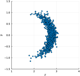
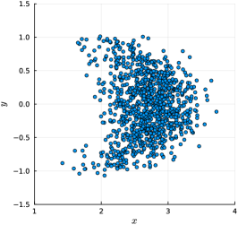
Figure 1: Visualization of the transformation of an event by a right-perturbed element of $\mathrm{SGal}(3)$, projected onto the $x$-$y$ plane. Left: perturbation to $x$ translation and $z$ rotation components only. Middle: additional (small) perturbation in time. Right: additional (large) perturbation in time. Temporal uncertainty induces a ‘spread’ in the spatial uncertainty. Each plot shows 1,000 samples drawn from a multivariate Gaussian.

9 Closing Remarks

Many problems in physics and engineering involve two (or more) inertial (or approximately inertial) reference frames that may be moving at different relative velocities and that may also be time-shifted relative to one another. The Lie group $\mathrm{SGal}(3)$ provides a natural setting for these problems and for treating the associated uncertainty; this short report provides some of the necessary mathematical machinery.

Appendix A Derivation of the Exponential Map

This appendix provides a derivation of the exponential map for $\mathrm{SGal}(3)$ in closed form. Recall that, for the square matrix $\bm{\mathbf{A}}$, the matrix exponential is defined by the power series

$$\exp\left(\bm{\mathbf{A}}\right)=\bm{\mathbf{I}}+\bm{\mathbf{A}}+\frac{1}{2!}\bm{\mathbf{A}}^{2}+\frac{1}{3!}\bm{\mathbf{A}}^{3}+\dots=\sum_{n=0}^{\infty}\frac{1}{n!}\bm{\mathbf{A}}^{n}.$$ (38)

For completeness, the matrix logarithm is defined by the power series

$$\ln\left(\bm{\mathbf{A}}\right)=\left(\bm{\mathbf{A}}-\bm{\mathbf{I}}\right)-\frac{\left(\bm{\mathbf{A}}-\bm{\mathbf{I}}\right)^{2}}{2}+\frac{\left(\bm{\mathbf{A}}-\bm{\mathbf{I}}\right)^{3}}{3}-\frac{\left(\bm{\mathbf{A}}-\bm{\mathbf{I}}\right)^{4}}{4}+\ldots=\sum_{n=1}^{\infty}(-1)^{n-1}\frac{(\bm{\mathbf{A}}-\bm{\mathbf{I}})^{n}}{n}.$$ (39)

Following 38, the exponential map from $\mathfrak{sgal}(3)$ to $\mathrm{SGal}(3)$ is

$$\exp\left(\bm{\mathbf{\xi}}^{\wedge}\right) =\sum_{n=0}^{\infty}\frac{1}{n!}\begin{bmatrix}\bm{\mathbf{\phi}}^{\wedge}&\bm{\mathbf{\nu}}&\bm{\mathbf{\rho}}\\ \bm{\mathbf{0}}&0&\iota\\ \bm{\mathbf{0}}&0&0\end{bmatrix}^{n}$$

$$=\begin{aligned} \begin{bmatrix}\,\bm{\mathbf{I}}_{3}&0&0\\ \bm{\mathbf{0}}&1&0\\ \bm{\mathbf{0}}&0&1\end{bmatrix}&+\begin{bmatrix}\bm{\mathbf{\phi}}^{\wedge}&\bm{\mathbf{\nu}}&\bm{\mathbf{\rho}}\\ \bm{\mathbf{0}}&0&\iota\\ \bm{\mathbf{0}}&0&0\end{bmatrix}\\[2.84526pt] &+\frac{1}{2!}\begin{bmatrix}\left(\bm{\mathbf{\phi}}^{\wedge}\right)^{2}\!\!&\bm{\mathbf{\phi}}^{\wedge}\!\bm{\mathbf{\nu}}\!\!&\bm{\mathbf{\phi}}^{\wedge}\!\bm{\mathbf{\rho}}+\bm{\mathbf{\nu}}\iota\\ \bm{\mathbf{0}}&0&\iota\\ \bm{\mathbf{0}}&0&0\end{bmatrix}+\frac{1}{3!}\begin{bmatrix}\left(\bm{\mathbf{\phi}}^{\wedge}\right)^{3}\!\!&\left(\bm{\mathbf{\phi}}^{\wedge}\right)^{2}\!\bm{\mathbf{\nu}}\!\!&\left(\bm{\mathbf{\phi}}^{\wedge}\right)^{2}\!\bm{\mathbf{\rho}}+\bm{\mathbf{\phi}}^{\wedge}\bm{\mathbf{\nu}}\iota\\ \bm{\mathbf{0}}&0&\iota\\ \bm{\mathbf{0}}&0&0\end{bmatrix}+\ldots\end{aligned}$$

$$=\begin{bmatrix}\bm{\mathbf{C}}&\bm{\mathbf{D}}\mspace{1.0mu}\bm{\mathbf{\nu}}&\bm{\mathbf{D}}\bm{\mathbf{\rho}}+\bm{\mathbf{E}}\mspace{1.0mu}\bm{\mathbf{\nu}}\iota\\ \bm{\mathbf{0}}&1&\iota\\ \bm{\mathbf{0}}&0&1\end{bmatrix}.$$ (40)

To determine the form of the matrices $\bm{\mathbf{C}}$, $\bm{\mathbf{D}}$, and $\bm{\mathbf{E}}$, we make use of the axis-angle rotation parameterization from Section 5 and the following identity,

$$\bm{\mathbf{u}}^{\wedge}\bm{\mathbf{u}}^{\wedge}\bm{\mathbf{u}}^{\wedge}=-\bm{\mathbf{u}}^{\wedge},$$ (41)

when $\left\|\bm{\mathbf{u}}\right\|=1$. Any power of the skew-symmetric matrix $\bm{\mathbf{u}}^{\wedge}$ greater than two can therefore be expressed in terms of $\bm{\mathbf{u}}^{\wedge}$ or $\bm{\mathbf{u}}^{\wedge}\bm{\mathbf{u}}^{\wedge}$ simply by flipping the minus sign. Returning to the problem at hand, the upper left entry in Appendix A is the exponential map from $\mathfrak{so}(3)$ to $\mathrm{SO}(3)$,

$$\bm{\mathbf{C}}=\exp\left(\bm{\mathbf{\phi}}^{\wedge}\right) =\sum_{n=0}^{\infty}\frac{1}{n!}\big{(}\phi\mspace{1.0mu}\bm{\mathbf{u}}^{\wedge}\big{)}^{n}$$

$$=\bm{\mathbf{I}}_{3}+\phi\mspace{1.0mu}\bm{\mathbf{u}}^{\wedge}+\frac{1}{2!}\phi^{2}\bm{\mathbf{u}}^{\wedge}\bm{\mathbf{u}}^{\wedge}+\frac{1}{3!}\phi^{3}\underbrace{\bm{\mathbf{u}}^{\wedge}\bm{\mathbf{u}}^{\wedge}\bm{\mathbf{u}}^{\wedge}}_{-\bm{\mathbf{u}}^{\wedge}}+\frac{1}{4!}\phi^{4}\underbrace{\bm{\mathbf{u}}^{\wedge}\bm{\mathbf{u}}^{\wedge}\bm{\mathbf{u}}^{\wedge}\bm{\mathbf{u}}^{\wedge}}_{-\bm{\mathbf{u}}^{\wedge}\bm{\mathbf{u}}^{\wedge}}+\ldots$$

$$=\bm{\mathbf{I}}_{3}+\left(\phi-\frac{1}{3!}\phi^{3}+\frac{1}{5!}\phi^{5}-\dots\right)\bm{\mathbf{u}}^{\wedge}+\left(\frac{1}{2!}\phi^{2}-\frac{1}{4!}\phi^{4}+\frac{1}{6!}\phi^{6}-\dots\right)\bm{\mathbf{u}}^{\wedge}\bm{\mathbf{u}}^{\wedge}$$

$$=\bm{\mathbf{I}}_{3}+\sin\left(\phi\right)\bm{\mathbf{u}}^{\wedge}+\big{(}1-\cos\left(\phi\right)\big{)}\bm{\mathbf{u}}^{\wedge}\bm{\mathbf{u}}^{\wedge}.$$ (42)

The remaining matrices $\bm{\mathbf{D}}$ and $\bm{\mathbf{E}}$ are

$$\bm{\mathbf{D}} =\sum_{n=0}^{\infty}\frac{1}{(n+1)!}\big{(}\phi\mspace{1.0mu}\bm{\mathbf{u}}^{\wedge}\big{)}^{n}$$

$$=\bm{\mathbf{I}}_{3}+\frac{1}{2!}\phi\mspace{1.0mu}\bm{\mathbf{u}}^{\wedge}+\frac{1}{3!}\phi^{2}\bm{\mathbf{u}}^{\wedge}\bm{\mathbf{u}}^{\wedge}+\frac{1}{4!}\phi^{3}\bm{\mathbf{u}}^{\wedge}\bm{\mathbf{u}}^{\wedge}\bm{\mathbf{u}}^{\wedge}+\frac{1}{5!}\phi^{4}\bm{\mathbf{u}}^{\wedge}\bm{\mathbf{u}}^{\wedge}\bm{\mathbf{u}}^{\wedge}\bm{\mathbf{u}}^{\wedge}+\ldots$$

$$=\bm{\mathbf{I}}_{3}+\left(\frac{1}{2!}\phi-\frac{1}{4!}\phi^{3}+\frac{1}{6!}\phi^{5}-\dots\right)\bm{\mathbf{u}}^{\wedge}+\left(\frac{1}{3!}\phi^{2}-\frac{1}{5!}\phi^{4}+\frac{1}{7!}\phi^{6}-\dots\right)\bm{\mathbf{u}}^{\wedge}\bm{\mathbf{u}}^{\wedge}$$

$$=\bm{\mathbf{I}}_{3}+\left(\frac{1-\cos\left(\phi\right)}{\phi}\right)\bm{\mathbf{u}}^{\wedge}+\left(\frac{\phi-\sin\left(\phi\right)}{\phi}\right)\bm{\mathbf{u}}^{\wedge}\bm{\mathbf{u}}^{\wedge},$$ (43)

and

$$\bm{\mathbf{E}} =\sum_{n=0}^{\infty}\frac{1}{(n+2)!}\big{(}\phi\mspace{1.0mu}\bm{\mathbf{u}}^{\wedge}\big{)}^{n}$$

$$=\frac{1}{2}\bm{\mathbf{I}}_{3}+\frac{1}{3!}\phi\mspace{1.0mu}\bm{\mathbf{u}}^{\wedge}+\frac{1}{4!}\phi^{2}\bm{\mathbf{u}}^{\wedge}\bm{\mathbf{u}}^{\wedge}+\frac{1}{5!}\phi^{3}\bm{\mathbf{u}}^{\wedge}\bm{\mathbf{u}}^{\wedge}\bm{\mathbf{u}}^{\wedge}+\frac{1}{6!}\phi^{4}\bm{\mathbf{u}}^{\wedge}\bm{\mathbf{u}}^{\wedge}\bm{\mathbf{u}}^{\wedge}\bm{\mathbf{u}}^{\wedge}+\ldots$$

$$=\frac{1}{2}\bm{\mathbf{I}}_{3}+\left(\frac{1}{3!}\phi-\frac{1}{5!}\phi^{3}+\frac{1}{7!}\phi^{5}-\dots\right)\bm{\mathbf{u}}^{\wedge}+\left(\frac{1}{4!}\phi^{2}-\frac{1}{6!}\phi^{4}+\frac{1}{8!}\phi^{6}-\dots\right)\bm{\mathbf{u}}^{\wedge}\bm{\mathbf{u}}^{\wedge}$$

$$=\frac{1}{2}\bm{\mathbf{I}}_{3}+\left(\frac{\phi-\sin\left(\phi\right)}{\phi^{2}}\right)\bm{\mathbf{u}}^{\wedge}+\left(\frac{\phi^{2}-2-2\cos\left(\phi\right)}{\phi^{2}}\right)\bm{\mathbf{u}}^{\wedge}\bm{\mathbf{u}}^{\wedge}.$$ (44)

These results are also provided (in a different format and with fewer details) in [2002_Bhand_Rigid]. Notably, by deriving the exponential map from $\mathfrak{sgal}(3)$ to $\mathrm{SGal}(3)$, we have also found closed-form solutions for the exponential map from $\mathfrak{se}(3)$ to $\mathrm{SE}(3)$ and from $\mathfrak{se_{\mathrm{2}}}(3)$ to $\mathrm{SE_{2}}(3)$ (i.e., the group of extended poses) [2022_Brossard_Associating]. We omit the details but the reader can easily check the results.

Appendix B Derivation of the Jacobian

Some additional effort is required to determine the (left) Jacobian of $\mathrm{SGal}(3)$. We derive (in closed form) several required submatrices in this appendix. The matrix $\bm{\mathbf{L}}$ is

$$\bm{\mathbf{L}} =\sum_{n=0}^{\infty}\frac{n+1}{(n+2)!}\big{(}\phi\mspace{1.0mu}\bm{\mathbf{u}}^{\wedge}\big{)}^{n}$$

$$=\frac{1}{2}\bm{\mathbf{I}}_{3}+\frac{2}{3!}\phi\mspace{1.0mu}\bm{\mathbf{u}}^{\wedge}+\frac{3}{4!}\phi^{2}\bm{\mathbf{u}}^{\wedge}\bm{\mathbf{u}}^{\wedge}+\frac{4}{5!}\phi^{3}\bm{\mathbf{u}}^{\wedge}\bm{\mathbf{u}}^{\wedge}\bm{\mathbf{u}}^{\wedge}+\frac{5}{6!}\phi^{4}\bm{\mathbf{u}}^{\wedge}\bm{\mathbf{u}}^{\wedge}\bm{\mathbf{u}}^{\wedge}\bm{\mathbf{u}}^{\wedge}+\ldots$$

$$=\frac{1}{2}\bm{\mathbf{I}}_{3}+\left(\frac{2}{3!}\phi-\frac{4}{5!}\phi^{3}+\frac{6}{7!}\phi^{5}-\dots\right)\bm{\mathbf{u}}^{\wedge}+\left(\frac{3}{4!}\phi^{2}-\frac{5}{6!}\phi^{4}+\frac{7}{8!}\phi^{6}-\dots\right)\bm{\mathbf{u}}^{\wedge}\bm{\mathbf{u}}^{\wedge}$$

$$=\frac{1}{2}\bm{\mathbf{I}}_{3}+\left(\frac{\phi\cos\left(\phi\right)-\sin\left(\phi\right)}{\phi^{2}}\right)\bm{\mathbf{u}}^{\wedge}+\left(\frac{\phi^{2}+2-2\phi\sin\left(\phi\right)-2\cos\left(\phi\right)}{2\mspace{1.0mu}\phi^{2}}\right)\bm{\mathbf{u}}^{\wedge}\bm{\mathbf{u}}^{\wedge}.\vspace*{0.25\baselineskip}$$ (45)

The matrix $\bm{\mathbf{M}}$ is more complicated. We begin by writing down the first four terms in the power series,

$$\bm{\mathbf{M}}$$