SMERF: Streamable Memory Efficient Radiance Fields
for Real-Time Large-Scene Exploration

Abstract.

Recent techniques for real-time view synthesis have rapidly advanced in fidelity and speed, and modern methods are capable of rendering near-photorealistic scenes at interactive frame rates. At the same time, a tension has arisen between explicit scene representations amenable to rasterization and neural fields built on ray marching, with state-of-the-art instances of the latter surpassing the former in quality while being prohibitively expensive for real-time applications. We introduce SMERF, a view synthesis approach that achieves state-of-the-art accuracy among real-time methods on large scenes with footprints up to 300 m² at a volumetric resolution of 3.5 mm³. Our method is built upon two primary contributions: a hierarchical model partitioning scheme, which increases model capacity while constraining compute and memory consumption, and a distillation training strategy that simultaneously yields high fidelity and internal consistency. Our method enables full six degrees of freedom navigation in a web browser and renders in real-time on commodity smartphones and laptops. Extensive experiments show that our method exceeds the state-of-the-art in real-time novel view synthesis by 0.78 dB on standard benchmarks and 1.78 dB on large scenes, renders frames three orders of magnitude faster than state-of-the-art radiance field models, and achieves real-time performance across a wide variety of commodity devices, including smartphones. We encourage readers to explore these models interactively at our project website: https://smerf-3d.github.io.

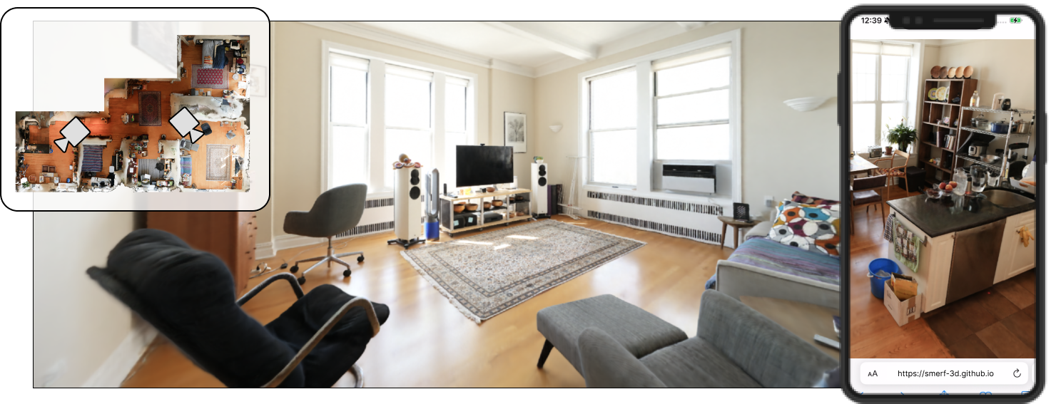
Figure 1. SMERF achieves real-time view-synthesis of large scenes on commodity devices while approaching the quality of state-of-the-art offline methods. By streaming content based on viewpoint, our method scales to hundreds of m² and runs in the browser on resource-constrained devices, including smartphones.

1. Introduction

Radiance fields have emerged as a powerful, easily-optimized representation for reconstructing and re-rendering photorealistic real-world 3D scenes. In contrast to explicit representations such as meshes and point clouds, radiance fields are often stored as neural networks and rendered using volumetric ray-marching. This is simultaneously the representation’s greatest strength and its biggest weakness: neural networks can concisely represent complex geometry and view-dependent effects given a sufficiently large computational budget. As a volumetric representation, the number of operations required to render an image scales in the number of pixels rather than the number of primitives (e.g. triangles), with the best-performing models (Barron et al., 2023) requiring tens of millions of network evaluations. As a result, real-time radiance fields make concessions in quality, speed, or representation size, and it is an open question if they can compete with alternative approaches such as Gaussian Splatting (Kerbl et al., 2023).

Our work answers this question in the affirmative. We present a scalable approach to real-time rendering of large spaces at higher fidelity than previously possible. Not only does our method approach the quality of slower, state-of-the-art models in standard benchmarks, it is the first to convincingly render unbounded, multi-room spaces in real-time on commodity hardware. Crucially, our method achieves this with a memory budget independent of scene size without compromising either image quality or rendering speed.

We use a variant of Memory-Efficient Radiance Fields (MERF) (Reiser et al., 2023), a compact representation for real-time view synthesis, as a core building block. We construct a hierarchical model architecture composed of self-contained MERF submodels, each specialized for a region of viewpoints in the scene. This greatly increases model capacity with bounded resource consumption, as only a single submodel is necessary to render any given camera. Specifically, our architecture tiles the scene with submodels to increase spatial resolution and also tiles parameters within each submodel region to more accurately model view-dependent effects. We find the increase in model capacity to be a double-edged sword, as our architecture lacks the inductive biases of state-of-the-art offline models that encourage plausible reconstructions. We therefore introduce an effective new distillation training procedure that provides abundant supervision of both color and geometry, including generalization to novel viewpoints and stable results under camera motion. These two innovations enables the real-time rendering of large scenes with similar scale and quality to existing state-of-the-art work.

Concretely, our two main contributions are:

• a tiled model architecture for real-time radiance fields capable of representing large scenes at high fidelity on hardware ranging from smartphones to desktop workstations.

• a radiance field distillation training procedure that produces highly-consistent submodels with the generalization capabilities and inductive biases of an accurate but compute-heavy teacher.

2. Related Work

Neural Radiance Fields have seen explosive progress, making a complete review challenging. Here, we only review papers directly related to our work, either as building blocks, or as sensible alternatives. Please see Tewari et al. (2022) for a comprehensive overview.

Improving NeRF’s Speed

Although NeRF produces compelling results, it is severely lacking in terms of speed: training a model takes multiple hours and rendering an image requires up to 30 seconds (Mildenhall et al., 2020). Since then, much effort has been placed on accelerating NeRF’s training and inference.

Many works achieve real-time rendering by precomputing (i.e., baking) NeRF’s view-dependent colors and opacities into sparse volumetric data structures (Hedman et al., 2021; Yu et al., 2021; Garbin et al., 2021; Yan et al., 2023). Other works show that rendering and/or training can be significantly accelerated by parameterizing a radiance field with a dense (Yu et al., 2022; Sun et al., 2022; Wu et al., 2022a), hashed (Müller et al., 2022) or low-rank voxel grid parameterization (Chan et al., 2022; Chen et al., 2022), a grid of small MLPs (Reiser et al., 2021), or a “polygon soup” of neural textures (Chen et al., 2023). Alternatively, rendering can be accelerated by reducing the sample budget while carefully allocating volumetric samples to preserve quality (Neff et al., 2021; Kurz et al., 2022; Wang et al., 2023; Gupta et al., 2023b)

In general, there is a tension between render time and memory consumption. This was explored in MERF (Reiser et al., 2023), which combines sparse and low-rank voxel grid representations to enable real-time rendering of unbounded scenes within a limited memory budget (Reiser et al., 2023). We build upon MERF and extend it to much larger environments while retaining real-time performance and adhering to the tight memory constraints of commodity devices.

Improving NeRF’s Quality

In parallel, the community has improved NeRF’s quality in a variety of ways, e.g. by eliminating aliasing (Barron et al., 2021; Hu et al., 2023), introducing efficient model architectures (Müller et al., 2022), modeling unbounded scenes (Barron et al., 2022), and eliminating floaters (Philip and Deschaintre, 2023). Other works improve robustness to other challenges, such as inaccurate camera poses (Lin et al., 2021; Song et al., 2023; Park et al., 2023), limited supervision (Niemeyer et al., 2022; Roessle et al., 2023; Wu et al., 2023a; Yang et al., 2023), or outliers including illumination changes, transient objects (Martin-Brualla et al., 2021; Rematas et al., 2022), and motion (Park et al., 2021; Jiang et al., 2023).

Most relevant for our work is Zip-NeRF (Barron et al., 2023), which uses multisampling to enable anti-aliasing for fast grid-based representations and produces accurate reconstructions of large environments while remaining tractable to train and render. Although Zip-NeRF currently achieves state-of-the-art quality on established benchmarks, a single high-resolution frame requires multiple seconds to render and the method is unsuitable for real-time rendering applications. We therefore adopt the approach of distilling a high-fidelity Zip-NeRF model into a set of MERF-based submodels, thereby achieving quality comparable to Zip-NeRF at real-time frame rates. We also incorporate several quality improvement listed above, such as latent codes for illumination variation (Martin-Brualla et al., 2021) and gradient scaling for floaters removal (Philip and Deschaintre, 2023), with no impact to rendering speed. More details can be found in App. F.

Rasterization-based View-Synthesis

While NeRF synthesises views using per-pixel ray-marching, an alternative paradigm is per-primitive rasterization leveraging specialized GPU hardware. Early such view synthesis methods approximated geometry with triangle meshes and used image blending to model view-dependent appearance (Debevec et al., 1998; Buehler et al., 2001; Davis et al., 2012). Later methods improved quality with neural appearance models (Hedman et al., 2018; Martin-Brualla et al., 2018; Liu et al., 2023) or neural mesh reconstruction (Wang et al., 2021; Yariv et al., 2023a; Rojas et al., 2023; Rakotosaona et al., 2023; Philip et al., 2021). Recent methods model detailed geometry by rasterizing overlapping meshes and either decoding (Wan et al., 2023) or compositing (Chen et al., 2023) the results. For limited viewing volumes semi-transparency can be modeled with layered representations such as multi-plane images (Penner and Zhang, 2017; Zhou et al., 2018; Flynn et al., 2019; Mildenhall et al., 2019).

GPU hardware also accelerates rendering of point-based representations. This can be leveraged to synthesize views by decoding sparse point clouds with a U-Net (Aliev et al., 2020; Wiles et al., 2020; Rückert et al., 2022). While the output views tend to be inconsistent under camera motion, this can be addressed by extending each point into a disc (Szeliski and Tonnesen, 1992; Pfister et al., 2000) equipped with a soft reconstruction kernel (Zwicker et al., 2001). Recent work showed that these soft point-based representations are amenable to gradient-based optimization and can effectively model semi-transparency as well as view-dependent appearance (Kopanas et al., 2021; Zhang et al., 2022).

Most relevant to our work is 3D Gaussian Splatting (Kerbl et al., 2023) (3DGS) which improves visual fidelity, simplifies initialization, reduces the run-time of soft point-based representations, and represents the current state-of-the-art in real-time view-synthesis. While 3DGS produces high-quality reconstructions in many scenes, optimization remains challenging, and carefully chosen heuristics are required for point allocation. This is particularly evident in large scenes, where many regions lack sufficient point density. To achieve real-time training and rendering, 3DGS further relies on platform-specific features and low-level APIs. While recent viewers display 3DGS models on commodity hardware (Kwok, 2023; Červený, 2023; Kellogg, 2024), these rely on approximations to sort order and view-dependency whose impact on quality has not yet been evaluated. Concurrent work (Fan et al., 2023; Lee et al., 2023) suffers a small reduction in visual fidelity to significantly decrease model size. In our experiments, we directly compare our cross-platform web viewer with the latest version of the official 3DGS viewer.

Large Scale NeRFs

Although NeRF models excel at reproducing objects and localized regions of a scene, they struggle to scale to larger scenes. For object-centric captures this can be ameliorated by reparameterizing the unbounded background regions of the scene to a bounded domain (Zhang et al., 2020; Barron et al., 2022). Larger, multi-room scenes can be modeled by applying anti-aliasing techniques to hash grid-backed radiance fields (Barron et al., 2023; Xu et al., 2023). Another approach is to split the scenes into multiple regions and train a separate NeRF for each region (Rebain et al., 2019; Turki et al., 2022; Wu et al., 2023b). This idea also facilitates real-time rendering of both objects (Reiser et al., 2021) and room-scale scenes (Wu et al., 2022b). Scaling to extremely large scenes such as city blocks or entire urban environments, however, requires partitioning based on camera location into redundant, overlapping scene volumes (Tancik et al., 2022; Meuleman et al., 2023). We extend the idea of camera-based partitioning to real-time view-synthesis: while existing models require expensive rendering and image blending from multiple submodels, we need only one submodel to render a given camera and leverage regularization during training to encourage mutual consistency.

Distillation and NeRF

A powerful concept in deep learning is that of distillation — training a smaller or more efficient student model to approximate the output of a more expensive or cumbersome teacher (Hinton et al., 2015; Gou et al., 2021). This idea has been successfully applied to NeRFs in a variety of contexts such as (i) distilling a large MLP into a grid of tiny MLPs (Reiser et al., 2021), (ii) distilling an expensive NeRF MLP into a small “proposal” MLP that bounds density (Barron et al., 2022), or (iii) distilling expensive secondary ray bounces into lightweight model for inverse rendering (Srinivasan et al., 2021). Distillation has also been used to obviate expensive ray marching and facilitate real-time rendering by converting an entire NeRF scene into a light field model (Wang et al., 2022; Attal et al., 2022; Cao et al., 2023; Gupta et al., 2023a) or a surface representation (Rakotosaona et al., 2023).

In this work, we distill the appearance and geometry of a large, high-quality Zip-NeRF model into a family of MERF-like submodels. Concurrently, HybridNeRF (Turki et al., 2023) also employs distillation for real-time view synthesis, albeit for a signed distance field.

3. Preliminaries

We begin with a review of MERF, which maps from 3D positions $\mathbf{x}\in\mathbb{R}^{3}$ to feature vectors $\mathbf{t}\in\mathbb{R}^{8}$. MERF parameterizes this mapping using a combination of high-resolution triplanes ($\mathbf{P}_{x}$, $\mathbf{P}_{y}$, $\mathbf{P}_{z}\in\mathbb{R}^{\mathrm{R}{\mkern 0.0mu\times\mkern 0.0mu}\mathrm{R}{\mkern 0.0mu\times\mkern 0.0mu}8}$) and a low-resolution sparse voxel grid $\mathbf{V}\in\mathbb{R}^{\mathrm{L}{\mkern 0.0mu\times\mkern 0.0mu}\mathrm{L}{\mkern 0.0mu\times\mkern 0.0mu}\mathrm{L}{\mkern 0.0mu\times\mkern 0.0mu}8}$. A query point $\mathbf{x}$ is projected on each of three axis-aligned planes and the underlying 2D grid is queried via bilinear interpolation. Additionally, a trilinear sample is taken from the sparse voxel grid. The resulting four 8-dimensional vectors are then summed:

(1) $$\mathbf{t}_{\text{MERF}}(\mathbf{x})=\mathbf{P}_{x}(\mathbf{x})+\mathbf{P}_{y}(\mathbf{x})+\mathbf{P}_{z}(\mathbf{x})+\mathbf{V}(\mathbf{x})\,.$$

This vector is then unpacked into three parts, which are independently rectified to yield a scalar density, a diffuse RGB color, and a feature vector that encodes view-dependence effects:

(2) $$\tau=\exp(\mathbf{t}_{1})\,,\quad\mathbf{c}=\operatorname{sigmoid}(\mathbf{t}_{2:4})\,,\quad\mathbf{f}=\operatorname{sigmoid}(\mathbf{t}_{5:8})\,.$$

To render a pixel, a ray is cast from that pixel’s center of projection $\mathbf{o}$ along the viewing direction $\mathbf{d}$, and sampled at a set of distances $\{t_{i}\}$ to generate a set of points along that ray $\mathbf{x}_{i}=\mathbf{o}+t_{i}\mathbf{d}$. As in NeRF (Mildenhall et al., 2020), the densities $\{\tau_{i}\}$ are converted into alpha compositing weights $\{w_{i}\}$ using the numerical quadrature approximation for volume rendering (Max, 1995):

(3) $$w_{i}=T_{i}(1-\exp(-\tau_{i}\delta_{i}))\mbox{, where }T_{i}=\exp\mathopen{}\left(-\sum\limits_{j<i}\tau_{j}\delta_{j}\mathclose{}\right)$$

where $\delta_{i}=t_{i+1}-t_{i}$ is the distance between adjacent samples. After alpha composition, the deferred shading approach of SNeRG (Hedman et al., 2021) is used to decode the blended diffuse RGB colors $\sum_{i}w_{i}\mathbf{c}_{i}$ and the blended view-dependent color features $\sum_{i}w_{i}\mathbf{f}_{i}$ into the final pixel color with the help of the small deferred rendering MLP $h(\cdot;\theta)$:

(4) $$\mathopen{}\left(\sum_{i}w_{i}\mathbf{c}_{i}\mathclose{}\right)+h\mathopen{}\left(\sum_{i}w_{i}\mathbf{c}_{i},\,\sum_{i}w_{i}\mathbf{f}_{i},\,\mathbf{d};\theta\mathclose{}\right)\,,$$

where $\theta$ are the MLP’s parameters.

In unbounded scenes, far-away content can be modelled coarsely. To achieve a resolution that drops off with the distance from the scene’s focus point, MERF applies a contraction function to each spatial position $\mathbf{x}$ before querying the feature field:

(5) $$\operatorname{contract}(\mathbf{x})_{d}=\begin{cases}x_{d}&\text{if }\|\mathbf{x}\|_{\infty}\leq 1\\ \frac{x_{d}}{\prescript{}{\phantom{d}}{\|\mathbf{x}\|_{\infty}}}&\text{if }x_{d}\neq\|\mathbf{x}\|_{\infty}>1\\ \left(2-\frac{1}{|x_{d}|}\right)\frac{x_{d}}{|x_{d}|}&\text{if }x_{d}=\|\mathbf{x}\|_{\infty}>1\end{cases}$$

4. Model

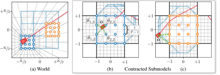
Figure 2. Coordinate systems in SMERF for a scene with $\mathrm{K}^{3}=3^{3}$ coordinate space partitions and $\mathrm{P}^{3}=4^{3}$ deferred appearance network sub-partitions. Each partition is capable of representing the entire scene while allocating the majority of its model capacity to its corresponding partition. Within each partition, we instantiate a set of spatially-anchored MLP weights $\{\theta_{i,j}\}$ parameterizing the deferred appearance model, which we trilinearly interpolate as a function of the camera origin $\mathbf{o}$ during rendering. In (a), we present the entire scene in world coordinates with the scene partition and highlight two submodels. In (b) and (c) we present the same scene from the view of two submodels in their corresponding contracted coordinate systems. (b) visualizes the rendering and parameter interpolation process when the camera origin $\mathbf{o}$ lies inside of a submodel’s partition, and (c) visualizes the same when it lies outside.

Although real-time view-synthesis methods like MERF perform well for a localized environment, they often fail to scale to large multi-room scenes. To this end, we present a hierarchical architecture: First, we partition the coordinate space of the entire scene into a series of blocks, where each block is modeled by its own MERF-like representation. Second, we introduce a grid of spatially-anchored network parameters within each block for modeling view-dependent effects. Finally, we introduce a gating mechanism for modulating high- and low-resolution contributions to a location’s feature representation. Our overall architecture can be thought of as a three-level hierarchy: based on the camera origin, (i) we select an appropriate submodel, then within a submodel (ii) we compute the parameters of a deferred appearance network via interpolation, and then within a local voxel neighborhood, (iii) we determine a location’s feature representation via feature gating.

This greatly increases the capacity of our model without diminishing rendering speed or increasing memory consumption: even as total storage requirements increase with the number of submodels, only a single submodel is needed to render a given frame. As such, when implemented on a graphics accelerator, our system maintains modest resource requirements comparable to MERF.

Coordinate Space Partitioning: While MERF offers sufficient capacity for faithfully representing medium-scale scenes, we found the use of a single set of triplanes limits its capacity and reduces image quality. In large scenes, numerous surface points project to the same 2D plane location, and the representation therefore struggles to simultaneously represent high-frequency details of multiple surfaces. Although this can be partially ameliorated by increasing the spatial resolution of the underlying representation, doing so significantly impacts memory consumption and is prohibitively expensive in practice.

We instead opt to coarsely subdivide the scene into a 3D grid based on camera origin and associate each grid cell with an independent submodel in a strategy akin to Block-NeRF (Tancik et al., 2022). Each submodel is assigned its own contraction space (Eq. 5) and is tasked with representing the region of the scene within its grid cell at high detail, while the region outside each submodel’s cell is modeled coarsely. Note that the entire scene is still represented by each submodel — the submodels differ only in terms of which portions of the scene lies inside or outside of each submodel’s contraction region. As such, rendering a camera only requires a single submodel, implying that only one submodel must be in memory at a time.

Formally, we shift and scale all training cameras to lie within a $[-\nicefrac{{\mathrm{K}}}{{2}},\nicefrac{{\mathrm{K}}}{{2}}]^{3}$ cube, and then partition this cube into $\mathrm{K}^{3}$ identical and tightly packed subvolumes of size $[-1,1]^{3}$. We assign training cameras to submodels $\{\mathcal{S}{}_{k{}}\}$ by identifying the associated subvolume $\mathbf{R}_{k{}}$ that each camera origin $\mathbf{o}$ lies within,

(6) $$s^{*}=\operatorname*{arg\,min}_{k{}\in\{1..\mathrm{K}{}^{3}\}}\mathrm{D}(\mathbf{o},k{})\mathrm{,where}\>\mathrm{D}(\mathbf{o},k{})=\min_{\mathbf{x}\in\mathbf{R}_{k{}}}||\mathbf{o}-\mathbf{x}||_{\infty}.$$

We design our camera-to-submodel assignment procedure to apply to cameras outside of the training set, ensuring its validity during test set rendering. This enables a wide range of features including ray jittering, submodel reassignment, a submodel consensus loss, arbitrary test camera placement, and ping-pong buffers as described in Sections 5 and 6.

Rather than exhaustively instantiating submodels for all $\mathrm{K}^{3}$ subvolumes, we only consider subvolumes that contain at least one training camera. As most scenes are outdoor or single-story buildings, this reduces the number of submodels from $\mathrm{K}{}^{3}$ to $O(\mathrm{K}{}^{2})$.

Deferred Appearance Network Partitioning: The second level in our partitioning hierarchy concerns the deferred rendering model. Recall that MERF employs a small multi-layer perceptron (MLP) to decode view-dependent colors from blended features as described in Eq. 4. Although the small size of this network is critical for fast inference, we observed that its capacity is insufficient to accurately reproduce complex view-dependent effects common to larger scenes. Simply increasing the size of this network is not viable as doing so would significantly reduce rendering speed.

Instead, we uniformly subdivide the domain of each submodel into a lattice with $\mathrm{P}$ vertices along each axis. We associate each cell $(u,v,w)\in\{1,..,\mathrm{P}\}^{3}$ with a separate set of network parameters $\theta_{uvw}$ and trilinearly interpolate them based on camera origin $\mathbf{o}$,

(7) $$\theta=\operatorname{Trilerp}(\mathbf{o},\{\theta_{uvw}:(u,v,w)\in\{1,..,\mathrm{P}\}^{3}\})$$

The use of trilinear interpolation, unlike the nearest-neighbor interpolation used in coordinate space partitioning, is critical in preventing aliasing of the view-dependent MLP parameters, which takes the form of conspicuous “popping” artifacts in specular highlights as the camera moves through space. We further reduce popping between submodels via regularization in Sec. 5.3. After parameter interpolation, view-dependent colors are decoded according to Eq. 4.

Since the size of the view-dependent MLP is negligible compared to total representation size, deferred network partitioning has almost no effect on memory consumption or storage impact. As a result, this technique increases model capacity almost for free. This is in contrast to coordinate space partitioning, which significantly increases storage size. We find that the union of coordinate space and deferred network partitioning is critical for effectively increasing spatial and view-dependent resolution, respectively. See Fig. 2 for an illustration of these two forms of partitioning.

Feature Gating: The final level in our hierarchy is at the level of MERF’s coarse 3D voxel grid $\mathbf{V}$ and three high-resolution planes ($\mathbf{P}_{x}$, $\mathbf{P}_{y}$, $\mathbf{P}_{z}$). In MERF, each 3D position is associated with an 8-dimensional feature vector: the sum of the contributions from these four sources (Eq. 1). Though effective, the features generated by this procedure are limited by their naive use of summation to merge high- and low-resolution information, entangling the two together.

We instead elect to use low-resolution 3D features to “gate” high-resolution features: if high-resolution features add value for a given 3D coordinate, they should be employed; otherwise, they should be ignored and the smoother, low-resolution features should be used. To this end, we modify feature aggregation as follows: instead of a naive summation, we take the last component $w(\mathbf{x})=[\mathbf{V}(\mathbf{x})]_{8}$ of the low-resolution voxel grid’s contribution and use it to scale the triplane feature contributions:

(8) $$\hat{\mathbf{t}}(\mathbf{x})=w(\mathbf{x})\cdot\left(\mathbf{P}_{x}(\mathbf{x})+\mathbf{P}_{y}(\mathbf{x})+\mathbf{P}_{z}(\mathbf{x})\right)+\mathbf{V}(\mathbf{x})\,.$$

We then build our final feature representation by concatenating the aggregated features $\hat{\mathbf{t}}(\mathbf{x})$ and the voxel grid features $\mathbf{V}(\mathbf{x})$:

(9) $$\mathbf{t}(\mathbf{x})=\hat{\mathbf{t}}(\mathbf{x})\oplus\mathbf{V}(\mathbf{x})\,.$$

Intuitively, this incentivizes the model to leverage the low-resolution voxel grid to disable the high-resolution triplanes when rendering low-frequency content such as featureless white walls, and gives the model the freedom to focus on detailed parts of the scene. This change can also be thought of as a sort of “attention”, as a multiplicative interaction is being used to determine when the model should “attend” to the triplane features (Vaswani et al., 2017). This change slightly affects the memory and speed of our model by virtue of increasing the number of rows in the first weight matrix of our MLP, but the practical impact of this is negligible.

5. Training

5.1. Radiance Field Distillation

NeRF-like models such as MERF are traditionally trained “from scratch” to minimize photometric loss on a set of posed input images. Regularization is critical when training such systems to improve generalization to novel views. One example of this is Zip-NeRF (Barron et al., 2023), which employs a family of carefully tuned losses in addition to photometric reconstruction error to achieve state-of-the-art performance on large, multi-room scenes. We instead adopt “student/teacher” distillation and train our representation to imitate an already-trained, state-of-the-art radiance field model. In particular, we use a higher-quality variant of Zip-NeRF; see App. F.

Distillation has several advantages: We inherit the helpful inductive biases of the teacher model, circumvent the need for onerous hyperparameter tuning for generalization, and enable the recovery of local representations that are also globally-consistent. We show that our approach achieves quality comparable to its Zip-NeRF teacher while being three orders of magnitude faster to render.

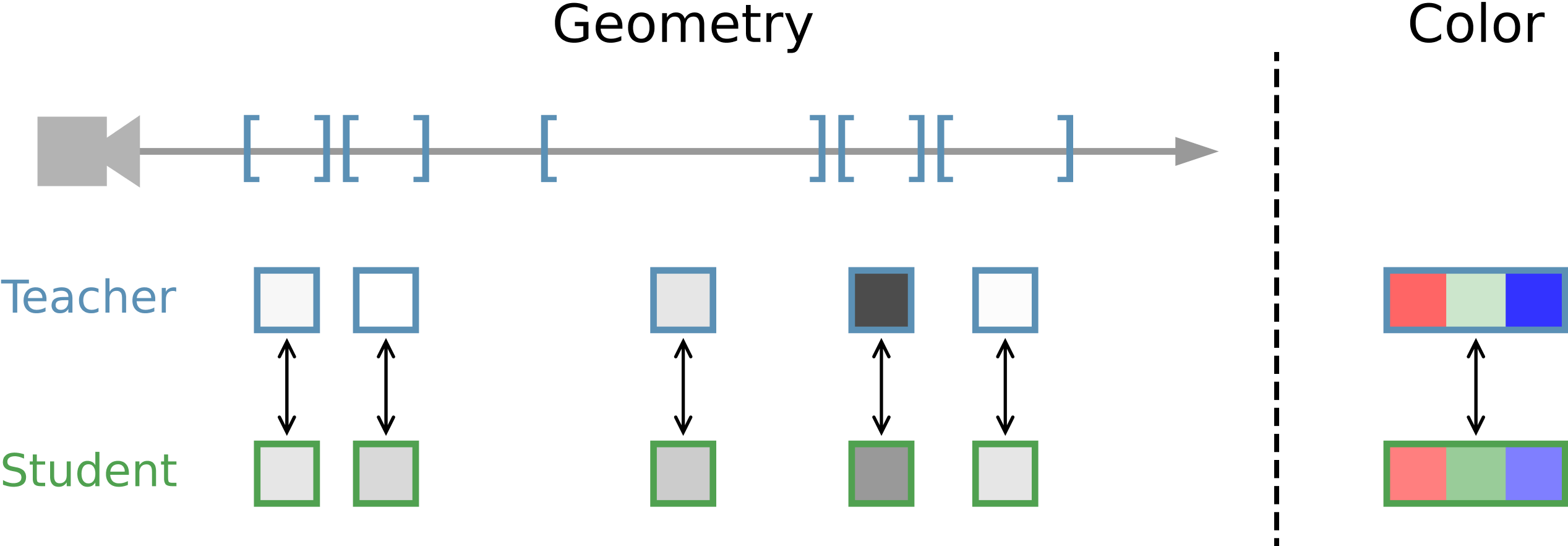
Figure 3. Teacher Supervision. The student receives photometric supervision via rendered colors and geometric supervision via the rendering weights along camera rays. Both models operate on the same set of ray intervals.

We supervise our model by distilling the appearance and geometry of a reference radiance field. Note that the teacher model is frozen during optimization. See Fig. 3 for a visualization.

Appearance: Like prior work, we supervise our model by minimizing the photometric difference between patches predicted by our model and a source of ground-truth. Instead of limiting training to a set of photos representing a small subset of a scene’s plenoptic function, our source of “ground-truth” image patches is a teacher model rendered from an arbitrary set of cameras. Specifically, we distill appearance by penalizing the discrepancy between $3{\mkern 0.0mu\times\mkern 0.0mu}3$ patches rendered from student and teacher models. We use a weighted combination of the RMSE and DSSIM (Baker et al., 2023) losses between each student patch $\mathbf{C}$ and its corresponding teacher patch $\mathbf{C}^{*}$:

(10) $$\mathcal{L}_{\mathbf{c}}=1.5\cdot\text{DSSIM}(\mathbf{C},\mathbf{C}^{*})+\sum_{\mathbf{c}\in\mathbf{C}}\left|\left|\mathbf{c}-\mathbf{\mathbf{c}}^{*}\right|\right|_{2}\,.$$

Geometry: To distill geometry, we begin by querying our teacher with a given ray origin and direction. This yields a set of weighted intervals along the camera ray $\{((t_{i},t_{i+1}),w^{T}_{i})\}$, where each $(t_{i},t_{i+1})$ are the metric distances along the ray corresponding to interval $i$, and each $w^{T}_{i}$ is the teacher’s corresponding alpha compositing weight for the same interval as per Eq. 3. The weight of each interval $i$ reflects its contribution to the final predicted radiance. It is this quantity we distill into our student. Specifically, we compute the absolute difference between the teacher and student weights:

(11) $$L_{\tau}=\sum_{i}\left|w_{i}^{T}-w_{i}^{S}\right|\,.$$

Because these volumetric rendering weights are a function of volumetric density (via Eq. 3), this loss on weights indirectly encourages the student’s and teacher’s density fields to be consistent with each other in visible regions of the scene.

5.2. Data Augmentation

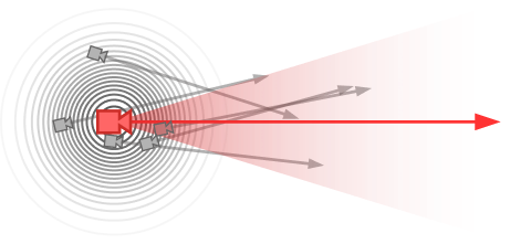
Figure 4. Ray jittering. To generate training rays for our student model (in gray) we randomly perturb the origins and directions of the camera rays used to supervise our teacher model (in red).

Because our distillation approach enables the supervision of our student model at any ray in Euclidean space, we require a procedure for selecting a useful set of rays. While sampling rays uniformly at random throughout the scene is viable, this approach leads to poor reconstruction quality as many such rays originate from inside of objects or walls or are pointed towards unimportant or under-observed parts of the scene. Using camera rays corresponding to pixels in the dataset used to train the teacher model also performs poorly, as those input images represent a tiny subset of possible views of the scene. As such, we adopt a compromise approach by using randomly-perturbed versions of the dataset’s camera rays, which yields a kind of “data augmentation” that improves generalization while focusing the student model’s attention towards the parts of the scene that the photographer deemed relevant.

To generate a training ray we first randomly select a ray from the teacher’s dataset with origin $\mathbf{o}$ and direction $\mathbf{d}$. We then jitter the origin with isotropic Gaussian noise, and draw a uniform sample from an $\epsilon$-neighborhood of the ray’s direction vector to obtain a ray $(\hat{\mathbf{o}},\hat{\mathbf{d}})$ via the E3x library (Unke and Maennel, 2024):

(12) $$\hat{\mathbf{o}} \sim\mathcal{N}(\mathbf{o},\sigma^{2}\mathbb{I}))\,,$$

(13) $$\hat{\mathbf{d}} \sim\mathcal{U}(\{\mathbf{v}\in\mathbb{R}^{3}:\left|\left|\mathbf{v}-\mathbf{d}\right|\right|_{2}<\epsilon,\left|\left|\mathbf{v}\right|\right|_{2}=1\})\,.$$

In all experiments, we set $\sigma=0.03\mathrm{K}$ and $\epsilon=0.03$. Note that $\sigma$ is defined in normalized scene coordinates, where all the input cameras are contained within the $[-\mathrm{K}/2,\mathrm{K}/2]^{3}$ cube; See Fig. 4.

5.3. Submodel Consistency

Recall that, in spite of employing a single teacher model, coordinate space partitioning means that we are effectively training multiple, independent student submodels in parallel (in practice, all submodels are trained simultaneously on a single host). This presents a challenge in terms of consistency across submodels — at test time, we seek temporal consistency under smooth camera motion, even when transitioning between submodels. This can be ameliorated by rendering multiple submodels and blending their results (Tancik et al., 2022), but doing so significantly slows rendering and requires the presence of multiple submodels at once. In contrast, we aim to render each frame while only querying a single submodel.

To encourage adjacent submodels to make similar predictions for a given camera ray, we introduce a photometric consistency loss between submodels. During training we render each camera ray in our batch twice: once using its “home” submodel $s$ (whichever submodel the ray origin lies within the interior of), and again using a randomly-chosen neighboring submodel $\hat{s}$. We then impose a straightforward loss between those two rendered colors:

(14) $$\mathcal{L}_{s} =||\mathbf{c}_{s}(\mathbf{r})-\mathbf{c}_{\hat{s}}(\mathbf{r})||_{2}\,.$$

Additionally when constructing batches of training rays, we take care to assign each ray to a submodel where it will meaningfully improve reconstruction quality. Intuitively, we expect rays to add the most value to their “home” submodel, but the rays that originate from neighboring submodels may also provide value by providing additional viewing angles of scene content within a submodel’s interior. As such, we first assign each training ray its “home” submodel, and then randomly re-assign $20\%$ of rays per batch to a randomly-selected adjacent submodel.

6. Rendering

Baking

After training we generate precomputed assets for the real-time viewer. We broadly follow the “baking” process of MERF (Reiser et al., 2023) with minor changes described in App. D. More concretely, we produce an independent set of baked assets for each submodel, where each asset collection closely mirrors that produced by MERF. Assets include three high-resolution 2D feature maps and a sparse low-resolution 3D feature grid, both represented as quantized byte arrays. Deferred network parameters, in constrast, retain their floating point representation. Unlike MERF, we store assets as gzip-compressed binary blobs, which we found slightly smaller and significantly faster to decode than PNG images.

Live Viewer

We render novel views with a custom web viewer implemented in WebGL. Particular care is taken to ensure modest compute and memory requirements, enabling real-time rendering on smartphones and other resource-constrained devices. This is primarily achieved via scene subdivision with submodels, each of which represents a localized part of the scene. In particular, a single submodel suffices to render a target camera, strongly bounding memory usage. To hide latency and ensure smooth transitions when transitioning between submodels, we employ ping-pong buffering. Further implementation details are described in App. E.

7. Experiments

We evaluate our model’s performance and quality by comparing it with two state-of-the-art methods: 3D Gaussian Splatting (Kerbl et al., 2023) and Zip-NeRF (Barron et al., 2023). Zip-NeRF produces the highest-quality reconstructions of any radiance field model but is too slow to be useful in real-time contexts, while 3DGS renders quickly but reaches a lower quality than Zip-NeRF. We show that our model, (i) is comparable to 3DGS in runtime on powerful hardware, (ii) runs in real-time on a wide range of commodity devices, and (iii) is significantly more accurate than 3DGS. We do not aim to outperform Zip-NeRF in terms of quality – it is our model’s teacher and represents an upper bound on our method’s achievable quality.

Table 1. Results on the large scenes from Zip-NeRF (Barron et al., 2023). As the spatial subdivision resolution $\mathrm{K}$ increases, our accuracy approaches that of the Zip-NeRF “teacher”.

Method	PSNR$\uparrow$	SSIM$\uparrow$	LPIPS$\downarrow$	FPS$\uparrow$	Mem (MB)$\downarrow$	Disk (MB)$\downarrow$
MERF (ours)	23.49	0.746	0.444	283	522	128
3DGS	25.50	0.810	0.369	441	227	212
Ours ($\mathrm{K}=1$)	25.44	0.777	0.412	329	505	118
Ours ($\mathrm{K}=3$)	27.09	0.823	0.350	220	1313	1628
Ours ($\mathrm{K}=5$)	27.28	0.829	0.339	204	1454	4108
Zip-NeRF	27.37	0.836	0.305	0.25∗	-

Table 2. Results on the mip-NeRF 360 dataset (Barron et al., 2022).

Method	PSNR$\uparrow$	SSIM$\uparrow$	LPIPS$\downarrow$	FPS$\uparrow$	Mem (MB)$\downarrow$	Disk (MB)$\downarrow$
BakedSDF	24.51	0.697	0.309	507	573	457
iNGP	25.68	0.706	0.302	8.61	-	104
3DGS	27.20	0.815	0.214	260	780	740
MERF (published)	25.24	0.722	0.311	162	400	162
MERF (ours)	24.95	0.728	0.302	278	504	153
Ours ($\mathrm{K}=1$)	27.98	0.818	0.212	217	466	139
Zip-NeRF	28.78	0.836	0.177	0.25∗	-

Table 3. Frame rates for different devices and resolutions, averaged across the outdoor mip-NeRF 360 scenes. Our method achieves real-time rendering rates on all platforms, including smartphones. See Table 6 for hardware specs. Not all methods are capable of running on all platforms.

	iPhone	Macbook	Desktop
Method	$380\times 640$	$1280\times 720$	$1920\times 1080$
BakedSDF	-	108	412
3DGS	-	-	176
MERF (published)	38.1	32	113
MERF (ours)	58.3	47.6	187
Ours ($\mathrm{K}=1$)	55.4	42.5

Reconstruction Quality

We first evaluate our method on four large scenes introduced by Zip-NeRF: Berlin, Alameda, London, and Nyc. Each of these scenes was captured with 1,000-2,000 photos using a $180^{\circ}$ fisheye lens. To produce an apples-to-applies comparison with 3DGS, we crop photos to a $110^{\circ}$ field-of-view and reestimate camera parameters with COLMAP (Schönberger and Frahm, 2016). Images are then downsampled to a resolution between $1392\times 793$ and $2000\times 1140$, depending on scene. Because this is a recent dataset without established benchmark results, we limit evaluations to our method, 3DGS, Zip-NeRF, and MERF. As some scenes were captured with auto-exposure enabled, we modify our algorithm and all baselines accordingly (see App. B).

The results shown in Section 7 indicate that, for modest degrees of spatial subdivision $\mathrm{K}{}$, the accuracy of our method strongly surpasses that of MERF and 3DGS. As $\mathrm{K}{}$ increases, our model’s reconstruction accuracy improves and approaches that of its Zip-NeRF teacher, with a gap of less than $0.1$ PSNR and $0.01$ SSIM at $\mathrm{K}{}=5$.

We find that these quantitative improvements understate the qualitative improvements in reconstruction accuracy, as demonstrated in Fig. 5. In large scenes, our method consistently models thin geometry, high-frequency textures, specular highlights, and far-away content where the real-time baselines fall short. At the same time, we find that increasing submodel resolution naturally increases quality, particularly with respect to high-frequency textures: see Fig. 10. In practice, we find our renders to be virtually indistinguihable from Zip-NeRF, as shown in Fig. 10.

We further evaluate our method on the mip-NeRF 360 dataset of unbounded indoor and outdoor scenes (Barron et al., 2022). These scenes are smaller in volume than those in the Zip-NeRF dataset, and as such, spatial subdivision is unnecessary to achieve high quality results. As shown in Section 7, the $\mathrm{K}{}=1$ version of our model outperforms all prior real-time models on this benchmark in terms of image quality with a rendering speed comparable to that of 3DGS. Note that we significantly improve upon the MERF baseline despite the lack of spatial subdivision, which demonstrates the value of the our deferred appearance network partitioning and feature gating contributions. Figures 6 and 10 illustrate this improvement: our method is better at representing high-frequency geometry and textures while eliminating distracting floaters and fog. Finally, in Fig. 10 you can observe how our ray jittering improves temporal stability of rendered views under camera motion.

Rendering Speed

We report frame rates at the native dataset resolution in Tables 7 and 7. We measure this by rendering each image in the test set $100\times$ on a GPU-equipped workstation and computing the arithmetic mean of frame times (i.e., the harmonic mean of FPS). See App. A for more benchmark details and results.

In Section 7, we report the performance of several recent methods as a function of image resolution and hardware platform. Our model is able to run in real-time on smartphones and laptops, albeit at reduced resolutions. MERF and BakedSDF (Yariv et al., 2023a) are also capable of running on resource-constrained platforms, but their reconstruction quality significantly lags behind ours; see Tables 7 and 7. We omit results for BakedSDF on iPhone due to memory limitations and 3DGS on iPhone and MacBook, where an official implementation for non-CUDA devices is lacking. While 3DGS modestly outperforms our cross-platform web viewer in terms of rendering speed on a desktop workstation, Tables 7 and 7 indicate that its reconstruction quality lags behind our method.

Limitations

While our method performs well in terms of quality and memory usage, it comes with a high storage cost. In the live viewer, this results in loading events and high network usage. Our method also incurs a non-trivial training cost: in addition to training the teacher, we optimize our method for 100,000-200,000 steps on 8x V100 or 16x A100 GPUs, depending on dataset. While our method achieves higher quality than 3DGS on average, it is not universally higher in detail for all parts of all scenes. We attribute this to the voxel structure imposed on the scene by our representation.

8. Conclusion

We present SMERF, a streamable, memory-efficent radiance field representation for real-time view-synthesis of large scenes. Our method renders in real-time in the web browser on everyday, resource-constrained consumer devices including smartphones and laptops. At the same time, it achieves higher quality than existing real-time methods on both medium and large scenes, exceeding the existing state-of-the-art by 0.78 and 1.78 dB PSNR, respectively.

We achieve this by distilling a high-fidelity Zip-NeRF teacher into a hierarchical student built on MERF. Our method subdivides scenes into independent submodels, each of which is further subdivided into a set of deferred rendering networks. As a consequence, only a single submodel and a local neighborhood of deferred network parameters are required to render a target view. We further improve MERF’s viewer, increasing frame rates by over 70%. As a result, memory and compute requirements remain on-par with MERF while markedly increasing quality and rendering speed. For large scenes, our quality is nearly indistinguishable from Zip-NeRF, the current state-of-the-art in offline view-synthesis. We encourage readers to explore SMERF interactively on our project webpage: https://smerf-3d.github.io.

Acknowledgements

We would like to thank Dor Verbin, Pratul Srinivasan, Ben Mildenhall, Klaus Greff, Alexey Dosovitskiy, Marcos Seefelder, and in particular Stephan Garbin for discussions and valuable feedback throughout the project. We would also like to sincerely thank Georgios Kopanas and Bernhard Kerbl for their generous help with tuning 3DGS and verifying our results. We would further like to thank Oliver Unke for his knowledge of differential geometry as applied to data augmentation and Ilies Ghanzouri for his contributions to the live renderer. Finally, we would like to thank Jane Kasdano for her valuable feedback on the design and presentation of this work.

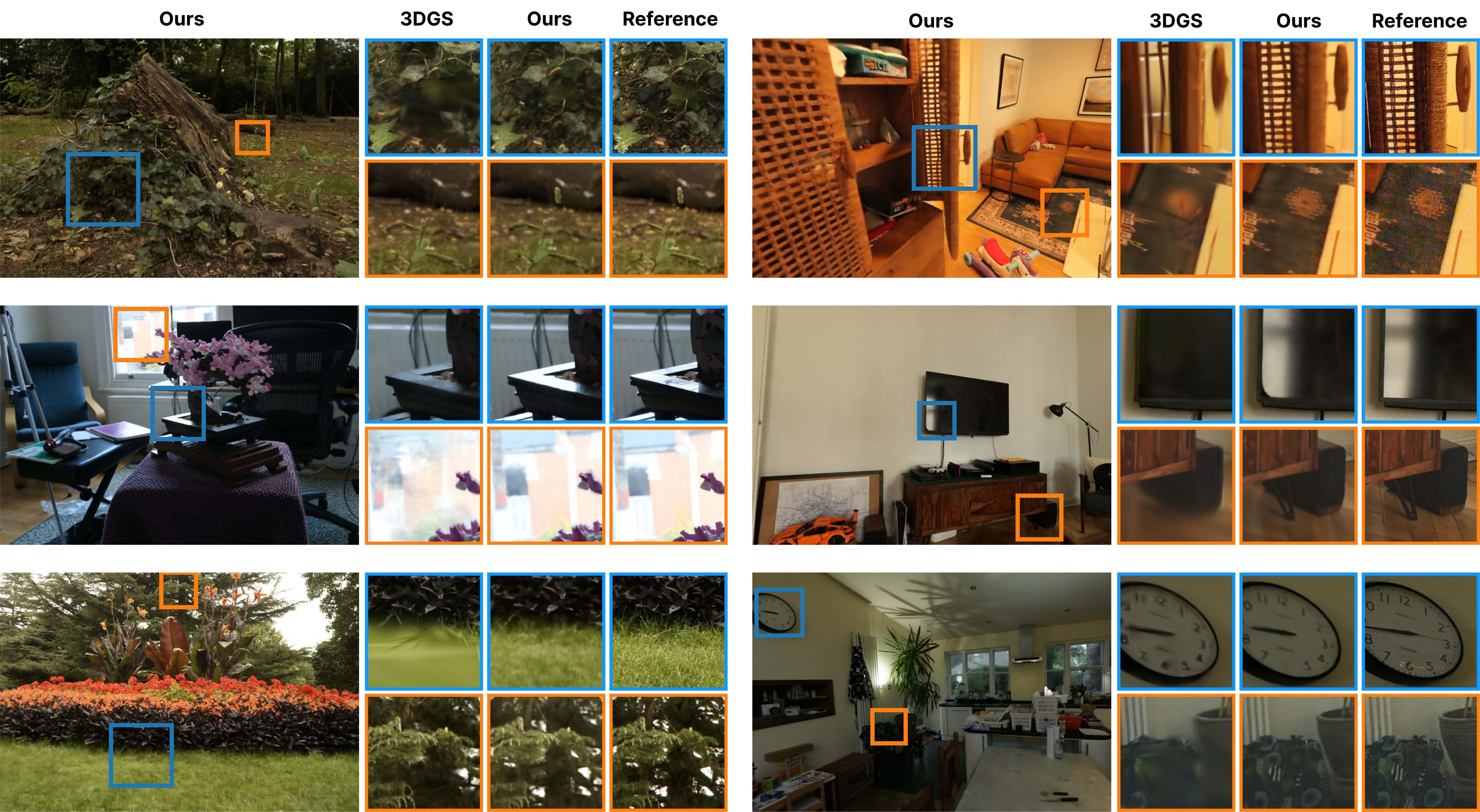
Figure 5. Qualitative comparison. We show results from our model and from 3D Gaussian Splatting (Kerbl et al., 2023) alongside ground-truth images on scenes from the mip-NeRF 360 (Barron et al., 2022) (left) and Zip-NeRF (Barron et al., 2023) (right) datasets. 3D Gaussian Splatting struggles to reproduce the thin geometry, high-frequency textures, and view-dependent effects which our model successfully recovers.

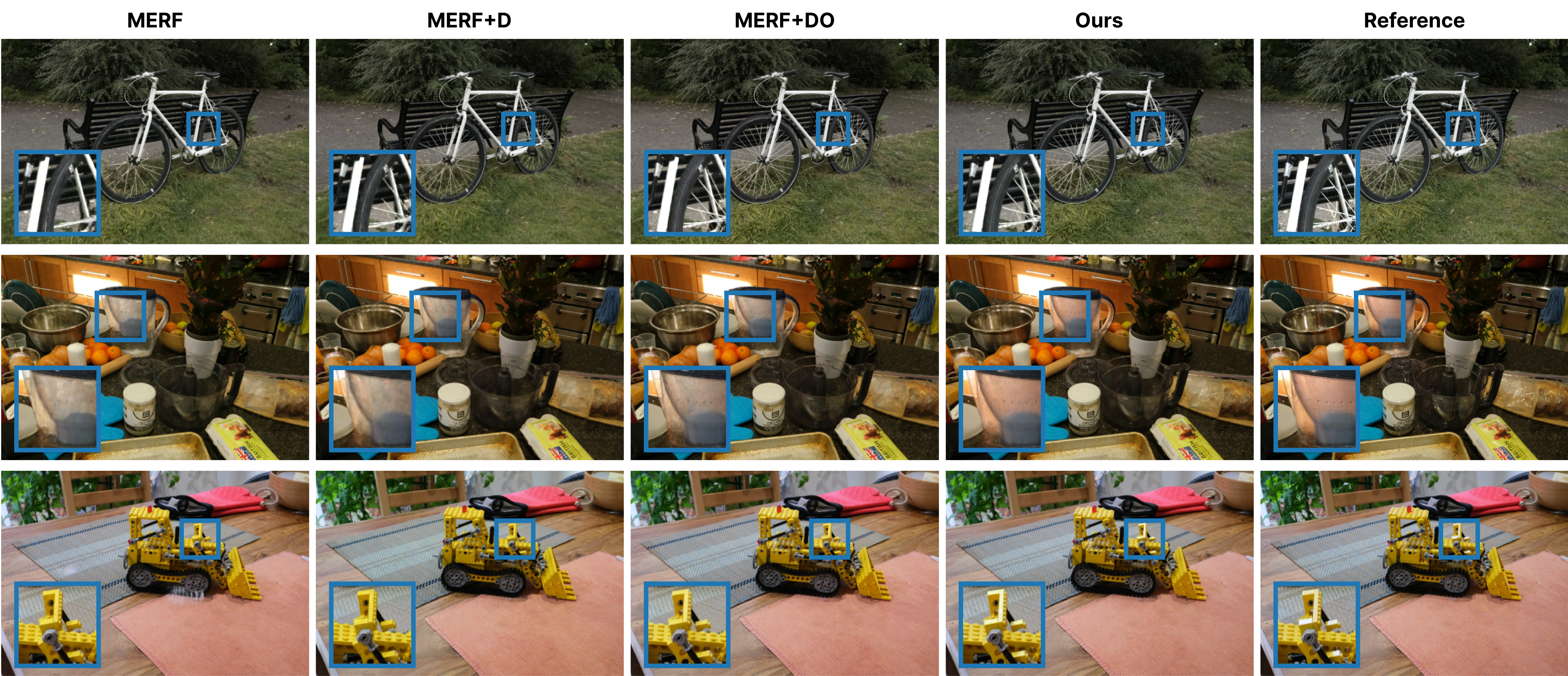
Figure 6. Feature ablations. We incrementally add distillation (MERF+D), optimization (MERF+DO), and model contributions (Ours) from Table A to MERF to reach our submodel architecture. Distillation and optimization contributions markedly increase geometric and texture detail while model contributions improve view-dependent modeling accuracy.

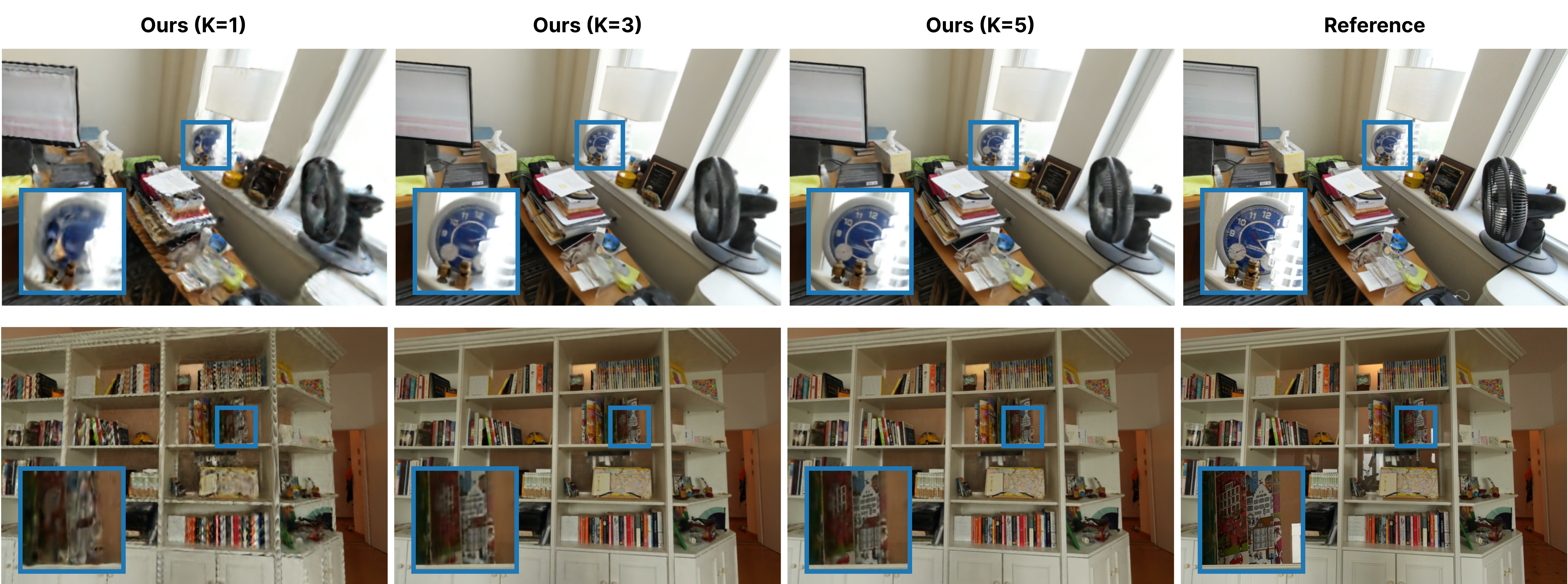
Figure 7. Submodel resolution. Increasing submodel spatial resolution leads to increased visual fidelity, particularly for high-frequency textures.

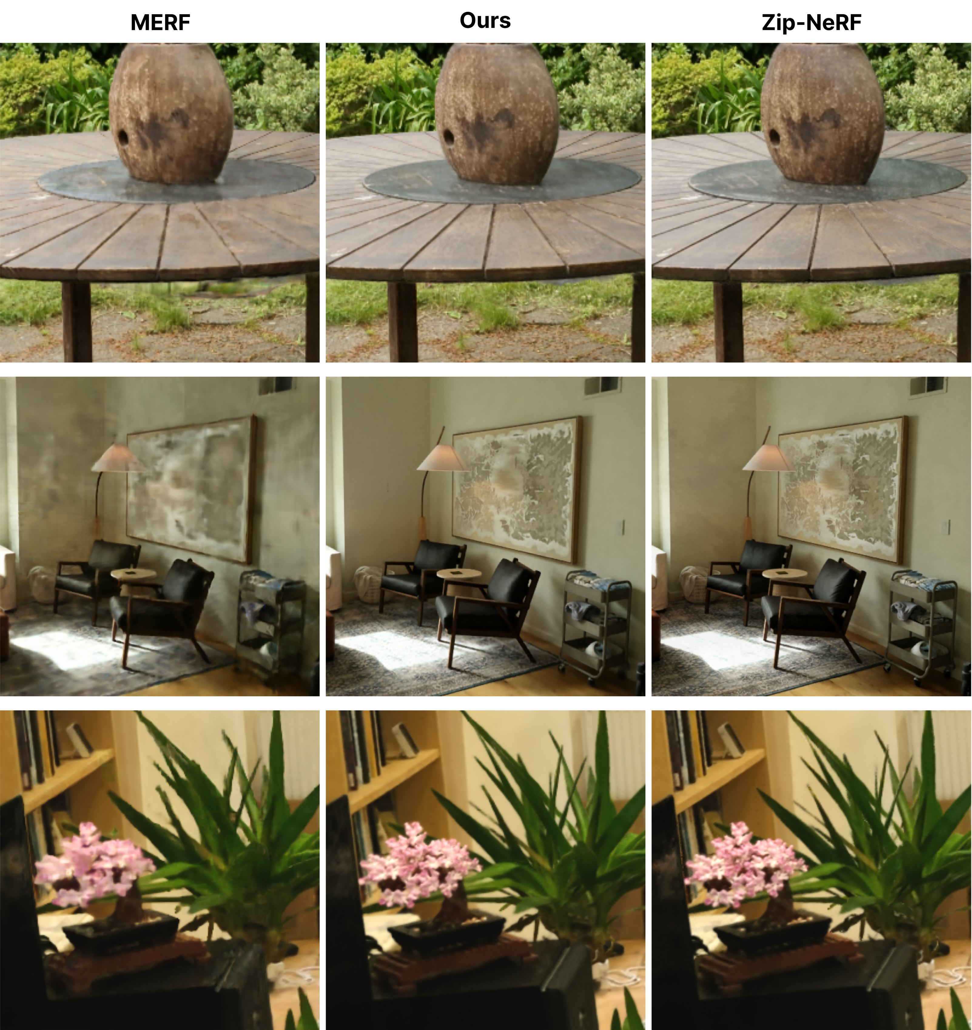
Figure 8. Comparison to Zip-NeRF. Our quality approaches that of its Zip-NeRF teacher, while MERF exhibits various artifacts (top: a “bulging” table underside, middle: “smudged” appearance, bottom: lack of geometric detail). Our method is nearly indistinguishable from Zip-NeRF.

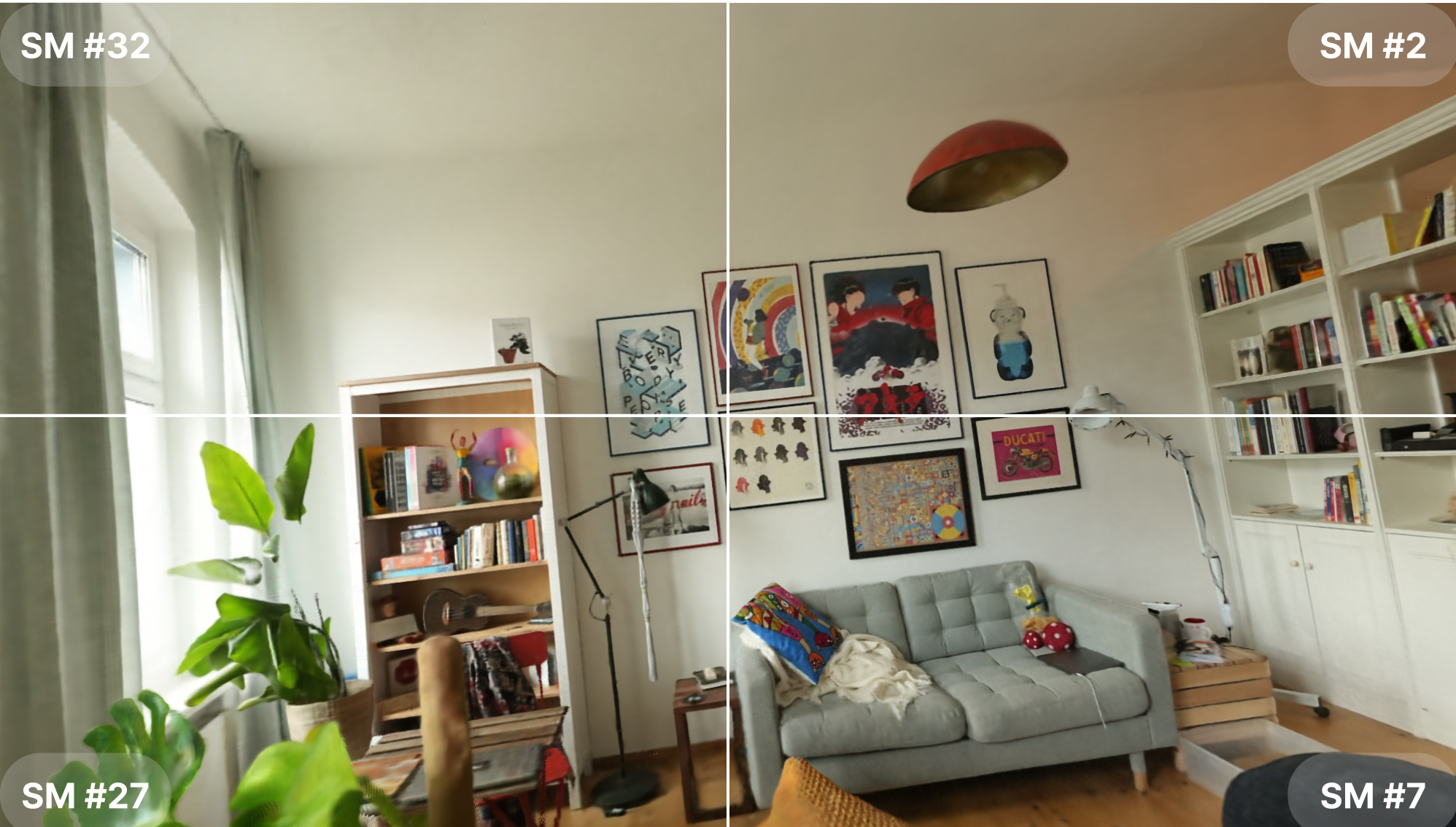
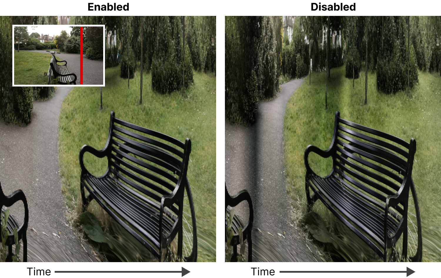
Figure 9. Submodel consistency. The same image rendered from different submodels. Despite having independent representations, our data augmentation and submodel consistency loss yield near-identical renderings.

Figure 10. Ray Jittering. Temporal consistency is demonstrated by concatenating vertical slices of a rendered video across time. Large variations in brightness correspond to flickering. We present results both with (left) and without (right) ray jittering.

Appendix A Ablations

Feature Ablations

In Appendix A, we present an ablation study demonstrating the impact of the contributions introduced in this paper. In particular, we examine the quantitative effect of independently disabling each feature on the mip-NeRF 360 dataset. We group contributions into three overarching themes: distillation training (Distill.), optimization (Optim.), and model architecture (Model). In the following, we describe each of these contributions in detail.

Distill. considers the distillation training regime described in Section 5.1. In “No Color Supervision”, we replace the teacher’s color predictions with ground truth pixels. As ground truth pixels do not support ray jittering, this feature is disabled as well. “No Geometry Supervision” replaces the teacher’s proposed ray intervals with a learned proposal network as employed in MERF. The geometry reconstruction loss of Eq. 11 is also disabled for this experiment. In “No Ray Jittering”, we disable ray jittering and restrict camera rays to those provided by the training set.

Optim. concerns changes made to the capacity and training of the core MERF architecture. In “No SSIM Loss”, we consider the effect of disabling the DSSIM loss. As patch-based inputs are no longer required, this ablation samples rays uniformly at random rather than as 3x3 patches. In “25k Train Steps”, we decrease the number of training steps from 200,000 to 25,000 to match MERF. In “No Larger Hash Grids”, we reduce the number of entries in the multi-resolution hash encoding from $N=2^{22}$ to $2^{21}$. We further decrease the depth of the MLP immediately following the hash encoding from 2 hidden layers to 1. In “No Hyperparam. Tuning”, we revert the various changes made to hyperparameters such as the hash encoding entry regularization weight, learning rate schedule, deferred network activation function, and a scaling factor applied to inputs of the contraction function (Eq. 5).

Model ablates our contributions to the model architecture. In “No MLP Grid”, we eliminate Deferred Appearance Network Partitioning as introduced in Fig. 2. In “No Total Var. Regularization”, we disable the total variation regularization term encouraging similarity between spatially-adjacent deferred network parameters. In “No Feature Gating”, we eliminate feature gating, as described in Fig. 2. In “No Median filter”, we omit the median filter applied to the high-resolution occupancy grid at baking time.

When removed one at a time, most contributions have a modest but non-negligible effect on reconstruction quality. In isolation, we find ray jittering to be the single most valuable contribution to model quality. The reason for this is apparent in Table 13: training diverges on stump when ray jittering is omitted. We attribute this to the increased capacity of our model coupled with insufficient supervision. In addition, we find hyperparameter tuning and a longer training schedule to be critical for the reconstruction of finer details, as demonstrated by a significant decrease in SSIM. The elimination of a single contribution – median filtering – has a positive impact on quality. This feature eliminates floaters and reduces baked asset size, but also introduces a slight discrepancy between the representation queried at training and rendering time.

Spatial Resolution

In Appendix A, we investigate the effects of increased spatial resolution on reconstruction quality and representation size on a variety of MERF-based baselines applied to the Zip-NeRF dataset. While SMERF’s spatial resolution may be increased by introducing additional submodels, a natural alternative is increasing the resolution of baked assets directly.

To this effect, we consider three baselines: our implementation of MERF, MERF with distillation training (MERF+D), and MERF with distillation training and model enhancements (MERF+DO). For each baseline, we increase spatial resolution by multiplying triplane and sparse feature grid resolutions by a factor of 1, 2, 3, 4, and 5 from a base resolution of $\mathrm{R}=2048$ and $\mathrm{L}=512$. We compare to SMERF, where we instead multiply submodel resolution $\mathrm{K}{}$ by the same amount, with each submodel retaining the base triplane and spares feature grid resolution. To accelerate training, we employ a reduced version of our method in this experiment: models are trained for 50,000 steps and use a multi-resolution hash grid size of $N=2^{19}$ entries per hash table.

This experiment highlights the value of model subdivision. Not only does our method consistently outperform the other model variants, memory usage of the real-time viewer grows slowly for choices of $\mathrm{K}{}>2$ and remains bounded by the size of a model’s two largest submodels (See Section 6 for details). In contrast, the memory requirements of the baselines continue to grow superlinearly with spatial resolution.

Table 4. Ablation study of our model without subdivision ($\mathrm{K}=1$) on the mip-NeRF 360 dataset (Barron et al., 2022).

		PSNR$\uparrow$	SSIM$\uparrow$	LPIPS$\downarrow$	Disk (MB)$\downarrow$
Distill.	No Color Supervision	26.45	0.775	0.259	113
	No Geometry Supervision	27.90	0.814	0.218	149
	No Ray Jittering	26.54	0.776	0.258	124
Optim.	No SSIM Loss	27.88	0.814	0.217	142
	25k Train Steps	27.56	0.803	0.231	148
	No Larger Hash Grids	27.89	0.816	0.215	145
	No Hyperparam. Tuning	27.17	0.785	0.245	148
Model	No MLP Grid	27.40	0.811	0.218	148
	No Total Var. Reg.	27.92	0.817	0.214	143
	No Feature Gating	27.63	0.809	0.221	134
	No Median filter	28.00	0.818	0.213	153
	Ours	27.98	0.818	0.212

Table 5. Spatial resolution. We compare with monolithic variants of MERF with distillation (MERF+D) and optimization (MERF+DO) contributions and varying triplane and sparse grid resolutions. Rather than directly increasing resolution, our method instead increases the submodel subdivision $\mathrm{K}{}=\{1..5\}$. Our method achieves universally higher quality and greater spatial resolution while bounding memory usage by the size of the two largest submodels. Note that this experiment uses a reduced version of our method with $2^{19}$ hash grid entries that was trained for only 50k steps.

	Spatial Res.	$2048^{3}$		$4096^{3}$		$6144^{3}$		$8192^{3}$		$10240^{3}$
	$\mathrm{K}{}$	PSNR$\uparrow$	Mem$\downarrow$	PSNR$\uparrow$	Mem$\downarrow$	PSNR$\uparrow$	Mem$\downarrow$	PSNR$\uparrow$	Mem$\downarrow$	PSNR$\uparrow$	Mem$\downarrow$
MERF (ours)	1	23.14	433	23.71	1974	23.77	5590	23.74	12119	-	-
MERF+D	1	24.14	460	24.96	2042	25.23	5745	25.28	12684	-	-
MERF+DO	1	24.43	478	25.29	2168	25.52	6061	25.59	13198	-	-
Ours	Varies	25.28	428	26.36	953	26.85	1067	26.84	1076	27.06

Appendix B Model Details

In this section, we describe the design and architecture of SMERF. We begin by describing the architecture employed in our experiments on the mip-NeRF 360 dataset. We then highlight the differences in experiments on the Zip-NeRF dataset.

mip-NeRF 360 Dataset

In this dataset, a single submodel suffices to represent an entire scene. Following MERF, our submodel consists of (i) a multi-resolution hash encoding (Müller et al., 2022) coupled with (ii) a feature-decoding MLP, followed by (iii) a deferred rendering network. For (i), we use 20 levels of hash encoding, each with $N=2^{22}$ entries and $2$ features per entry. Each level corresponds to a logarithmically-spaced resolution between $16^{3}$ and $8192^{3}$ voxels. Upon look-up and concatention, we pass these features to a feature-decoding MLP with 2 hidden layer and 64 hidden units. The MLP then produces 8 outputs corresponding to density, diffuse color, and feature preactivations. Unlike MERF, SMERF does not need to train Proposal-MLPs; instead, ray intervals are provided by the teacher.

After training, the outputs of (i) and (ii) are quantized and cached to form the triplane and sparse voxel representation used by the real-time renderer. As in MERF, we use a spatial resolution of $\mathrm{R}^{2}=2048^{2}$ for triplanes and $\mathrm{L}^{3}=512^{3}$ for sparse voxel grids (See Section 3).

Our view-dependence model follows SNeRG (Hedman et al., 2021), i.e. we predict a view-dependent residual color as a post process after volume rendering each ray. Instead of using a single view-dependence MLP, we trilinearly interpolate its parameters within a grid of $\mathrm{P}{}^{3}=5^{3}$ vertices (See Fig. 2). At each vertex, we assign parameters $\theta_{uvw}$ for an MLP with 2 hidden layers and 16 hidden units. These MLPs employ the exponential linear unit activation function (Clevert et al., 2015).

To focus our model on the center of each scene, we multiply position coordinates $\mathbf{x}$ by 2.5 before applying the contraction function in Eq. 5, i.e. $\tilde{\mathbf{x}}=2.5\,\mathbf{x}$. We find that this provides our method with significantly higher spatial fidelity in the central portion of the scene without any sharpness loss in the periphery.

Zip-NeRF Dataset

To account for the larger extent of the Zip-NeRF scenes, we fit up to $\mathrm{K}^{3}=5^{3}$ submodels per scene. As described in Fig. 2, we instantiate submodel parameters only when a training camera lies within a subvolume’s boundaries. This results in fewer than 25 instantiated submodels per scene for all of our experiments.

The architecture of each individual submodel follows the mip-NeRF 360 experiments with the following changes: First, we reduce the number of hash encoding entries per level to $N=2^{21}$ in order to reduce memory consumption during training. Second, we introduce a form of exposure conditioning inspired by Block-NeRF (Tancik et al., 2022). Specifically, we replace the rendered feature inputs to the deferred rendering network as follows,

(15) $$\hat{\mathbf{z}}(\mathbf{r}) =\operatorname{VolRend}\mathopen{}\left(\mathopen{}\left\{\sigma_{k}\mathclose{}\right\},\mathopen{}\left\{\mathbf{t}(\mathbf{x}_{k})\mathclose{}\right\}\mathclose{}\right)\,,$$

(16) $$\mathbf{z}(\mathbf{r}) =\operatorname{logit}(\hat{\mathbf{z}}(\mathbf{r}))+\log\left(\frac{\mathrm{ISO}\times\Delta t}{1000}\right)\,,$$

where $\mathrm{ISO}$ is the input image’s ISO speed rating and $\Delta t$ is the open shutter time in seconds as extracted from the training images’ metadata. In initial experiments, we fit models by instead fixing the exposure level of the teacher; however, we found visual quality lacking in scenes with large variations in illumination.

Finally, to avoid visible shearing at subvolume boundaries, we enlarge the Euclidean region of each submodel’s contracted coordinate space. Specifically, we scale the submodel position coordinates $\mathbf{x}$ by 0.8 before applying the contraction function in Eq. 5.

Appendix C Training

In this section, we describe the training of SMERF. As in App. B, we begin by describing training for mip-NeRF 360 scenes, followed by Zip-NeRF scenes.

mip-NeRF 360 Scenes

Unless otherwise stated, we optimize all models with Adam (Kingma and Ba, 2015) for 200,000 steps on 16 A100 GPUs. Our learning rate follows a cosine decay curve starting at 1e-2 and decaying to 3e-4 and our minibatches consist of 65,376 camera rays organized into 3x3 patches, where the teacher network provides 32 ray intervals per camera ray. We conserve memory by applying gradient accumulation, where each training step is accumulated over two subbatches of 32,688 camera rays.

Our models are optimized with respect to a weighted sum of the several loss functions. Photometric supervision is derived from two sources, as described in Eq. 10: (i) a per-pixel photometric RMSE loss, which encourages rendered pixels to match the teacher’s, with a weight of 1.0, and (ii) a DSSIM loss on 3x3 patches, which is added with a weight of 1.5. To adapt the DSSIM loss to smaller patch sizes, we replace the 11x11 Gaussian blur kernel with a naïve mean.

For parameter regularization, we penalize the magnitude of hash encoding entries and the variation in deferred rendering network parameters. In particular, we penalize the average squared magnitude of each hash encoding level’s parameters $\Phi_{t}\in\mathbb{R}^{N\times 2}$ using a weight of $\text{w}_{\mathrm{HG}}=0.01$, summing across different levels. Within each submodel, we further penalize the squared difference between between MLP parameters of spatially-adjacent MLPs in the deferred rendering network with a weight of $\text{w}_{\mathrm{TV}}=0.1$.

(17) $$\mathcal{L}_{\mathrm{HG}} =\text{w}_{\mathrm{HG}}\sum_{t}\frac{1}{N}\left|\left|\Phi_{t}\right|\right|_{2}^{2}$$

(18) $$\mathcal{L}_{\mathrm{TV}} =\text{w}_{\mathrm{TV}}\sum_{\Delta\in\{0,1\}^{3}}\frac{\left|\left|\theta_{uvw}-\theta_{uvw+\Delta}\right|\right|_{1}}{|\theta_{uvw}|}$$

The final loss function is thus,

(19) $$\mathcal{L} =\mathcal{L}_{\mathbf{c}}+\mathcal{L}_{\mathrm{HG}}+\mathcal{L}_{\mathrm{TV}}$$

We further regularize our models through ray jittering and random submodel reassignment. In particular, we independently perturb each camera ray by adding noise sampled from an isotropic Gaussian distribution with zero mean and $\sigma=0.03\mathrm{K}{}$. For each 3x3 patch, we further sample a random rotation matrix with $\epsilon=0.03\mathrm{K}{}$. Note that this rotation matrix is shared by all camera rays in the patch. During training, we further reassign submodels to 20% of camera rays to randomly-selected neighboring submodels (i.e. submodels whose centers are within $2$ units of the ray origin).

As in MERF, we ignore ray segments with low opacity and volumetric rendering weights. Specifically, we set the rendering weight to zero for segments whose contribution is below a threshold. We initialize this threshold to 0 between steps 0 and 80,000, and then linearly increase it from 5e-4 to 5e-3 between steps 80,000 and 160,000.

Zip-NeRF Scenes

Unlike the mip-NeRF 360 scenes, the Zip-NeRF scenes were captured with a $180^{\circ}$ field-of-view (FOV) fisheye lens. For fair comparisons with methods that do not support fisheye lenses (e.g. 3DGS), we crop these photos to a $110^{\circ}$ FOV and use COLMAP (Schönberger and Frahm, 2016) to estimate camera parameters and apply undistortion. The resulting undistorted photos have a maximum width of 4,000 pixels, which we downsample by $2\times$ for training and evaluation. This “undistorted” dataset is used for all quantitative results appearing in this work. As neither Zip-NeRF nor SMERF are limited to undistorted cameras, we employ the original fisheye dataset for our rendered videos and demos.

Training for Zip-NeRF differs from mip-NeRF 360 scenes as follows: First, we introduce a submodel consistency loss with a weight of 1.0 as described in Eq. 14, which is added to Eq. 19. Second, to reduce memory usage, we accumulate gradients over 4 batches of 16,272 rays, resulting in a total batch size of 65,088 rays. Finally, we train for 100,000 iterations, with the ray segment contribution threshold decaying between steps 40,000 and 80,000.

Appendix D Baking

mip-NeRF 360 Scenes

Our baking procedure is very similar to MERF (Reiser et al., 2023) with only minor differences. First, a 3x3x3 median filter is applied to the highest resolution occupancy grid ($\mathrm{R}^{3}=2048^{3}$) to eliminate spurious floaters. We then downsample this occupancy grid to $\mathrm{L}{}^{3}=512^{3}$ with a maximum filter and convert it to the ray marching acceleration distance grid used in App. E.

Zip-NeRF Scenes

In these scenes, we independently compute baked assets for each submodel. To accelerate baking, we only use a subset of the training cameras to construct the high-resolution occupancy grids. Recall that the world coordinate system is chosen such that cameras lie within a $[-\mathrm{K}{}/2,\mathrm{K}{}/2]^{3}$ cube. To construct a submodel’s occupancy grid, we only consider cameras whose origins lie within $1.5$ units of a submodel’s center. We further regularly subsample the camera rays by a factor of $2\times$ (i.e. every second row and column) and independently apply ray jittering to each camera ray. We find this process significantly reduces baking time with no visible impact on baked model quality.

Appendix E Real-time Rendering

Our viewer is based on the MERF volume renderer (Reiser et al., 2023), i.e. an OpenGL fragment shader that implements both ray marching and deferred rendering, using texture look-ups to retrieve feature representations and density. However, our implementation has several crucial modifications: we add support for submodels, Deferred Appearance Network interpolation, and optimized for run-time performance.

Submodels

Recall from Fig. 2 that our method only requires a single submodel to render any given viewpoint in the scene. However, to hide network latency, we “ping-pong” submodels in and out of memory as the user interactively explores the environment. When the camera moves into a new subvolume, we load the corresponding submodel into host memory, while the previous submodel, which includes an approximate representation of the geometry of this new adjacent region, continues to be used for rendering. Once the new submodel is available, we transfer it to video memory and begin using it for rendering. Peak GPU memory is thus limited to a maximum of two submodels: one actively being rendered and one being loaded into memory. We further limit host memory usage by evicting loaded submodels from memory using a least-recently-used caching scheme.

Deferred Appearance Network Interpolation

While trilinearly interpolating our deferred appearance network parameters requires additional compute, this has a negligible effect on frame render time, since it only needs to be performed only once per frame and is common to all pixels in an image. In practice, we perform this interpolation on the CPU before executing the fragment shader.

Optimizations

We introduce a variety of improvements to the MERF web viewer:

First, we compute the inputs to the Deferred Appearance MLP in a more efficient way — rather than supporting a general mapping from channel index to input feature, we instead hard code the exact input features used by our model.

Second, we define the scene parameters (e.g. grid resolutions and step sizes) as constants in the shader rather than uniform variables. This aids the shader compiler in simplifying mathematical expressions.

Finally, we use a distance grid to accelerate ray marching in free space. While MERF uses a hierarchy of binary occupancy grids to determine if a voxel is occupied or not, we use a single distance grid storing an 8-bit lower bound on the distance to the nearest occupied voxel. These distance grids thus rapidly skip large distances along each ray without resorting to expensive hierarchical ray/box intersection tests. As a result, our renderer achieves significantly higher frame rates while guaranteeing identical results.

Frame Rate Benchmarking

As the render time of most methods depend on the chosen viewpoints, we measure performance by re-rendering the test-set images in each scene. This standardizes camera parameters, pose, and resolution. For methods that rely on native low-level renderers (Müller et al., 2022; Kerbl et al., 2023), we instrument the code with GPU timers to measure the time taken to render each test-set image 100 times. We were unable to render Zip-NeRF on any of our target platforms, so we estimate frame rate based on an 8x V100 GPU configuration.

Measuring performance accurately is more challenging for the methods that use browser renderers (Yariv et al., 2023b; Reiser et al., 2023), since web browsers provide lower precision CPU-only timers, limit the maximum frame rate to the update frequency of the screen, and often round the frame time to the nearest multiple of this frequency . While disabling the frame rate limit of the browser is possible (Hedman et al., 2021), we found this to be unreliable and prone to crashes. To address this, we measure the time required to render each test set image 100 times while artificially limiting the frame rate to be lower than the update rate of the screen. We achieve this by re-rendering the output image $k$ times before scheduling it for display. Finally, to avoid reporting frame times that have been clamped to a multiple of the screen refresh rate, we measure performance with three different values for $k$ and record the smallest frame time for each test-set image.

In Section 7, we present results on three hardware platforms: iPhone, Macbook, and Desktop. The exact specifications of these platforms are presented in Table 6.

Table 6. Hardware platforms used for frame rate evaluations. Unlike other hardware platforms, iPhones use a shared CPU-GPU memory pool.

Platform	Model	RAM	GPU	VRAM
iPhone	iPhone 15 Pro (2023)	8 GB	Apple A17 Pro	-
MacBook	MacBook Pro (2019)	32 GB	AMD Radeon Pro 5500M	8 GB
Desktop	ThinkStation P620 (2021)	256 GB	NVIDIA RTX 3090	24 GB

Appendix F Zip-NeRF Teacher

To train SMERF, we employ a variation of Zip-NeRF (Barron et al., 2023) as a teacher. Unless otherwise stated, our hyperparameters match that of the original work.

mip-NeRF 360 scenes

To improve quality, we make a small number of hyperparameter changes. Our teacher models employ 10 hash grid levels with $N=2^{22}$ entries each, rather than the $2^{21}$ of the original work. We train these for twice as long (50,000 steps) with an exponentially decaying learning rate between $10^{-2}$ and $10^{-3}$. We also ramp up learning rate over 2,500, rather than 5,000, steps. Finally, to reduce floater artifacts, we incorporate Gradient Scaling (Philip and Deschaintre, 2023) with $\sigma=0.3$.

Zip-NeRF scenes

We make further adjustments to account for these larger scenes. In particular, we increase spatial resolution by adding an 11th hash grid level with a resolution of 16,384. We also train for 100,000 steps, with a final learning rate of $10^{-4}$.

One of the Zip-NeRF scenes (Alameda) was captured using varying levels of exposure. To account for this, we add Eq. 20 to the bottleneck features passed to the view-dependent MLP, as proposed in Block-NeRF (Tancik et al., 2022).

For the rendered videos and live demos, we further employ Affine Generative Latent Optimization (Barron et al., 2023), which reduces the fog and discoloration introduced by phenomena such as photographer shadows and subtle changes in weather. As the evaluation procedure for NeRF models employing GLO is still an open problem, we do not use GLO for any of the quantitative results.

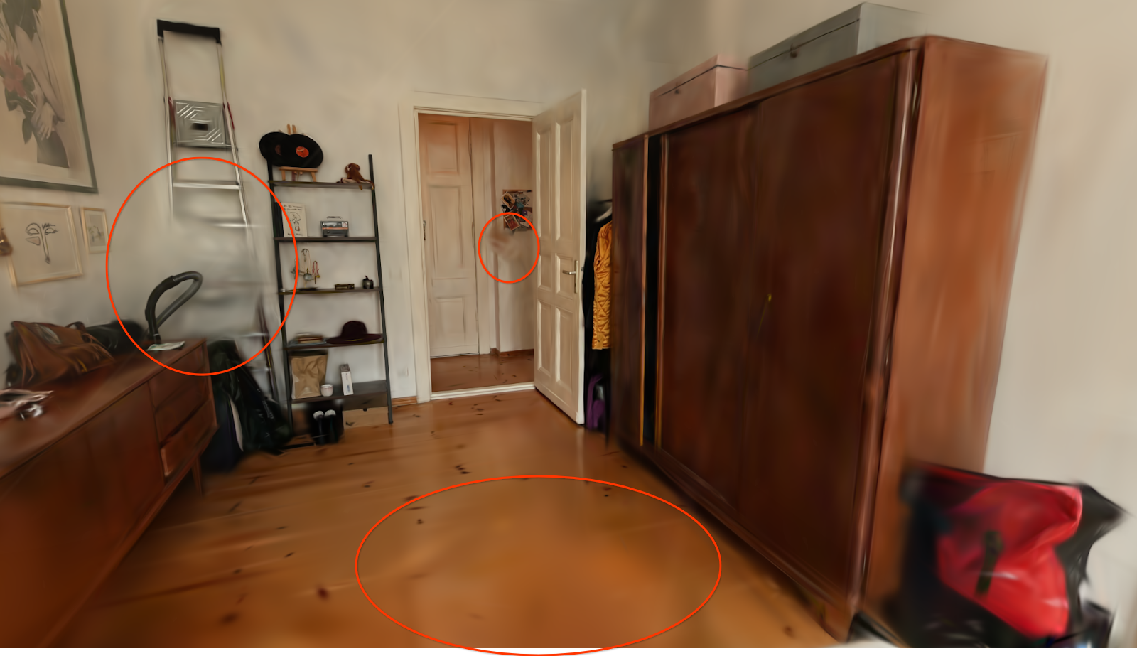
Figure 11. 3D Gaussian Splatting fails to allocate a sufficient density of Gaussian primitives in under-supervised parts of the scene.

Appendix G 3D Gaussian Splatting Experiments

In this section, we elaborate on experiments and modifications made to 3D Gaussian Splatting (3DGS) in this work.

Hyperparameter Tuning

As demonstrated in Fig. 11, 3DGS frequently struggles to allocate a sufficient density of Gaussian primitives throughout larger Zip-NeRF scenes. While we find traces of this same issue in mip-NeRF 360 scenes (See Fig. 5), the limitation become particular clear in larger captures. We believe this to be a limitation of the densification routine rather than the representation itself. Unintuitively, we find 3DGS representations for Zip-NeRF scenes to contain, on average, 3.1x fewer primitives than mip-NeRF 360 scenes, see Tables 7 and 7.

Over the course of this work, we attempted to tune a wide range of hyperparameters to fix this issue. We found that varying the number of training steps, densification steps, densification gradient thresholds, and learning rates universally reduces reconstruction quality compared to the default hyperparamters. Lowering the densification threshold increases the number of primitives as well as number of floating artifacts. In correspondences with the original authors, they affirmed that our investigations went “above and beyond what is considered best effort for comparisons.”

Exposure

To fairly compare 3DGS on the Zip-NeRF dataset, we extended the method to explicitly capture variation in camera exposure. We found that this significantly improves quality on scenes where exposure varies (Alameda). We modified 3DGS as follows:

Similarly to Eq. 16, we define exposure of image $i$ as,

(20) $$\epsilon_{i}=\log\mathopen{}\left(\frac{\mathrm{ISO}_{i}\times\Delta t_{i}}{1000}\mathclose{}\right)\,,$$

and then feed the color predicted by 3DGS and the exposure value $\epsilon_{i}$ to an MLP with 4 hidden layers and 10 units. The output of the MLP is the exposure-compensated RGB color. The MLP is optimized in the main training loop with the Adam optimizer with learning rate of $10^{-3}$.

We initialize MLP parameters via “pre-optimization”, where we bias the network towards the identity function by randomly sampling colors from the COLMAP point cloud and $\epsilon_{i}$ values from the training cameras. Given a sampled color and exposure value, the network is optimized to predict the input color. We run pre-optimization for 1,000 steps with a batch size of $2^{16}$ pixels.

For evaluation, we feed the ground-truth $\epsilon_{i}$ value to the model to obtain exposure-appropriate predictions. When rendering output videos, we use the median $\epsilon_{i}$ value across the dataset.

Appendix H Additional Results

We report PSNR, SSIM, LPIPS as well as video memory, disk usage, and frames per second for each scene in the mip-NeRF 360 and Zip-NeRF datasets. As in prior work (Barron et al., 2022; Kerbl et al., 2023), we compute LPIPS results using the implementation from Zhang et al. (2018) with the VGG back-bone and provide it with RGB pixel intensities in $[0,1]^{3}$. We benchmark frames per second results at the native test-set resolution on the “Desktop” platform descrbed in Table 6.

Table 7. PSNR on Zip-NeRF scenes.

	berlin	nyc	alameda	london
3DGS	26.60	26.41	23.52	25.45
MERF (ours)	25.27	24.82	20.34	23.53
Ours ($\mathrm{K}=1$)	26.79	25.40	23.71	25.86
Ours ($\mathrm{K}=3$)	28.41	27.88	25.17	26.90
Ours ($\mathrm{K}=5$)	28.52	28.21	25.35	27.05
Zip-NeRF	28.59	28.42	25.41	27.06

Table 8. SSIM on Zip-NeRF scenes.

	berlin	nyc	alameda	london
3DGS	0.879	0.829	0.733	0.797
MERF (ours)	0.840	0.765	0.646	0.737
Ours ($\mathrm{K}=1$)	0.852	0.771	0.701	0.789
Ours ($\mathrm{K}=3$)	0.884	0.834	0.752	0.825
Ours ($\mathrm{K}=5$)	0.887	0.844	0.758	0.829
Zip-NeRF	0.891	0.850	0.767	0.835

Table 9. LPIPS on Zip-NeRF scenes.

	berlin	nyc	alameda	london
3DGS	0.335	0.343	0.407	0.392
MERF (ours)	0.395	0.426	0.501	0.456
Ours ($\mathrm{K}=1$)	0.380	0.417	0.445	0.407
Ours ($\mathrm{K}=3$)	0.330	0.336	0.381	0.352
Ours ($\mathrm{K}=5$)	0.325	0.321	0.370	0.342
Zip-NeRF	0.297	0.281	0.338	0.304

Table 10. VRAM usage on Zip-NeRF scenes. Measured in MB.

	berlin	nyc	alameda	london
3DGS	215	270	250	168
MERF (ours)	504	466	546	571
Ours ($\mathrm{K}=1$)	472	449	511	590
Ours ($\mathrm{K}=3$)	1324	1169	1303	1456
Ours ($\mathrm{K}=5$)	1503	1400	1445	1469
Zip-NeRF	-	-	-	-

Table 11. Disk usage on Zip-NeRF scenes. Measured in MB.

	berlin	nyc	alameda	london
3DGS	202	258	239	158
MERF (ours)	105	61	160	187
Ours ($\mathrm{K}=1$)	72	47	129	226
Ours ($\mathrm{K}=3$)	1513	925	1802	2272
Ours ($\mathrm{K}=5$)	4175	3044	4675	4538
Zip-NeRF	662	662	662	662

Table 12. FPS on Zip-NeRF scenes.

	berlin	nyc	alameda	london
3DGS	339.0	416.7	467.3	625.0
MERF (ours)	184.8	469.5	269.5	348.4
Ours ($\mathrm{K}=1$)	220.3	480.8	358.4	363.6
Ours ($\mathrm{K}=3$)	140.8	314.5	236.4	273.2
Ours ($\mathrm{K}=5$)	131.4	261.8	229.9	260.4
Zip-NeRF	0.25*	0.25*	0.25*	0.25*

Table 13. PSNR on mip-NeRF 360 scenes.

	bicycle	flowers	garden	stump	treehill	room	counter	kitchen	bonsai
BakedSDF	22.04	19.53	24.94	23.59	22.25	28.68	25.69	26.72	27.17
iNGP	22.79	19.19	25.26	24.80	22.46	30.31	26.21	29.00	31.08
3DGS	25.25	21.52	27.41	26.55	22.49	30.63	28.70	30.32	31.98
MERF (published)	22.62	20.33	25.58	25.04	22.39	29.28	25.82	27.42	28.68
MERF (ours)	22.44	20.36	25.89	25.23	22.37	27.05	24.64	28.22	28.40
MERF+D	23.29	20.83	26.23	25.78	23.32	29.87	26.96	28.63	28.69
MERF+DO	25.04	21.89	26.77	26.52	23.85	30.58	27.70	30.59	30.89
Ours ($\mathrm{K}=1$)	25.58	22.24	27.66	27.19	23.93	31.38	29.02	31.68	33.19
Zip-NeRF	25.91	22.46	28.50	27.63	23.88	32.71	30.10	32.68	35.12

Table 14. SSIM on mip-NeRF 360 scenes.

	bicycle	flowers	garden	stump	treehill	room	counter	kitchen	bonsai
BakedSDF	0.570	0.452	0.751	0.595	0.559	0.870	0.808	0.817	0.851
iNGP	0.540	0.378	0.709	0.654	0.547	0.893	0.845	0.857	0.924
3DGS	0.771	0.605	0.868	0.775	0.638	0.914	0.905	0.922	0.938
MERF (published)	0.595	0.492	0.763	0.677	0.554	0.874	0.819	0.842	0.884
MERF (ours)	0.609	0.500	0.774	0.688	0.570	0.867	0.815	0.850	0.883
MERF+D	0.633	0.521	0.791	0.713	0.594	0.888	0.836	0.857	0.891
MERF+DO	0.749	0.609	0.831	0.768	0.673	0.909	0.867	0.906	0.926
Ours ($\mathrm{K}=1$)	0.760	0.626	0.844	0.784	0.682	0.918	0.892	0.916	0.941
Zip-NeRF	0.784	0.655	0.872	0.807	0.688	0.927	0.909	0.926	0.953

Table 15. LPIPS on mip-NeRF 360 scenes.

	bicycle	flowers	garden	stump	treehill	room	counter	kitchen	bonsai
BakedSDF	0.368	0.429	0.213	0.371	0.366	0.251	0.286	0.237	0.259
iNGP	0.398	0.441	0.255	0.339	0.420	0.242	0.255	0.170	0.198
3DGS	0.201	0.336	0.103	0.210	0.317	0.221	0.204	0.130	0.206
MERF (published)	0.371	0.406	0.215	0.309	0.414	0.292	0.307	0.224	0.262
MERF (ours)	0.356	0.396	0.206	0.299	0.386	0.297	0.312	0.209	0.259
MERF+D	0.334	0.388	0.191	0.284	0.361	0.264	0.286	0.204	0.250
MERF+DO	0.231	0.317	0.149	0.234	0.275	0.217	0.243	0.147	0.200
Ours ($\mathrm{K}=1$)	0.225	0.305	0.141	0.220	0.266	0.208	0.212	0.134	0.191
Zip-NeRF	0.188	0.254	0.104	0.181	0.221	0.189	0.173	0.117	0.167

Table 16. VRAM on mip-NeRF 360 scenes. Measured in MB.

	bicycle	flowers	garden	stump	treehill	room	counter	kitchen	bonsai
BakedSDF	784	879	369	681	796	287	423	475	460
iNGP	-	-	-	-	-	-	-	-	-
3DGS	1398	829	1330	1131	863	363	279	422	284
MERF (published)	291	271	198	228	1630	197	254	233	295
MERF (ours)	539	537	443	478	561	459	511	477	546
MERF+D	554	536	441	486	575	412	475	443	484
MERF+DO	508	515	435	475	546	469	485	445	448
Ours ($\mathrm{K}=1$)	502	500	431	463	530	464	467	434	439
Zip-NeRF	-	-	-	-	-	-	-	-	-

Table 17. Disk usage on mip-NeRF 360 scenes. Sizes in MB.

	bicycle	flowers	garden	stump	treehill	room	counter	kitchen	bonsai
BakedSDF	932	1039	443	808	955	296	502	568	560
iNGP	106	106	104	105	105	103	103	103	103
3DGS	1352	809	1289	1108	828	329	261	406	260
MERF (published)	207	189	114	273	188	92	136	118	167
MERF (ours)	197	197	104	144	216	99	145	120	189
MERF+D	206	188	102	153	236	57	119	96	134
MERF+DO	187	187	102	148	217	123	127	107	96
Ours ($\mathrm{K}=1$)	190	184	101	142	217	132	130	104	98
Zip-NeRF	562	562	562	562	562	562	562	562	562

Table 18. FPS on mip-NeRF 360 scenes.

	bicycle	flowers	garden	stump	treehill	room	counter	kitchen	bonsai
BakedSDF	485.4	367.6	384.6	552.5	571.4	534.8	476.2	892.9	584.8
iNGP	9.1	8.8	7.6	13.0	8.2	15.1	8.3	6.4	6.8
3DGS	177.3	342.5	288.2	218.3	401.6	168.9	321.5	311.5	303.0
MERF (published)	195.7	190.5	202.4	147.5	101.7	228.8	183.8	155.3	137.2
MERF (ours)	311.5	274.7	343.6	264.6	243.3	373.1	307.7	255.1	206.6
MERF+D	330.0	292.4	334.4	346.0	211.0	390.6	280.1	268.1	218.3
MERF+DO	253.2	224.2	223.7	258.4	243.9	336.7	244.5	186.2	148.4
Ours ($\mathrm{K}=1$)	228.3	213.2	210.1	259.1	246.9	330.0	238.1	180.8	141.0
Zip-NeRF	0.25*	0.25*	0.25*	0.25*	0.25*	0.25*	0.25*	0.25*	0.25*

References

- (1)
- Aliev et al. (2020) Kara-Ali Aliev, Artem Sevastopolsky, Maria Kolos, Dmitry Ulyanov, and Victor Lempitsky. 2020. Neural point-based graphics. Computer Vision–ECCV 2020: 16th European Conference, Glasgow, UK, August 23–28, 2020, Proceedings, Part XXII 16 (2020).
- Attal et al. (2022) Benjamin Attal, Jia-Bin Huang, Michael Zollhöfer, Johannes Kopf, and Changil Kim. 2022. Learning Neural Light Fields with Ray-Space Embedding Networks. CVPR (2022).
- Baker et al. (2023) Allison H. Baker, Alexander Pinard, and Dorit M. Hammerling. 2023. DSSIM: a structural similarity index for floating-point data. arXiv:2202.02616 [stat.CO]
- Barron et al. (2021) Jonathan T. Barron, Ben Mildenhall, Matthew Tancik, Peter Hedman, Ricardo Martin-Brualla, and Pratul P. Srinivasan. 2021. Mip-NeRF: A Multiscale Representation for Anti-Aliasing Neural Radiance Fields. ICCV (2021).
- Barron et al. (2022) Jonathan T. Barron, Ben Mildenhall, Dor Verbin, Pratul P. Srinivasan, and Peter Hedman. 2022. Mip-NeRF 360: Unbounded Anti-Aliased Neural Radiance Fields. CVPR (2022).
- Barron et al. (2023) Jonathan T. Barron, Ben Mildenhall, Dor Verbin, Pratul P. Srinivasan, and Peter Hedman. 2023. Zip-NeRF: Anti-Aliased Grid-Based Neural Radiance Fields. ICCV (2023).
- Buehler et al. (2001) Chris Buehler, Michael Bosse, Leonard McMillan, Steven Gortler, and Michael Cohen. 2001. Unstructured Lumigraph Rendering. SIGGRAPH (2001).
- Cao et al. (2023) Junli Cao, Huan Wang, Pavlo Chemerys, Vladislav Shakhrai, Ju Hu, Yun Fu, Denys Makoviichuk, Sergey Tulyakov, and Jian Ren. 2023. Real-Time Neural Light Field on Mobile Devices. CVPR (2023).
- Chan et al. (2022) Eric R. Chan, Connor Z. Lin, Matthew A. Chan, Koki Nagano, Boxiao Pan, Shalini De Mello, Orazio Gallo, Leonidas Guibas, Jonathan Tremblay, Sameh Khamis, Tero Karras, and Gordon Wetzstein. 2022. Efficient Geometry-aware 3D Generative Adversarial Networks. CVPR (2022).
- Chen et al. (2022) Anpei Chen, Zexiang Xu, Andreas Geiger, Jingyi Yu, and Hao Su. 2022. TensoRF: Tensorial Radiance Fields. ECCV (2022).
- Chen et al. (2023) Zhiqin Chen, Thomas Funkhouser, Peter Hedman, and Andrea Tagliasacchi. 2023. MobileNeRF: Exploiting the polygon rasterization pipeline for efficient neural field rendering on mobile architectures. CVPR (2023).
- Clevert et al. (2015) Djork-Arné Clevert, Thomas Unterthiner, and Sepp Hochreiter. 2015. Fast and accurate deep network learning by exponential linear units (elus). arXiv preprint arXiv:1511.07289 (2015).
- Davis et al. (2012) Abe Davis, Marc Levoy, and Fredo Durand. 2012. Unstructured Light Fields. Comput. Graph. Forum (2012).
- Debevec et al. (1998) Paul Debevec, Yizhou Yu, and George Borshukov. 1998. Efficient view-dependent image-based rendering with projective texture-mapping. EGSR (1998).
- Fan et al. (2023) Zhiwen Fan, Kevin Wang, Kairun Wen, Zehao Zhu, Dejia Xu, and Zhangyang Wang. 2023. LightGaussian: Unbounded 3D Gaussian Compression with 15x Reduction and 200+ FPS. arXiv (2023).
- Flynn et al. (2019) John Flynn, Michael Broxton, Paul Debevec, Matthew DuVall, Graham Fyffe, Ryan Overbeck, Noah Snavely, and Richard Tucker. 2019. DeepView: View synthesis with learned gradient descent. CVPR (2019).
- Garbin et al. (2021) Stephan J. Garbin, Marek Kowalski, Matthew Johnson, Jamie Shotton, and Julien Valentin. 2021. FastNeRF: High-Fidelity Neural Rendering at 200FPS. ICCV (2021).
- Gou et al. (2021) Jianping Gou, Baosheng Yu, Stephen J Maybank, and Dacheng Tao. 2021. Knowledge distillation: A survey. IJCV (2021).
- Gupta et al. (2023a) Aarush Gupta, Junli Cao, Chaoyang Wang, Ju Hu, Sergey Tulyakov, Jian Ren, and László A Jeni. 2023a. LightSpeed: Light and Fast Neural Light Fields on Mobile Devices. arXiv (2023).
- Gupta et al. (2023b) Kunal Gupta, Miloš Hašan, Zexiang Xu, Fujun Luan, Kalyan Sunkavalli, Xin Sun, Manmohan Chandraker, and Sai Bi. 2023b. MCNeRF: Monte Carlo Rendering and Denoising for Real-Time NeRFs. SIGGRAPH Asia (2023).
- Hedman et al. (2018) Peter Hedman, Julien Philip, True Price, Jan-Michael Frahm, George Drettakis, and Gabriel Brostow. 2018. Deep blending for free-viewpoint image-based rendering. SIGGRAPH Asia (2018).
- Hedman et al. (2021) Peter Hedman, Pratul P. Srinivasan, Ben Mildenhall, Jonathan T. Barron, and Paul Debevec. 2021. Baking Neural Radiance Fields for Real-Time View Synthesis. ICCV (2021).
- Hinton et al. (2015) Geoffrey Hinton, Oriol Vinyals, and Jeff Dean. 2015. Distilling the knowledge in a neural network. arXiv:1503.02531 (2015).
- Hu et al. (2023) Wenbo Hu, Yuling Wang, Lin Ma, Bangbang Yang, Lin Gao, Xiao Liu, and Yuewen Ma. 2023. Tri-miprf: Tri-mip representation for efficient anti-aliasing neural radiance fields. In Proceedings of the IEEE/CVF International Conference on Computer Vision. 19774–19783.
- Jiang et al. (2023) Yifan Jiang, Peter Hedman, Ben Mildenhall, Dejia Xu, Jonathan T Barron, Zhangyang Wang, and Tianfan Xue. 2023. AligNeRF: High-Fidelity Neural Radiance Fields via Alignment-Aware Training. In Proceedings of the IEEE/CVF Conference on Computer Vision and Pattern Recognition. 46–55.
- Kellogg (2024) Mark Kellogg. 2024. 3D Gaussian splatting for Three.js. https://github.com/mkkellogg/GaussianSplats3D.
- Kerbl et al. (2023) Bernhard Kerbl, Georgios Kopanas, Thomas Leimkühler, and George Drettakis. 2023. 3D Gaussian Splatting for Real-Time Radiance Field Rendering. SIGGRAPH (2023).
- Kingma and Ba (2015) Diederik P. Kingma and Jimmy Ba. 2015. Adam: A Method for Stochastic Optimization. ICLR (2015).
- Kopanas et al. (2021) Georgios Kopanas, Julien Philip, Thomas Leimkühler, and George Drettakis. 2021. Point-Based Neural Rendering with Per-View Optimization. Computer Graphics Forum (2021).
- Kurz et al. (2022) Andreas Kurz, Thomas Neff, Zhaoyang Lv, Michael Zollhöfer, and Markus Steinberger. 2022. AdaNeRF: Adaptive Sampling for Real-time Rendering of Neural Radiance Fields. ECCV (2022).
- Kwok (2023) Kevin Kwok. 2023. splat. https://github.com/antimatter15/splat.
- Lee et al. (2023) Joo Chan Lee, Daniel Rho, Xiangyu Sun, Jong Hwan Ko, and Eunbyung Park. 2023. Compact 3D Gaussian Representation for Radiance Field. arXiv (2023).
- Lin et al. (2021) Chen-Hsuan Lin, Wei-Chiu Ma, Antonio Torralba, and Simon Lucey. 2021. Barf: Bundle-adjusting neural radiance fields. In Proceedings of the IEEE/CVF International Conference on Computer Vision. 5741–5751.
- Liu et al. (2023) Jeffrey Yunfan Liu, Yun Chen, Ze Yang, Jingkang Wang, Sivabalan Manivasagam, and Raquel Urtasun. 2023. Real-Time Neural Rasterization for Large Scenes. CVPR (2023).
- Martin-Brualla et al. (2018) Ricardo Martin-Brualla, Rohit Pandey, Shuoran Yang, Pavel Pidlypenskyi, Jonathan Taylor, Julien Valentin, Sameh Khamis, Philip Davidson, Anastasia Tkach, Peter Lincoln, et al. 2018. Lookingood: Enhancing performance capture with real-time neural re-rendering. arXiv preprint arXiv:1811.05029 (2018).
- Martin-Brualla et al. (2021) Ricardo Martin-Brualla, Noha Radwan, Mehdi S. M. Sajjadi, Jonathan T. Barron, Alexey Dosovitskiy, and Daniel Duckworth. 2021. NeRF in the Wild: Neural Radiance Fields for Unconstrained Photo Collections. CVPR (2021).
- Max (1995) Nelson Max. 1995. Optical models for direct volume rendering. IEEE TVCG (1995).
- Meuleman et al. (2023) Andreas Meuleman, Yu-Lun Liu, Chen Gao, Jia-Bin Huang, Changil Kim, Min H. Kim, and Johannes Kopf. 2023. Progressively Optimized Local Radiance Fields for Robust View Synthesis. CVPR (2023).
- Mildenhall et al. (2019) Ben Mildenhall, Pratul P. Srinivasan, Rodrigo Ortiz-Cayon, Nima Khademi Kalantari, Ravi Ramamoorthi, Ren Ng, and Abhishek Kar. 2019. Local Light Field Fusion: Practical View Synthesis with Prescriptive Sampling Guidelines. ACM Transactions on Graphics (2019).
- Mildenhall et al. (2020) Ben Mildenhall, Pratul P. Srinivasan, Matthew Tancik, Jonathan T. Barron, Ravi Ramamoorthi, and Ren Ng. 2020. NeRF: Representing Scenes as Neural Radiance Fields for View Synthesis. ECCV (2020).
- Müller et al. (2022) Thomas Müller, Alex Evans, Christoph Schied, and Alexander Keller. 2022. Instant neural graphics primitives with a multiresolution hash encoding. SIGGRAPH (2022).
- Neff et al. (2021) Thomas Neff, Pascal Stadlbauer, Mathias Parger, Andreas Kurz, Joerg H. Mueller, Chakravarty R. Alla Chaitanya, Anton Kaplanyan, and Markus Steinberger. 2021. DONeRF: Towards Real-Time Rendering of Compact Neural Radiance Fields using Depth Oracle Networks. Computer Graphics Forum (2021).
- Niemeyer et al. (2022) Michael Niemeyer, Jonathan T. Barron, Ben Mildenhall, Mehdi S. M. Sajjadi, Andreas Geiger, and Noha Radwan. 2022. RegNeRF: Regularizing Neural Radiance Fields for View Synthesis from Sparse Inputs. CVPR (2022).
- Park et al. (2023) Keunhong Park, Philipp Henzler, Ben Mildenhall, Jonathan T. Barron, and Ricardo Martin-Brualla. 2023. CamP: Camera Preconditioning for Neural Radiance Fields. SIGGRAPH Asia (2023).
- Park et al. (2021) Keunhong Park, Utkarsh Sinha, Jonathan T. Barron, Sofien Bouaziz, Dan B Goldman, Steven M. Seitz, and Ricardo Martin-Brualla. 2021. Nerfies: Deformable Neural Radiance Fields. ICCV (2021).
- Penner and Zhang (2017) Eric Penner and Li Zhang. 2017. Soft 3D Reconstruction for View Synthesis. SIGGRAPH Asia (2017).
- Pfister et al. (2000) Hanspeter Pfister, Matthias Zwicker, Jeroen Van Baar, and Markus Gross. 2000. Surfels: Surface elements as rendering primitives. SIGGRAPH (2000).
- Philip and Deschaintre (2023) Julien Philip and Valentin Deschaintre. 2023. Floaters No More: Radiance Field Gradient Scaling for Improved Near-Camera Training. Eurographics Symposium on Rendering (2023).
- Philip et al. (2021) Julien Philip, Sébastien Morgenthaler, Michaël Gharbi, and George Drettakis. 2021. Free-viewpoint indoor neural relighting from multi-view stereo. ACM Transactions on Graphics (TOG) 40, 5 (2021), 1–18.
- Rakotosaona et al. (2023) Marie-Julie Rakotosaona, Fabian Manhardt, Diego Martin Arroyo, Michael Niemeyer, Abhijit Kundu, and Federico Tombari. 2023. NeRFMeshing: Distilling Neural Radiance Fields into Geometrically-Accurate 3D Meshes. 3DV (2023).
- Rebain et al. (2019) Daniel Rebain, Wei Jiang, Soroosh Yazdani, Ke Li, Kwang Moo Yi, and Andrea Tagliasacchi. 2019. DeRF: Decomposed Radiance Fields. CVPR (2019).
- Reiser et al. (2021) Christian Reiser, Songyou Peng, Yiyi Liao, and Andreas Geiger. 2021. KiloNeRF: Speeding up neural radiance fields with thousands of tiny MLPs. ICCV (2021).
- Reiser et al. (2023) Christian Reiser, Richard Szeliski, Dor Verbin, Pratul P. Srinivasan, Ben Mildenhall, Andreas Geiger, Jonathan T. Barron, and Peter Hedman. 2023. MERF: Memory-Efficient Radiance Fields for Real-time View Synthesis in Unbounded Scenes. SIGGRAPH (2023).
- Rematas et al. (2022) Konstantinos Rematas, Andrew Liu, Pratul P Srinivasan, Jonathan T Barron, Andrea Tagliasacchi, Thomas Funkhouser, and Vittorio Ferrari. 2022. Urban radiance fields. In Proceedings of the IEEE/CVF Conference on Computer Vision and Pattern Recognition. 12932–12942.
- Roessle et al. (2023) Barbara Roessle, Norman Müller, Lorenzo Porzi, Samuel Rota Bulò, Peter Kontschieder, and Matthias Nießner. 2023. GANeRF: Leveraging Discriminators to Optimize Neural Radiance Fields. SIGGRAPH Asia (2023).
- Rojas et al. (2023) Sara Rojas, Jesus Zarzar, Juan C Pérez, Artsiom Sanakoyeu, Ali Thabet, Albert Pumarola, and Bernard Ghanem. 2023. Re-ReND: Real-time rendering of NeRFs across devices. CVPR (2023).
- Rückert et al. (2022) Darius Rückert, Linus Franke, and Marc Stamminger. 2022. ADOP: Approximate differentiable one-pixel point rendering. SIGGRAPH (2022).
- Schönberger and Frahm (2016) Johannes Lutz Schönberger and Jan-Michael Frahm. 2016. Structure-from-Motion Revisited. CVPR (2016).
- Song et al. (2023) Liang Song, Guangming Wang, Jiuming Liu, Zhenyang Fu, Yanzi Miao, et al. 2023. SC-NeRF: Self-Correcting Neural Radiance Field with Sparse Views. arXiv preprint arXiv:2309.05028 (2023).
- Srinivasan et al. (2021) Pratul P. Srinivasan, Boyang Deng, Xiuming Zhang, Matthew Tancik, Ben Mildenhall, and Jonathan T. Barron. 2021. NeRV: Neural Reflectance and Visibility Fields for Relighting and View Synthesis. CVPR (2021).
- Sun et al. (2022) Cheng Sun, Min Sun, and Hwann-Tzong Chen. 2022. Direct voxel grid optimization: Super-fast convergence for radiance fields reconstruction. CVPR (2022).
- Szeliski and Tonnesen (1992) Richard Szeliski and David Tonnesen. 1992. Surface modeling with oriented particle systems. SIGGRAPH (1992).
- Tancik et al. (2022) Matthew Tancik, Vincent Casser, Xinchen Yan, Sabeek Pradhan, Ben Mildenhall, Pratul Srinivasan, Jonathan T. Barron, and Henrik Kretzschmar. 2022. Block-NeRF: Scalable Large Scene Neural View Synthesis. CVPR (2022).
- Tewari et al. (2022) Ayush Tewari, Justus Thies, Ben Mildenhall, Pratul Srinivasan, Edgar Tretschk, W Yifan, Christoph Lassner, Vincent Sitzmann, Ricardo Martin-Brualla, Stephen Lombardi, et al. 2022. Advances in neural rendering. Computer Graphics Forum (2022).
- Turki et al. (2023) Haithem Turki, Vasu Agrawal, Samuel Rota Bulò, Lorenzo Porzi, Peter Kontschieder, Deva Ramanan, Michael Zollhöfer, and Christian Richardt. 2023. HybridNeRF: Efficient Neural Rendering via Adaptive Volumetric Surfaces. arXiv (2023).
- Turki et al. (2022) Haithem Turki, Deva Ramanan, and Mahadev Satyanarayanan. 2022. Mega-NERF: Scalable Construction of Large-Scale NeRFs for Virtual Fly-Throughs. CVPR (2022).
- Unke and Maennel (2024) Oliver T. Unke and Hartmut Maennel. 2024. E3x: -Equivariant Deep Learning Made Easy. arXiv preprint arXiv:2401.07595 (2024).
- Vaswani et al. (2017) Ashish Vaswani, Noam Shazeer, Niki Parmar, Jakob Uszkoreit, Llion Jones, Aidan N Gomez, Łukasz Kaiser, and Illia Polosukhin. 2017. Attention is all you need. NeurIPS (2017).
- Wan et al. (2023) Ziyu Wan, Christian Richardt, Aljaž Božič, Chao Li, Vijay Rengarajan, Seonghyeon Nam, Xiaoyu Xiang, Tuotuo Li, Bo Zhu, Rakesh Ranjan, and Jing Liao. 2023. Learning Neural Duplex Radiance Fields for Real-Time View Synthesis. CVPR (2023).
- Wang et al. (2022) Huan Wang, Jian Ren, Zeng Huang, Kyle Olszewski, Menglei Chai, Yun Fu, and Sergey Tulyakov. 2022. R2L: Distilling Neural Radiance Field to Neural Light Field for Efficient Novel View Synthesis. ECCV (2022).
- Wang et al. (2021) Peng Wang, Lingjie Liu, Yuan Liu, Christian Theobalt, Taku Komura, and Wenping Wang. 2021. NeuS: Learning Neural Implicit Surfaces by Volume Rendering for Multi-view Reconstruction. NeurIPS (2021).
- Wang et al. (2023) Zian Wang, Tianchang Shen, Merlin Nimier-David, Nicholas Sharp, Jun Gao, Alexander Keller, Sanja Fidler, Thomas Müller, and Zan Gojcic. 2023. Adaptive Shells for Efficient Neural Radiance Field Rendering. SIGGRAPH Asia (2023).
- Wiles et al. (2020) Olivia Wiles, Georgia Gkioxari, Richard Szeliski, and Justin Johnson. 2020. SynSin: End-to-End View Synthesis From a Single Image. CVPR (2020).
- Wu et al. (2022a) Liwen Wu, Jae Yong Lee, Anand Bhattad, Yuxiong Wang, and David Forsyth. 2022a. DIVeR: Real-time and Accurate Neural Radiance Fields with Deterministic Integration for Volume Rendering. CVPR (2022).
- Wu et al. (2023a) Rundi Wu, Ben Mildenhall, Philipp Henzler, Keunhong Park, Ruiqi Gao, Daniel Watson, Pratul P. Srinivasan, Dor Verbin, Jonathan T. Barron, Ben Poole, and Aleksander Holynski. 2023a. ReconFusion: 3D Reconstruction with Diffusion Priors. arXiv (2023).
- Wu et al. (2023b) Xiuchao Wu, Jiamin Xu, Xin Zhang, Hujun Bao, Qixing Huang, Yujun Shen, James Tompkin, and Weiwei Xu. 2023b. ScaNeRF: Scalable Bundle-Adjusting Neural Radiance Fields for Large-Scale Scene Rendering. ACM Transactions on Graphics (TOG) (2023).
- Wu et al. (2022b) Xiuchao Wu, Jiamin Xu, Zihan Zhu, Hujun Bao, Qixing Huang, James Tompkin, and Weiwei Xu. 2022b. Scalable Neural Indoor Scene Rendering. ACM TOG (2022).
- Xu et al. (2023) Linning Xu, Vasu Agrawal, William Laney, Tony Garcia, Aayush Bansal, Changil Kim, Samuel Rota Bulò, Lorenzo Porzi, Peter Kontschieder, Aljaž Božič, Dahua Lin, Michael Zollhöfer, and Christian Richardt. 2023. VR-NeRF: High-Fidelity Virtualized Walkable Spaces. SIGGRAPH Asia (2023).
- Yan et al. (2023) Han Yan, Celong Liu, Chao Ma, and Xing Mei. 2023. PlenVDB: Memory Efficient VDB-Based Radiance Fields for Fast Training and Rendering. In CVPR.
- Yang et al. (2023) Jiawei Yang, Marco Pavone, and Yue Wang. 2023. FreeNeRF: Improving Few-shot Neural Rendering with Free Frequency Regularization. In Proceedings of the IEEE/CVF Conference on Computer Vision and Pattern Recognition. 8254–8263.
- Yariv et al. (2023a) Lior Yariv, Peter Hedman, Christian Reiser, Dor Verbin, Pratul P. Srinivasan, Richard Szeliski, Jonathan T. Barron, and Ben Mildenhall. 2023a. BakedSDF: Meshing Neural SDFs for Real-Time View Synthesis. SIGGRAPH (2023).
- Yariv et al. (2023b) Lior Yariv, Peter Hedman, Christian Reiser, Dor Verbin, Pratul P. Srinivasan, Richard Szeliski, Jonathan T. Barron, and Ben Mildenhall. 2023b. BakedSDF: Meshing Neural SDFs for Real-Time View Synthesis. SIGGRAPH (2023).
- Yu et al. (2022) Alex Yu, Sara Fridovich-Keil, Matthew Tancik, Qinhong Chen, Benjamin Recht, and Angjoo Kanazawa. 2022. Plenoxels: Radiance fields without neural networks. CVPR (2022).
- Yu et al. (2021) Alex Yu, Ruilong Li, Matthew Tancik, Hao Li, Ren Ng, and Angjoo Kanazawa. 2021. PlenOctrees for real-time rendering of neural radiance fields. ICCV (2021).
- Zhang et al. (2020) Kai Zhang, Gernot Riegler, Noah Snavely, and Vladlen Koltun. 2020. NeRF++: Analyzing and Improving Neural Radiance Fields. arXiv:2010.07492 (2020).
- Zhang et al. (2022) Qiang Zhang, Seung-Hwan Baek, Szymon Rusinkiewicz, and Felix Heide. 2022. Differentiable Point-Based Radiance Fields for Efficient View Synthesis. SIGGRAPH Asia (2022).
- Zhang et al. (2018) Richard Zhang, Phillip Isola, Alexei A Efros, Eli Shechtman, and Oliver Wang. 2018. The Unreasonable Effectiveness of Deep Features as a Perceptual Metric. In CVPR.
- Zhou et al. (2018) Tinghui Zhou, Richard Tucker, John Flynn, Graham Fyffe, and Noah Snavely. 2018. Stereo Magnification: Learning View Synthesis using Multiplane Images. SIGGRAPH (2018).
- Zwicker et al. (2001) Matthias Zwicker, Hanspeter Pfister, Jeroen Van Baar, and Markus Gross. 2001. Surface splatting. SIGGRAPH (2001).
- Červený (2023) Jakub Červený. 2023. gsplat — 3D Gaussian Splatting WebGL viewer. https://gsplat.tech/.