Improved Frequency Estimation Algorithms with and without Predictions

Abstract

Estimating frequencies of elements appearing in a data stream is a key task in large-scale data analysis. Popular sketching approaches to this problem (e.g., CountMin and CountSketch) come with worst-case guarantees that probabilistically bound the error of the estimated frequencies for any possible input. The work of Hsu et al. (2019) introduced the idea of using machine learning to tailor sketching algorithms to the specific data distribution they are being run on. In particular, their learning-augmented frequency estimation algorithm uses a learned heavy-hitter oracle which predicts which elements will appear many times in the stream. We give a novel algorithm, which in some parameter regimes, already theoretically outperforms the learning based algorithm of Hsu et al. without the use of any predictions. Augmenting our algorithm with heavy-hitter predictions further reduces the error and improves upon the state of the art. Empirically, our algorithms achieve superior performance in all experiments compared to prior approaches.

1 Introduction

In frequency estimation, we stream a sequence of elements from $[n]:=\{1,\ldots,n\}$, and the goal is to estimate $f_{i}$, the frequency of the $i$th element, at the end of the stream using low-space. Frequency estimation is one of the central problems in data streaming with a wide range of applications from networking (gathering important monitoring statistics [31, 62, 46]) to machine learning (NLP [33], feature selection [3], semi supervised learning [58]). CountMin (CM) [20] and CountSketch (CS) [14] are arguably the most popular and versatile of the algorithms for frequency estimation, and are implemented in many popular packages such as Spark [63], Twitter Algebird [10], and Redis.

Standard approaches to frequency estimation are designed to perform well in the worst-case due to the multitudinous benefits of worst-case guarantees. However, algorithms designed to handle any possible input do not exploit special structure of the particular distribution of inputs they are used for. In practice, these patterns can be described by domain experts or learned from historical data. Following the burgeoning trend of combining machine learning and classical algorithm design, [36] initiated the study of learning-augmented frequency estimation by extending the classical CM and CS algorithms in a simple but effective manner via a heavy-hitters oracle. During a training phase, they construct a classifier (e.g. a neural network) to detect whether an element $i$ is “heavy” (e.g., whether $f_{i}$ is among the most frequent items). After such a classifier is trained, they scan the input stream, and apply the classifier to each element $i$. If the element is predicted to be heavy, it is allocated a unique bucket, so that an exact value of $f_{i}$ is computed. Otherwise, the stream element is inputted into the standard sketching algorithms.

The advantage of their algorithm was analyzed under the assumption that the true frequencies follow a heavy-tailed Zipfian distribution. This is a common and natural reoccurring pattern in real world data where there are a few very frequent elements and many infrequent elements. Experimentally, [36] showed several real datasets where the Zipfian assumption (approximately) held and useful heavy-hitter oracles could be trained in practice. Our paper is motivated by the following natural questions and goals in light of prior works:

Can we design better frequency estimation algorithms (with and without predictions) for heavy-tailed distributions?

In particular, we consider the setting of [36] where the underlying data follow a heavy-tailed distribution and investigate whether sketching algorithms can be further tailored for such distributions. Before tackling this question, we must tightly characterize the benefits–and limitations–of these existing methods, which is another goal of our paper:

Give tight error guarantees for CountMin and CountSketch, as well as their learning-augmented variants, on Zipfian data.

Lastly, any algorithms we design must possess worst case bounds in the case that either the data does not match our Zipfian (or more generally, heavy-tailed) assumption or the learned predictions have high error, leading to the following ‘best of both worlds’ goal:

Design algorithms which exploit heavy tailed distributions and ML predictions but also maintain worst-case guarantees.

We addresses these challenges and goals and our contributions can be summarized as follows:

• We give tight upper and lower bounds for CM and CS, with and without predictions, for heavy tailed distributions. A surprising conclusion from our analysis is that (for a natural error metric) a constant number of rows is optimal for both CM and CS. In addition, our theoretical analysis shows that CS outperforms CM, both with and without predictions, validating the experimental results of [36].

• We go beyond CM and CS based algorithms to give a better frequency estimation algorithm for heavy tailed distributions, with and without the use of predictions. We show that our algorithms can deliver up to a logarithmic factor improvement in the error bound over CS and its learned variant. In addition, our algorithm has worst case guarantees.

• Prior learned approaches require querying an oracle for every element in the stream. In contrast, we obtain a parsimonious version of our algorithm which only requires a limited number of queries to the oracle. The number of queries we use is approximately equal to the given space budget.

• Lastly, we evaluate our algorithms on two real-world datasets with and without ML based predictions and show superior empirical performance compared to prior work in all cases.

1.1 Preliminaries

Notation and Estimation Error

The stream updates an $n$ dimensional frequency vector and every stream element is of the form $(i,\Delta)$ where $i\in[n]$ and $\Delta\in\mathbb{R}$ denotes the update on the coordinate. The final frequency vector is denoted as $f\in\mathbb{R}^{n}$. Let $N=\sum_{i\in[n]}f_{i}$ denote the sum of all frequencies. To simplify notation, we assume that $f_{1}\geq f_{2}\geq\ldots\geq f_{n}$. $\tilde{f}_{i}$ denotes the estimate of the frequency $f_{i}$. Given estimates $\{\tilde{f}_{i}\}_{i\in[n]}$, the error of a particular frequency is $|\tilde{f}_{i}-f_{i}|$. We also consider the following notion of overall weighted error as done in [36]:

$$\text{Weighted Error:}=\frac{1}{N}\sum_{i\in[n]}f_{i}\cdot|\tilde{f}_{i}-f_{i}|.$$ (1)

The weighted error can be interpreted as measuring the error with respect to a query distribution which is the same as the actual frequency distribution. As stated in [36], theoretical guarantees of frequency estimation algorithms are typically phrased in the traditional $(\varepsilon,\delta)$-error formulations. However as argued in there, the simple weighted objective (1) is a more holistic measure and does not require tuning of two different parameters, and is thus more natural from an ML perspective.

Zipfian Stream

We also work under the common assumption that the frequencies follow the Zipfian law, i.e., the $i$th largest frequency $f_{i}$ is equal to $A/i$ for some parameter $A$. Note we know $A$ at the end of the stream since the stream length is $A\cdot H_{n}$. By rescaling, we may assume that $A=1$ without loss of generality. We will make this assumption throughout the paper.

CountMin (CM)

For parameters $k$ and $B$, which determine the total space used, CM uses $k$ independent and uniformly random hash functions $h_{1},\dots,h_{k}:[n]\to[B]$. Letting $C$ be an array of size $[k]\times[B]$ we let $C[\ell,b]=\sum_{j\in[n]}[h_{\ell}(j)=b]f_{j}$. When querying $i\in[n]$ the algorithm returns $\tilde{f}_{i}=\min_{\ell\in[k]}C[\ell,h_{\ell}(i)]$. Note that we always have that $\tilde{f}_{i}\geq f_{i}$.

CountSketch (CS)

In CS, we again have the hash functions $h_{i}$ as above as well as sign functions $s_{1},\dots,s_{k}:[n]\to\{-1,1\}$. The array $C$ of size $[k]\times[B]$ is now tracks $C[\ell,b]=\sum_{j\in[n]}[h_{\ell}(j)=b]s_{\ell}(j)f_{j}$. When querying $i\in[n]$ the algorithm returns the estimate $\tilde{f}_{i}=\operatorname*{\mathsf{median}}_{\ell\in[k]}s_{\ell}(i)\cdot C[\ell,h_{\ell}(i)]$.

Learning-Augmented Sketches [36]

Given a base sketching algorithm (either CM or CS) and a space budget $B$, the corresponding learning-augmented algorithm (learned CM or learned CS) allocates a constant fraction of the space $B$ to the base sketching algorithm and the rest of the space to store items identified as heavy by a learned predictor. These items predicted to be heavy-hitters are stored in a separate table which maintains their counts exactly, and their updates are not sent to the sketching algorithm.

1.2 Summary of Main Results and Paper Outline

Our analysis, both of CM and CS, our algorithm, and prior work, is summarized in Table 1.

Algorithm	Weighted Error	Uses Predictions?	Reference
CountMin (CM)	$\Theta\left(\frac{\log n}{B}\right)$	No	Theorem B.1
CountSketch (CS)	$\Theta\left(\frac{1}{B}\right)$	No	Theorem C.4
Learned CountMin	$\Theta\left(\frac{\log(n/B)^{2}}{B\log n}\right)$	Yes	[36]
Learned CountSketch	$\Theta\left(\frac{\log(n/B)}{B\log n}\right)$	Yes	Theorem D.1
Our (Without predictions)	$O\left(\frac{\log B+\text{poly}(\log\log n)}{B\log n}\right)$	No	Theorem 2.1
Our (Learned version)	$O\left(\frac{1}{B\log n}\right)$	Yes	Theorem 3.1

Table 1: Bounds are stated assuming that the total space is $B$ words of memory. Weighted error means that element $i$ is queried with probability proportional to $1/i$. Moreover, the table considers normalized frequencies, so that $f_{i}=1/i$.

Summary of Theoretical Results

We interpret Table 1. $B$ denotes the space bound, which is the total number of entries used in the CM or CS tables. First note that CS achieves lower weighted error compared to CM, proving the empirical advantage observed in [36]. However, the learned version of CS only improves upon standard CS in the regime $B=n^{1-o(1)}$. While this setting does appear sometimes in practice [33, 36] (referred to as high-accuracy regime), for CS, learning gives no asymptotic advantage in the low space regime.

On the other hand, in the low space regime of $B=\text{poly}(\log n)$, our algorithm, without predictions, already archives close to a logarithmic factor improvement over even learned CS. Furthermore, our learning-augmented algorithm achieves a logarithmic factor improvement over classical CS across all space regimes, whereas the learned CS only achieves a logarithmic factor improvement in the regime $B=n^{1-o(1)}.$ Furthermore, our learned version outperforms or matches learned CS in all space regimes.

Our learning-augmented algorithm can also be made parsimonious in the sense that we only query the heavy-hitter oracle $\tilde{O}(B)$ times. This is desirable in large-scale streaming applications where evaluating even a small neural network on every single element would be prohibitive.

Remark 1.1.

We remark that all bounds in this paper are proved by bounding the expected error when estimating the frequency of a single item, $\operatorname*{\mathbb{E}}[|\tilde{f}_{i}-f_{i}|]$, then using linearity of expectation. While we specialized our bounds to a query distribution which is proportional to the actual frequencies in (1), our bounds can be easily generalized to any query distribution by simply weighing the expected errors of different items according to the given query distribution.

Summary of Empirical Results

We compare our algorithm without prediction to CS and our algorithm with predictions to that of [36] on synthetic Zipfian data and on two real datasets corresponding to network traffic and internet search queries. In all cases, our algorithms outperform the baselines and often by a significant margin (up to 17x in one setting). The improvement is especially pronounced when the space budget is small.

Outline of the Paper

Our paper is divided into roughly two parts. One part covers novel and tight analysis of the classical algorithms CountMin (CM) and CountSketch (CS). The second part covers our novel algorithmic contributions which go beyond CM and CS. The main body of our paper focuses on our novel algorithmic components, i.e. the second part, and we defer our analysis of the performance of CountMin (CM) and CountSketch (CS), with and without predictions, to the appendix: in Section B we give tight analysis of CM for a Zipfian frequency distribution. In Section C we give the analogous bounds for CS. Lastly, Section D gives tight bounds for CS with predictions. Section 2 covers our better frequency estimation without predictions while Section 3 covers the learning-augmented version of the algorithm, as well as its extentions.

1.3 Related Works

Frequency Estimation

While there exist other frequency estimation algorithms beyond CM and CS (such as [51, 48, 21, 40, 49, 11] ) we study hashing based methods such as CM [20] and CS [14] as they are widely employed in practice and have additional benefits, such as supporting insertions and deletions, and have applications beyond frequency estimation, such as in machine learning (feature selection [3], compressed sending [13, 25], and dimensionality reduction [61, 18] etc.).

Learning-augmented algorithms

The last few years have witnessed a rapid growth in using machine learning methods to improve “classical” algorithmic problems. For example, they have been used to improve the performance of data structures [42, 52], online algorithms [47, 56, 32, 5, 60, 43, 1, 6, 4, 22, 34], combinatorial optimization [41, 7, 43, 53, 23, 16], similarity search and clustering [59, 24, 30, 54, 57]. Similar to our work, sublinear constraints, such as memory or sample complexity, have also been studied under this framework [36, 38, 39, 19, 27, 28, 15, 44, 57].

2 Improved Algorithm without Predictions

We first present our frequency estimation algorithm which does not use any predictions. Later, we build on top of it for our final learning-augmented frequency estimation algorithm.

Algorithm 1 (Not augmented) Frequency update algorithm

1:Input: Stream of updates to an $n$ dimensional vector, space budget $B$

2:procedure Update

3:     $T\leftarrow\Theta(\log\log n)$

4:     for $j=1$ to $T-1$ do

5:         $S_{j}\leftarrow$ CountSketch table with $3$ rows and $\frac{B}{6T}$ columns

6:     end for

7:     $S_{T}\leftarrow$ CountSketch table with $3$ rows and $\frac{B}{6}$ columns

8:     for stream element $(i,\Delta)$ do

9:         Input $(i,\Delta)$ in each of the $T$ CountSketch tables $S_{j}$

10:     end for

11:end procedure

Algorithm 2 (Not augmented) Frequency estimation algorithm

1:Input: Index $i\in[n]$ for which we want to estimate $f_{i}$

2:procedure Query

3:     for $j=1$ to $T-1$ do

4:         $\hat{f}_{i}^{j}\leftarrow$ estimate of the $i$th frequency given by table $S_{j}$

5:     end for

6:     $\tilde{f}_{i}\leftarrow\text{Median}(\hat{f}_{i}^{1},\ldots,\hat{f}_{i}^{T-1})$

7:     if $\tilde{f}_{i}<O((\log\log n))/B$ then

8:         Return 0

9:     else

10:         Return $\hat{f}_{i}^{T}$, the estimate given by table $S_{T}$

11:     end if

12:end procedure

The main guarantees of of the algorithm is the following:

Theorem 2.1.

Consider Algorithm 1 with space parameter $B\geq\log n$ updated over a Zipfian stream. Let $\{\hat{f}_{i}\}_{i=1}^{n}$ denote the estimates computed by Algorithm 2. The expected weighted error (1) is $\mathbb{E}\left[\frac{1}{N}\cdot\sum_{i=1}^{n}f_{i}\cdot|f_{i}-\hat{f}_{i}|\right]=O\left(\frac{\log B+\text{poly}(\log\log n)}{B\log n}\right)$.

Algorithm and Proof intuition:

Let $B^{\prime}=B/\log\log n$. At a high level, we show that for every $i\leq B^{\prime}$, we execute line 10 of Algorithm 2 and the error satisfies $|1/i-\hat{f}_{i}|\approx 1/B^{\prime}$ (recall in the Zipfian case, the $i$th largest frequency is $f_{i}=1/i$). On the other hand, for $i\geq B^{\prime}$, we show that (with sufficiently high probability) line 8 of Algorithm 2 will be executed, resulting in $|1/i-\hat{f}_{i}|=|1/i-0|=1/i$.

It might be perplexing at first sight why we wish to set the estimate to be $0$, but this idea has solid intuition: it turns out the additive error of standard CountSketch with $B^{\prime}$ columns is actually of the order $1/B^{\prime}$. Thus, it does not make sense to estimate elements whose true frequencies are much smaller than $1/B^{\prime}$ using CountSketch. A challenge is that we do not know a priori which elements these are. We circumvent this via the following reasoning: if CountSketch itself outputs $\approx 1/B^{\prime}$ as the estimate, then either one of the following must hold:

• The element has frequency $1/i\ll 1/B^{\prime}$, in which case we should set the estimate to $0$ to obtain error $1/i$, as opposed to error $1/B^{\prime}-1/i\approx 1/B^{\prime}$.

• The true element has frequency $\approx 1/B^{\prime}$ in which case either using the output of the CountSketch table or setting the estimate to $0$ both obtain error approximately $O(1/B^{\prime})$, so our choice is inconsequential.

In summary, the output of CountSketch itself suggests whether we should output an estimated frequency as $0$. We slightly modify the above approach with $O(\log\log n)$ repetitions to obtain sufficiently strong concentration, leading to a robust method to identify small frequencies. The proof formalizes the above plan and is given in full detail in Section E.

By combining our algorithm with predictions, we obtain improved guarantees.

3 Improved Learning-Augmented Algorithm

Algorithm 3 (Learning-augmented) Frequency update algorithm

1:Input: Stream of updates to an $n$ dimensional vector, space budget $B$, access to a heavy-hitter oracle which correctly identifies the top $B/2$ heavy-hitters

2:procedure Update

3:     $T\leftarrow O(\log\log n)$

4:     for $j=1$ to $T-1$ do

5:         $S_{j}\leftarrow$ CountSketch table with $3$ rows and $\frac{B}{12T}$ columns

6:     end for

7:     $S_{T}\leftarrow$ CountSketch table with $3$ rows and $\frac{B}{12}$ columns

8:     for stream element $(i,\Delta)$ do

9:         if $i$ is a top $B/2$ heavy-hitter then

10:              Maintain the frequency of $i$ exactly

11:         else

12:              Input $(i,\Delta)$ in each of the $T$ CountSketch tables $S_{j}$

13:         end if

14:     end for

15:end procedure

Algorithm 4 (Learning-augmented) Frequency estimation algorithm

1:Input: Index $i\in[n]$ for which we want to estimate $f_{i}$

2:procedure Query

3:     if $i$ is a top $B/2$ heavy-hitter then

4:         Output the exact maintained frequency of $i$

5:     else

6:         Return $\hat{f}_{i}\leftarrow$ output of Alg. 2 using the CountSkech tables created in Alg.3

7:     end if

8:end procedure

Theorem 3.1.

Consider Algorithm 3 with space parameter $B\geq\log n$ updated over a Zipfian stream. Suppose we have access to a heavy-hitter oracle which correctly identifies the top $B/2$ heavy-hitters in the stream. Let $\{\hat{f}_{i}\}_{i=1}^{n}$ denote the estimates computed by Algorithm 4. The expected weighted error (1) is $\mathbb{E}\left[\frac{1}{N}\cdot\sum_{i=1}^{n}f_{i}\cdot|f_{i}-\hat{f}_{i}|\right]=O\left(\frac{1}{B\log n}\right).$

Algorithm and Proof Intuition:

Our final algorithm follows a similar high-level design pattern used in the learned CM algorithm of [36]: given an oracle prediction, we either store the frequency of heavy element directly, or input the element into our algorithm from the prior section which does not use any predictions.

The workhorse of our analysis is the proof of Theorem 2.1. First note that we obtain $0$ error for $i<B/2$. Thus, all error comes from indices $i\geq B/2$. Recall the intuition for this case from Theorem 2.1: we want to output $0$ as our estimates as this results in lower error than the additive error from CS. The same analysis as in the proof of Theorem 2.1 shows that we are able to detect small frequencies and appropriately output an estimate from either the $T$th CS table or output $0$.

3.1 Parsimonious Learning

In Theorem 3.1, we assumed access to a heavy-hitter oracle which we can use on every single stream element to predict if it is heavy. In practical streaming applications, this will likely be infeasible. Indeed, even if the oracle is a small neural network, it is unlikely that we can query it for every single element in a large-scale streaming application. We therefore consider the so called parsimonious setting with the goal of obtaining the same error bounds on the expected error but with an algorithm that makes limited queries to the heavy-hitter oracle. This setting has recently been explored for other problems in the learning-augmented literature [37, 9, 26].

Our algorithm works similarly to Algorithm 3 except that when an element $(i,\Delta)$ arrives, we only query the heavy-hitter oracle with some probability $p$ (proportional to $\Delta$). We will choose $p$ so that we in expectation only query $\tilde{O}(B)$ elements, rather than querying the entire stream. To be precise, whenever an item arrives, we first check if it is already classified as one of the top $B/2$ heavy-hitters in which case, we update its exact count (from the point in time where was classified as heavy). Otherwise, we query the heavy-hitter oracle with probability $p$. In case the item is queried and is indeed one of the top $B/2$ heavy-hitters, we start an exact count of that item. An arriving item which is not used as a query for the heavy-hitter oracle and was not earlier classified as a heavy-hitter is processed as in Algorithm 3.

Querying for an element, we first check if it is classified as a heavy-hitter and if so, we use the estimate from the separate lookup table. If not, we estimate its frequency using Algorithm 4. With this algorithm, the count of a heavy-hitter will be underestimated since it may appear several times in the stream before it is used as a query for the oracle and we start counting it exactly. However, with our choice of sampling probability, with high probability it will be sampled sufficiently early to not affect its final count too much. We present the pseudocode of the algorithm as well as the precise result and its proof in Appendix G.

3.2 Algorithm variant with worst case guarantees

In this section we discuss a variant of our algorithm with worst case guarantees. To be more precise, we consider the case where the actual frequency distribution is not Zipfian. The algorithm we discuss is actually a more general case of Algorithm 2 and in fact, it completely recovers the asymptotic error guarantees of Theorem 2.1 (as well as Theorem 4 if we use predictions).

Recall that Algorithm 2 outputs $0$ when the estimated frequency is below $T/B$ for $T=O(\log\log n)$. This parameter has been tuned to the Zipfian case. As stated in Section 2, the main intuition for this parameter is that it is of the same order as the additive error inherent in CountSketch, which we discuss now. Denote by $f_{\overline{P}}$ the frequency vector where we zero out the largest $P$ coordinates. For every frequency, the expected additive error incurred by a CountSketch table with $B^{\prime}$ columns is $O(\|f_{\overline{B^{\prime}}}\|_{2}/\sqrt{B^{\prime}})$. In the Zipfian case, this is equal to $O\left(\frac{\|f_{\overline{B^{\prime}}}\|_{2}}{\sqrt{B^{\prime}}}\right)=O\left(\frac{1}{B^{\prime}}\right)$, which is exactly the threshold we set. Thus, our robust variant simply replaces this tuned parameter $O(T/B)$ with an estimate of $O(\|f_{\overline{B^{\prime}}}\|_{2}/\sqrt{B^{\prime}})$ where $B^{\prime}=B/T$. We given an algorithm which efficiently estimates this quantity in a stream. Note this quantity is only needed for the query phase.

Lemma 3.2.

With probability at least $1-\exp\left(\Omega\left(B\right)\right)$, Algorithm 6 outputs an estimate $V$ satisfying $\Omega\left(\left\|f_{\overline{3B^{\prime}}}\right\|_{2}^{2}/B^{\prime}\right)\leq V\leq O\left(\left\|f_{\overline{B^{\prime}/10}}\right\|_{2}^{2}/B^{\prime}\right)$.

The algorithm and analysis are given in Section H. Replacing the threshold in Line $7$ of Algorithm 2 with the output of Algorithm 6 (more precisely the square root of the value) readily gives us the following worst case guarantees. Lemma 3.3 states that the expected error of the estimates outputted by Algorithm 2 using $B$, regardless of the true frequency distribution, is no worse than that of a standard CountSketch table using slightly smaller $O(B/\log\log n)$ space.

Lemma 3.3.

Suppose $B\geq\log n$. Let $\{\hat{f}_{i}\}_{i=1}^{n}$ denote the estimates of Algorithm 2 using $B/2$ space and with Line $7$ replaced by the square root of the estimate of Algorithm 6, also using $B/2$ space. Suppose the condition of Lemma 3.2 holds. Let $\{\hat{f}^{\prime}_{i}\}_{i=1}^{n}$ denote the estates computed by a CountSketch table with $\frac{cB}{\log\log n}$ columns for a sufficiently small constant $c$. Then, $\mathbb{E}[|\hat{f}_{i}-f_{i}|]\leq\mathbb{E}[|\hat{f}_{i}^{\prime}-f_{i}|]$.

Remark 3.1.

The learned version of the algorithm automatically inherits any worst case guarantees from the unlearned (without predictions) version. This is because we only set aside half the space to explicitly track the frequency of some elements, which has worst case guarantees, while the other half is used for the unlearned version, also with worst case guarantees.

4 Experiments

We experimentally evaluate our algorithms with and without predictions on real and synthetic datasets and demonstrate that the improvements predicted by theory hold in practice. Comprehensive additional figures are given in Appendix J.

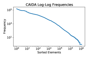
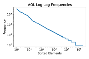
Figure 1: Log-log plots of the sorted frequencies of the first day/minute of the CAIDA/AOL datasets. Both data distributions are heavy-tailed with few items accounting for much of the total stream.

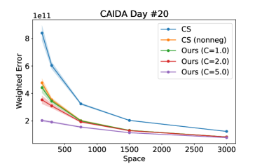
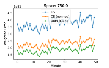
Figure 2: Comparison of weighted error without predictions on the CAIDA dataset. The left plot compares the performance of various algorithms (including our algorithm with different choices of $C$) for a fixed dataset and varying space. The right plot compares algorithms over time across separate streams for each minute of data for a specific choice of space being $750$.

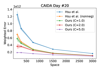
Figure 3: Comparison of weighted error with predictions on the CAIDA dataset.

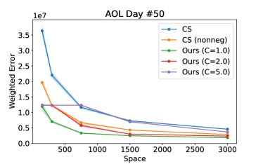
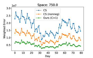
Figure 4: Comparison of weighted error without predictions on the AOL dataset.

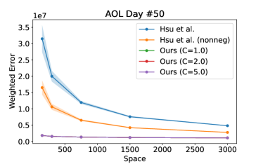
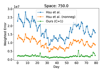
Figure 5: Comparison of weighted error with predictions on the AOL dataset.

Algorithm Implementations

In the setting without predictions, we compare our algorithm to CountSketch (CS) (which was shown to have favorable empirical performance compared to CountMin (CM) in [36] and better theoretical performance due to our work). In the setting with predictions, we compare the algorithm of [36], using CS as the base sketch and dedicated half of the space for items which are predicted to be heavy by the learned oracle. For all implementations, we use three rows in the CS table and vary the number of columns. We additionally augment each of these baselines with a version that truncates all negative estimated frequencies to zero as none of our datasets include stream deletions. This simple change does not change the asymptotic $(\varepsilon,\delta)$ classic sketching guarantees but does make a big difference when measuring empirical weighted error.

We implement a simplified and practical version of our algorithm which uses a single CS table. If the median estimate of an element is below a threshold of $Cn/w$ for domain size $n$, sketch width $w$ (a third of the total space), and a tunable constant $C$, the estimate is instead set to $0$. As all algorithms use a single CS table as the basic building block with different estimation functions, for each trial we randomly sample hash functions for a single CS table and only vary the estimation procedure used.

We evaluate algorithms according the weighted error as in Equation 1 but also according to unweighted error which is simply the sum over all elements of the absolute estimation error, given by $\sum_{i}|f_{i}-\tilde{f}_{i}|$. Space is measured by the size of the sketch table, and all errors are averaged over 10 independent trials with standard deviations shown shaded in.

Datasets

We compare our algorithm with prior work on three datasets. We use the same two real-world datasets and predictions from [36]: the CAIDA and AOL datasets. The CAIDA dataset [12] contains 50 minutes of internet traffic data. For each minute of data, the stream is formed of the IP addresses associated with packets going through a Tier1 ISP. A typical minute of data contains 30 million packets accounted for by 1 million IPs. The AOL dataset [55] contains 80 days of internet search queries with a typical day containing $\approx 3\cdot 10^{5}$ total queries and $\approx 10^{5}$ unique queries. As shown in Figure 1, both datasets approximately follow a power law distribution. For both datasets, we use the predictions from prior work [36] formed using recurrent neural networks. We also generate synthetic data following a Zipfian distribution with $n=10^{7}$ elements and where the $i$th element has frequency $n/i$.

Results

Across the board, our algorithm outperforms the baselines. On the CAIDA and AOL datasets without predictions, our algorithm consistently outperforms the standard CS with up to 4x smaller error with space $300$. This gap widens when we compare our algorithm with predictions to that of [36] with a gap of up to 17x with space $300$. In all cases, the performance of CS and [36] is significantly improved by the simple trick of truncating negative estimates to zero. However, our algorithm still outperforms these “nonneg” baselines. The longitudinal plots which compare algorithms over time show that our algorithm consistently outperforms the state-of-the-art with and without predictions.

In the case of the CAIDA dataset, predictions do not generally improve the performance of any of the algorithms. This is consistent with the findings of [36] where the prediction quality for the CAIDA dataset was relatively poor. However, for the AOL which has a more accurate learned oracle, our algorithm in particular is significantly improved when augmented with predictions. Intuitively, the benefit of our algorithm comes from removing error due to noise for low frequency elements. Conversely, good predictions help to obtain very good estimates of high frequency elements. In combination, this yields very small total weighted error.

In Appendix J, we display comprehensive experiments of the performance of the algorithms across the CAIDA and AOL datasets with varying space and for both weighted and unweighted error as well as results for synthetic Zipfian data. In all cases, our algorithm outperforms the baselines. On synthetic Zipfian, the gap between our algorithm and the non-negative CS for weighted error is relatively small compared to that for the real datasets. While we mainly focus on weighted error in this work, the benefits of our algorithm are even more significant for unweighted error as setting estimates below the noise floor to zero is especially impactful for this error measure. In general, we see the trend, matching our theoretical results, that as space increases, the gap between the different algorithms shrinks as the estimates of the base CS become more accurate.

Appendix A Organization of the Appendix

In Section B, we give tight bounds for CM with Zipfians, as well as tight bounds for CS (in Section C) and its learning augmented variants (in Section D). Our results for CM and CS, with and without predictions, can be summarized in Table 2. We highlight the results of these sections are presented assuming that we use a total of $B$ buckets. With $k$ hash functions, the range of each hash functions is therefore $[B/k]$. We make this assumption since we wish to compare the expected error incurred by the different sketches when the total sketch size is fixed.

Sections E and F contain the proofs of Theorems 2.1 and 3.1, respectively. Section H contains omitted proofs of Section 3.2.

In Section J, we include additional experimental results.

Notation

We use the bracket $[\cdot]$ notation for the indicator function. $a\lesssim b$ denotes $a\leq Cb$ for some fixed positive constant $C$.

	$k=1$	$k>1$
Count-Min (CM)	$\Theta\left(\frac{\log n}{B}\right)$ [36]	$\Theta\left(\frac{k\cdot\log({{kn}\over B})}{B}\right)$
Learned Count-Min (L-CM)	$\Theta\left(\frac{\log^{2}({n\over B})}{B\log n}\right)$ [36]	$\Omega\left(\frac{\log^{2}(\frac{n}{B})}{B\log n}\right)$ [36]
Count-Sketch (CS)	$\Theta\left(\frac{\log B}{B}\right)$	$\Omega\left(\frac{k^{1/2}}{B\log k}\right)$ and $O\left(\frac{k^{1/2}}{B}\right)$
Learned Count-Sketch (L-CS)	$\Theta\left(\frac{\log\frac{n}{B}}{B\log n}\right)$	$\Omega\left(\frac{\log\frac{n}{B}}{B\log n}\right)$

Table 2: This table summarizes our and previously known results on the expected frequency estimation error of Count-Min (CM), Count-Sketch (CS) and their learned variants (i.e., L-CM and L-CS) that use $k$ functions and overall space $k\times{B\over k}$ under Zipfian distribution. For CS, we assume that $k$ is odd (so that the median of $k$ values is well defined).

Appendix B Tight Bounds for Count-Min with Zipfians

For both Count-Min and Count-Sketch we aim at analyzing the expected value of the variable $\sum_{i\in[n]}f_{i}\cdot|\tilde{f}_{i}-f_{i}|$ where $f_{i}=1/i$ and $\tilde{f_{i}}$ is the estimate of $f_{i}$ output by the relevant sketching algorithm. Throughout this paper we use the following notation: For an event $E$ we denote by $[E]$ the random variable in $\{0,1\}$ which is $1$ if and only if $E$ occurs. We begin by presenting our improved analysis of Count-Min with Zipfians. The main theorem is the following.

Theorem B.1.

Let $n,B,k\in\mathbb{N}$ with $k\geq 2$ and $B\leq n/k$. Let further $h_{1},\dots,h_{k}:[n]\to[B]$ be independent and truly random hash functions. For $i\in[n]$ define the random variable $\tilde{f_{i}}=\min_{\ell\in[k]}\left(\sum_{j\in[n]}[h_{\ell}(j)=h_{\ell}(i)]f_{j}\right)$. For any $i\in[n]$ it holds that $\operatorname*{\mathbb{E}}[|\tilde{f}_{i}-f_{i}|]=\Theta\left(\frac{\log\left(\frac{n}{B}\right)}{B}\right)$.

Replacing $B$ by $B/k$ in Theorem B.1 and using linearity of expectation we obtain the desired bound for Count-Min in the upper right hand side of Table 2. The natural assumption that $B\leq n/k$ simply says that the total number of buckets is upper bounded by the number of items.

To prove Theorem B.1 we start with the following lemma which is a special case of the theorem.

Lemma B.2.

Suppose that we are in the setting of Theorem B.1 and further that $n=B$. Then

$$\operatorname*{\mathbb{E}}[|\tilde{f_{i}}-f_{i}|]=O\left(\frac{1}{n}\right).$$

Proof.

It suffices to show the result when $k=2$ since adding more hash functions and corresponding tables only decreases the value of $|\tilde{f}_{i}-f_{i}|$. Define $Z_{\ell}=\sum_{j\in[n]\setminus\{i\}}[h_{\ell}(j)=h_{\ell}(i)]f_{j}$ for $\ell\in[2]$ and note that these variables are independent. For a given $t\geq 3/n$ we wish to upper bound $\Pr[Z_{\ell}\geq t]$. Let $s<t$ be such that $t/s$ is an integer, and note that if $Z_{\ell}\geq t$ then either of the following two events must hold:

1. There exists a $j\in[n]\setminus\{i\}$ with $f_{j}>s$ and $h_{\ell}(j)=h_{\ell}(i)$.

2. The set $\{j\in[n]\setminus\{i\}:h_{\ell}(j)=h_{\ell}(i)\}$ contains at least $t/s$ elements.

To see this, suppose that $Z_{\ell}\geq t$ and that $E_{1}$ does not hold. Then

$$t\leq Z_{\ell}=\sum_{j\in[n]\setminus\{i\}}[h_{\ell}(j)=h_{\ell}(i)]f_{j}\leq s|\{j\in[n]\setminus\{i\}:h_{\ell}(j)=h_{\ell}(i)\}|,$$

so it follows that $E_{2}$ holds. By a union bound,

$$\Pr[Z_{\ell}\geq t]\leq\Pr[E_{1}]+\Pr[E_{2}]\leq\frac{1}{ns}+\binom{n}{t/s}n^{-t/s}\leq\frac{1}{ns}+\left(\frac{es}{t}\right)^{t/s}.$$

Choosing $s=\Theta(\frac{t}{\log(tn)})$ such that $t/s$ is an integer, and using $t\geq{3\over n}$, a simple calculation yields that $\Pr[Z_{\ell}\geq t]=O\left(\frac{\log(tn)}{tn}\right)$. Note that $|\tilde{f_{i}}-f_{i}|=\min(Z_{1},Z_{2})$. As $Z_{1}$ and $Z_{2}$ are independent, $\Pr[|\tilde{f_{i}}-f_{i}|\geq t]=O\left(\left(\frac{\log(tn)}{tn}\right)^{2}\right)$, so

$$\operatorname*{\mathbb{E}}[|\tilde{f_{i}}-f_{i}|]=\int_{0}^{\infty}\Pr[Z\geq t]\,dt\leq\frac{3}{n}+O\left(\int_{3/n}^{\infty}\left(\frac{\log(tn)}{tn}\right)^{2}\,dt\right)=O\left(\frac{1}{n}\right).$$

∎

We can now prove the full statement of Theorem B.1.

Proof of Theorem B.1.

We start out by proving the upper bound. Let $N_{1}=[B]\setminus\{i\}$ and $N_{2}=[n]\setminus([B]\cup\{i\})$. Let $b\in[k]$ be such that $\sum_{j\in N_{1}}f_{j}\cdot[h_{b}(j)=h_{b}(i)]$ is minimal. Note that $b$ is itself a random variable. We also define

$$Y_{1} =\sum_{j\in N_{1}}f_{j}\cdot[h_{b}(j)=h_{b}(i)],\text{ and }Y_{2}=\sum_{j\in N_{2}}f_{j}\cdot[h_{b}(j)=h_{b}(i)].$$

Then, $|\tilde{f}_{i}-f_{i}|\leq Y_{1}+Y_{2}$. Using Lemma B.2, we obtain that $\operatorname*{\mathbb{E}}[Y_{1}]=O(\frac{1}{B})$. For $Y_{2}$ we observe that

$$\operatorname*{\mathbb{E}}[Y_{2}\mid b]=\sum_{j\in N_{2}}\frac{f_{j}}{B}=O\left(\frac{\log\left(\frac{n}{B}\right)}{B}\right).$$

We conclude that

$$\operatorname*{\mathbb{E}}[|\tilde{f}_{i}-f_{i}|]\leq\operatorname*{\mathbb{E}}[Y_{1}]+\operatorname*{\mathbb{E}}[Y_{2}]=\operatorname*{\mathbb{E}}[Y_{1}]+\operatorname*{\mathbb{E}}[\operatorname*{\mathbb{E}}[Y_{2}\mid b]]=O\left(\frac{\log\left(\frac{n}{B}\right)}{B}\right).$$

Next we prove the lower bound. We have already seen that the main contribution to the error comes from the tail of the distribution. As the tail of the distribution is relatively “flat” we can simply apply a concentration inequality to argue that with probability $\Omega(1)$, we have this asymptotic contribution for each of the $k$ hash functions. To be precise, for $j\in[n]$ and $\ell\in[k]$ we define $X_{\ell}^{(j)}=f_{j}\cdot\left([h_{\ell}(j)=h_{\ell}(i)]-\frac{1}{B}\right)$. Note that the variables $(X_{\ell}^{(j)})_{j\in[n]}$ are independent. We also define $S_{\ell}=\sum_{j\in N_{2}}X_{\ell}^{(j)}$ for $\ell\in[k]$. Observe that $|X_{\ell}^{(j)}|\leq f_{j}\leq\frac{1}{B}$ for $j\geq B$, $\operatorname*{\mathbb{E}}[X_{\ell}^{(j)}]=0$, and that

$$\mathrm{Var}[S_{\ell}]=\sum_{j\in N_{2}}f_{j}^{2}\left(\frac{1}{B}-\frac{1}{B^{2}}\right)\leq\frac{1}{B^{2}}.$$

Applying Bennett’s inequality(Theorem I.1 of Appendix I), with $\sigma^{2}=\frac{1}{B^{2}}$ and $M=1/B$ thus gives that

$$\Pr[S_{\ell}\leq-t]\leq\exp\left(-h\left(tB\right)\right).$$

Defining $W_{\ell}=\sum_{j\in N_{2}}f_{j}\cdot[h_{\ell}(j)=h_{\ell}(i)]$ it holds that $\operatorname*{\mathbb{E}}[W_{\ell}]=\Theta\left(\frac{\log\left(\frac{n}{B}\right)}{B}\right)$ and $S_{\ell}=W_{\ell}-\operatorname*{\mathbb{E}}[W_{\ell}]$, so putting $t=\operatorname*{\mathbb{E}}[W_{\ell}]/2$ in the inequality above we obtain that

$$\Pr[W_{\ell}\leq\operatorname*{\mathbb{E}}[W_{\ell}]/2]=\Pr[S_{\ell}\leq-\operatorname*{\mathbb{E}}[W_{\ell}]/2]\leq\exp\left(-h\left(\Omega\left(\log\frac{n}{B}\right)\right)\right).$$

Appealing to Remark I.1 and using that $B\leq n/k$ the above bound becomes

$$\Pr[W_{\ell}\leq\operatorname*{\mathbb{E}}[W_{\ell}]/2] \leq\exp\left(-\Omega\left(\log\frac{n}{B}\cdot\log\left(\log\frac{n}{B}+1\right)\right)\right)$$

$$=\exp(-\Omega(\log k\cdot\log(\log k+1)))=k^{-\Omega(\log(\log k+1))}.$$ (2)

By the independence of the events $(W_{\ell}>E[W_{\ell}]/2)_{\ell\in[k]}$, we have that

$$\Pr\left[|\tilde{f}_{i}-f_{i}|\geq\frac{\operatorname*{\mathbb{E}}[W_{\ell}]}{2}\right]\geq(1-k^{-\Omega(\log(\log k+1))})^{k}=\Omega(1),$$

and so $\operatorname*{\mathbb{E}}[|\tilde{f}_{i}-f_{i}|]=\Omega(\operatorname*{\mathbb{E}}[W_{\ell}])=\Omega\left(\frac{\log\left(\frac{n}{B}\right)}{B}\right)$, as desired. ∎

Remark B.1.

We have stated Theorem B.1 for truly random hash functions but it suffices with $O(\log B)$-independent hashing to prove the upper bound. Indeed, the only step in which we require high independence is in the union bound in Lemma B.2 over the $\binom{n}{t/s}$ subsets of $[n]$ of size $t/s$. To optimize the bound we had to choose $s=t/\log(tn)$, so that $t/s=\log(tn)$. As we only need to consider values of $t$ with $t\leq\sum_{i=1}^{n}f_{i}=O(\log n)$, in fact $t/s=O(\log n)$ in our estimates. Finally, we applied Lemma B.2 with $n=B$ so it follows that $O(\log B)$-independence is enough to obtain our upper bound.

Appendix C (Nearly) Tight Bounds for Count-Sketch with Zipfians

In this section we proceed to analyze Count-Sketch for Zipfians either using a single or more hash functions. We start with two simple lemmas which for certain frequencies $(f_{i})_{i\in[n]}$ of the items in the stream can be used to obtain respectively good upper and lower bounds on $\operatorname*{\mathbb{E}}[|\tilde{f}_{i}-f_{i}|]$ in Count-Sketch with a single hash function. We will use these two lemmas both in our analysis of standard and learned Count-Sketch for Zipfians.

Lemma C.1.

Let $w=(w_{1},\dots,w_{n})\in\mathbb{R}^{n}$, $\eta_{1},\dots,\eta_{n}$ Bernoulli variables taking value $1$ with probability $p$, and $\sigma_{1},\dots,\sigma_{n}\in\{-1,1\}$ independent Rademachers, i.e., $\Pr[\sigma_{i}=1]=\Pr[\sigma_{i}=-1]=1/2$. Let $S=\sum_{i=1}^{n}w_{i}\eta_{i}\sigma_{i}$. Then, $\operatorname*{\mathbb{E}}[|S|]=O\left(\sqrt{p}\|w\|_{2}\right)$.

Proof.

Using that $\operatorname*{\mathbb{E}}[\sigma_{i}\sigma_{j}]=0$ for $i\neq j$ and Jensen’s inequality $\operatorname*{\mathbb{E}}[|S|]^{2}\leq\operatorname*{\mathbb{E}}[S^{2}]=\operatorname*{\mathbb{E}}\left[\sum_{i=1}^{n}w_{i}^{2}\eta_{i}\right]=p\|w\|_{2}^{2}$, from which the result follows. ∎

Lemma C.2.

Suppose that we are in the setting of Lemma C.1. Let $I\subset[n]$ and let $w_{I}\in\mathbb{R}^{n}$ be defined by $(w_{I})_{i}=[i\in I]\cdot w_{i}$. Then

$$\operatorname*{\mathbb{E}}[|S|]\geq\frac{1}{2}p\left(1-p\right)^{|I|-1}\|w_{I}\|_{1}.$$

Proof.

Let $J=[n]\setminus I$, $S_{1}=\sum_{i\in I}w_{i}\eta_{i}\sigma_{i}$, and $S_{2}=\sum_{i\in J}w_{i}\eta_{i}\sigma_{i}$. Let $E$ denote the event that $S_{1}$ and $S_{2}$ have the same sign or $S_{2}=0$. Then $\Pr[E]\geq 1/2$ by symmetry. For $i\in I$ we denote by $A_{i}$ the event that $\{j\in I:\eta_{j}\neq 0\}=\{i\}$. Then $\Pr[A_{i}]=p(1-p)^{|I|-1}$ and furthermore $A_{i}$ and $E$ are independent. If $A_{i}\cap E$ occurs, then $|S|\geq|w_{i}|$ and as the events $(A_{i}\cap E)_{i\in I}$ are disjoint it thus follows that $\operatorname*{\mathbb{E}}[|S|]\geq\sum_{i\in I}\Pr[A_{i}\cap E]\cdot|w_{i}|\geq\frac{1}{2}p\left(1-p\right)^{|I|-1}\|w_{I}\|_{1}$. ∎

With these tools in hand, we proceed to analyse Count-Sketch for Zipfians with one and more hash functions in the next two sections.

C.1 One hash function

By the same argument as in the discussion succeeding Theorem B.1, the following theorem yields the desired result for a single hash function as presented in Table 2.

Theorem C.3.

Suppose that $B\leq n$ and let $h:[n]\to[B]$ and $s:[n]\to\{-1,1\}$ be truly random hash functions. Define the random variable $\tilde{f_{i}}=\sum_{j\in[n]}[h(j)=h(i)]s(j)f_{j}$ for $i\in[n]$. Then

$$\operatorname*{\mathbb{E}}[|\tilde{f}_{i}-s(i)f_{i}|]=\Theta\left(\frac{\log B}{B}\right).$$

Proof.

Let $i\in[n]$ be fixed. We start by defining $N_{1}=[B]\setminus\{i\}$ and $N_{2}=[n]\setminus([B]\cup\{i\})$ and note that

$$|\tilde{f_{i}}-s(i)f_{i}|\leq\left|\sum_{j\in N_{1}}[h(j)=h(i)]s(j)f_{j}\right|+\left|\sum_{j\in N_{2}}[h(j)=h(i)]s(j)f_{j}\right|:=X_{1}+X_{2}.$$

Using the triangle inequality $\operatorname*{\mathbb{E}}[X_{1}]\leq\frac{1}{B}\sum_{j\in N_{1}}f_{j}=O(\frac{\log B}{B})$. Also, by Lemma C.1, $\operatorname*{\mathbb{E}}[X_{2}]=O\left(\frac{1}{B}\right)$ and combining the two bounds we obtain the desired upper bound. For the lower bound we apply Lemma C.2 with $I=N_{1}$ concluding that

$$\operatorname*{\mathbb{E}}[|\tilde{f_{i}}-s(i)f_{i}|]\geq\frac{1}{2B}\left(1-\frac{1}{B}\right)^{|N_{1}|-1}\sum_{i\in N_{1}}f_{i}=\Omega\left(\frac{\log B}{B}\right).$$

∎

C.2 Multiple hash functions

Let $k\in\mathbb{N}$ be odd. For a tuple $x=(x_{1},\dots,x_{k})\in\mathbb{R}^{k}$ we denote by $\operatorname*{\mathsf{median}}x$ the median of the entries of $x$. The following theorem immediately leads to the result on CS with $k\geq 3$ hash functions claimed in Table 2.

Theorem C.4.

Let $k\geq 3$ be odd, $n\geq kB$, and $h_{1},\dots,h_{k}:[n]\to[B]$ and $s_{1},\dots,s_{k}:[n]\to\{-1,1\}$ be truly random hash functions. Define $\tilde{f_{i}}=\operatorname*{\mathsf{median}}_{\ell\in[k]}\left(\sum_{j\in[n]}[h_{\ell}(j)=h_{\ell}(i)]s_{\ell}(j)f_{j}\right)$ for $i\in[n]$. Assume that $k\leq B$. Then

$$\operatorname*{\mathbb{E}}[|\tilde{f_{i}}-s(i)f_{i}|]=\Omega\left(\frac{1}{B\sqrt{k}\log k}\right),\quad\text{and}\quad\operatorname*{\mathbb{E}}[|\tilde{f_{i}}-s(i)f_{i}|]=O\left(\frac{1}{B\sqrt{k}}\right)$$

The assumption $n\geq kB$ simply says that the total number of buckets is upper bounded by the number of items. Again using linearity of expectation for the summation over $i\in[n]$ and replacing $B$ by $B/k$ we obtain the claimed upper and lower bounds of $\frac{\sqrt{k}}{B\log k}$ and $\frac{\sqrt{k}}{B}$ respectively. We note that even if the bounds above are only tight up to a factor of $\log k$ they still imply that it is asymptotically optimal to choose $k=O(1)$, e.g. $k=3$. To settle the correct asymptotic growth is thus of merely theoretical interest.

In proving the upper bound in Theorem C.4, we will use the following result by Minton and Price (Corollary 3.2 of [50]) proved via an elegant application of the Fourier transform.

Lemma C.5 (Minton and Price [50]).

Let $\{X_{i}:i\in[n]\}$ be independent symmetric random variables such that $\Pr[X_{i}=0]\geq 1/2$ for each $i$. Let $X=\sum_{i=1}^{n}X_{i}$ and $\sigma^{2}=\operatorname*{\mathbb{E}}[X^{2}]=\mathrm{Var}[X]$. For $\varepsilon<1$ it holds that $\Pr[|X|<\varepsilon\sigma]=\Omega(\varepsilon)$

Proof of Theorem C.4.

If $B$ (and hence $k$) is a constant, then the results follow easily from Lemma C.1, so in what follows we may assume that $B$ is larger than a sufficiently large constant. We subdivide the exposition into the proofs of the upper and lower bounds.

Upper bound

Define $N_{1}=[B]\setminus\{i\}$ and $N_{2}=[n]\setminus([B]\cup\{i\})$. Let for $\ell\in[k]$, $X_{1}^{(\ell)}=\sum_{j\in N_{1}}[h_{\ell}(j)=h_{\ell}(i)]s_{\ell}(j)f_{j}$ and $X_{2}^{(\ell)}=\sum_{j\in N_{2}}[h_{\ell}(j)=h_{\ell}(i)]s_{\ell}(j)f_{j}$ and let $X^{(\ell)}=X_{1}^{(\ell)}+X_{2}^{(\ell)}$.

As the absolute error in Count-Sketch with one pair of hash functions $(h,s)$ is always upper bounded by the corresponding error in Count-Min with the single hash function $h$, we can use the bound in the proof of Lemma B.2 to conclude that $\Pr[|X_{1}^{(\ell)}|\geq t]=O(\frac{\log(tB)}{tB})$, when $t\geq 3/B$. Also $\mathrm{Var}[X_{2}^{(\ell)}]=(\frac{1}{B}-\frac{1}{B^{2}})\sum_{j\in N_{2}}f_{j}^{2}\leq\frac{1}{B^{2}}$, so by Bennett’s inequality (Theorem I.1) with $M=1/B$ and $\sigma^{2}=1/B^{2}$ and Remark I.1,

$$\Pr[|X_{2}^{(\ell)}|\geq t]\leq 2\exp\left(-h(tB)\right)\leq 2\exp\left(-\frac{1}{2}tB\log\left(tB+1\right)\right)=O\left(\frac{\log(tB)}{tB}\right),$$

for $t\geq\frac{3}{B}$. It follows that for $t\geq 3/B$,

$$\Pr[|X^{(\ell)}|\geq 2t]\leq\Pr[(|X_{1}^{(\ell)}|\geq t)]+\Pr(|X_{2}^{(\ell)}|\geq t)]=O\left(\frac{\log(tB)}{tB}\right).$$

Let $C$ be the implicit constant in the $O$-notation above. If $|\tilde{f_{i}}-s(i)f_{i}|\geq 2t$, at least half of the values $(|X^{(\ell)}|)_{\ell\in[k]}$ are at least $2t$. For $t\geq 3/B$ it thus follows by a union bound that

$$\Pr[|\tilde{f_{i}}-s(i)f_{i}|\geq 2t]\leq 2\binom{k}{\lceil k/2\rceil}\left(C\frac{\log(tB)}{tB}\right)^{\lceil k/2\rceil}\leq 2\left(4C\frac{\log(tB)}{tB}\right)^{\lceil k/2\rceil}.$$ (3)

If $\alpha=O(1)$ is chosen sufficiently large it thus holds that

$$\int_{\alpha/B}^{\infty}\Pr[|\tilde{f_{i}}-s(i)f_{i}|\geq t]\,dt =2\int_{\alpha/(2B)}^{\infty}\Pr[|\tilde{f_{i}}-s(i)f_{i}|\geq 2t]\,dt$$

$$\leq\frac{4}{B}\int_{\alpha/2}^{\infty}\left(4C\frac{\log(t)}{t}\right)^{\lceil k/2\rceil}\,dt$$

$$\leq\frac{1}{B2^{k}}\leq\frac{1}{B\sqrt{k}}.$$

Here the first inequality uses Equation 3 and a change of variable. The second inequality uses that $\left(4C\frac{\log t}{t}\right)^{\lceil k/2\rceil}\leq(C^{\prime}/t)^{2k/5}$ for some constant $C^{\prime}$ followed by a calculation of the integral. Now,

$$\operatorname*{\mathbb{E}}[|\tilde{f_{i}}-s(i)f_{i}|]=\int_{0}^{\infty}\Pr[|\tilde{f_{i}}-s(i)f_{i}|\geq t]\,dt,$$

so for our upper bound it therefore suffices to show that $\int_{0}^{\alpha/B}\Pr[|\tilde{f_{i}}-s(i)f_{i}|\geq t]\,dt=O\left(\frac{1}{B\sqrt{k}}\right)$. For this we need the following claim:

Claim C.6.

Let $I\subset\mathbb{R}$ be the closed interval centered at the origin of length $2t$, i.e., $I=[-t,t]$. Suppose that $0<t\leq\frac{1}{2B}$. For $\ell\in[k]$, $\Pr[X^{(\ell)}\in I]=\Omega(tB)$.

Proof.

Note that $\Pr[X_{1}^{(\ell)}=0]\geq\Pr[\bigwedge_{j\in N_{1}}(h_{\ell}(j)\neq h_{\ell}(i))]=(1-{1\over B})^{N_{1}}=\Omega(1)$. Secondly $\mathrm{Var}[X_{2}^{(\ell)}]=(\frac{1}{B}-\frac{1}{B^{2}})\sum_{j\in N_{2}}f_{j}^{2}\leq\frac{1}{B^{2}}$. Using that $X_{1}^{(\ell)}$ and $X_{2}^{(\ell)}$ are independent and Lemma C.5 with $\sigma^{2}=\mathrm{Var}[X_{2}^{(\ell)}]$, it follows that $\Pr[X^{(\ell)}\in I]=\Omega\left(\Pr[X_{2}^{(\ell)}\in I]\right)=\Omega(tB)$. ∎

Let us now show how to use the claim to establish the desired upper bound. For this let $0<t\leq\frac{1}{2B}$ be fixed. If $|\tilde{f_{i}}-s(i)f_{i}|\geq t$, at least half of the values $(X^{(\ell)})_{\ell\in[k]}$ are at least $t$ or at most $-t$. Let us focus on bounding the probability that at least half are at least $t$, the other bound being symmetric giving an extra factor of $2$ in the probability bound. By symmetry and C.6, $\Pr[X^{(\ell)}\geq t]=\frac{1}{2}-\Omega(tB)$. For $\ell\in[k]$ we define $Y_{\ell}=[X^{(\ell)}\geq t]$, and we put $S=\sum_{\ell\in[k]}Y_{\ell}$. Then $\operatorname*{\mathbb{E}}[S]=k\left(\frac{1}{2}-\Omega(tB)\right)$. If at least half of the values $(X^{(\ell)})_{\ell\in[k]}$ are at least $t$ then $S\geq k/2$. By Hoeffding’s inequality (Theorem I.3) we can bound the probability of this event by

$$\Pr[S\geq k/2]=\Pr[S-\operatorname*{\mathbb{E}}[S]=\Omega(ktB)]=\exp(-\Omega(kt^{2}B^{2})).$$

It follows that $\Pr[|\tilde{f_{i}}-s(i)f_{i}|\geq t]\leq 2\exp(-\Omega(kt^{2}B^{2}))$. Thus

$$\int_{0}^{\alpha/B}\Pr[|\tilde{f_{i}}-s(i)f_{i}|\geq t]\,dt \leq\int_{0}^{\frac{1}{2B}}2\exp(-\Omega(kt^{2}B^{2}))\,dt+\int_{\frac{1}{2B}}^{\alpha/B}2\exp(-\Omega(k))\,dt$$

$$\leq\frac{1}{B\sqrt{k}}\int_{0}^{\sqrt{k}/2}\exp(-t^{2})\,dt+\frac{2\alpha\exp(-\Omega(k))}{B}=O\left(\frac{1}{B\sqrt{k}}\right).$$

Here the second inequality used a change of variable. The proof of the upper bound is complete.

Lower Bound

Fix $\ell\in[k]$ and let $M_{1}=[B\log k]\setminus\{i\}$ and $M_{2}=[n]\setminus([B\log k]\cup\{i\})$. Write

$$S:=\sum_{j\in M_{1}}[h_{\ell}(j)=h_{\ell}(i)]s_{\ell}(j)f_{j}+\sum_{j\in M_{2}}[h_{\ell}(j)=h_{\ell}(i)]s_{\ell}(j)f_{j}:=S_{1}+S_{2}.$$

We also define $J:=\{j\in M_{1}:h_{\ell}(j)=h_{\ell}(i)\}$. Let $I\subseteq\mathbb{R}$ be the closed interval around $s_{\ell}(i)f_{i}$ of length $\frac{1}{B\sqrt{k}\log k}$. We now upper bound the probability that $S\in I$ conditioned on the value of $S_{2}$. To ease the notation, the conditioning on $S_{2}$ has been left out in the notation to follow. Note first that

$$\Pr[S\in I]=\sum_{r=0}^{|M_{1}|}\Pr[S\in I\mid|J|=r]\cdot\Pr[|J|=r].$$ (4)

For a given $r\geq 1$ we now proceed to bound $\Pr[S\in I\mid|J|=r]$. This probability is the same as the probability that $S_{2}+\sum_{j\in R}\sigma_{j}f_{j}\in I$, where $R\subseteq M_{1}$ is a uniformly random $r$-subset and the $\sigma_{j}$’s are independent Rademachers. Suppose that we sample the elements from $R$ as well as the corresponding signs $(\sigma_{i})_{i\in R}$ sequentially, and let us condition on the values and signs of the first $r-1$ sampled elements. At this point at most $\frac{B\log k}{\sqrt{k}}+1$ possible samples for the last element in $R$ can cause that $S\in I$. Indeed, the minimum distance between distinct elements of $\{f_{j}:j\in M_{1}\}$ is at least $1/(B\log k)^{2}$ and furthermore $I$ has length $\frac{1}{B\sqrt{k}\log k}$. Thus, at most

$$\frac{1}{B\sqrt{k}\log k}\cdot(B\log k)^{2}+1=\frac{B\log k}{\sqrt{k}}+1$$

choices for the last element of $R$ ensure that $S\in I$. For $1\leq r\leq(B\log k)/2$ we can thus upper bound

$$\Pr[S\in I\mid|J|=r]\leq\frac{\frac{B\log k}{\sqrt{k}}+1}{|M_{1}|-r+1}\leq\frac{2}{\sqrt{k}}+\frac{2}{B\log k}\leq\frac{3}{\sqrt{k}}.$$

Note that $\mu:=\operatorname*{\mathbb{E}}[|J|]\leq\log k$ so for $B\geq 6$, it holds that

$$\Pr[|J|\geq(B\log k)/2]\leq\Pr\left[|J|\geq\mu\frac{B}{2}\right]\leq\Pr\left[|J|\geq\mu\left(1+\frac{B}{3}\right)\right]\leq\exp\left(-\mu h(B/3)\right)=k^{-\Omega(h(B/3))},$$

where the last inequality follows from the Chernoff bound of Theorem I.2. Thus, if we assume that $B$ is larger than a sufficiently large constant, then $\Pr[|J|\geq B\log k/2]\leq k^{-1}$. Finally, $\Pr[|J|=0]=(1-1/B)^{B\log k}\leq k^{-1}$. Combining the above, we can continue the bound in (4) as follows.

$$\Pr[S\in I]\leq \Pr[|J|=0]+\sum_{r=1}^{(B\log k)/2}\Pr[S\in I\mid|J|=r]\cdot\Pr[|J|=r]$$

$$+ \sum_{r=(B\log k)/2+1}^{|M_{1}|}\Pr[|J|=r]=O\left(\frac{1}{\sqrt{k}}\right),$$ (5)

which holds even after removing the conditioning on $S_{2}$. We now show that with probability $\Omega(1)$ at least half the values $(X^{(\ell)})_{\ell\in[k]}$ are at least $\frac{1}{2B\sqrt{k}\log k}$. Let $p_{0}$ be the probability that $X^{(\ell)}\geq\frac{1}{2B\sqrt{k}\log k}$. This probability does not depend on $\ell\in[k]$ and by symmetry and (5), $p_{0}=1/2-O(1/\sqrt{k})$. Define the function $f:\{0,\dots,k\}\to\mathbb{R}$ by

$$f(t)=\binom{k}{t}p_{0}^{t}(1-p_{0})^{k-t}.$$

Then $f(t)$ is the probability that exactly $t$ of the values $(X^{(\ell)})_{\ell\in[k]}$ are at least $\frac{1}{B\sqrt{k}\log k}$. Using that $p_{0}=1/2-O(1/\sqrt{k})$, a simple application of Stirling’s formula gives that $f(t)=\Theta\left(\frac{1}{\sqrt{k}}\right)$ for $t=\lceil k/2\rceil,\dots,\lceil k/2+\sqrt{k}\rceil$ when $k$ is larger than some constant $C$. It follows that with probability $\Omega(1)$ at least half of the $(X^{(\ell)})_{\ell\in[k]}$ are at least $\frac{1}{B\sqrt{k}\log k}$ and in particular

$$\operatorname*{\mathbb{E}}[|\tilde{f_{i}}-f_{i}|]=\Omega\left(\frac{1}{B\sqrt{k}\log k}\right).$$

Finally we handle the case where $k\leq C$. It follows from simple calculations (e.g., using Lemma C.2) that $X^{(\ell)}=\Omega(1/B)$ with probability $\Omega(1)$. Thus this happens for all $\ell\in[k]$ with probability $\Omega(1)$ and in particular $\operatorname*{\mathbb{E}}[|\tilde{f_{i}}-f_{i}|]=\Omega(1/B)$, which is the desired for constant $k$. ∎

Appendix D Learned Count-Sketch for Zipfians

We now proceed to analyze the learned Count-Sketch algorithm. In Section D.1 we estimate the expected error when using a single hash function and in Section D.2 we show that the expected error only increases when using more hash functions. Recall that we assume that the number of buckets $B_{h}$ used to store the heavy hitters that $B_{h}=\Theta(B-B_{h})=\Theta(B)$.

D.1 One hash function

By taking $B_{1}=B_{h}=\Theta(B)$ and $B_{2}=B-B_{h}=\Theta(B)$ in the theorem below, the result on L-CS for $k=1$ claimed in Table 2 follows immediately.

Theorem D.1.

Let $h:[n]\setminus[B_{1}]\to[B_{2}]$ and $s:[n]\to\{-1,1\}$ be truly random hash functions where $n,B_{1},B_{2}\in\mathbb{N}$ and $n-B_{1}\geq B_{2}\geq B_{1}$. Define the random variable $\tilde{f_{i}}=\sum_{j=B_{1}+1}^{n}[h(j)=h(i)]s(j)f_{j}$ for $i\in[n]\setminus[B_{1}]$. Then

$$\operatorname*{\mathbb{E}}[|\tilde{f}_{i}-s(i)f_{i}|]=\Theta\left(\frac{\log\frac{B_{2}+B_{1}}{B_{1}}}{B_{2}}\right)$$

Proof.

Let $N_{1}=[B_{1}+B_{2}]\setminus([B_{1}]\cup\{i\})$ and $N_{2}=[n]\setminus([B_{1}+B_{2}]\cup\{i\})$. Let $X_{1}=\sum_{j\in N_{1}}[h(j)=h(i)]s(j)f_{j}$ and $X_{2}=\sum_{j\in N_{2}}[h(j)=h(i)]s(j)f_{j}$. By the triangle inequality and linearity of expectation,

$$\operatorname*{\mathbb{E}}[|X_{1}|]=O\left(\frac{\log\frac{B_{2}+B_{1}}{B_{1}}}{B_{2}}\right).$$

Moreover, it follows directly from Lemma C.1 that $\operatorname*{\mathbb{E}}\left[|X_{2}|\right]=O\left(\frac{1}{B_{2}}\right)$. Thus

$$\operatorname*{\mathbb{E}}[|\tilde{f}_{i}-s(i)f_{i}|]\leq\operatorname*{\mathbb{E}}[|X_{1}|]+\operatorname*{\mathbb{E}}[|X_{2}|]=O\left(\frac{\log\frac{B_{2}+B_{1}}{B_{1}}}{B_{2}}\right),$$

as desired. For the lower bound on $\operatorname*{\mathbb{E}}\left[\left|\tilde{f_{i}}-s(i)f_{i}\right|\right]$ we apply Lemma C.2 with $I=N_{1}$ to obtain that,

$$\operatorname*{\mathbb{E}}\left[\left|\tilde{f_{i}}-s(i)f_{i}\right|\right]\geq\frac{1}{2B_{2}}\left(1-\frac{1}{B_{2}}\right)^{|N_{1}|-1}\sum_{i\in N_{1}}f_{i}=\Omega\left(\frac{\log\frac{B_{2}+B_{1}}{B_{1}}}{B_{2}}\right).$$

∎

Corollary D.2.

Let $h:[n]\setminus[B_{h}]\to[B-B_{h}]$ and $s:[n]\to\{-1,1\}$ be truly random hash functions where $n,B,B_{h}\in\mathbb{N}$ and $B_{h}=\Theta(B)\leq B/2$. Define the random variable $\tilde{f_{i}}=\sum_{j=B_{h}+1}^{n}[h(j)=h(i)]s(j)f_{j}$ for $i\in[n]\setminus[B_{h}]$. Then $\operatorname*{\mathbb{E}}[|\tilde{f}_{i}-s(i)f_{i}|]=\Theta(1/B)$.

Remark D.1.

The upper bounds of Theorem D.1 and Corollary D.2 hold even without the assumption of fully random hashing. In fact, we only require that $h$ and $s$ are $2$-independent. Indeed Lemma C.1 holds even when the Rademachers are $2$-independent (the proof is the same). Moreover, we need $h$ to be $2$-independent as we condition on $h(i)$ in our application of Lemma C.1. With $2$-independence the variables $[h(j)=h(i)]$ for $j\neq i$ are then Bernoulli variables taking value $1$ with probability $1/B_{2}$.

D.2 More hash functions

We now show that, like for Count-Sketch, using more hash functions does not decrease the expected error. We first state the Littlewood-Offord lemma as strengthened by Erdős.

Theorem D.3 (Littlewood-Offord [45], Erdős [29]).

Let $a_{1},\dots,a_{n}\in\mathbb{R}$ with $|a_{i}|\geq 1$ for $i\in[n]$. Let further $\sigma_{1},\dots,\sigma_{n}\in\{-1,1\}$ be random variables with $\Pr[\sigma_{i}=1]=\Pr[\sigma_{i}=-1]=1/2$ and define $S=\sum_{i=1}^{n}\sigma_{i}a_{i}$. For any $v\in\mathbb{R}$ it holds that $\Pr[|S-v|\leq 1]=O(1/\sqrt{n})$.

Setting $B_{1}=B_{h}=\Theta(B)$ and $B_{2}=B-B_{2}=\Theta(B)$ in the theorem below gives the final bound from Table 2 on L-CS with $k\geq 3$.

Theorem D.4.

Let $n\geq B_{1}+B_{2}\geq 2B_{1}$, $k\geq 3$ odd, and $h_{1},\dots,h_{k}:[n]\setminus[B_{1}]\to[B_{2}/k]$ and $s_{1},\dots,s_{k}:[n]\setminus[B_{1}]\to\{-1,1\}$ be independent and truly random. Define the random variable $\tilde{f_{i}}=\operatorname*{\mathsf{median}}_{\ell\in[k]}\left(\sum_{j\in[n]\setminus[B_{1}]}[h_{\ell}(j)=h_{\ell}(i)]s_{\ell}(j)f_{j}\right)$ for $i\in[n]\setminus[B_{1}]$. Then

$$\operatorname*{\mathbb{E}}[|\tilde{f}_{i}-s(i)f_{i}|]=\Omega\left(\frac{1}{B_{2}}\right).$$

Proof.

Like in the proof of the lower bound of Theorem C.4 it suffices to show that for each $i$ the probability that the sum $S_{\ell}:=\sum_{j\in[n]\setminus([B_{1}]\cup\{i\})}[h_{\ell}(j)=h_{\ell}(i)]s_{\ell}(j)f_{j}$ lies in the interval $I=\left[-1/(2B_{2}),1/(2B_{2})\right]$ is $O(1/\sqrt{k})$. Then at least half the $(S_{\ell})_{\ell\in[k]}$ are at least $1/(2B_{2})$ with probability $\Omega(1)$ by an application of Stirling’s formula, and it follows that $\operatorname*{\mathbb{E}}[|\tilde{f}_{i}-s(i)f_{i}|]=\Omega(1/B_{2})$.

Let $\ell\in[k]$ be fixed, $N_{1}=[2B_{2}]\setminus([B_{2}]\cup\{i\})$, and $N_{2}=[n]\setminus(N_{1}\cup\{i\})$, and write

$$S_{\ell}=\sum_{j\in N_{1}}[h_{\ell}(j)=h_{\ell}(i)]s_{\ell}(j)f_{j}+\sum_{j\in N_{2}}[h_{\ell}(j)=h_{\ell}(i)]s_{\ell}(j)f_{j}:=X_{1}+X_{2}.$$

Now condition on the value of $X_{2}$. Letting $J=\{j\in N_{1}:h_{\ell}(j)=h_{\ell}(i)\}$ it follows by Theorem D.3 that

$$\Pr[S_{\ell}\in I\mid X_{2}]=O\left(\sum_{J^{\prime}\subseteq N_{1}}\frac{\Pr[J=J^{\prime}]}{\sqrt{|J^{\prime}|+1}}\right)=O\left(\Pr[|J|<k/2]+1/\sqrt{k}\right).$$

An application of Chebyshev’s inequality gives that $\Pr[|J|<k/2]=O(1/k)$, so $\Pr[S_{\ell}\in I]=O(1/\sqrt{k})$. Since this bound holds for any possible value of $X_{2}$ we may remove the conditioning and the desired result follows. ∎

Remark D.2.

The bound above is probably only tight for $B_{1}=\Theta(B_{2})$. Indeed, we know that it cannot be tight for all $B_{1}\leq B_{2}$ since when $B_{1}$ becomes very small, the bound from the standard Count-Sketch with $k\geq 3$ takes over — and this is certainly worse than the bound in the theorem. It is an interesting open problem (that requires a better anti-concentration inequality than the Littlewood-Offord lemma) to settle the correct bound when $B_{1}\ll B_{2}$.

Appendix E Proof of Theorem 2.1

In this section we give the complete proof of Theorem 2.1. We need the following special case of a result about the behaviour of CountSketch, proved in the prior sections.

Theorem E.1 (Theorem C.4).

Let $\hat{f}_{i}$ be the estimate of the $i$th frequency given by a $3\times B/3$ CountSketch table. There exists a universal constant $C$ such that the following two inequalities hold:

$$\Pr\left(|f_{i}-\hat{f}_{i}^{j}|\geq\frac{C}{B}\right) \leq\frac{1}{2},$$ (6)

$$\forall t\geq 3/B,\quad\Pr\left(|f_{i}-\hat{f}_{i}^{j}|\geq t\right) \leq C\left(\frac{\log(tB)}{tB}\right)^{2}.$$ (7)

Proof of Theorem 2.1.

Case 1: $i>B/\log\log n$. Recall that $\hat{f}_{i}^{j}$ denotes the estimate of the $i$th frequency given by table $S_{j}$ in Algorithm 2. Furthermore, $\tilde{f}_{i}\leftarrow\text{Median}(\hat{f}_{i}^{1},\ldots,\hat{f}_{i}^{T-1})$ denotes the median of the estimates of the first $T-1$ tables in Algorithm 2. From Theorem E.1, we have that for every fixed $j$,

$$\Pr\left(|f_{i}-\hat{f}_{i}^{j}|\geq\frac{2C\log\log n}{B}\right)\leq\frac{1}{4}$$

and so it follows that

$$\Pr\left(|f_{i}-\tilde{f}_{i}|\geq\frac{2C\log\log n}{B}\right)\leq\exp(-\Omega(T))\leq\frac{1}{(\log n)^{100}}$$ (8)

by adjusting the constant in front of $T$. We let $2C$ be the constant for the $O$ notation in line $7$ of Algorithm 2. Now consider the expected value of $|\hat{f}_{i}-1/i|$, where the expectation is taken over the randomness used by the CountSketch tables of Algorithm 2. By conditioning on the event that we either output $0$ or output the estimate of the $T$th table, we have

$$\mathbb{E}\left[\frac{1}{i}\cdot\left|\hat{f}_{i}-\frac{1}{i}\right|\right]\lesssim\Pr(\text{We output $0$})\cdot\frac{1}{i^{2}}+\Pr(\text{We output estimate of table $T$})\cdot\frac{1}{iB}$$

where we have used the first inequality in Theorem E.1 in the above inequality and $\lesssim$ denotes inequality up to a constant factor. We have bounded the second probability in Equation (8) which gives

$$\mathbb{E}\left[\frac{1}{i}\cdot\left|\hat{f}_{i}-\frac{1}{i}\right|\right]\lesssim\frac{1}{i^{2}}+\frac{1}{iB\cdot(\log n)^{99}}.$$ (9)

Case 2: $i\leq B/(\log\log n)^{4}$. We employ the more refined tail bound for Count Sketch stated in the second inequality of Theorem E.1.

For any $i$ smaller than $B/(\log\log n)^{4}$, we have that for any fixed $j$,

$$\Pr\left(\hat{f}_{i}^{j}\leq\frac{2C\log\log n}{B}\right)\leq\Pr\left(|f_{i}-\hat{f}_{i}^{j}|\geq\frac{1}{2i}\right)\lesssim\left(\frac{\log(B^{\prime}/i)\cdot i}{B^{\prime}}\right)^{2}$$

where $B^{\prime}=B/(4T)=\Theta(B/\log\log n)$. It follows that

$$\Pr\left(\tilde{f}_{i}\leq\frac{2C\log\log n}{B}\right)\leq T\cdot\Pr\left(|f_{i}-\hat{f}_{i}^{1}|\leq\frac{2C\log\log n}{B}\right)\lesssim T\cdot\left(\frac{\log(B^{\prime}/i)\cdot i}{B^{\prime}}\right)^{2}.$$

Therefore, for $i\leq B/(\log\log n)^{4}$, we again have

$$\mathbb{E}\left[\frac{1}{i}\cdot\left|\hat{f}_{i}-\frac{1}{i}\right|\right] \lesssim\Pr(\text{We output $0$})\cdot\frac{1}{i^{2}}+\Pr(\text{We output estimate of table $T$})\cdot\frac{1}{iB}$$

$$\lesssim(\log\log n)^{3}\cdot\left(\frac{\log(B/i)}{B}\right)^{2}+\frac{1}{iB}.$$

We can summarize this case as:

$$\mathbb{E}\left[\frac{1}{i}\cdot\left|\hat{f}_{i}-\frac{1}{i}\right|\right]\lesssim(\log\log n)^{3}\cdot\left(\frac{\log(B/i)}{B}\right)^{2}+\frac{1}{iB}.$$ (10)

Putting everything together. Equation (9) gives us

$$\frac{1}{\log n}\cdot\sum_{i>B/\log\log n}\mathbb{E}\left[\frac{1}{i}\cdot\left|\hat{f}_{i}-\frac{1}{i}\right|\right] \lesssim\frac{1}{\log n}\sum_{i>B/\log\log n}\frac{1}{i^{2}}+\frac{1}{B\cdot(\log n)^{100}}\,\sum_{i=1}^{n}\frac{1}{i}$$

$$\lesssim\frac{\log\log n}{B\log n}.$$

Equation (10) gives us

$$\frac{1}{\log n}\cdot\sum_{i\leq B/(\log\log n)^{4}}\mathbb{E}\left[\frac{1}{i}\cdot\left|\hat{f}_{i}-\frac{1}{i}\right|\right] \lesssim\frac{1}{\log n}\sum_{i\leq B/(\log\log n)^{4}}\left((\log\log n)^{3}\cdot\left(\frac{\log(B/i)}{B}\right)^{2}+\frac{1}{iB}\right)$$

$$\lesssim\frac{(\log\log n)^{3}}{B^{2}\log n}\int_{1}^{B/(\log\log n)^{4}}\log(B/x)^{2}\ dx+\frac{\log B}{B\log n}$$

$$\lesssim\frac{(\log\log n)^{3}}{B^{2}\log n}\cdot\frac{B(\log^{2}(\log\log n))}{(\log\log n)^{4}}+\frac{\log B}{B\log n}$$

$$\lesssim\frac{\log B}{B\log n}$$

where the second to last inequality follows from the indefinte integral $\int\log^{2}(c/x)\ dx=x\log^{2}(c/x)+2x\log(c/x)+2x+\text{Constant}$.

Finally, we deal with the remaining case: $i$ between $B/\log\log n$ and $B/(\log\log n)^{4}$. For these $i$’s, the worst case error happens when we set their estimates to $0$, incurring error $1/i$, as opposed to incurring error $O(1/B)$ if we used the estimate of table $T$:

$$\frac{1}{\log n}\cdot\sum_{B/(\log\log n)^{4}\leq i\leq B/\log\log n}\mathbb{E}\left[\frac{1}{i}\cdot\left|\hat{f}_{i}-\frac{1}{i}\right|\right]$$

$$\lesssim\frac{1}{\log n}\sum_{B/(\log\log n)^{4}\leq i\leq B/\log\log n}\frac{1}{i^{2}}$$

$$\lesssim\frac{(\log\log n)^{4}}{B\log n}.$$

Combining our three estimates completes the proof. ∎

Appendix F Proof of Theorem 3.1

Proof of Theorem 3.1.

We summarize the intuition and give the full proof. Recall the workhorse of our analysis is the proof of Theorem 2.1. First note that we obtain $0$ error for $i<B/2$. Thus, all our error comes from indices $i\geq B/2$. Recall the intuition for this case from the proof of Theorem 2.1: we want to output $0$ as our estimates. Now the same analysis as in Case $1$ of Theorem 2.1 gives us that the probability we use the estimate of table $T$ can be bounded by say $\frac{1}{(\log n)^{100}}$. Thus, similar to Equation (9), we have

$$\mathbb{E}\left[\frac{1}{i}\cdot\left|\hat{f}_{i}-\frac{1}{i}\right|\right] \lesssim\Pr(\text{We output $0$})\cdot\frac{1}{i^{2}}+\Pr(\text{We output estimate of table $T$})\cdot\frac{1}{iB}$$

$$\lesssim\frac{1}{i^{2}}+\frac{1}{iB\cdot(\log n)^{99}}.$$

Thus, our total error consists of only one part of the total error calculation of Theorem 2.1:

$$\frac{1}{\log n}\cdot\sum_{i>B}\mathbb{E}\left[\frac{1}{i}\cdot\left|\hat{f}_{i}-\frac{1}{i}\right|\right] \lesssim\frac{1}{\log n}\sum_{i>B}\frac{1}{i^{2}}+\frac{1}{B\cdot(\log n)^{100}}\,\sum_{i=1}^{n}\frac{1}{i}$$

$$\lesssim\frac{1}{B\log n},$$

as desired. ∎

Algorithm 5 Parsimonious frequency update algorithm

1:Input: Stream of updates to an $n$ dimensional vector, space budget $B$, access to a heavy hitter oracle which correctly identifies the top $B/2$ heavy hitters.

2:procedure Update

3:     $T\leftarrow O(\log\log n)$

4:     for $j=1$ to $T-1$ do

5:         $S_{j}\leftarrow$ CountSketch table with $4$ rows and $\frac{B}{16T}$ columns

6:     end for

7:     $S_{T}\leftarrow$ CountSketch table with $4$ rows and $\frac{B}{16}$ columns

8:     for stream element $(i,\Delta)$ do

9:         if $i$ is already classified as a top $B/2$ heavy hitter then

10:              Maintain the count of $i$ exactly (from the point of time it was detected as heavy).

11:         else

12:              Query the heavy hitter oracle with probability $p=\min\left(1,CB(\log n)^{2}\Delta\right)$

13:              if $i$ gets queried and is classified as a top $B/2$ heavy hitter then

14:                  Maintain the count of $i$ exactly (from this point of time).

15:              else

16:                  Input $(i,\Delta)$ in each of the $T$ CountSketch tables $S_{j}$

17:              end if

18:         end if

19:     end for

20:end procedure

Appendix G Parsimonious learning

In this appendix, we state our result on parsimonious learning precisely. We consider the modification to Algorithm 3 where whenever an element $(i,\Delta)$ arrives, we only query the heavy hitter oracle with probability $p=\min\left(1,\gamma B(\log n)^{2}\Delta\right)$ for $\gamma$ a sufficiently large constant. To be precise, when an item $i$ arrives, we first check if it is already classified as a top $B/2$ heavy hitter. If so, we update its exact count (from the first point of time where it was classified as heavy). If not, we query the heavy hitter oracle with probability $p$. In case $i$ gets queried and classified as one of the top $B/2$ heavy hitters, we store its count exactly (from this point of time). Otherwise, we input it to the CountSketch tables $S_{j}$ similarly to Algorithm 1 and Algorithm 3. Algorithm 5 shows the pseudocode for the update procedure of our parsimonious learning algorithm. The query procedure is similar to Algorithm 4. We now state our main result on our parsimonious learning algorithm, namely that it achieves the same expected weighted error bound as in Theorem 3.1.

Theorem G.1.

Consider Algorithm 5 with space parameter $B\geq\log n$ updated over a Zipfian stream. Suppose the heavy-hitter oracle correctly identifies the top $B/2$ heavy hitters in the stream. Let $\{\hat{f}_{i}\}_{i=1}^{n}$ denote the estimates computed by Algorithm 4. The expected weighted error (1) is $\mathbb{E}\left[\frac{1}{N}\cdot\sum_{i=1}^{n}f_{i}\cdot|f_{i}-\hat{f}_{i}|\right]=O\left(\frac{1}{B\log n}\right).$ The algorithm makes $O(B(\log n)^{3})$ queries to the heavy hitter oracle in expectation.

Proof of Theorem G.1.

Introducing some notation, we denote the stream $((x_{1},\Delta_{1}),\dots,(x_{m},\Delta_{m}))$. Letting $S_{i}=\{j\in[m]\mid x_{j}=i\}$, we then have that $\sum_{j\in S_{i}}\Delta_{j}=f_{j}=1/j$. Then, whenever an element $(x_{j},\Delta_{j})$ arrives, the algorithm queries the heavy hitter oracle with probability $p_{j}=\min\left(1,C\gamma B(\log n)^{2}\Delta_{j}\right)$.

Let us first consider the expected error when estimating the frequency of a heavy hitter $i\leq B/2$. Let $j_{0}\in S_{i}$ be minimal such that $\sum_{j\in S_{i},j\leq j_{0}}\Delta_{j}\geq\frac{1}{B\log n}$. Since $i$ is a heavy hitter with total frequency $f_{i}\geq 2/B$, such a $j_{0}$ exists. If there exists $j\in S_{i}$ with $j\leq j_{0}$ such that $p_{j}=1$, then $i$ will be classified as a heavy hitter by time $j_{0}$ with probability $1$. Otherwise, the probability that $i$ is not classified as a heavy hitter by time $j_{0}$ is upper bounded by

$$\prod_{j\in S_{i},j\leq j_{0}}(1-p_{j})\leq \exp\left(-\sum_{j\in S_{i},j\leq j_{0}}p_{j}\right)=\exp\left(-\gamma B(\log n)^{2}\sum_{j\in S_{i},j\leq j_{0}}\Delta_{j}\right)$$

$$\leq \exp(-\gamma\log n)=n^{-\gamma}.$$

Union bounding over the $B/2$ top heavy hitters we find that with high probability in $n$ they are indeed classified as heavy at the first point of time where they have appeared with weight at least $\frac{1}{B\log n}$. In particular, with the same high probability the error when estimating each of the top $B/2$ heavy hitters is at most $\frac{1}{B\log n}$ and so,

$$\mathbb{E}\left[\frac{1}{N}\cdot\sum_{i=1}^{B/2}f_{i}\cdot|f_{i}-\hat{f}_{i}|\right]=O\left(\frac{1}{B\log n}\right).$$

Let us now consider the light elements $i>B/2$. Such an element is never classified as heavy and consequently is estimated using the CountSketch tables $S_{j}$ as in Algorithm 2. Denoting by $E$ the event that we output $0$ (that is, the median of the first $T-1$ CountSketch tables is small enough) and by $E^{c}$ the event that we output the estimate from table $T$, as in Appendix F, we again have

$$\mathbb{E}\left[\frac{1}{i}\cdot\left|\hat{f}_{i}-\frac{1}{i}\right|\right]\lesssim\Pr(E)\cdot\frac{1}{i^{2}}+\Pr(E^{c})\cdot\frac{1}{iB}\leq\frac{1}{i^{2}}+\Pr(E^{c})\cdot\frac{1}{iB}.$$

Here, the bound of $O(1/B)$ on the expected error of table $T$ holds even though the $B/2$ heavy hitters might appear in table $T$. The reason is with high probability, these heavy hitters appear with weight at most $\frac{1}{B\log n}$ and conditioned on this event, we can plug into Lemma C.1 to get that the expected error is still $O(1/B)$. It remains to bound $\Pr(E^{c})$. Again, from Lemma C.1, it follows that the expected error of each of the first $T-1$ tables is at most $C\frac{2\log\log n}{B}$ for a sufficiently large constant $C$ (even including the contribution from the heavy hitters), and so by Markov’s inequality,

$$\Pr\left(|f_{i}-\hat{f}_{i}^{j}|\geq\frac{2C\log\log n}{B}\right)\leq\frac{1}{4}$$

and again,

$$\Pr\left(|f_{i}-\tilde{f}_{i}|\geq\frac{2C\log\log n}{B}\right)\leq\exp(-\Omega(T))\leq\frac{1}{(\log n)^{100}}.$$

Thus, we can bound,

$$\mathbb{E}\left[\frac{1}{i}\cdot\left|\hat{f}_{i}-\frac{1}{i}\right|\right]\lesssim\frac{1}{i^{2}}+\cdot\frac{1}{(\log n)^{100}iB}.$$

Recalling that $N=H_{n}$ and summing over $i\geq B/2$ we get that

$$\mathbb{E}\left[\frac{1}{N}\cdot\sum_{i=B/2+1}^{n}f_{i}\cdot|f_{i}-\hat{f}_{i}|\right]=O\left(\frac{1}{B\log n}+\frac{\log(n/B)}{B(\log n)^{100}}\right)=O\left(\frac{1}{B\log n}\right),$$

as desired. The expected number of queries to the heavy hitter oracle is

$$\sum_{j=1}^{m}p_{j}\leq\sum_{i=1}^{n}\sum_{j\in S_{i}}\gamma B(\log n)^{2}\Delta_{j}=\sum_{i=1}^{n}\gamma B(\log n)^{2}f_{i}=O(B(\log n)^{3}).$$

Remark G.1.

We note that Algorithm 5 makes use of the length of the stream to set $p$. Usually we would not know the length of the stream but at the cost of an extra log-factor in the number of queries made to the oracle, we can remedy this. Indeed, the query probability is $p=\min\left(1,\frac{\gamma B(\log n)^{3}}{m}\right)$ where $m$ is the length of the stream. If we instead increase the query probability after we have seen $j$ stream elements to $p_{j}=\min\left(1,\frac{\gamma B(\log n)^{3}}{j}\right)$, we obtain the same bound on the expected weighted error. Indeed, we will only detect the heavy hitters earlier. Moreover, the expected number of queries to the oracle is at most

$$\sum_{j=1}^{m}\frac{\gamma B(\log n)^{3}}{j}=O\left(B(\log n)^{3}\log m\right).$$

∎

Appendix H Omitted Proofs of Section 3.2

In this section, we discuss a version of our algorithm using a worst case estimate of the tail of the distribution, generalizing the value $O(AT/B)$ designed for Zipfian distributions. The algorithm Basic-Tail-Sketch is essentially the classic AMS sketch [2] with $c=O(1)$ counters for the elements whose hash value is $1$. It is easy to see that the final algorithm, Algorithm 6 uses $O(B)$ words of space.

Algorithm 6 Estimating the tail of the frequency vector $f$

1:Input: Stream of updates to an $n$ dimensional vector $f$, space budget $O(B)$

2:procedure Tail-Estimator

3:     Initialize $B$ independent copies of Basic-Tail-Sketch

4:     Update each copy of Basic-Tail-Sketch with updates from the stream

5:     for $1\leq i\leq B$ do

6:         $V_{i}\leftarrow$ value outputted by $i$th copy of Basic-Tail-Sketch after stream ends

7:     end for

8:     Return $V\leftarrow$ the $B/3$-th largest value among $\{V_{i}\}_{i=1}^{B}$

9:end procedure

Algorithm 7 Auxilliary algorithm for Algorithm 6

1:Input: Stream of updates to an $n$ dimensional vector $f$

2:procedure Basic-Tail-Sketch

3:     $T\leftarrow\Theta(\log\log n)$

4:     $B^{\prime}\leftarrow\Theta(B/T)$

5:     $h:[n]\rightarrow[B^{\prime}]$ (4-wise independent hash function)

6:     $c\leftarrow 32$

7:     for $1\leq j\leq c$ do

8:         $s_{j}:[n]\rightarrow\{\pm 1\}$ (4-wise independent hash function)

9:     end for

10:     Keep track of the sum $\frac{1}{c}\sum_{j=1}^{c}\left(\sum_{i:h(i)=1}f_{i}s_{j}(i)\right)^{2}$

11:end procedure

We now show that $V$, the output of Algorithm 6, satisfies $V\approx\|f_{\overline{\Theta(B^{\prime})}}\|_{2}^{2}/B^{\prime}$, which is of the same order as the threshold value used in line $7$ of Algorithm 4, generalizing the Zipfian case.

Proof of Lemma 3.2.

We analyze one copy of the sketch $V_{1}$, starting with the upper bound.

Let $a$ be the number of elements $i\in[B^{\prime}/10]$ such that $h(i)=1$. Because $\operatorname*{\mathbb{E}}[a]=1/10$, by Markov’s inequality, we have $a\leq 9/10$ with probability at least $8/9$. Next, let $W_{j}=\sum_{i>B^{\prime}/10:h(i)=1}f_{i}s_{j}(i)$. We have

$$\operatorname*{\mathbb{E}}[W_{j}^{2}]=\sum_{i\geq B^{\prime}/10}f_{i}^{2}\cdot[h(i)=1]=\left\|f_{\overline{B^{\prime}/10}}\right\|_{2}^{2}/B^{\prime}$$

By Markov’s inequality, we have $\frac{1}{4}\sum_{j}W_{j}^{2}\leq 9\left\|f_{\overline{B^{\prime}/10}}\right\|_{2}^{2}/B^{\prime}$ with probability $8/9$. By the union bound, $V_{1}^{2}\leq 9\left\|f_{\overline{B^{\prime}/10}}\right\|_{2}^{2}/B$ with probability at least $7/9$.

Next, we show the lower bound. Let $X_{1}=\sum_{i:h(i)=1}\min\left(f_{i}^{2},f_{3B^{\prime}}^{2}\right)$ and $Y_{1}=\sum_{i:h(i)=1}f_{i}^{2}$. Observe that $X_{1}\leq Y_{1}$. We have

$$\operatorname*{\mathbb{E}}_{h}\left[X_{1}\right] =\left\|f_{\overline{3B^{\prime}}}\right\|_{2}^{2}/B^{\prime}+3f_{3B^{\prime}}^{2}$$

$$Var\left(X_{1}\right) =\frac{B^{\prime}-1}{B^{\prime 2}}\left(\sum_{i>3B^{\prime}}f_{i}^{4}+3Bf_{3B^{\prime}}^{4}\right)$$

By Chebyshev’s inequality,

$$\Pr\left[X_{1}\leq\left\|f_{\overline{3B^{\prime}}}\right\|_{2}^{2}/(3B^{\prime})\right] \leq\frac{\frac{B^{\prime}-1}{B^{\prime 2}}\left(\sum_{i>3B^{\prime}}f_{i}^{4}+3B^{\prime}f_{3B^{\prime}}^{4}\right)}{\left(2\left\|f_{\overline{3B^{\prime}}}\right\|_{2}^{2}/(3B^{\prime})+3f_{3B^{\prime}}^{2}\right)^{2}}$$

$$\leq\frac{\left(B^{\prime}-1\right)\left(\sum_{i>3B}f_{i}^{4}+3B^{\prime}f_{3B^{\prime}}^{4}\right)}{4\left\|f_{\overline{3B^{\prime}}}\right\|_{2}^{4}/9+9B^{\prime 2}f_{3B^{\prime}}^{2}+4B^{\prime}\left\|f_{\overline{3B^{\prime}}}\right\|_{2}^{2}f_{3B^{\prime}}^{2}}$$

$$\leq\frac{1}{3}.$$

Thus, with probability at least $2/3$, we have $Y_{1}\geq\left\|f_{\overline{3B^{\prime}}}\right\|_{2}^{2}/(3B^{\prime})$. Next we can bound $V_{1}$ in terms of $Y_{1}$ using the standard analysis of the AMS sketch. Let $Z_{j}=\sum_{i:h(i)=1}f_{i}s_{j}(i)$.

$$\operatorname*{\mathbb{E}}_{s}\left[Z_{j}^{2}|h\right] =Y_{1}$$

$$\operatorname*{\mathbb{E}}_{s}\left[Z_{j}^{4}|h\right] =\sum_{i:h(i)=1}f_{i}^{4}+6\sum_{i<j:h(i)=h(j)=1}f_{i}^{2}f_{j}^{2}=3Y_{1}^{2}-2\sum_{i:h(i)=1}f_{i}^{4}.$$

By the Chebyshev’s inequality, $\Pr\left[V_{1}\leq Y_{1}/2\right]\leq\frac{2Y_{1}^{2}/c}{Y_{1}^{2}/4}\leq\frac{8}{c}\leq\frac{1}{4}$. By the union bound, we have $V_{1}\geq\left\|f_{\overline{3B}}\right\|_{2}^{2}/(6B^{\prime})$ with probability at least $5/12$.

The lemma follows from applying the Chernoff bound to the independent copies $V_{1},\ldots,V_{B}$. ∎

Given the estimator $V$, we can output $0$ for elements whose squared estimated frequency is below $V$.

Lemma H.1.

Let $E$ be the event that $V$ is accurate, which holds with probability $1-\exp\left(\Omega\left(B\right)\right)$. If $f_{i}^{2}\leq\left\|f_{\overline{3B^{\prime}}}\right\|_{2}^{2}/(12B^{\prime})$ then with probability $1-\exp\left(\Omega\left(B\right)\right)-1/polylog(n)$, the algorithm outputs $0$. If $f_{i}^{2}\geq\left\|f_{\overline{3B^{\prime}}}\right\|_{2}^{2}/(12B^{\prime})$ then with constant probability,

$$\left\|f_{i}^{2}-\hat{f}_{i}^{2}\right\|\leq O\left(\left\|f_{\overline{\Omega(B^{\prime})}}\right\|_{2}^{2}/B^{\prime}\right)$$

Proof.

Observe that the error in the comparison between the threshold $V$ and $\tilde{f}_{i}$ is bounded by $V$ plus the estimation error of $\tilde{f}_{i}$. By the standard analysis of the CountSketch, with probability $1-\exp\left(\Omega\left(T\right)\right)$,

$$\left|f_{i}^{2}-\tilde{f}_{i}^{2}\right|\leq O\left(\left\|f_{\overline{\Omega(B^{\prime})}}\right\|_{2}^{2}/B^{\prime}\right)$$

Thus, if $f_{i}^{2}\leq\left\|f_{\overline{3B^{\prime}}}\right\|_{2}^{2}/(12B^{\prime})$ then with probability $1-\exp\left(\Omega\left(B\right)\right)-1/polylog(n)$, we have $V\geq\tilde{f}_{i}$ and the algorithm outputs $0$.

On the other hand, consider $f_{i}^{2}\geq\left\|f_{\overline{3B^{\prime}}}\right\|_{2}^{2}/(12B^{\prime})$. First, consider the case when the algorithm outputs $0$. Except for a failure probability of $\exp\left(\Omega\left(B\right)\right)+1/polylog(n)$, it must be the case that $f_{i}^{2}=O\left(\left\|f_{\overline{3B^{\prime}}}\right\|_{2}^{2}/(12B^{\prime})\right)$ so we have $|f_{i}^{2}-0|=O\left(\left\|f_{\overline{3B^{\prime}}}\right\|_{2}^{2}/(12B^{\prime})\right)$. Next, consider the case when the algorithm outputs the answer from $S_{T}$. The correctness guarantee of this case follows from the standard analysis of CountSketch, which guarantees that for a single row of CountSketch with $B$ columns, with constant probability,$\left|f_{i}^{2}-\tilde{f}_{i}^{2}\right|\leq O\left(\left\|f_{\overline{\Omega(B)}}\right\|_{2}^{2}/B\right)$. ∎

Proof of Lemma 3.3.

Note that we are assuming Lemma 3.2 is satisfied, which happens with probability $1-1/\text{poly}(n)$. For elements with true frequencies less than $O(\|f_{\overline{B^{\prime}}}\|_{2}/\sqrt{B^{\prime}})$ for $B^{\prime}=O(B/\log\log n)$, we either we either use the last CS table in Algorithm 2 or we set the estimate to be $0$. In either case, the inequality holds as $O(\|f_{\overline{B^{\prime}}}\|_{2}/\sqrt{B^{\prime}})$ is the expected error of a standard $1\times B^{\prime}$ CS table.

For elements with frequency larger than $O(\|f_{\overline{B^{\prime}}}\|_{2}/\sqrt{B^{\prime}})$, we ideally want to use the last CS table in Algorithm 2. In such a case, we easily satisfy the desired inequality since we are using a CS table with even more columns. But there is a small probability we output $0$. We can easily handle this as follows. Let $f_{i}=\ell\|f_{\overline{B^{\prime}}}\|_{2}/\sqrt{B^{\prime}}$ be the frequency of element $i$ for $\ell\geq C$ for a large constant $C$. Any fixed CS table with $B^{\prime}$ columns gives us expected error $\|f_{\overline{B^{\prime}}}\|_{2}/\sqrt{B^{\prime}}$, so the probability that it estimates the frequency of $f_{i}$ to be smaller than $\|f_{\overline{B^{\prime}}}\|_{2}/\sqrt{B^{\prime}}$ is at most $1/\Omega(\ell)$ by a straightforward application of Markov’s inequality. Since we take the median across $\Theta(\log\log n)$ different CS tables in Algorithm 2, a standard Chernoff bound implies that the probability the median estimate is smaller than $O(|f_{\overline{B^{\prime}}}\|_{2}/\sqrt{B^{\prime}})$ is at most $(1/\ell)^{\Omega(\log\log n)}$. In particular, the expected error of our estimate is at most $\ll\left(\ell\|f_{\overline{B^{\prime}}}\|_{2}/\sqrt{B^{\prime}}\right)\cdot 1/\ell=O(\|f_{\overline{B^{\prime}}}\|_{2}/\sqrt{B^{\prime}})$, which can be upper bounded by the expected error of CS table with $cB/\log\log n$ columns for a sufficiently small $c$, completing the proof. ∎

Appendix I Concentration bounds

In this appendix we collect some concentration inequalities for reference in the main body of the paper. The inequality we will use the most is Bennett’s inequality. However, we remark that for our applications, several other variance based concentration result would suffice, e.g., Bernstein’s inequality.

Theorem I.1 (Bennett’s inequality [8]).

Let $X_{1},\dots,X_{n}$ be independent, mean zero random variables. Let $S=\sum_{i=1}^{n}X_{i}$, and $\sigma^{2},M>0$ be such that $\mathrm{Var}[S]\leq\sigma^{2}$ and $|X_{i}|\leq M$ for all $i\in[n]$. For any $t\geq 0$,

$$\Pr[S\geq t]\leq\exp\left(-\frac{\sigma^{2}}{M^{2}}h\left(\frac{tM}{\sigma^{2}}\right)\right),$$

where $h:\mathbb{R}_{\geq 0}\to\mathbb{R}_{\geq 0}$ is defined by $h(x)=(x+1)\log(x+1)-x$. The same tail bound holds on the probability $\Pr[S\leq-t]$.

Remark I.1.

For $x\geq 0$, $\frac{1}{2}x\log(x+1)\leq h(x)\leq x\log(x+1)$. We will use these asymptotic bounds repeatedly in this paper.

A corollary of Bennett’s inequality is the classic Chernoff bounds.

Theorem I.2 (Chernoff [17]).

Let $X_{1},\dots,X_{n}\in[0,1]$ be independent random variables and $S=\sum_{i=1}^{n}X_{i}$. Let $\mu=\operatorname*{\mathbb{E}}[S]$. Then

$$\Pr[S\geq(1+\delta)\mu]\leq\exp(-\mu h(\delta)).$$

Even weaker than Chernoff’s inequality is Hoeffding’s inequality.

Theorem I.3 (Hoeffding [35]).

Let $X_{1},\dots,X_{n}\in[0,1]$ be independent random variables. Let $S=\sum_{i=1}^{n}X_{i}$. Then

$$\Pr[S-\operatorname*{\mathbb{E}}[S]\geq t]\leq e^{-\frac{2t^{2}}{n}}.$$

Appendix J Additional Experiments

In this section, we display figures for synthetic Zipfian data and additional figures for the CAIDA and AOL datasets.

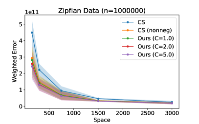
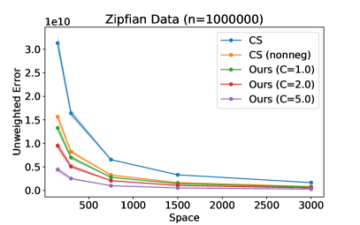
Figure 6: Comparison of weighted and unweighted error without predictions on Zipfian data.

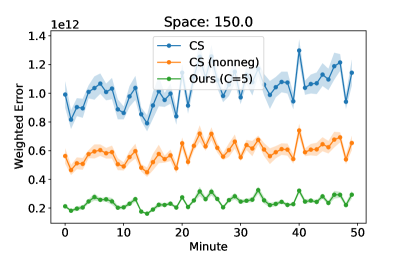
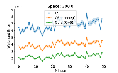
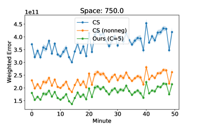
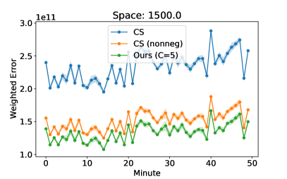
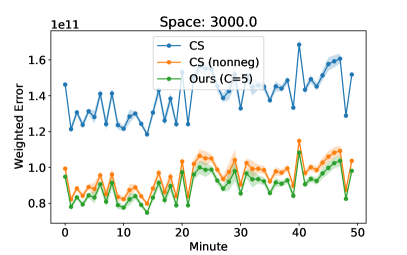
Figure 7: Comparison of weighted errors without predictions on the CAIDA dataset

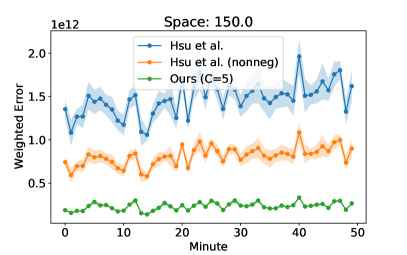
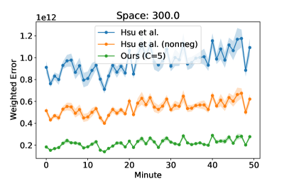
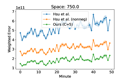
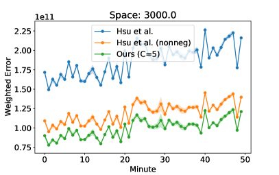
Figure 8: Comparison of weighted errors with predictions on the CAIDA dataset

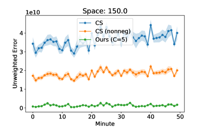
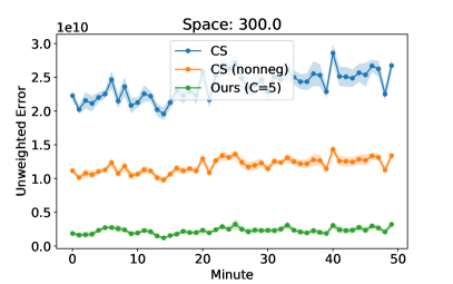
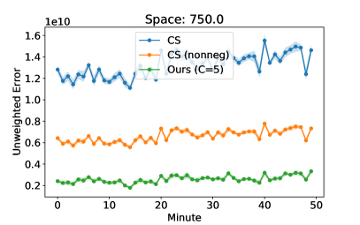
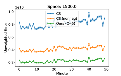
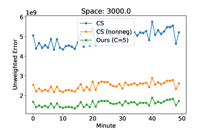
Figure 9: Comparison of unweighted errors without predictions on the CAIDA dataset

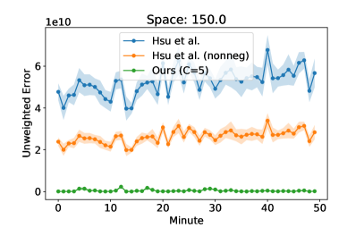
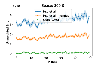
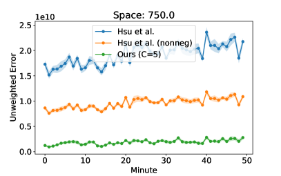
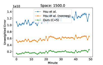
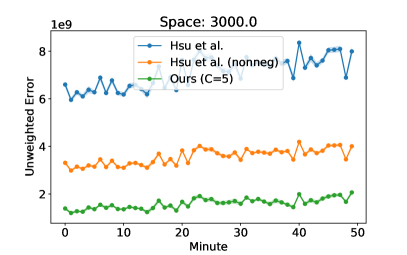
Figure 10: Comparison of unweighted errors with predictions on the CAIDA dataset

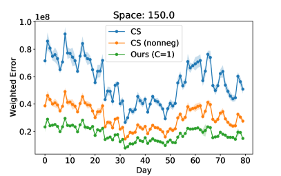
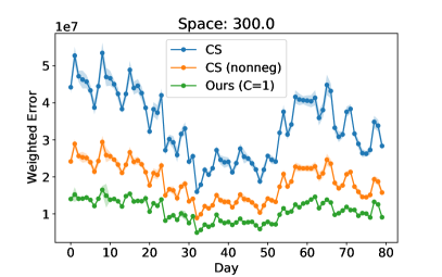
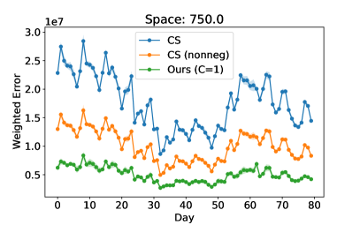
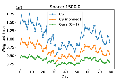
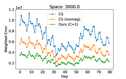
Figure 11: Comparison of weighted errors without predictions on the AOL dataset

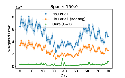
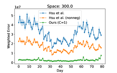
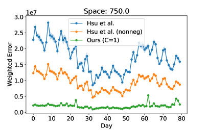
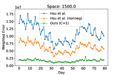
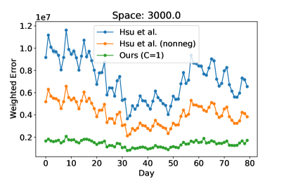
Figure 12: Comparison of weighted errors with predictions on the AOL dataset

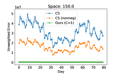
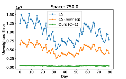
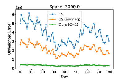
Figure 13: Comparison of unweighted errors without predictions on the AOL dataset

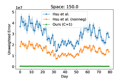
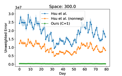
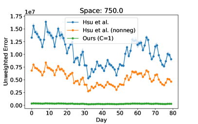
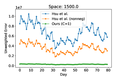
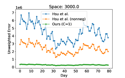
Figure 14: Comparison of unweighted errors with predictions on the AOL dataset

References

• [1] Anders Aamand, Justin Y. Chen, and Piotr Indyk. (Optimal) Online Bipartite Matching with Degree Information. In Advances in Neural Information Processing Systems, volume 35, 2022.
• [2] Noga Alon, Yossi Matias, and Mario Szegedy. The space complexity of approximating the frequency moments. In Proceedings of the twenty-eighth annual ACM symposium on Theory of computing, pages 20–29, 1996.
• [3] Amirali Aghazadeh and Ryan Spring and Daniel LeJeune and Gautam Dasarathy and Anshumali Shrivastava and Richard G. Baraniuk. Mission: Ultra large-scale feature selection using count-sketches. In International Conference on Machine Learning, pages 80–88. PMLR, 2018.
• [4] Keerti Anand, Rong Ge, and Debmalya Panigrahi. Customizing ml predictions for online algorithms. In International Conference on Machine Learning, pages 303–313, 2020.
• [5] Spyros Angelopoulos, Christoph Dürr, Shendan Jin, Shahin Kamali, and Marc Renault. Online computation with untrusted advice. In 11th Innovations in Theoretical Computer Science Conference (ITCS 2020). Schloss Dagstuhl-Leibniz-Zentrum für Informatik, 2020.
• [6] Antonios Antoniadis, Christian Coester, Marek Eliáš, Adam Polak, and Bertrand Simon. Online metric algorithms with untrusted predictions. ACM Transactions on Algorithms, 19(2):1–34, 2023.
• [7] Maria-Florina Balcan, Travis Dick, Tuomas Sandholm, and Ellen Vitercik. Learning to branch. In International Conference on Machine Learning, pages 353–362, 2018.
• [8] George Bennett. Probability inequalities for the sum of independent random variables. Journal of the American Statistical Association, 57(297):33–45, 1962.
• [9] Aditya Bhaskara, Ashok Cutkosky, Ravi Kumar, and Manish Purohit. Logarithmic regret from sublinear hints. In Advances in Neural Information Processing Systems 34: Annual Conference on Neural Information Processing Systems 2021, pages 28222–28232, 2021.
• [10] Oscar Boykin, Avi Bryant, Edwin Chen, ellchow, Mike Gagnon, Moses Nakamura, Steven Noble, Sam Ritchie, Ashutosh Singhal, and Argyris Zymnis. Algebird. https://twitter.github.io/algebird/, 2016.
• [11] Vladimir Braverman, Stephen R Chestnut, Nikita Ivkin, Jelani Nelson, Zhengyu Wang, and David P Woodruff. Bptree: an l2 heavy hitters algorithm using constant memory. In Proceedings of the 36th ACM SIGMOD-SIGACT-SIGAI Symposium on Principles of Database Systems, pages 361–376, 2017.
• [12] CAIDA. Caida internet traces, chicago. http://www.caida.org/data/monitors/passive-equinix-chicago.xml, 2016.
• [13] Emmanuel J Candès, Justin Romberg, and Terence Tao. Robust uncertainty principles: Exact signal reconstruction from highly incomplete frequency information. IEEE Transactions on information theory, 52(2):489–509, 2006.
• [14] Moses Charikar, Kevin Chen, and Martin Farach-Colton. Finding frequent items in data streams. In International Colloquium on Automata, Languages, and Programming, pages 693–703. Springer, 2002.
• [15] Justin Y. Chen, Talya Eden, Piotr Indyk, Honghao Lin, Shyam Narayanan, Ronitt Rubinfeld, Sandeep Silwal, Tal Wagner, David P. Woodruff, and Michael Zhang. Triangle and four cycle counting with predictions in graph streams. In 10th International Conference on Learning Representations, ICLR, 2022.
• [16] Justin Y. Chen, Sandeep Silwal, Ali Vakilian, and Fred Zhang. Faster fundamental graph algorithms via learned predictions. In International Conference on Machine Learning, ICML, volume 162 of Proceedings of Machine Learning Research, pages 3583–3602, 2022.
• [17] Herman Chernoff. A measure of asymptotic efficiency for tests of a hypothesis based on the sum of observations. Annals of Mathematical Statistics, 23(4):493–507, 1952.
• [18] Kenneth L Clarkson and David P Woodruff. Low-rank approximation and regression in input sparsity time. Journal of the ACM (JACM), 63(6):1–45, 2017.
• [19] Edith Cohen, Ofir Geri, and Rasmus Pagh. Composable sketches for functions of frequencies: Beyond the worst case. In Proceedings of the 37th International Conference on Machine Learning, 2020.
• [20] Graham Cormode and Shan Muthukrishnan. An improved data stream summary: the count-min sketch and its applications. Journal of Algorithms, 55(1):58–75, 2005.
• [21] Erik D Demaine, Alejandro López-Ortiz, and J Ian Munro. Frequency estimation of internet packet streams with limited space. In Esa, volume 2, pages 348–360. Citeseer, 2002.
• [22] Ilias Diakonikolas, Vasilis Kontonis, Christos Tzamos, Ali Vakilian, and Nikos Zarifis. Learning online algorithms with distributional advice. In International Conference on Machine Learning, pages 2687–2696, 2021.
• [23] Michael Dinitz, Sungjin Im, Thomas Lavastida, Benjamin Moseley, and Sergei Vassilvitskii. Faster matchings via learned duals. Advances in neural information processing systems, 34:10393–10406, 2021.
• [24] Yihe Dong, Piotr Indyk, Ilya Razenshteyn, and Tal Wagner. Learning sublinear-time indexing for nearest neighbor search. arXiv preprint arXiv:1901.08544, 2019.
• [25] David L Donoho. Compressed sensing. IEEE Transactions on information theory, 52(4):1289–1306, 2006.
• [26] Marina Drygala, Sai Ganesh Nagarajan, and Ola Svensson. Online algorithms with costly predictions. In Proceedings of The 26th International Conference on Artificial Intelligence and Statistics, volume 206 of Proceedings of Machine Learning Research, pages 8078–8101. PMLR, 2023.
• [27] Elbert Du, Franklyn Wang, and Michael Mitzenmacher. Putting the “learning" into learning-augmented algorithms for frequency estimation. In Proceedings of the 38th International Conference on Machine Learning, pages 2860–2869, 2021.
• [28] Talya Eden, Piotr Indyk, Shyam Narayanan, Ronitt Rubinfeld, Sandeep Silwal, and Tal Wagner. Learning-based support estimation in sublinear time. In 9th International Conference on Learning Representations, ICLR, 2021.
• [29] Paul Erdős. On a lemma of littlewood and offord. Bulletin of the American Mathematical Society, 51(12):898–902, 1945.
• [30] Jon C. Ergun, Zhili Feng, Sandeep Silwal, David P. Woodruff, and Samson Zhou. Learning-augmented $k$-means clustering. In 10th International Conference on Learning Representations, ICLR, 2022.
• [31] Cristian Estan and George Varghese. New directions in traffic measurement and accounting: Focusing on the elephants, ignoring the mice. ACM Transactions on Computer Systems (TOCS), 21(3):270–313, 2003.
• [32] Sreenivas Gollapudi and Debmalya Panigrahi. Online algorithms for rent-or-buy with expert advice. In Proceedings of the 36th International Conference on Machine Learning, pages 2319–2327, 2019.
• [33] Amit Goyal, Hal Daumé III, and Graham Cormode. Sketch algorithms for estimating point queries in nlp. In Proceedings of the 2012 joint conference on empirical methods in natural language processing and computational natural language learning, pages 1093–1103, 2012.
• [34] Anupam Gupta, Debmalya Panigrahi, Bernardo Subercaseaux, and Kevin Sun. Augmenting online algorithms with $\varepsilon$-accurate predictions. Advances in Neural Information Processing Systems, 35:2115–2127, 2022.
• [35] Wassily Hoeffding. Probability inequalities for sums of bounded random variables. Journal of the American Statistical Association, 58(301):13–30, 1963.
• [36] Chen-Yu Hsu, Piotr Indyk, Dina Katabi, and Ali Vakilian. Learning-based frequency estimation algorithms. In 7th International Conference on Learning Representations, ICLR 2019, New Orleans, LA, USA, May 6-9, 2019. OpenReview.net, 2019.
• [37] Sungjin Im, Ravi Kumar, Aditya Petety, and Manish Purohit. Parsimonious learning-augmented caching. In International Conference on Machine Learning, pages 9588–9601. PMLR, 2022.
• [38] Piotr Indyk, Ali Vakilian, and Yang Yuan. Learning-based low-rank approximations. In Advances in Neural Information Processing Systems, pages 7400–7410, 2019.
• [39] Tanqiu Jiang, Yi Li, Honghao Lin, Yisong Ruan, and David P. Woodruff. Learning-augmented data stream algorithms. In International Conference on Learning Representations, 2020.
• [40] Richard M Karp, Scott Shenker, and Christos H Papadimitriou. A simple algorithm for finding frequent elements in streams and bags. ACM Transactions on Database Systems (TODS), 28(1):51–55, 2003.
• [41] Elias Khalil, Hanjun Dai, Yuyu Zhang, Bistra Dilkina, and Le Song. Learning combinatorial optimization algorithms over graphs. In Advances in Neural Information Processing Systems, pages 6348–6358, 2017.
• [42] Tim Kraska, Alex Beutel, Ed H Chi, Jeffrey Dean, and Neoklis Polyzotis. The case for learned index structures. In Proceedings of the 2018 International Conference on Management of Data, pages 489–504, 2018.
• [43] Silvio Lattanzi, Thomas Lavastida, Benjamin Moseley, and Sergei Vassilvitskii. Online scheduling via learned weights. In Proceedings of the Fourteenth Annual ACM-SIAM Symposium on Discrete Algorithms, pages 1859–1877. SIAM, 2020.
• [44] Yi Li, Honghao Lin, Simin Liu, Ali Vakilian, and David Woodruff. Learning the positions in countsketch. In 11th International Conference on Learning Representations, ICLR, 2023.
• [45] John Edensor Littlewood and Albert C Offord. On the number of real roots of a random algebraic equation. ii. In Mathematical Proceedings of the Cambridge Philosophical Society, volume 35, pages 133–148. Cambridge University Press, 1939.
• [46] Zaoxing Liu, Antonis Manousis, Gregory Vorsanger, Vyas Sekar, and Vladimir Braverman. One sketch to rule them all: Rethinking network flow monitoring with univmon. In Proceedings of the 2016 ACM SIGCOMM Conference, pages 101–114, 2016.
• [47] Thodoris Lykouris and Sergei Vassilvitskii. Competitive caching with machine learned advice. In International Conference on Machine Learning, pages 3302–3311, 2018.
• [48] Gurmeet Singh Manku and Rajeev Motwani. Approximate frequency counts over data streams. In VLDB’02: Proceedings of the 28th International Conference on Very Large Databases, pages 346–357. Elsevier, 2002.
• [49] Ahmed Metwally, Divyakant Agrawal, and Amr El Abbadi. Efficient computation of frequent and top-k elements in data streams. In International Conference on Database Theory, pages 398–412. Springer, 2005.
• [50] Gregory T Minton and Eric Price. Improved concentration bounds for count-sketch. In Proceedings of the twenty-fifth annual ACM-SIAM symposium on Discrete algorithms, pages 669–686. Society for Industrial and Applied Mathematics, 2014.
• [51] Jayadev Misra and David Gries. Finding repeated elements. Science of computer programming, 2(2):143–152, 1982.
• [52] Michael Mitzenmacher. A model for learned bloom filters and optimizing by sandwiching. In Advances in Neural Information Processing Systems, pages 464–473, 2018.
• [53] Michael Mitzenmacher. Scheduling with predictions and the price of misprediction. In 11th Innovations in Theoretical Computer Science Conference (ITCS 2020). Schloss Dagstuhl-Leibniz-Zentrum für Informatik, 2020.
• [54] Thy Nguyen, Anamay Chaturvedi, and Huy Le Nguyen. Improved learning-augmented algorithms for $k$-means and $k$-medians clustering. 2023.
• [55] Greg Pass, Abdur Chowdhury, and Cayley Torgeson. A picture of search. In Proceedings of the 1st international conference on Scalable information systems, pages 1–es, 2006.
• [56] Manish Purohit, Zoya Svitkina, and Ravi Kumar. Improving online algorithms via ml predictions. In Advances in Neural Information Processing Systems, pages 9661–9670, 2018.
• [57] Sandeep Silwal, Sara Ahmadian, Andrew Nystrom, Andrew McCallum, Deepak Ramachandran, and Seyed Mehran Kazemi. Kwikbucks: Correlation clustering with cheap-weak and expensive-strong signals. In The Eleventh International Conference on Learning Representations, 2023.
• [58] Partha Talukdar and William Cohen. Scaling graph-based semi supervised learning to large number of labels using count-min sketch. In Artificial Intelligence and Statistics, pages 940–947. PMLR, 2014.
• [59] Jun Wang, Wei Liu, Sanjiv Kumar, and Shih-Fu Chang. Learning to hash for indexing big data - a survey. Proceedings of the IEEE, 104(1):34–57, 2016.
• [60] Alexander Wei and Fred Zhang. Optimal robustness-consistency trade-offs for learning-augmented online algorithms. Advances in Neural Information Processing Systems, 33:8042–8053, 2020.
• [61] David P Woodruff et al. Sketching as a tool for numerical linear algebra. Foundations and Trends® in Theoretical Computer Science, 10(1–2):1–157, 2014.
• [62] Minlan Yu, Lavanya Jose, and Rui Miao. Software defined traffic measurement with opensketch. In NSDI, volume 13, pages 29–42, 2013.
• [63] Matei Zaharia, Reynold S Xin, Patrick Wendell, Tathagata Das, Michael Armbrust, Ankur Dave, Xiangrui Meng, Josh Rosen, Shivaram Venkataraman, Michael J Franklin, et al. Apache spark: a unified engine for big data processing. Communications of the ACM, 59(11):56–65, 2016.