Continuum extrapolated high order baryon fluctuations

Abstract

Fluctuations play a key role in the study of QCD phases. Lattice QCD is a valuable tool to calculate them, but going to high orders is challenging. Up to the fourth order, continuum results are available since 2015. We present the first continuum results for sixth order baryon fluctuations for temperatures between $T=130-200\,{\rm MeV}$, and eighth order at $T=145\,{\rm MeV}$ in a fixed volume. We show that for $T\leq 145\,{\rm MeV}$, relevant for criticality search, finite volume effects are under control. Our results are in sharp contrast with well known results in the literature obtained at finite lattice spacing.

1. Introduction: fluctuations and QCD phases: The main goal of the heavy ion program of many accelerator facilities (e.g., at LHC, RHIC or the upcoming CBM/FAIR) is to create new phases of matter and explore their properties under extreme conditions. Several experimental programs (such as the Beam Energy Scan program at RHIC [1, 2]) are designed to search for a hypothetical critical end point in the temperature-baryon density phase diagram. Some of the most important observables in this quest are fluctuations of conserved charges. In the grand canonical ensemble, they are derivatives of the pressure with respect to the chemical potentials coupled to the charges. In this work, we will calculate such fluctuation observables at zero baryochemical potential.

The physics applications of fluctuation observables are numerous. First, the equation of state of the hot-and-dense quark gluon plasma is one of the main inputs of lattice QCD to the phenomenology of heavy ion physics. Fluctuations at zero baryochemical potential $\mu_{B}$ are the basis for extrapolations of the QCD equation of state to non-zero $\mu_{B}$, both by means of a truncated Taylor expansion [3], as well as via different resummations of the Taylor series [4, 5, 6].

Second, fluctuation observables are sensitive to criticality. While first-principle lattice simulations have shown that the chiral transition is a crossover at zero baryon density [7], at larger baryon densities several model calculations predict a critical endpoint in the 3D Ising universality class [8, 9, 10, 11], where the crossover line becomes a line of first order transitions. One of the proposed experimental signatures of such a critical endpoint is a non-monotonic behavior of the fourth-to- second order baryon number fluctuations as a function of $\mu_{B}$ [12, 13]. The extrapolation of this ratio to $\mu_{B}>0$ is possible, if a sufficient number of Taylor coefficients (fluctuations) are available at $\mu_{B}=0$. Thus, fluctuations at $\mu_{B}=0$ are also important for the quest to find the critical endpoint. An important baseline in this search is given by the hadron resonance gas (HRG) model, a non-critical model that describes thermodynamics below the chiral transition at $\mu_{B}=0$ remarkably well. A reasonable minimum criterium for criticality searches, then, is the presence of solid deviations between HRG predictions and equilibrium QCD.

A different type of criticality - in the O(4) universality class - is also expected to be present in QCD, related to chiral symmetry restoration, one of the most important concepts in heavy ion physics. In the limit of zero light quark masses, the $SU(2)\times SU(2)$ chiral symmetry becomes exact, and the crossover transition occurring at physical masses is expected to be replaced by a genuine second order transition  [14, 15, 16]. Through the presence of a single scaling variable (a combination of the quark masses, the temperature and the chemical potential), O(4) criticality has imprints on the temperature dependence of higher baryon number fluctuations at $\mu_{B}=0$ up to physical values of the quark masses (for a model calculation, see e.g. Ref. [17]). The presence of such an O(4) scaling regime is likely the reason why lattice QCD calculation see no sharpening or strengthening of the crossover transition for small chemical potentials [18, 19, 4]. The complicated interplay of O(4) and Ising criticality motivates more involved theoretical approaches to the phase diagram, based on Lee-Yang zeroes [20, 21], which have gained popularity in recent years [22, 23, 24, 25, 26]. These approaches, too, require reliable determinations of the corresponding fluctuations.

Third, fluctuation observables are very sensitive to the degrees of freedom of a thermodynamic system. This fact has been used before to argue, e.g., the existence of further (yet undiscovered) resonances [27, 28, 29] in the hadron spectrum, which was later confirmed by experiment [30].

Finally, fluctuation observables are central in the study of chemical freezeout in heavy ion collisions. This is an especially interesting avenue of research, since it has the potential of allowing a direct comparison between first-principle QCD predictions and experimental data. While the comparison itself has many caveats, due to experimental effects [31, 32, 33], it is obviously worth pursuing.

2. Current lattice estimates: Conserved charge fluctuations have been a focus of lattice simulations for well over a decade now. Like any other observable, a reliable calculation of these requires a continuum limit extrapolation, via simulations using smaller-and-smaller lattice spacings. Up to second order, they are known in the continuum since 2012 [34]. Fourth order fluctuations in the baryon number and strangeness were first continuum extrapolated in 2015 [35]. In that case, a large temperature range was considered, showing good agreement with the hadron resonance gas model at low temperatures, as well as good agreement with perturbative calculations [36, 37] at high temperatures. Since then, calculations of the fourth order coefficients were pushed to very high precision [38]. Thus, up to fourth order, the derivatives in full QCD are known accurately, with the exception of electric charge fluctuations, which suffer from large cut-off effects that make continuum extrapolations difficult [35].

At the sixth and eighth orders, the statistics requirements for the direct determination of the coefficients dramatically blow up, thus, a continuum extrapolation of these coefficients has never been attempted. Because of the high statistics required, all available results on higher fluctuations employ the computationally cheapest discretization: staggered fermions. These suffer from a lattice artefact called taste breaking [39, 40], whose effect is to strongly distort the meson spectrum at a finite spacing. One might think that, since baryon number fluctuations directly couple to baryons only, and not mesons, this issue is of no great importance here. Unfortunately, this is only the case at the level of the baryon number $B=1$ sector of the Hilbert space. Two-baryon interactions are mediated by mesons, and thus, taste breaking distorting meson physics can have relevant effects on the description of baryon dense matter (or, equivalently, on high order fluctuations at $\mu_{B}=0$). In fact, the higher the order of the fluctuations, the larger the effect of multi-baryon interactions on them. Hence, these fluctuations could be particularly sensitive to taste breaking effects. On a more basic level, higher order $\mu_{B}$-derivatives probe physics at larger $\mu_{B}$, which at a finite spacing will be closer to the cut-off scale of $1/a$ ($a$ being the lattice spacing), making cut-off effects potentially important.

The statistics required for the calculation of higher order fluctuations can be drastically reduced by introducing a purely imginary chemical potential, calculating lower order fluctuations, and fitting their functional dependence on the imaginary chemical potential. The price for this reduction in statistics requirements is that assumptions have to be made on the functional form of the lower order fluctuations, leading to hard-to-control systematic errors.

So far, three collaborations have presented results up to the eighth order with improved lattice actions. In chronological order: First, the Pisa group presented results on lattices with 6 timeslices of 2stout improved fermions [7, 41] in Ref. [42]. Second, the Wuppertal-Budapest collaboration presented results with 12 timeslices of 4stout improved fermions [43] in Ref. [44]. These two calculations took advantage of simulations at imaginary chemical potential. Finally, the HotQCD collaboration presented results with 8 timeslices of HISQ fermions [45], using a direct determination at $\mu_{B}=0$ (i.e., without imaginary $\mu_{B}$ simulations) in Refs. [38, 6]. For the latter calculation, two orders of magnitude more statistics were collected, compared to the previous two. It is a testament to the efficacy of the imaginary chemical potential method, then, that the error bars on the imaginary chemical potential calculations of the sixth and eighth order coefficients are substantially smaller.

At the current level of precision, discrepancies emerge between the calculations. In particular, the results based on the imaginary chemical potential method are in good agreement with the hadron resonance gas model for low temperatures. On the other hand, the direct calculation shows significant deviations for both observables even at the lowest temperature considered. To shed light on QCD criticality, this discrepancy has to be resolved.

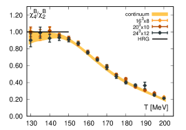
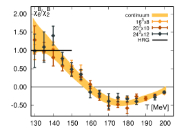
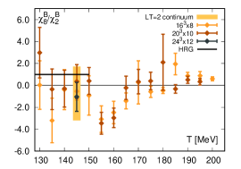
Figure 1: Our lattice results for the ratios $\chi^{B}_{4}/\chi^{B}_{2}$ (left), $\chi^{B}_{6}/\chi^{B}_{2}$ (center), $\chi^{B}_{8}/\chi^{B}_{2}$ (right). For the first two, the continuum extrapolation is shown as a yellow band. HRG model predictions are shown as solid black lines in all cases.

In addition to the different extraction method for the higher order coefficients (direct at $\mu_{B}=0$ vs indirect from $\mu_{B}^{2}\leq 0$), a potentially more significant difference between the two types of calculation lies in how the chemical potential is defined. Due to the extreme cost of the direct method, for fluctuations of order six and higher, the chemical potential in that case was introduced via the so-called linear prescription. In the other two cases, the exponential definition was used. Derivatives with respect to the chemical potential can be shown to be UV finite by virtue of a $U(1)$ symmetry if the chemical potential is introduced like a constant imaginary gauge field [46]. This is the exponential definition. If, instead, a naive linear definition is employed, power-law UV divergences appear in the free energy already in the case of free quarks. By taking enough derivatives with respect to the chemical potential, such power-law divergences disappear. However, this is not the case for logarithmic divergences, the absence of which for the naive linear definition is not proven for the interacting theory. Thus, although the linear definition is computationally cheaper, care should be taken in considering these results.

The linear definition also breaks the exact Roberge-Weiss periodicity [47] of the partition function. Even if one assumes that there are no problems with logarithmic divergences, the loss of Roberge-Weiss periodicity with the linear definition can potentially lead to large cut-off effects, since it effectively means that at a finite spacing, in contrast to the continuum, the free energy gets contributions from Hilbert subpsaces not only at integer, but also at non-integer values of the baryon number, which at the very least, is a non-physical feature at finite spacing.

3. Lattice calculation of fluctuations up to eighth order

In this letter, we present the first continuum results for baryon fluctuations up to the sixth order for temperatures between $T=130-200\,{\rm MeV}$, and up to the eighth order for a temperature of $T=145\,{\rm MeV}$. Continuum extrapolation is made possible by the introduction of a new discretization, which we call the 4HEX action, that strongly suppresses taste breaking effects compared to all available actions in the literature. Although more costly, we pursue a direct determination at $\mu_{B}=0$, in order to avoid possible systematic effects due to a choice of fit ansatz, necessary for the imaginary chemical potential method. Moreover, in order to avoid possible issues with the introduction of the chemical potential, we employ the exponential definition to all orders. Due to the extreme statistics cost of the direct method, this endeavour is only feasible in a volume that is smaller than what is typically used in the field, with an aspect ratio $LT=2$. Thanks to the availability in the literature of the aforementioned results at finite lattice spacing, but with larger volume, we are able to show that below $T=145\,{\rm MeV}$, finite volume effects in our results are under control. Note that this is the relevant temperature range for the search for the elusive critical endpoint of QCD.

The novel lattice action we use for this thermodynamics study, 4HEX, is based on rooted staggered fermions with 4 steps of HEX smearing [48] with physical quark masses, and the DBW2 gauge action [49]. This lattice action benefits from dramatically reduced taste breaking effects, compared to all other actions used in the literature. We simulate $16^{3}\times 8$, $20^{2}\times 10$ and $24^{3}\times 12$ lattices to obtain a well-controlled continuum extrapolation. Details on the 4HEX action, the scale setting procedure, and the systematic error estimation can be found in the supplemental material.

We calculate fluctuations of the baryon number at zero strangeness chemical potential:

$$\chi^{B}_{n}\equiv\left(\frac{\partial^{n}(p/T^{4})}{\partial(\mu_{B}/T)^{n}}\right)_{\mu_{S}=0}\rm.$$ (1)

We also include results on the strangeness neutral line $n_{s}\equiv 0$ in the Supplemental Material, which lead to similar conclusions as in the $\mu_{S}=0$ case.

We use the exponential definition of the chemical potential at all orders in $\mu_{B}$ on all our lattices. For the $N_{\tau}=8,10$ lattices, we use the reduced matrix formalism to calculate the fluctuations, in the same way as we did in Refs. [50, 51]. For the $N_{\tau}=12$ lattice, we use the standard random source method [52].

We show our continuum extrapolated results for $\chi^{B}_{4}/\chi^{B}_{2}$ (left) and $\chi^{B}_{6}/\chi^{B}_{2}$ (center), together with the corresponding finite lattice spacing results in Fig. 1. The continuum results are obtained together with a spline fit of the temperature dependence. The exact procedure is described in the Supplemental Material. The bands include statistical and systematic uncertainties, consisting of different scale settings and different spline fits of the data. The covered temperature range is $130\,{\rm MeV}\leq T\leq 200\,{\rm MeV}$. Also shown are the results on the $N_{\tau}=8,10$ lattices for $\chi^{B}_{8}/\chi^{B}_{2}$ (right). For this observable, we also include the continuum extrapolation at a single temperature of $T=145\,{\rm MeV}$. Hadron resonance gas predictions are shown, and they equal 1 in all cases independently from the temperature and the hadron spectrum used.

From Fig. 1, it is apparent how small the cut-off effects of the 4HEX action are, as is the fact that, for $T<145\,{\rm MeV}$, the fluctuations in continuum QCD are in very good agreement with the HRG results.

4. Comparisons with the literature:

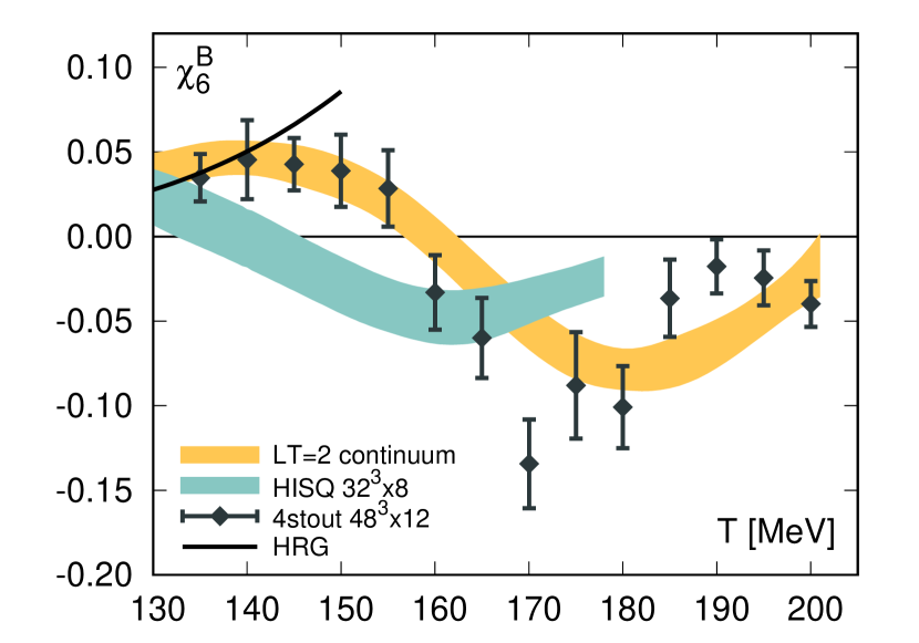
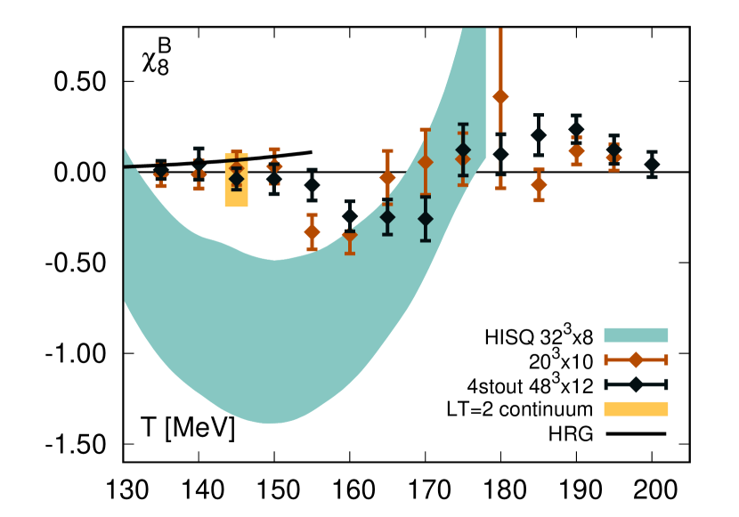
Figure 2: Our results for sixth (top) and eighth (bottom) order baryon number susceptibilities. The HISQ (splined) results are shown as light blue bands, and the 4stout results are shown are black points. Our new results are shown as a yellow band for the continuum extrapolation of $\chi_{6}^{B}$ and the continuum extrapolation of $\chi_{8}^{B}$ (at $T=145\,{\rm MeV}$), and as brown points for $\chi_{8}^{B}$ on the $20^{3}\times 10$ lattice. HRG model predictions are shown as solid black lines.

Being our results on the sixth and eighth order fluctuations the first ever continuum extrapolated, we proceed to compare them to previous results from the literature, with an aspect ratio $LT=4$. In the top panel of Fig. 2, we show the continuum $\chi^{B}_{6}$ (yellow band) alongside previous results by the Wuppertal-Budapest collaboration obtained with the imaginary chemical potential method using 12 timeslices of 4stout improved staggered fermions [44] (black points), and results by the HotQCD collaboration obtained with the direct method and 8 time slices of HISQ fermions [6] (green band). The latter are not direct data, but rather come from a spline interpolation of the direct data. The comparison is fair, since we also use a spline interpolation on our data, to allow for systematic error estimation on the continuum limit. The role of the spline interpolation in thermodynamics studies is to i) reduce the random noise on the direct data, by utilizing continuity in $T$ and to ii) allow one to take temperature derivatives, which are needed for the calculation of certain thermodynamic quantities, such as the speed of sound. The HotQCD collaboration has also used the splined version of their results on high order fluctuations in determining phenomenological quantities (see, e.g., Ref. [6]). Looking at the three results in comparison, a very simple interpretation emerges. First, at temperatures below $145\,{\rm MeV}$, our results at $N_{\tau}=12$ agree with our new continuum extrapolated results, even though the volume is different in the two simulations. On the other hand, the $N_{\tau}=8$ HotQCD result does not agree with our old $N_{\tau}=12$ results, even though the physical volumes are the same. This means that, at low temperatures, finite volume effects are small and cut-off effects are large. It appears that these $N_{\tau}=8$ lattices are too coarse for phenomenological applications. The $N_{\tau}=8$ results show very significant deviations from the hadron resonance gas. For example, it is noteworthy that the sign of $d\chi^{B}_{6}/dT$ is opposite to the HRG model prediction at all these low temperatures. Such deviations turned out to be cut-off effects, since the continuum extrapolated results show good quantitative agreement with the HRG.

A similar scenario appears in the bottom panel of Fig. 2, where we compare our new results on $20^{3}\times 10$ lattices with results from the same $LT=4$ simulations – Wuppertal-Budapest $N_{\tau}=12$ [44] (black points) and HotQCD $N_{\tau}=8$ [6] (green band) – as shown in the case of $\chi_{6}^{B}$. We also include our new continuum extrapolation at $T=145\,{\rm MeV}$. Besides the markedly smaller errors, our results are in good agreement with each other, showing small volume dependence especially at lower temperature. Moreover, quantitative agreement with HRG model predictions is evident up to $T=145\,{\rm MeV}$. Our continuum result at $T=145\,{\rm MeV}$ confirms these findings. As in the previous case, it appears that cut-off effects for $T\leq 145\,{\rm MeV}$ are too large to allow for a safe use of results on coarse lattices for phenomenological applications. Finally, we note that the for $T>145\,{\rm MeV}$, our old $N_{\tau}=12$ large volume and new $N_{\tau}=10$ small volume results do not agree. In particular, the local minimum of $\chi^{B}_{8}$ is shifted to lower temperatures. This is likely a finite volume effect, due to the crossover transition moving to slightly lower $T$ in a smaller volume.

5. Discussion: In this letter we have reported the first continuum extrapolated results for high order baryon number fluctuations available in the literature. By means of a novel discretization of the QCD action, we were able to carry out a continuum extrapolation using lattice with 8,10 and 12 time slices. We used an aspect ratio of $LT=2$. We calculated sixth order fluctuations in the continuum in a temperature range between $T=130-200\,{\rm MeV}$. We also calculated the eighth order fluctuations in the continuum at a single temperature $T=145\,{\rm MeV}$. A comparison of our results with existing results at finite lattice spacing and larger physical volumes showed that, in the temperature regime relevant for the critical point search, volume effects are well under control already for the smaller volume used in our study. In contrast, cut-off effects in previous results in the literature where not always under control, especially at the lower temperatures relevant for constraining the position of the critical endpoint. Thus, phenomenological conclusions based on erroneous coefficients ought to be reexamined in the near future. These include estimates of the radius of convergence and poles of Padé approximants, used to constrain the location of the critical endpoint and the convergence of the Taylor expansion for the equation of state, used as input for hydrodynamic simulations as well as estimates of fluctuation observables at $\mu_{B}>0$ used to study chemical freeze-out. We plan to revisit all of these points in future publications.

Acknowledgements: The project was supported by the BMBF Grant No. 05P21PXFCA. This work is also supported by the MKW NRW under the funding code NW21-024-A. Further funding was received from the DFG under the Project No. 496127839. This work was also supported by the Hungarian National Research, Development and Innovation Office, NKFIH Grant No. KKP126769. This work was also supported by the NKFIH excellence grant TKP2021_NKTA_64. D.P. is supported by the ÚNKP-23-3 New National Excellence Program of the Ministry for Culture and Innovation from the source of the National Research, Development and Innovation Fund. The authors gratefully acknowledge the Gauss Centre for Supercomputing e.V. (www.gauss-centre.eu) for funding this project by providing computing time on the GCS Supercomputers Juwels-Booster at Juelich Supercomputer Centre and HAWK at Höchstleistungsrechenzentrum Stuttgart.

I Supplemental material

4HEX action

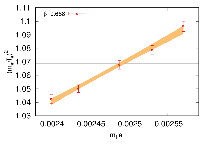
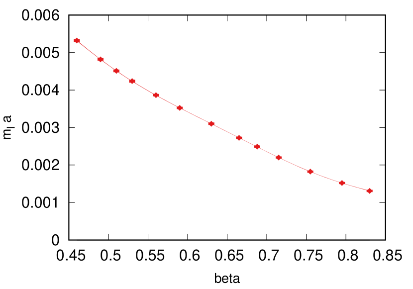
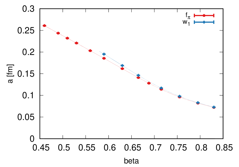
Figure 3: Top: Example of quark mass tuning for simulations at $\beta=0.688$. The orange band is a linear fit of the data, and the black line is the target value of the ratio $m_{\pi}^{2}/f_{\pi}^{2}$. Center: Line of constant physics i.e., light quark mass as a function of the inverse bare gauge coupling. The points show the direct determination from the procedure in the top panel, the band is a polynomial fit as a function of $\beta$. Bottom: lattice spacing as determined through the pion decay constant (red) and $w_{1}$ scale (orange). The band is a polynomial fit as a function of the coupling $\beta$.

In this work we employ simulations with $N_{f}=2+1+1$ staggered dynamical quark flavours with physical masses. In the gauge sector we use the DBW2 action [49], and in the fermion sector we use links with 4 levels of HEX smearing [48].

Before quantitative results can be extracted, the action must be parameterized, meaning that the dependence of the bare quark masses on the gauge coupling must be tuned, so that the theory is renormalized in the parameter range of interest. In our simulations we used degenerate up and down quark masses, and fixed the light- strange mass ratio to $m_{s}/m_{ud}=27.63$, and the strange-charm mass ratio to $m_{c}/m_{s}=11.85$. In order to tune the light quark mass, we used the ratio $m_{\pi}/f_{\pi}=1.0337$, where we used the isospin-averaged pion mass $m_{\pi}=134.8\,{\rm MeV}$ [53] and the pion decay constant $f_{\pi}=130.41\,{\rm MeV}$. In order to adopt a proper comparison, we corrected both $m_{\pi}$ and $f_{\pi}$ for finite volume effects using results from two-flavour chiral perturbation theory [54]. For each value of the coupling, we simulated 3-5 values of the quark masses, then extracted the tuned masses via a linear interpolation in $m_{\pi}^{2}/f_{\pi}^{2}$. An example of the mass tuning for $\beta=0.688$ is shown in the top panel of Fig. 3.

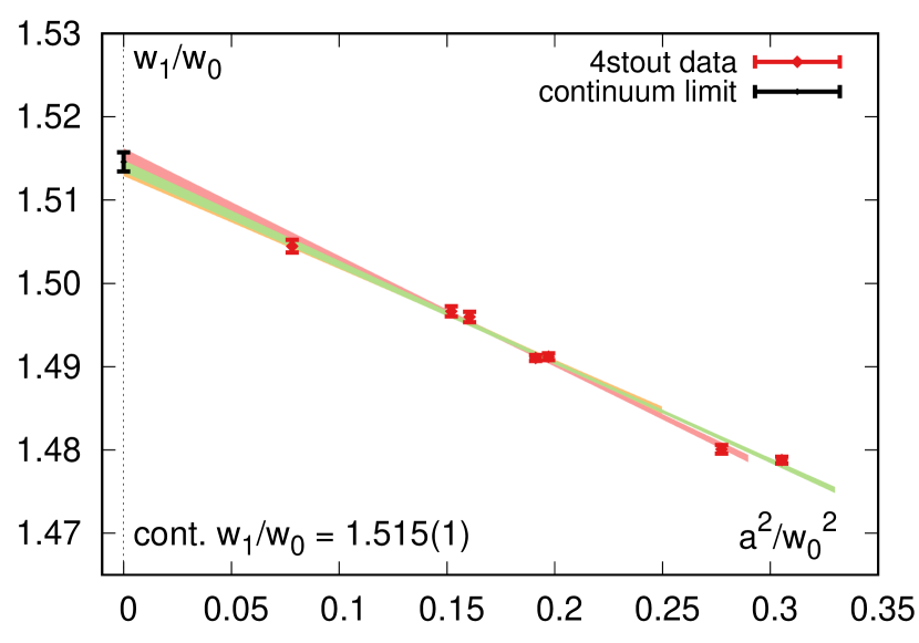
Figure 4: Continuum limit of the ratio $w_{1}/w_{0}$ from 4stout simulations.

We parameterized the action in the range $\beta=0.46-0.83$, corresponding to lattice spacings in the range $a=0.261-0.072\,{\rm fm}$. The line of constant physics is shown over the whole range in the center panel of Fig. 3. We set the scale with the pion decay constant $f_{\pi}$, as well as with a modified version of the Wilson-flow-based $w_{0}$ [55], which we refer to as $w_{1}$. Both scale settings are shown in the bottom panel of Fig. 3. The definition for $w_{0}$ is the following:

$$\left.W(t)\right|_{t=w^{2}_{0}}=0.3\,\,,$$ (2)

where $t$ is the flow time, and $W(t)$ is defined as:

$$W(t)\equiv t\frac{d}{dt}\left\{t^{2}\left\langle E(t)\right\rangle\right\}\,\,,$$ (3)

where, in turn, $\left\langle E(t)\right\rangle$ is the expectation value of the continuum-like action density $G^{a}_{\mu\nu}(t)G^{a}_{\mu\nu}(t)/4$. The quantity $w_{1}$ is similarly defined as:

$$\left.W(t)\right|_{t=w^{2}_{1}}=0.7\,\,,$$ (4)

and the continuum value of the ratio $w_{q}/w_{0}$ is $w_{1}/w_{0}=1.515(1)$. We show the approach to the continuum of this ratio in Fig. 4, where three linear fits differing by the range considered are shown. The final continuum value is obtained combining the different fit results.

The main advantage of the new action we are introducing is the reduced taste breaking one observes in the pion sector. In Fig. 5 we show this as a function of the lattice spacing for our previously used 4stout action (red) and our new 4HEX action (red). It is clear that the deviation of the pion masses from the target value are much smaller, by up to more than one order of magnitude for finer lattices. We will see in the following that this has crucial consequences on the feasibility of a continuum extrapolation with accessibly fine lattices.

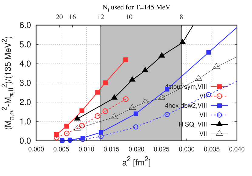
Figure 5: Taste breaking for our previous 4stout action with Symanzik-improved gauge sector (red), HotQCD’s HISQ action (black), and our new 4HEX action with DBW2 gauge sector (blue). The improvement in the taste breaking is evident.

Systematic analysis

In order to obtain the continuum extrapolations shown in Figs. 1, 2, we used the following ansatz:

$$\hat{O}(T,1/N_{\tau}^{2})=\sum_{i=1}^{M}\left(\alpha_{i}+\beta_{i}\frac{1}{N_{\tau}^{2}}\right)s_{i}(T)\,\,,$$ (5)

where the $s_{i}(T)$ are a set of basis spline functions. In order to take into account the ambiguity in the temperature definition, we employ settings of the scale with both $f_{\pi}$ and $w_{1}$, as previously mentioned, and include three different sets of node points to define the basis functions $s_{i}(T)$. The final results are obtained by combining the $6=2\times 3$ analyses to construct a histogram. The width of the histogram defines the systematic error. In the plots we show combined errors, where we assume that statistical and systematic errors add up in quadrature. This systematic error estimation procedure has been used and described in more detail in several of our works, most recently in Ref. [44].

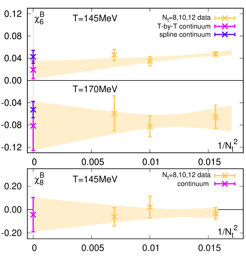
Figure 6: Continuum extrapolation of $\chi_{6}^{B}$ (top panel) at $T=145,170\,{\rm MeV}$ and $\chi_{8}^{B}$ (bottom panel) at $T=145\,{\rm MeV}$. For the different temperatures, the finite $N_{\tau}$ data are shown along with their continuum extrapolation. In the case of $\chi_{6}^{B}$, the results of the combined spline and continuum fit (depicted in Fig. 2), are also shown.

We show in Fig. 6 two example continuum extrapolations of $\chi_{6}^{B}$, at $T=145,170\,{\rm MeV}$, and the continuum extrapolation of $\chi_{8}^{B}$ at $T=145\,{\rm MeV}$. In all cases, one can appreciate the small cutoff dependence of these quantities. In the case of $\chi_{6}^{B}$, we show the continuum extrapolation in pink, together with the result of the spline + continuum fit with the ansatz described in the previous paragraph.

Strangeness Neutrality

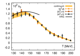
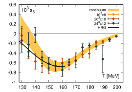
Figure 7: Our lattice results for the coefficients $s_{1}$ (left), $s_{3}$ (center), $s_{5}$ (right). The continuum extrapolation is shown as a yellow band. HRG model predictions are shown as solid black lines.

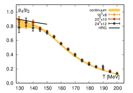
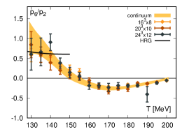
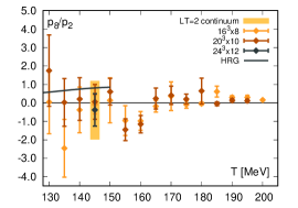
Figure 8: Our lattice results for the strangeness neutral ratios $p_{4}/p_{2}$ (left), $p_{6}/p_{2}$ (center), $p_{8}/p_{2}$ (right). For the first two, the continuum extrapolation is shown as a yellow band. HRG model predictions are shown as solid black lines.

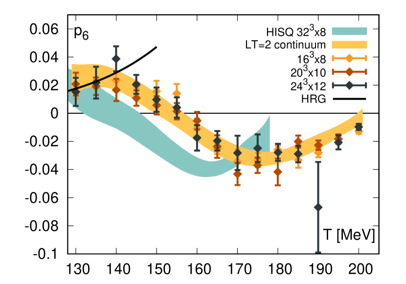
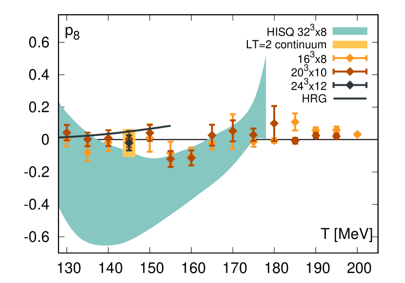
Figure 9: Our lattice results for the strangeness neutral fluctuations $p_{6}$ (top) and $p_{8}$ (bottom). The HISQ (splined) results are shown as light blue bands. Our new results for $p_{6}$ are shown as colored points for finite lattice spacing, and as a yellow band for the continuum. For $p_{8}^{B}$, our $N_{\tau}=8,10$ results are shown in different colors, together with the HISQ (splined) results.

In the main text we presented results for zero strangeness chemical potential $\mu_{S}=0$. A phenomenologically more relevant case is that of strangeness neutrality, where the strangeness chemical potential has to be tuned as a function of the baryochemical potential $\mu_{S}(\mu_{B})$ such that the expectation value for the strangeness density is zero $n_{S}\propto\frac{\partial p}{\partial\mu_{S}}=0$. This is done to every order in the Taylor expansion in $\mu_{B}$. The strangeness chemical potential itself is expanded as follows:

$$\mu_{S}(\mu_{B},T)=s_{1}(T)\left(\frac{\mu_{B}}{T}\right) +s_{3}(T)\left(\frac{\mu_{B}}{T}\right)^{3}$$ (6)

$$+s_{5}(T)\left(\frac{\mu_{B}}{T}\right)^{5}+\dots$$

where the coefficients $s_{1},s_{3}$ and $s_{5}$ are determined by solving $\frac{\partial p}{\partial\mu_{S}}=0$ order-by-order in the expansion parameter $\frac{\mu_{B}}{T}$. Our results for these coefficients are shown in Fig. 7. We also show the HRG predictions for these coefficients. We observe a good agreement for temperatures below $145$MeV.

Once these coefficients are known, we can also calculate the Taylor coefficients of the pressure on the strangeness neutral line:

$$p_{n}\equiv\left(\frac{\partial^{n}(p/T^{4})}{\partial(\mu_{B}/T)^{n}}\right)_{n_{S}=0}\rm.$$ (7)

Our results for the Taylor coefficient ratios $p_{4}/p_{2}$, $p_{6}/p_{2}$ and $p_{8}/p_{2}$ are shown in Fig. 8. We observe mild cut-off effects. Again, the HRG predictions are also shown.

We also show our results for $p_{6}$ and $p_{8}$ in Fig. 9. We show both the finite spacing results $16^{3}\times 8$, $20^{3}\times 10$ and $24^{3}\times 12$, as well as the continuum extrapolated results. Like in the main text, for the eith order coefficients $p_{8}$ the $24^{3}\times 12$ result, as well as the continuum extrapolated result is only available at a single temperature of $T=145$MeV. Our results are compared to results of the HotQCD collabotion using $32^{3}\times 8$ HISQ lattices from Ref. [6]. All conclusions are similar to the case of the coefficients $\chi^{B}_{6}$ and $\chi^{B}_{8}$, with the exception that unlike the case of $\chi^{B}_{6}$ and $\chi^{B}_{8}$, for the coefficients of $p_{6}$ and $p_{8}$ there are no results from the imaginary chemical potential method using the 4stout $48^{3}\times 12$ lattice action.

Statistics, parameters

$T$ [MeV]	$16^{3}\times 8$	$20^{3}\times 10$	$24^{3}\times 12$
130	31741	71090	68689
135	33528	106403	66960
140	34977	69690	75229
145	336975	188571	111435
150	65374	108481	81590
155	34057	96985	89559
160	37145	68619	94053
165	156044	67668	98744
170	34397	42314	11831
175	34180	36522	12089
180	30594	25229	12727
185	30951	18396	13066
190	30293	18267	7141
195	31276	15008	7199
200	31919	13346	7390

Table 1: Number of configurations analyzed on our three lattice geometries.

References

- Adamczyk et al. [2017] L. Adamczyk et al. (STAR), Bulk Properties of the Medium Produced in Relativistic Heavy-Ion Collisions from the Beam Energy Scan Program, Phys. Rev. C 96, 044904 (2017), arXiv:1701.07065 [nucl-ex] .
- Adam et al. [2021] J. Adam et al. (STAR), Nonmonotonic Energy Dependence of Net-Proton Number Fluctuations, Phys. Rev. Lett. 126, 092301 (2021), arXiv:2001.02852 [nucl-ex] .
- Bollweg et al. [2023] D. Bollweg, D. A. Clarke, J. Goswami, O. Kaczmarek, F. Karsch, S. Mukherjee, P. Petreczky, C. Schmidt, and S. Sharma (HotQCD), Equation of state and speed of sound of (2+1)-flavor QCD in strangeness-neutral matter at nonvanishing net baryon-number density, Phys. Rev. D 108, 014510 (2023), arXiv:2212.09043 [hep-lat] .
- Borsányi et al. [2021] S. Borsányi, Z. Fodor, J. N. Guenther, R. Kara, S. D. Katz, P. Parotto, A. Pásztor, C. Ratti, and K. K. Szabó, Lattice QCD equation of state at finite chemical potential from an alternative expansion scheme, Phys. Rev. Lett. 126, 232001 (2021), arXiv:2102.06660 [hep-lat] .
- Borsanyi et al. [2022] S. Borsanyi, J. N. Guenther, R. Kara, Z. Fodor, P. Parotto, A. Pasztor, C. Ratti, and K. K. Szabo, Resummed lattice QCD equation of state at finite baryon density: Strangeness neutrality and beyond, Phys. Rev. D 105, 114504 (2022), arXiv:2202.05574 [hep-lat] .
- Bollweg et al. [2022] D. Bollweg, J. Goswami, O. Kaczmarek, F. Karsch, S. Mukherjee, P. Petreczky, C. Schmidt, and P. Scior (HotQCD), Taylor expansions and Padé approximants for cumulants of conserved charge fluctuations at nonvanishing chemical potentials, Phys. Rev. D 105, 074511 (2022), arXiv:2202.09184 [hep-lat] .
- Aoki et al. [2006] Y. Aoki, G. Endrodi, Z. Fodor, S. D. Katz, and K. K. Szabo, The Order of the quantum chromodynamics transition predicted by the standard model of particle physics, Nature 443, 675 (2006), arXiv:hep-lat/0611014 .
- Kovács et al. [2016] P. Kovács, Z. Szép, and G. Wolf, Existence of the critical endpoint in the vector meson extended linear sigma model, Phys. Rev. D 93, 114014 (2016), arXiv:1601.05291 [hep-ph] .
- Critelli et al. [2017] R. Critelli, J. Noronha, J. Noronha-Hostler, I. Portillo, C. Ratti, and R. Rougemont, Critical point in the phase diagram of primordial quark-gluon matter from black hole physics, Phys. Rev. D 96, 096026 (2017), arXiv:1706.00455 [nucl-th] .
- Isserstedt et al. [2019] P. Isserstedt, M. Buballa, C. S. Fischer, and P. J. Gunkel, Baryon number fluctuations in the QCD phase diagram from Dyson-Schwinger equations, Phys. Rev. D 100, 074011 (2019), arXiv:1906.11644 [hep-ph] .
- Fu et al. [2021] W.-j. Fu, X. Luo, J. M. Pawlowski, F. Rennecke, R. Wen, and S. Yin, Hyper-order baryon number fluctuations at finite temperature and density, Phys. Rev. D 104, 094047 (2021), arXiv:2101.06035 [hep-ph] .
- Stephanov [2011] M. A. Stephanov, On the sign of kurtosis near the QCD critical point, Phys. Rev. Lett. 107, 052301 (2011), arXiv:1104.1627 [hep-ph] .
- Mroczek et al. [2021] D. Mroczek, A. R. Nava Acuna, J. Noronha-Hostler, P. Parotto, C. Ratti, and M. A. Stephanov, Quartic cumulant of baryon number in the presence of a QCD critical point, Phys. Rev. C 103, 034901 (2021), arXiv:2008.04022 [nucl-th] .
- Pisarski and Wilczek [1984] R. D. Pisarski and F. Wilczek, Remarks on the Chiral Phase Transition in Chromodynamics, Phys. Rev. D 29, 338 (1984).
- Ding et al. [2019] H. T. Ding et al. (HotQCD), Chiral Phase Transition Temperature in ( 2+1 )-Flavor QCD, Phys. Rev. Lett. 123, 062002 (2019), arXiv:1903.04801 [hep-lat] .
- Kotov et al. [2021] A. Y. Kotov, M. P. Lombardo, and A. Trunin, QCD transition at the physical point, and its scaling window from twisted mass Wilson fermions, Phys. Lett. B 823, 136749 (2021), arXiv:2105.09842 [hep-lat] .
- Almasi et al. [2017] G. A. Almasi, B. Friman, and K. Redlich, Baryon number fluctuations in chiral effective models and their phenomenological implications, Phys. Rev. D 96, 014027 (2017), arXiv:1703.05947 [hep-ph] .
- Bonati et al. [2015] C. Bonati, M. D’Elia, M. Mariti, M. Mesiti, F. Negro, and F. Sanfilippo, Curvature of the chiral pseudocritical line in QCD: Continuum extrapolated results, Phys. Rev. D 92, 054503 (2015), arXiv:1507.03571 [hep-lat] .
- Borsanyi et al. [2020] S. Borsanyi, Z. Fodor, J. N. Guenther, R. Kara, S. D. Katz, P. Parotto, A. Pasztor, C. Ratti, and K. K. Szabo, QCD Crossover at Finite Chemical Potential from Lattice Simulations, Phys. Rev. Lett. 125, 052001 (2020), arXiv:2002.02821 [hep-lat] .
- Yang and Lee [1952] C.-N. Yang and T. D. Lee, Statistical theory of equations of state and phase transitions. 1. Theory of condensation, Phys. Rev. 87, 404 (1952).
- Lee and Yang [1952] T. D. Lee and C.-N. Yang, Statistical theory of equations of state and phase transitions. 2. Lattice gas and Ising model, Phys. Rev. 87, 410 (1952).
- Giordano and Pásztor [2019] M. Giordano and A. Pásztor, Reliable estimation of the radius of convergence in finite density QCD, Phys. Rev. D 99, 114510 (2019), arXiv:1904.01974 [hep-lat] .
- Mukherjee and Skokov [2021] S. Mukherjee and V. Skokov, Universality driven analytic structure of the QCD crossover: radius of convergence in the baryon chemical potential, Phys. Rev. D 103, L071501 (2021), arXiv:1909.04639 [hep-ph] .
- Giordano et al. [2020] M. Giordano, K. Kapas, S. D. Katz, D. Nogradi, and A. Pasztor, Radius of convergence in lattice QCD at finite with rooted staggered fermions, Phys. Rev. D 101, 074511 (2020), [Erratum: Phys.Rev.D 104, 119901 (2021)], arXiv:1911.00043 [hep-lat] .
- Basar [2021] G. Basar, Universality, Lee-Yang Singularities, and Series Expansions, Phys. Rev. Lett. 127, 171603 (2021), arXiv:2105.08080 [hep-th] .
- Dimopoulos et al. [2022] P. Dimopoulos, L. Dini, F. Di Renzo, J. Goswami, G. Nicotra, C. Schmidt, S. Singh, K. Zambello, and F. Ziesché, Contribution to understanding the phase structure of strong interaction matter: Lee-Yang edge singularities from lattice QCD, Phys. Rev. D 105, 034513 (2022), arXiv:2110.15933 [hep-lat] .
- Majumder and Muller [2010] A. Majumder and B. Muller, Hadron Mass Spectrum from Lattice QCD, Phys. Rev. Lett. 105, 252002 (2010), arXiv:1008.1747 [hep-ph] .
- Bazavov et al. [2014] A. Bazavov et al., Additional Strange Hadrons from QCD Thermodynamics and Strangeness Freezeout in Heavy Ion Collisions, Phys. Rev. Lett. 113, 072001 (2014), arXiv:1404.6511 [hep-lat] .
- Alba et al. [2017] P. Alba et al., Constraining the hadronic spectrum through QCD thermodynamics on the lattice, Phys. Rev. D 96, 034517 (2017), arXiv:1702.01113 [hep-lat] .
- Workman et al. [2022] R. L. Workman et al. (Particle Data Group), Review of Particle Physics, PTEP 2022, 083C01 (2022).
- Bzdak et al. [2013] A. Bzdak, V. Koch, and V. Skokov, Baryon number conservation and the cumulants of the net proton distribution, Phys. Rev. C 87, 014901 (2013), arXiv:1203.4529 [hep-ph] .
- Braun-Munzinger et al. [2021] P. Braun-Munzinger, B. Friman, K. Redlich, A. Rustamov, and J. Stachel, Relativistic nuclear collisions: Establishing a non-critical baseline for fluctuation measurements, Nucl. Phys. A 1008, 122141 (2021), arXiv:2007.02463 [nucl-th] .
- Vovchenko et al. [2020] V. Vovchenko, O. Savchuk, R. V. Poberezhnyuk, M. I. Gorenstein, and V. Koch, Connecting fluctuation measurements in heavy-ion collisions with the grand-canonical susceptibilities, Phys. Lett. B 811, 135868 (2020), arXiv:2003.13905 [hep-ph] .
- Borsányi et al. [2012] S. Borsányi, G. Endrődi, Z. Fodor, S. Katz, S. Krieg, et al., QCD equation of state at nonzero chemical potential: continuum results with physical quark masses at order , JHEP 1208, 053, arXiv:1204.6710 [hep-lat] .
- Bellwied et al. [2015] R. Bellwied, S. Borsányi, Z. Fodor, S. D. Katz, A. Pásztor, C. Ratti, and K. K. Szabó, Fluctuations and correlations in high temperature QCD, Phys. Rev. D92, 114505 (2015), arXiv:1507.04627 [hep-lat] .
- Mogliacci et al. [2013] S. Mogliacci, J. O. Andersen, M. Strickland, N. Su, and A. Vuorinen, Equation of State of hot and dense QCD: Resummed perturbation theory confronts lattice data, JHEP 12, 055, arXiv:1307.8098 [hep-ph] .
- Haque et al. [2014] N. Haque, J. O. Andersen, M. G. Mustafa, M. Strickland, and N. Su, Three-loop pressure and susceptibility at finite temperature and density from hard-thermal-loop perturbation theory, Phys. Rev. D 89, 061701 (2014), arXiv:1309.3968 [hep-ph] .
- Bazavov et al. [2020] A. Bazavov et al., Skewness, kurtosis, and the fifth and sixth order cumulants of net baryon-number distributions from lattice QCD confront high-statistics STAR data, Phys. Rev. D 101, 074502 (2020), arXiv:2001.08530 [hep-lat] .
- Sharpe [2006] S. R. Sharpe, Rooted staggered fermions: Good, bad or ugly?, PoS LAT2006, 022 (2006), arXiv:hep-lat/0610094 .
- Bazavov et al. [2010] A. Bazavov et al. (MILC), Nonperturbative QCD Simulations with 2+1 Flavors of Improved Staggered Quarks, Rev. Mod. Phys. 82, 1349 (2010), arXiv:0903.3598 [hep-lat] .
- Borsanyi et al. [2010] S. Borsanyi, Z. Fodor, C. Hoelbling, S. D. Katz, S. Krieg, C. Ratti, and K. K. Szabo (Wuppertal-Budapest), Is there still any mystery in lattice QCD? Results with physical masses in the continuum limit III, JHEP 09, 073, arXiv:1005.3508 [hep-lat] .
- D’Elia et al. [2017] M. D’Elia, G. Gagliardi, and F. Sanfilippo, Higher order quark number fluctuations via imaginary chemical potentials in QCD, Phys. Rev. D 95, 094503 (2017), arXiv:1611.08285 [hep-lat] .
- Borsanyi et al. [2016] S. Borsanyi et al., Calculation of the axion mass based on high-temperature lattice quantum chromodynamics, Nature 539, 69 (2016), arXiv:1606.07494 [hep-lat] .
- Borsányi et al. [2018] S. Borsányi, Z. Fodor, J. N. Günther, S. K. Katz, K. K. Szabó, A. Pásztor, I. Portillo, and C. Ratti, Higher order fluctuations and correlations of conserved charges from lattice QCD, JHEP 10, 205, arXiv:1805.04445 [hep-lat] .
- Follana et al. [2007] E. Follana, Q. Mason, C. Davies, K. Hornbostel, G. P. Lepage, J. Shigemitsu, H. Trottier, and K. Wong (HPQCD, UKQCD), Highly improved staggered quarks on the lattice, with applications to charm physics, Phys. Rev. D 75, 054502 (2007), arXiv:hep-lat/0610092 .
- Hasenfratz and Karsch [1983] P. Hasenfratz and F. Karsch, Chemical Potential on the Lattice, Phys. Lett. B 125, 308 (1983).
- Roberge and Weiss [1986] A. Roberge and N. Weiss, Gauge Theories With Imaginary Chemical Potential and the Phases of QCD, Nucl. Phys. B 275, 734 (1986).
- Capitani et al. [2006] S. Capitani, S. Durr, and C. Hoelbling, Rationale for UV-filtered clover fermions, JHEP 11, 028, arXiv:hep-lat/0607006 .
- de Forcrand et al. [1998] P. de Forcrand et al. (QCD-TARO), Renormalization group flow of SU(3) gauge theory, (1998), arXiv:hep-lat/9806008 .
- Borsanyi et al. [2023a] S. Borsanyi, Z. Fodor, M. Giordano, J. N. Guenther, S. D. Katz, A. Pasztor, and C. H. Wong, Equation of state of a hot-and-dense quark gluon plasma: Lattice simulations at real B vs extrapolations, Phys. Rev. D 107, L091503 (2023a), arXiv:2208.05398 [hep-lat] .
- Borsanyi et al. [2023b] S. Borsanyi, Z. Fodor, M. Giordano, J. N. Guenther, S. D. Katz, A. Pasztor, and C. H. Wong, Can rooted staggered fermions describe nonzero baryon density at low temperatures?, (2023b), arXiv:2308.06105 [hep-lat] .
- Allton et al. [2002] C. R. Allton, S. Ejiri, S. J. Hands, O. Kaczmarek, F. Karsch, E. Laermann, C. Schmidt, and L. Scorzato, The QCD thermal phase transition in the presence of a small chemical potential, Phys. Rev. D66, 074507 (2002), arXiv:hep-lat/0204010 [hep-lat] .
- Aoki et al. [2014] S. Aoki et al., Review of Lattice Results Concerning Low-Energy Particle Physics, Eur. Phys. J. C 74, 2890 (2014), arXiv:1310.8555 [hep-lat] .
- Colangelo and Durr [2004] G. Colangelo and S. Durr, The Pion mass in finite volume, Eur. Phys. J. C 33, 543 (2004), arXiv:hep-lat/0311023 .
- Borsanyi et al. [2012] S. Borsanyi et al., High-precision scale setting in lattice QCD, JHEP 09, 010, arXiv:1203.4469 [hep-lat] .