A cosmological “Big Storm Scenario"
following the QCD phase transition

Abstract

It was proposed that acoustic perturbations generated by the QCD phase transition could create an inverse turbulent cascade Kalaydzhyan and Shuryak (2015). An assumption was that propagation toward smaller momenta could reach the wavelength of a few km, the Universe’s size at the time. Such acoustic waves were proposed to be the source of gravity waves. The kilometer wavelength corresponds to year-long gravity wave today, which were recently discovered using pulsar correlations.

This paper argues further that an acoustic turbulence must be an ensemble of shocks. This brings two consequences: First, shocks generate gravity waves much more efficiently than sound waves due to the intermittency of matter distribution. We reconsider gravity wave radiation, using universal emission theory for soft radiation, and argue that soft-momenta plateau should reach wavelengths of the order of shock mean free paths. Second, collisions of shock waves create local density excess, which may create primordial black holes. A good tool to settle this issue can be an evaluation of the trapped surfaces like it was done in studies of heavy ion collisions using AdS/CFT correspondence.

I Introduction

The time of the cosmological phase transition follows from the standard Friedmann solution for radiation-dominated expansion

$$t_{QCD}=\big{(}{90\over 32\pi^{3}N_{DOF}}\big{)}^{1/2}{M_{P}\over T_{QCD}^{2}}$$ (1)

where $M_{P}=(\hbar c/G_{N})^{1/2}$ is the Plank mass, corresponding temperature is $T_{QCD}\approx 155\,MeV$ and $N_{DOF}$ is the effective number of bosonic degrees of freedom. The corresponding length scale is

$$h_{QCD}\sim c\cdot t_{QCD}\sim 10\,km$$ (2)

The scenario to be discussed originates from paper Kalaydzhyan and Shuryak (2015) which can be briefly summarized as follows.
(i) Disturbances created at the cosmological QCD phase transitions produce sound waves originating at the (UV) scale $k\sim T_{c}$ ;
(ii) Subsequent acoustic turbulence enters an inverse cascade regime and as a result amplitude of sounds $n_{k}$ increases as they propagate toward small momenta, $k\rightarrow 1/h_{QCD}$. The amplitudes of the waves increase, thus the storm. The wavelength $h_{QCD}$ is multiplied by corresponding Universe expansion $z$ factor and constitute about one light year today.
(iii) The production of gravitational waves was described by the elementary process two sound waves -> gravity wave (GW).

In the intervening years, several experimental discoveries and theoretical developments provided new reasons to focus on the Universe at the scale $h_{QCD}$. As usual, new developments lead to many interesting questions and problems. We will briefly review some of them below, which could be useful, as they touch on quite different fields of physics.

In the intervening years, the most important for the subject in question is that GW with period $\sim 1\,year$ were in fact observed. Several Pulsar Timing Array groups have reported the discovery of a stochastic gravitational wave background (SGWB). In particular, the North American Nanohertz Observatory for Gravitational Waves (NANOGrav) Agazie et al. (2023), the European PTA Antoniadis et al. (2023), the Parkes PTA Reardon et al. (2023) and the Chinese CPTA Xu et al. (2023) have all released results which seem to be consistent with expected pattern in the angular correlations characteristic of the SGWB. If these GW are of cosmological origin, one now gets the absolute scale of their amplitude at $t_{QCD}$, which can be compared to proposed mechanisms of their radiation.

In this paper, we reconsider and significantly change the scenario, taking into account the fact that acoustic waves of finite amplitude in a medium with a low viscosity inevitably turn into shocks.

We also propose that density perturbations induced by storms in cosmological settings may create, under certain conditions, “overdense" regions to undergo gravitational collapse, generating “primordial black holes", PBHs. Well-known studies of the phenomenon were all done in spherically symmetric density fluctuations in a standard expanding Universe. Studies of colliding shocks were done in a completely different field of physics, describing ultrarelativistic heavy ion collisions via AdS/CFT correspondence. BH formation has been studied by calculating trapped surfaces. There, general relativity was used in higher dimensions, as dual to QCD, but methodically it is very close to what we need. This theory can easily be modified to address the collapse in the standard General Relativity. An important tool used in those papers is evaluating the trapped surfaces, providing lower bounds on BH masses.

II Soft graviton emission without a storm

Let us start with a discussion of why there can be sounds after the phase transitions, and whether they can go into a turbulent regime.

QCD phase transition has been studied experimentally in heavy ion collisions, in the last decades, mostly at two colliders, RHIC at Brookhaven National Laboratory, USA and LHC at CERN. They study the transition of matter from the Quark-Gluon Plasma (QGP) phase to Hadron Resonance Gas (HRG). Relevant for our discussion are studies of sound excitations. This is done via the so called azimuthal harmonics of the flow $v_{m}$ with the range $m=2...10$. They are sounds with the wavelength $\lambda_{m}=2\pi R_{fireball}/m$, ranging from $20$ to $4\,fm$. Their amplitudes depend on sound velocity $c_{s}=dp/d\rho\approx 0.16$. Their damping reveals surprisingly low viscosity of the plasma.

Naively, one may expect that the Universe expansion is rather slow, with the system having more than enough time to adjust to changing temperature $T(t)$ and be near thermal equilibrium. The phase transitions are still expected to produce perhaps certain out-of-equilibrium excitations: the first-order transitions with its bubbles is the best-known example. “Critical opalescence" while passing the second-order transitions is another well-known example. (A search for such a hypothetical QCD critical point is an experimental program at RHIC, so far without a widely accepted conclusion.) Small but finite quark masses smoothed the (chiral symmetry breaking) QCD transition at $T_{c}$, believed to be just a crossover. Yet, even for such a regime, one may expect an inhomogeneous distribution of both phases. One particular model has been discussed in Shuryak and Staig (2013): instead of slowly evaporating, the QGP clusters should undergo collapse, transferring (part of) their energy/entropy into the outgoing sounds. Instead of bubble collisions, they individually participate in spherical collapse, as has been demonstrated for bubbles in water by Rayleigh. If so, most sounds is emitted at wavelength corresponding to the smallest size of the collapsing QGP cluster, perhaps again at the micro or UV scale $1/T_{c}$.

In Kalaydzhyan and Shuryak (2015), it was proposed that the collision of sound waves can be the origin of GWs. Considering sound momenta $\vec{p}_{1},\vec{p}_{2}$ and $\vec{q}$ of the GW to be comparable, it was argued for a peak in the emission spectrum Kalaydzhyan and Shuryak (2015). In this work we will focus instead on soft gravitons, with $q\ll p_{1},p_{2}$.

The emission of soft gravitons, like that of soft photons, follow particle collisions in universal factorized form pointed out by Weinberg Weinberg (1965), with extra factors in each line of the Feynman diagram being

$$f_{photons} = \sum_{n}{e_{n}\eta_{n}p_{n}^{\mu}\over(pq)-i\epsilon\eta_{n}}$$ (3)

$$f_{gravitons} = (8\pi G_{N})^{1/2}\sum_{n}{\eta_{n}p_{n}^{\mu}p_{n}^{\mu}\over(pq)-i\epsilon\eta_{n}}$$

where $\eta_{n}=1$ for outgoing lines and $-1$ for in-going ones, $p^{\mu},q^{\mu}$ are momenta of the parent particle and GW, respectively. The emission cross-sections are singular at $q\rightarrow 0$, but only because they count a number of photons/gravitons. To give the power spectrum, the cross sections need to be multiplied by the energy $q_{0}=\hbar\omega$, then $\hbar$ cancels out in the dimensionless factors such as

$${G_{N}M_{N}^{2}\over\hbar c}\approx 5.8\cdot 10^{-39}$$ (4)

(with $M_{N}$ here being the nucleon’s mass). The resulting expressions for power production has no $\hbar$, so they are valid in both quantum and classical domains.

Note that Weinberg’s calculation contains the transport cross-section $\sigma_{t}$, namely the one weighted with the momentum transfer. Let us explain why this is the case. The emitter of soft gravity waves summing over incoming and outgoing lines for $2\rightarrow 2$ collisions reads

$$- p_{1,in}^{\mu}p_{1,in}^{\nu}-p_{2,in}^{\mu}p_{2,in}^{\nu}+p_{1,out}^{\mu}p_{1,out}^{\nu}+p_{1,out}^{\mu}p_{1,out}^{\nu}$$ (5)

$$= p_{1,out}^{\mu}p_{2,out}^{\nu}-p_{1,in}^{\mu}p_{2,in}^{\nu}+(\mu\leftrightarrow\nu)$$

where the second line is obtained using momentum conservation $p_{1,in}^{\mu}+p_{2,in}^{\mu}=p_{1,out}^{\mu}+p_{2,out}^{\mu}$. It vanishes for forward scattering, $p_{1,in}=p_{1,out},p_{2,in}=p_{2,out}$. So, there is no soft GW radiation without a change in the stress tensor $T^{\mu\nu}$.

For nonrelativistic collisions producing gravitons with energy below $\Lambda$, Weinberg calculated the total power emitted via soft gravitons to be

$$P(q_{0}<\Lambda)={8G_{N}\Lambda\over 5\pi}m^{2}v^{5}n_{a}n_{b}\sigma_{transport}V$$ (6)

where $n_{a},n_{b}$ are densities of colliding particles, $V$ is interacting volume, $v$ velocity and $\sigma_{transport}$ is the transport cross section (weighted with $sin(\theta)^{2}$). As an exercise, for electron-proton collisions in the Sun, he estimated this power. Substituting regulated cross section one gets the power of the Sun about $P_{Sun\,gravitons}\approx 70MW$ emitted in sub-$keV$ gravitons.

For comparison, total Sun power in thermal photons is $P_{Sun}=4.4\cdot 10^{16}Watts$. A reader may wonder why GW radiation is only billion times smaller than electromagnetic one, in spite of the fact that its coupling is smaller by about 38 orders of magnitude? Without going into complicated nuclear physics of the Sun energy production, let us just note one effect: soft photons are emitted into a heat bath in thermal equilibrium, so their emission must be balanced by photon absorption. GWs, on the other hand, are never close to thermal equilibrium, inverse reactions are negligible and their radiation proceeds unobstructed as estimated.

Following this reasoning, let us evaluate the production of soft gravitons accompanying hadronic collisions in hadron resonance gas before/after the QCD phase transition. In the plasma phase, effective masses of quark and gluon quasiparticles are $O(1\,GeV)$. Most hadronic species in HRG have the same order of magnitude. Comparing to typical thermal momenta $3T_{QCD}\sim 0.5\,GeV$ one may take the nonrelativistic estimate as qualitatively valid. With $M=1\,GeV,n_{a}=n_{b}=1/fm^{3},V=1\cdot m^{3}$ we estimate soft graviton power production to be

$$P_{HRG}\sim 6\cdot 10^{18}kg/m/s^{3}$$

The energy produced during time $t_{QCD}\sim 10^{-5}s$ gives the energy density (per $m^{3}$)

$$\rho_{gravitons}\sim 1.6\cdot 10^{24}{kg\over ms^{2}}$$

For comparison, the energy density of matter itself is

$$\rho_{matter}\sim 1\,GeV/fm^{3}\sim 1.6\cdot 10^{35}{kg\over ms^{2}}$$

eleven orders of magnitude larger. A very small radiation rate, containing a very small dimensionless ratio (4), is compensated by the relatively long duration of the emission time (the QCD era): gravitons, unlike photons and strongly interacting species, are only emitted, with negligible absorption. This type of enhancement of any “penetrating probe" production is well known in the heavy-ion collision community, among others.

A more formal answer to the question of why it is not suppressed much more can be given as follows: since the duration $t_{QCD}$ (1) is proportional to the Plank mass $M_{P}=\sqrt{\hbar\cdot c/G_{N}}$, the energy density of the soft GW produced is in fact proportional to a square root $\sqrt{G_{N}}$, not small coupling $G_{N}$ itself.

There are recent studies of soft graviton production from cosmological perturbations Sharma et al. (2023). These authors did find a universal “shallow relic" of the acoustic peak at small momenta, but that has an energy spectrum linear in momentum $\Omega_{GW}\sim k$. Their model is very different from soft radiation from particle collisions considered above, and thus, there is no contradiction between these results.

It is convenient to convert the observed radiation in energy density units at the current time to the time $t_{QCD}$. If this radiation is primordial, its energy density scales as $z^{4}$. The corresponding factor $z_{QCD}=T_{QCD}/T_{now}\approx 6\cdot 10^{11}$. Using observed

$$\rho_{GW\,now}\approx 7.1\cdot 10^{-17}{kg\over ms^{2}}$$ (7)

we get

$$\rho_{GW\,QCD}\approx 9\cdot 10^{30}{kg\over ms^{2}}$$ (8)

This is of the order of $10^{-5}$ of matter density, but also six orders of magnitude larger than due to soft graviton emission evaluated above.

III Acoustic turbulence as an ensemble of (relativistic) shocks

The turbulence of acoustic waves in a medium with sufficiently low viscosity is a set of shock waves, see e.g. Fig.1 taken from the recent paper Kochurin, E.A. and Kuznetsov,E.A (2022).

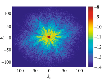
Figure 1: The energy spectrum $E_{\vec{k}}$ in momentum space. The peaks correspond to “pancake-shaped" shock waves. Their height is $\sim 1/d$, and the width $\sim 1/R$, where $d,R$ are the width and radius of these pancakes.

In our case of QGP/hadronic gas, the velocity of even weak shocks coincides with the speed of sound $c_{s}=c/\sqrt{3}\approx 0.55\cdot c$, comparable to the speed of light. Stronger shocks move even with a larger speed. Therefore, one must use relativistic notations, so we explain those first. Hydrodynamics is described by motion of matter defined via (Lorentz scalars) energy density $\rho$ and pressure $p$, and the collective flow velocity. It is promoted to 4-vector $u^{\mu},\mu=0,1,2,3$ making the stress tensor in local approximation (zero viscosity) as

$$T_{\mu\nu}=(\rho+p)u^{\mu}u^{\nu}+pg^{\mu\nu}$$ (9)

Even if the motion happens in one dimension, there are two components of 4-velocity $u^{0},u^{1}$, constrained by $(u^{0})^{2}-(u^{1})^{2}=1$. Using $u^{0}=cosh(y),u^{1}=sinh(y)$ one uses a parameter $y$ called $rapidity$. Unlike velocity, its Lorentz transformation is done by simple additive shift.

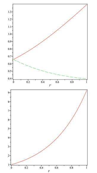
Figure 2: (Upper plot) The rapidity of the shock $y$ versus the matter rapidity $Y$ is shown by upper (red) solid line, while the lower (green) dashed line shows rapidity of another side $y-Y$. (Lower plot) The compression ratio of matter versus $Y$ .

The shock relations are given by continuity of energy and momentum flow. Omitting details (see Shuryak (2012)) we explain the setting and results. Consider relativistic matter moving with rapidity $y$ and undergoing energy density jump at a shock moving with rapidity $Y$. After becoming compressed, the matter has rapidity $y-Y$. The solution of the continuity equations is as follows:

$$y(Y)=Y-{1\over 2}log\big{(}e^{2Y}+1-\sqrt{e^{4Y}+e^{2Y}+1}\big{)}\,.$$ (10)

Fig.2 shows the relation for a relativistic fluid ($p=\rho/3$). As you can see when the shock is weak ($Y\approx 0$), matter compression is small, and its speed is that of the sound $y=tanh(c_{s})=tanh(\sqrt{1/3})$.

With increasing $Y$ the compression contrast between upstream and downstream matter grows, reaching about an order of magnitude for $Y\sim 1$. Even for more realistic $Y\approx 1/2$, the shock rapidity $y_{shock}\approx 1$ and velocity $v_{shock}=tanh(y)\approx 0.76$, and compression is already $\sim 2.5$.

The paper is Shuryak (2012) mostly devoted to calculation of the profile of strong shocks in strongly coupled plasma, using AdS/CFT correspondence. It may be used for more detailed studies of shock collisions and GW radiation, but not it is not used in the present paper and thus not discussed.

IV Gravity wave emission from shock ensemble

Standard approaches to GW emission are based on the correlator of two stress tensors. For an emission by sound waves of small amplitude, the terms $(\rho+p)u^{\mu}u^{\nu}$ are expanded in the wave amplitudes. Since the velocity is of the first order, $(\rho+p)$ is taken in the zeroth order. The correlators of velocities are usually calculated assuming an independent Gaussian ensemble of waves. The mean power of gravity waves emitted by sound is proportional to the mean squared power of acoustic waves, which was estimated as the squared mean power.

Such estimates are off by a large factor for a highly intermittent set of shock waves. Indeed, for a set of locally plane shocks, one can use the Burgers scaling for the moments of the velocity difference $\delta v$ taken at the distance $l$: $\langle(\delta\vec{v})^{n}\rangle\simeq v_{rms}^{n}l/L$, where $L$ is the mean distance between shocks. That gives the fourth moment of the velocity difference strongly enhanced in comparison with the squared second moment

$$\langle(\delta\vec{v})^{4}\rangle\simeq\langle(\delta\vec{v})^{2}\rangle^{2}{L\over l}\,.$$ (11)

The largest enhancement is for $l\simeq d$, where $d$ is the width of the shock front. Furthermore, in strong turbulence with shocks, there is no small-amplitude expansion since $\delta(\rho+p)$ and 4-velocities $u^{\mu}$ are not small but rather $O(1)$.

Both nonrelativistic and relativistic shocks have the same characteristic feature: stronger ones move quicker, catching and absorbing weaker ones so shock turbulence gets stronger with time. So, suppose the main events happening are $2\rightarrow 1$ processes. Let momentum conservation be expressed as $p_{1}^{\mu}+p_{2}^{\mu}=P^{\mu}$. The soft gravitons are then emitted by the stress tensor change

$$\delta T^{\mu\nu} = P^{\mu}P^{\nu}-p_{1}^{\mu}p_{1}^{\nu}-p_{2}^{\mu}p_{2}^{\nu}$$ (12)

$$= p_{1}^{\mu}p_{2}^{\nu}+p_{1}^{\nu}p_{2}^{\mu}$$

which in this case is always nonzero. Therefore emission rate should include the ordinary cross-section (rather than the transport one, as was the case for the $2\rightarrow 2$ scattering).

Let us now clarify the following question: How can soft gravitons be emitted at large times/distances between shock collisions when they do not yet overlap? Let us start answering it with soft photons. While a charged particle can be well localized on its trajectory, its e/m field cannot. In particular, at rest, it is a Coulomb field $A_{0}\sim e/r$.

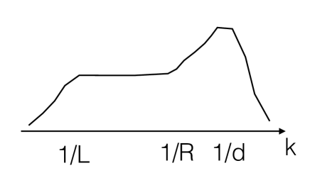
Figure 3: Schematic shape of the GW energy spectrum emitted by shock ensemble. For the meaning of the indicated parameters, see text.

If objects are locally flat “pancakes", the transverse size $R$ is much larger than the width $d$. Face-to-face collisions will have the shortest duration $t_{face-to-face}\sim d/cosh(Y)$ ($Y$ is shock rapidity, cosh gives compression by the Lorentz factor). Collisions of “pancakes" with nonzero angles last longer, all the way to orthogonal collisions with $t_{angle}\propto R$. Radiation emitted would have an asymmetric peak at the corresponding frequencies, ranging from $1/t_{face-to-face}$ to $1/R$. A schematic picture of the gravity wave spectrum is shown in Fig.3. Explicit calculations for various models of turbulence after the phase transitions (such as Sharma et al. (2023)) lead to similar shapes.

We suggest that a “universal shoulder" in the spectrum toward the IR appears due to the emission of soft gravitons. As we discussed above, it is due to general expressions for soft emissions from collision processes in which the stress tensor suffers rapid changes. An important question is how far the soft GW shoulder reaches toward small $k$. Note that their emission happens during the time between collisions. As pointed out by Feinberg and Pomeranchuk in 1950’s, after each scattering, the electron appears “semi-naked", with a reduced electric field, which gradually regenerates later. Obviously, the same should be true for soft GW.

If shocks move relativistically, with Lorentz factor significantly larger than 1, their gravity field also gets Lorentz contracted into a pancake. When they change velocity or direction of motion, part of their Newtonian field continues into the old direction, constituting the soft radiation we discuss. We, therefore, state that the universal shoulder should reach the mean free path of the radiated objects. For the ensemble of shocks this longest time scale is

$$L\sim{1\over n\sigma v}\sim{1\over n_{shocks}(4\pi R^{2})}$$ (13)

Furthermore, since we are aiming to explain the observed GW background with periods $\sim 1$ year today, or $\lambda\sim ct_{QCD}\sim km$, then the left end of this shoulder should reach this scale, which is many orders larger than the microscopic scales defined by the ambient temperature $\lambda\sim 1/T_{QCD}$, with quasiparticle/hadrons mean free paths perhaps one or two orders of magnitude longer. Our proposal is that the strong turbulence leading to a picture of a rather dilute ensemble of shocks may eventually reach this scale. This implies that the shock density must be smaller than

$$n_{shocks}<{1\over c\cdot t_{QCD}\cdot(4\pi R^{2})}$$ (14)

where, we remind, $R$ is the transverse size of shock “pancakes".

V Primordial black holes from shock collisions?

Relativity and astronomy textbooks explain how BH may be produced in conventional stellar collapse. For decades, astronomers observed Supernovae without apparently nothing visible left at the center. Nowadays, after the LIGO/VERGO collaboration Ricci (2022) have observed BH mergers, they start getting some clues about BH mass spectrum. A significant surprise from the first event is that it is not easy to explain how BH with masses $M_{BH}\sim 20-30\,M_{Sun}$ were produced.

People wondered if those could be primordial ones (PBHs). Unfortunately, very little is known about the mass/spin distribution of BHs. The first observation of isolated BH nearby was recently detected by microlensing Sahu et al. (2022). Its mass is about $7\,M_{Sun}$, so it can well be of stellar origin. Interesting that distance is close enough to use the classical parallax method: so perhaps their density is rather high.

In principle, one may be able to tell primordial black holes (PBHs) from those created in stellar collapse by different momentum and spin distributions. Stellar BHs are expected to have large momentum due to “natal kicks" from supernovae, producing distinct distribution in Galaxy gravity field, e.g. be somewhat away from the Galaxy plane in which stars are. Perhaps with time, more will be found, and some ideas about their masses and space distribution of BHs will be clarified.

The idea that energy density fluctuations in the early Universe can lead to PBH originated by Zeldovich and Novikov Novikov and Zeldovich (1965) and then Hawking and especially Carr, see e.g. Carr (1975). While involved in Universe expansion, such matter as QGP or hadron resonance gas has pressure large enough to withstand gravitational instabilities. Yet, if some subvolume happens to have sufficient excess density, it may collapse. Early estimates Carr (1975) of the critical values

$${\delta\rho\over\rho}>\delta_{c}\sim c_{s}^{2}={dp\over d\rho}$$ (15)

needed for that relate it to the speed of sound. Near the QCD transition temperature, $c_{s}$ has a minimum known in heavy ion physics as “the softest point" of the equation of state. It was studied hydrodynamically Hung and Shuryak (1995) and then experimentally observed via a peak in the fireball lifetime as a function of the collision energy of heavy ions. Therefore, a minimum in the speed of sound, located in the vicinity of the QCD phase transition, should be suspected location for gravitational collapse. It is straightforward to estimate BHs masses produced, as they should contain all matter in a cell of size (2). This leads to

$$M_{PBH}\sim 20\,M_{Sun}$$

which is exactly in the ballpark of puzzling BHs seen by LIGO in mergers. Whether PBHs can or cannot be a significant fraction of the em dark matter is a hotly debated subject. Let us just comment that even if it is, than PBHs matter fraction at the QCD transition time should be of the order of only $\sim 10^{-9}$.

Multiple numerical solutions of Einstein’s equations has been made over the years to detail the process. As an example, consider Musco et al. (2005) and references therein. As in other works, spherical symmetry was assumed, with bulk matter flowing according to the usual (radiation-dominated) Friedmann solution. If density is supercritical, with time, one finds matter cells with positive and negative (directed inside) radial velocities, separated by a “void". (An interesting “second falling shell of matter" was also observed in these calculations.) The critical density contrast was found to be $\delta_{c}=\delta\rho/\rho\sim 0.43-0.47$. If density just slightly exceeds it, the mass of the produced PBS gets to be much smaller

$${M_{PBH}\over M_{H}}\sim(\delta-\delta_{c})^{\gamma}$$ (16)

traced over several orders of magnitude toward $10^{-4}$ or so, with the index $\gamma\approx 0.36$. An interesting option, then, is to search for BHs with masses $smaller$ than star collapse can generate. So far, none of such have been seen in mergers. In fact, there seems to be an empty gap in the LIGO data, between 2 and 5 $M_{Sun}$.

Returning to the scenario under consideration, one may ask if colliding shocks may provide strong enough density perturbation for a gravitational collapse. While locally the shocks themselves include significant matter compression, their sizes still are expected to be much smaller than visible size of the Universe, $d,R\ll c\cdot t_{QCD}$. On the other hand, their collisions include matter going toward the center with relativistic rapidities, which undoubtedly helps to initiate the gravitational collapse. Corresponding calculations can be done by simulating Einstein equation in such geometry, which is a task for subsequent works.

Ultrarelativistic collisions of shock-like objects in the hydrodynamical framework were pioneered by Landau Landau (1953), who applied hydrodynamics to ultrarelativistic collisions of hadrons and nuclei. Due to Lorentz contraction, those look like “pancakes of matter". While considered crazy at the time, it does described well the first rapidity distributions from colliders in 1970’s Shuryak (1972). Now it is proven that relativistic hydrodynamics does provide quantitative description of heavy ion collisions, in many details see e.g. Shuryak (2017).

A revival of studies of ultrarelativistic collisions happened in the framework of AdS/CFT holographic correspondence, relating certain strongly coupled gauge theories to string theories in higher dimensions. In the so called Maldacena limit, the latter basically being the Einstein’s general relativity in 5 dimensions. Such correspondence reproduces many observed features of Quark-Gluon Plasma (QGP) including the equation of state and viscosity. Ultrarelativistic collisions of shock-like objects were studied numerically and analytically, see e.g. Chesler and Yaffe (2011) and subsequent literature.

We want to emphasize one aspect of such calculations clarifying the production of the BHs in shock collisions. When colliding objects are about to overlap for the first time, so that the nontrivial solution of Einstein equations has not yet started, one can already study if the so-called trapped surface (for massless particles) may or may not be formed. If it does, its area provides the lower bound for the BH entropy. This tool was suggested by Gubser and used in several publications a decade ago. Most interesting feature of the trapped surface (found numerically by one of us in Lin and Shuryak (2009) and demonstrated in Fig.4 from Gubser et al. (2009)) is sharp disappearence of the trapped surface. Shown in the figure is the trapped surface $area$ as a function of the impact parameter. At a critical value of the impact parameter, the trapped surface disappears, while the area is still nonzero. That implies that the mass distribution of produced BHs may have a qute sharp cutoff at some minimal value.

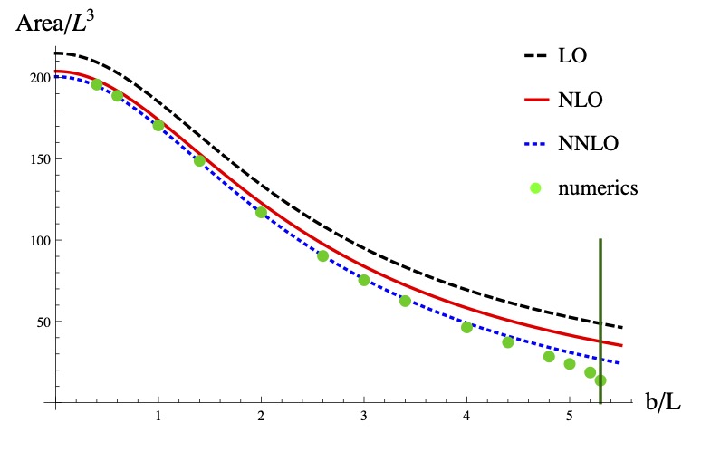
Figure 4: Area of trapped surface – the lower bound on the entropy of produced black hole – as a function of impact parameter. Curves are for different approximations developed in Gubser et al. (2009), and green points are from earlier numerical solutions in Lin and Shuryak (2009). Vertical line at the right side shows the impact parameter at which trapped surface disappears, indicating that BH production stops sharply at finite $b$.

VI Summary

We have proposed a “Big Storm Scenario" of what $may$ happen after the cosmological QCD phase transition. The main new idea introduced here is that the transition produces acoustic turbulence, which naturally becomes an ensemble of colliding shocks absorbing each other, getting stronger and more dilute with time.

We discuss the mechanism of the soft graviton production from shock collisions. Specifically, we focus on the smallest momenta, related to mean free paths of these shocks, which may reach the most interesting $km$ scale. If so, it may be the origin of the recently observed stochastic gravitational wave background of roughly a year period. Another intriguing issue is whether these shock collisions can seed the Universe with primordial black holes.

Many aspects of our scenario are hypothetical and suggested by and analogy to phenomena in related but different settings. Yet it is mostly based on “known physics". Many assumptions made can be clarified, by well-defined numerical simulations. The properties of shock distributions can be found, and the details of black hole production in shock collisions can be studied. We do understand EOS and many other properties of matter under consideration from heavy ion experiments. One cannot say that about alternative scenarios based on hypothetical fluctuations of the inflation process.

Acknowledgements We dedicate this paper to the memory of Vladimir E. Zakharov, a teacher, friend, and a giant of the theory of turbulence, who recently left us.
The work of ES is supported by the Office of Science, U.S. Department of Energy under Contract No. DE-FG-88ER40388. The work of GF was supported by the Excellence Center at WIS, by the grants 662962 and 617006 of the Simons Foundation, and by the EU Horizon 2020 programme under the Marie Sklodowska-Curie grant agreements No 873028 and 823937. GF thanks for hospitality the Simons Center for Geometry and Physics at Stony Brook.

References

- Kalaydzhyan and Shuryak (2015) T. Kalaydzhyan and E. Shuryak, Phys. Rev. D 91, 083502 (2015), arXiv:1412.5147 [hep-ph] .
- Agazie et al. (2023) G. Agazie et al. (NANOGrav), Astrophys. J. Lett. 951, L8 (2023), arXiv:2306.16213 [astro-ph.HE] .
- Antoniadis et al. (2023) J. Antoniadis et al. (EPTA), Astron. Astrophys. 678, A50 (2023), arXiv:2306.16214 [astro-ph.HE] .
- Reardon et al. (2023) D. J. Reardon et al., Astrophys. J. Lett. 951, L6 (2023), arXiv:2306.16215 [astro-ph.HE] .
- Xu et al. (2023) H. Xu et al., Res. Astron. Astrophys. 23, 075024 (2023), arXiv:2306.16216 [astro-ph.HE] .
- Shuryak and Staig (2013) E. Shuryak and P. Staig, Phys. Rev. C 88, 064905 (2013), arXiv:1306.2938 [nucl-th] .
- Weinberg (1965) S. Weinberg, Phys. Rev. 140, B516 (1965).
- Sharma et al. (2023) R. Sharma, J. Dahl, A. Brandenburg, and M. Hindmarsh, (2023), arXiv:2308.12916 [gr-qc] .
- Kochurin, E.A. and Kuznetsov,E.A (2022) Kochurin, E.A. and Kuznetsov,E.A, JETP Letters Plasma,hydro- and gas dynamics 116, 863 (2022).
- Shuryak (2012) E. Shuryak, Phys. Rev. C 86, 024907 (2012), arXiv:1203.6614 [hep-ph] .
- Ricci (2022) F. Ricci (VIRGO, LIGO, KAGRA), Frascati Phys. Ser. 74, 1 (2022).
- Sahu et al. (2022) K. C. Sahu et al. (OGLE, MOA, PLANET, FUN, MiNDSTEp Consortium, RoboNet), Astrophys. J. 933, 83 (2022), arXiv:2201.13296 [astro-ph.SR] .
- Novikov and Zeldovich (1965) I. D. Novikov and J. B. Zeldovich, in International Conference on Relativistic Theories of Gravitation (1965).
- Carr (1975) B. J. Carr, Astrophys. J. 201, 1 (1975).
- Hung and Shuryak (1995) C. M. Hung and E. V. Shuryak, Phys. Rev. Lett. 75, 4003 (1995), arXiv:hep-ph/9412360 .
- Musco et al. (2005) I. Musco, J. C. Miller, and L. Rezzolla, Classical and Quantum Gravity 22, 1405 (2005).
- Landau (1953) L. D. Landau, Izv. Akad. Nauk Ser. Fiz. 15 (1953), 10.1016/b978-0-08-010586-4.50079-1.
- Shuryak (1972) E. V. Shuryak, Yad. Fiz. 16, 395 (1972).
- Shuryak (2017) E. Shuryak, Rev. Mod. Phys. 89, 035001 (2017), arXiv:1412.8393 [hep-ph] .
- Chesler and Yaffe (2011) P. M. Chesler and L. G. Yaffe, Phys. Rev. Lett. 106, 021601 (2011), arXiv:1011.3562 [hep-th] .
- Lin and Shuryak (2009) S. Lin and E. Shuryak, Phys. Rev. D 79, 124015 (2009), arXiv:0902.1508 [hep-th] .
- Gubser et al. (2009) S. S. Gubser, S. S. Pufu, and A. Yarom, JHEP 11, 050 (2009), arXiv:0902.4062 [hep-th] .