Exploring Plain ViT Reconstruction for
Multi-class Unsupervised Anomaly Detection

Abstract

This work studies the recently proposed challenging and practical Multi-class Unsupervised Anomaly Detection (MUAD) task, which only requires normal images for training while simultaneously testing both normal/anomaly images for multiple classes. Existing reconstruction-based methods typically adopt pyramid networks as encoders/decoders to obtain multi-resolution features, accompanied by elaborate sub-modules with heavier handcraft engineering designs for more precise localization. In contrast, a plain Vision Transformer (ViT) with simple architecture has been shown effective in multiple domains, which is simpler, more effective, and elegant. Following this spirit, this paper explores plain ViT architecture for MUAD. Specifically, we abstract a Meta-AD concept by inducing current reconstruction-based methods. Then, we instantiate a novel and elegant plain ViT-based symmetric ViTAD structure, effectively designed step by step from three macro and four micro perspectives. In addition, this paper reveals several interesting findings for further exploration. Finally, we propose a comprehensive and fair evaluation benchmark on eight metrics for the MUAD task. Based on a naive training recipe, ViTAD achieves state-of-the-art (SoTA) results and efficiency on the MVTec AD and VisA datasets without bells and whistles, obtaining 85.4 mAD that surpasses SoTA UniAD by +3.0$\uparrow$, and only requiring 1.1 hours and 2.3G GPU memory to complete model training by a single V100 GPU. Source code, models, and more results are available at github.com/zhangzjn/ADer and website.

1 Introduction

Visual anomaly detection (AD) is the process of identifying unusual or unexpected patterns within visual images that deviate significantly from the norm, which can help prevent potential risks, improve safety, or enhance system performance relying on its ability to reveal critical information across various domains. It can be widely used in industrial defect detection [1, 2, 3], medical image lesion detection [4, 5, 6], and video surveillance [7, 8, 9], to name a few. The unsupervised anomaly detection task aims at classifying and segmenting abnormal images with only normal image training (a.k.a., anomaly detection and localization by previous works [10, 11, 12]). Due to the low-cost unsupervised training manner and its significant importance in practical applications, this task is receiving increasing attention from academia and industry. Existing methods are generally developed based on a single-class setting [10, 11, 3], where each class requires a separate model for training. This dramatically increases the training and storage costs of the model, limiting its practical value. Although UniAD [12] is proposed within the multi-class setting, there remains much room for improvements in terms of performance and training cost. In this work, we tackle the more challenging and practical Multi-class Unsupervised Anomaly Detection (MUAD) task.

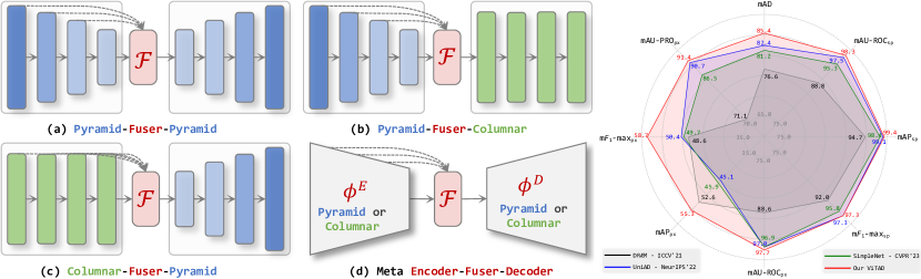
Figure 1: Left: (a-c) display general reconstruction-based AD frameworks. (d) shows abstracted Meta-AD framework that consists of image Encoder $\phi^{E}$, Fuser $\mathcal{F}$, and Decoder $\phi^{D}$. The dashed line indicates that the feature may be used by the Fuser $\mathcal{F}$. Right: Comprehensive quantitative comparison with popular methods by eight metrics on MVTec AD dataset [2] (Sec. 4.1 and Sec. 4.2).

Anomaly detection (AD) methods in the literature can mainly be broadly categorized as follows. 1) Augmentation-based methods [13, 3, 12] enhance performance by introducing fabricated anomaly information. 2) Embedding-based methods [14, 15, 16] map normal features to a compact space and identify anomalies by feature comparison. 3) Reconstruction-based methods usually follow an encoder-decoder framework to reconstruct inputs, which have gradually evolved from image-level to feature-level reconstructions for better segmentation accuracy. Simple reconstruction errors serve as the anomaly map during inference, and it only requires a pixel-level loss function without complex training constraints and tricks, which has better practicality. According to whether the encoder-decoder structure is pyramidal (i.e., ResNet [17]) or columnar (i.e., ViT [18]), existing methods can be categorized as fully pyramidal structures [19, 20, 11] (Fig. 1(a)), pyramidal encoder with a dynamic ViT [21, 12] (Fig. 1(b)), and columnar ViT-based encoder with a pyramidal decoder [22] (Fig. 1(c)). However, relying solely on none or a portion of global ViT modeling can lead to misdetections. We attribute the issues to the inadequacy of global semantic modeling capabilities, which motivates us to explore effective models to consider global interactions.

In contrast, the Meta-AD framework (Fig. 1(d)) consists of i) a feature Encoder to map the input to the latent space while compressing the spatial dimensions; ii) A feature Fuser to fuse multi-stage feature maps and generate more compact features as the decoder input; iii) A feature Decoder to reconstruct the original image or features to calculate the loss and anomaly map. Existing methods typically introduce pyramidal networks as encoders or decoders to obtain multi-resolution features for more accurate anomaly locations [1, 11, 12]. Nevertheless, columnar ViT serves as a visual foundation model that has been effective for possessing multi-scale modeling capabilities in other dense prediction tasks, e.g., object detection [23, 24], semantic segmentation [25, 26, 27, 28, 29], and human pose estimation [30, 31]. This motivates us to explore feasibility of using plain ViT for anomaly detection.

Within the Meta-AD framework, we propose a symmetrical plain ViT structure, instantiating a novel efficient ViTAD model that only includes global modeling, iinstead of the pyramidal encoder and decoder. Notably, we adopt a 12-layer ViT-S evenly divided into four stages to correspond to the standard ResNet-like structure [17]. We use the “multi-scale" rather than “multi-resolution" concept for describing features from multiple stages to avoid confusion. However, directly applying the original ImageNet-1k pre-trained ViT structure leads to poor anomaly classification and localization results. For instance, the image-level and pixel-level mAU-ROC metrics are only 93.6/96.2, significantly lower than the SoTA UniAD of 97.5/97.0. The substantial gap interests us in how the ViT structure adapts to anomaly detection. Adhering to Occam’s Razor principle, we refrain from developing new components in micro-structures or training tricks. Instead, we minimally adjust ViT from both macro and micro perspectives (Sec. 3.3) to explore its MUAD capability. From a macro perspective, we empirically identify three design factors that affect the model’s performance: 1) A columnar ViT with the same resolution shortens the information flow path, leading to potential information leakage. Removing skip connections of multi-scale features in Fuser can improve performance. 2) Due to the gap between industrial data and ImageNet [32], weights obtained from more generic and category-independent unsupervised training yield better results. 3) The last three stages can provide rich multi-scale information, and using them for loss constraints and anomaly map calculations enables the model to have higher anomaly localization capabilities. From a micro perspective, we further identify four minor structural details that slightly affect the model’s performance: 1) Whether the output for Encoder goes through the final batch normalization. 2) Whether the Fuser uses linear feature transformation. 3) Whether position embedding is used. 4) Whether the class token is inherited. Empirical experiments detail their effects. Additionally, we discovered several interesting findings: 1) Pyramidal structure for Encoder/Decoder is not necessary for AD models, and even plain ViT can yield impressive state-of-the-art (SoTA) results (Sec. 4.2 and Sec. 4.3). 2) The pre-training weights and model scale of the encoder significantly impact the results, and their performance in classification tasks does not consistently correlate with AD results (Sec. 4.5.2 and Sec. 4.5.3). 3) A heavy Fuser is not necessary that a superficial linear layer suffices, which contradicts the design conclusion of previous works [33, 11] (Sec. 4.5.1).

We replicate the results of recent mainstream methods [10, 11, 12, 34, 3] besides the open-source UniAD on MUAD, proposing a comprehensive and fair evaluation benchmark on eight metrics for the first time. Also, we explore various factors that may affect model performance in Sec. 4.5, and full code is available in supplementary materials. Surprisingly, extensive experiments on popular MVTec AD [2] and VisA [35] validate the effectiveness and efficiency of our approach. Even without elaborate structures and training tricks, our method achieves impressive results in Fig. 1-Right, e.g., reaching new SoTA image-level 98.3 mAU-ROC, 99.4 mAP, and 97.3 m$F_{1}$-max; pixel-level 97.7 mAU-ROC, 55.3 mAP, 58.7 m$F_{1}$-max, and 91.4 mAU-PRO; overall 85.4 mAD in the multi-class unsupervised setting, while requiring much less 1.1 hours and 2.3G of GPU memory to complete model training by one single V100 GPU.

In this work, we successfully apply columnar plain ViT to the MUAD task without any bells and whistles, achieving SoTA results and discussing some profound findings. This work can serve as a strong benchmark for the MUAD task both in terms of method comparison and evaluation manner, and inspire further research on ViT in the AD field. Our contributions are summarized as follows.

• At the task level, we replicate and benchmark different types of SoTA methods for fair comparisons under the increasingly researched MUAD task. We also propose using eight metrics to comprehensively evaluate different approaches for the first time (Sec. 4.1).

• From the methodological perspective, we first summarize existing reconstruction-based methods and abstract a Meta-AD concept (Sec. 3.2). Then, we instantiate a novel ViTAD model inspired by Meta-AD, which explores pure plain ViT as the fundamental structure for the first time. Specifically, ViTAD is effectively designed step by step from three macro and four micro perspectives (Sec. 3.3). Finally, we provide in-depth discussions and present some interesting findings.

• Extensive experimental evaluations with recent SoTA methods on popular MVTec AD and VisA datasets demonstrate the superior performance and efficiency of our ViTAD. We also explore and ablate factors that may affect model performance and robustness (Sec. 4.5). Finally, we reveal several potential future research based on the empirical results and findings.

2 Related Work

Visual Anomaly Detection is dedicated to classifying and segmenting abnormal images from normal ones, typically divided into supervised and unsupervised categories [1]. The former generally use synthetic data [36, 10, 37] or few-shot anomaly samples for semi-supervised model training [38, 39, 40, 41, 42, 43, 44], which can be seen as a particular case of a binary classification segmentation task. The general latter only requires normal training data to distinguish abnormal regions during testing, which can usually be divided into three taxonomies: 1) Augmentation-based methods [13, 10, 45, 46, 37, 12, 3] typically involve synthesizing abnormal regions on normal images or adding anomalous information to normal features to construct pseudo supervisory signals for better one-class classification. 2) Embedding-based methods map normal features to a compact space, distancing them from abnormal parts to ensure discriminative capabilities. Current approaches can be typically categorized into distribution-map-based [47, 48, 49, 50, 51, 52, 53, 54, 14, 55], teacher-student-based [56, 57, 34, 15, 58, 59], and memory-bank-based [60, 61, 62, 63, 64, 65, 16, 66]. 3) Reconstruction-based methods generally consist of an encoder and a decoder, with some approaches incorporating an additional transformation module. Anomaly localization is achieved by measuring the discrepancy between the input and reconstructed data, and current methods can be roughly categorized into two taxonomies based on the data being reconstructed, i.e., RGB image and deep features. Image-level methods [67, 68, 69, 70, 71, 72, 73, 74, 75] essentially follow the AutoEncoder (AE) idea that trains a network to reconstruct original normal RGB images [76, 77, 19, 78]. Works [79, 20, 80] introduces a deep generative adversarial network to learn normal manifold, while subsequent studies attempt to incorporate anomaly data augmentation strategies to enhance pseudo-supervision of the model, such as random noise generation [81], random mask generation [82], cut paste operation [83, 75], DRÆM-like predefined anomaly data construction schemes [10], etc.. Feature-level methods further extend to reconstructing more expressive deep features that generally achieve better performance [21, 84]. UniAD [12] corroborates the pivotal function of query embedding in circumventing shortcut feature-level distribution and further introduces a layer-wise query decoder to model feature-level distribution. Subsequent RD [11] introduces a novel “reverse distillation" paradigm to reconstruct multi-resolution features, which can be viewed as the extension over multi-resolution representations. Nevertheless, augmentation-/embedding-based methods achieve satisfactory results, but incorporating additional anomaly-related operations renders the model more complex, high-dimensional embeddings can be computationally expensive [61, 63], and noise-sensitive can lead to inaccurate anomaly detection [85]. Capitalizing on the simplicity and effectiveness of the reconstruction scheme, this paper investigates effective and efficient ViT-based designs for unsupervised AD for the first time.

Multi-class Unsupervised Anomaly Detection. Most existing methods require individual models for training each category [16, 10, 11, 75, 84, 3], a.k.a., Single-class Unsupervised Anomaly Detection (SUAD), which is superfluous, expensive, and time-consuming that is unsuitable for practical applications. Comparatively, UniAD [12] first employs one unified model to cover multiple categories, a.k.a., Multi-class Unsupervised Anomaly Detection (MUAD), recognized by follow-up works [86, 87, 88]. This paper also researches this more challenging but practical setting, pushing the results to a new level.

Pyramidal Architecture for Anomaly Detection. AD field has a consensus among researchers that multi-resolution (pyramidal) features are necessary to model accurate anomaly locations. Hence, early methods [89, 19, 75, 16, 11, 12, 84, 3] would introduce pyramidal networks in model design. However, they generally include a heavy backbone, and local modeling leads to a smaller receptive field that would cause misdetection of certain defects [16, 11, 3]. Only recently have some works introduced dynamic ViT [18] to model global information interaction to improve performance. However, they retain the pyramidal network in the Encoder [21, 12, 34] or Decoder [22, 90, 34]. Unlike these methods, this inspires us to explore solely using pure plain and columnar ViT for the MUAD task for the first time.

Plain Vision Transformer. Since Vision Transformer (ViT) [18] first introduced Transformer [91] structure into visual classification successfully, massive improvements have been subsequently developed [92, 93, 94, 95, 96, 97, 98]. Benefiting from global dynamic modeling capabilities, columnar plain ViT offers more excellent usability and practical values compared to the more complex pyramidal structures. Recently, researchers have been simplifying their approaches and attempting to employ plain ViT to tackle various downstream tasks, i.e., object detection [23], semantic segmentation [26, 99, 100, 101], in-context visual learning [27], human pose estimation [30, 31], etc.. Plain ViT has achieved impressive results above dense prediction tasks, demonstrating its strong multi-scale and pixel-level feature representation abilities. Comparatively, anomaly detection also potentially benefits from this capability, but columnar ViT is only partially used in current methods, e.g., in encoder [22] or decoder [21, 12]. This inspires us to break inherent bias, representing the first exploration of the potential and application value of plain ViT in the challenging MUAD task.

Besides, pre-trained weights of foundation ViT have a significant impact on downstream tasks. In addition to supervisorily-trained on ImageNet [32], many unsupervised pre-training methods [102, 103, 104, 105] may result in different feature distributions. This paper also explores the impact of different pre-training manners, finding that DINO-based weights yield the best results.

Efficient Network Design for Anomaly Detection. Model efficiency is important for practical applications, yet current methods are pursuing algorithmic accuracy while overlooking this aspect. For instance, DRÆM [10] has 97.4M parameters and requires 19.6 GPU hours under the condition of 300 epochs of training. UniAD [12] needs 1000 epochs to converge to satisfactory results, while RD [11] also requires a high parameter count of 80.6M due to its use of a pyramidal WideResNet-50 encoder/decoder. The excessive number of parameters and training time indicate that the model requires more storage and computational power, thus reducing its practical value. This paper adopts plain ViT-S [18] as the model architecture, which is more in line with mainstream technological development and more simple, elegant, and effective. Moreover, it only requires training for 100 epochs (only 1.1 GPU hours) to achieve clear advantages over SoTA methods.

3 Methodology: Abstract then Instantiate

3.1 Task Definition of MUAD

Similar to tasks such as classification [32] and object detection [106], a more practically valuable anomaly detection setting should involve a model handling multiple categories simultaneously. Given an AD dataset that contains $N$ classes $\bm{C}=\{\textit{C}_{1},\textit{C}_{2},\cdots,\textit{C}_{N}\}$, general Single-class Unsupervised AD (SUAD) setting only uses one class $\textit{C}_{i}$ ($i=1,2,\cdots,N$ indicates the class number) that contains one-class set $\chi_{i}=\{(\chi_{i,normal}^{Train}),(\chi_{i,normal}^{Test},\chi_{i,anomaly}^{Test})\}$ to train/test per experiment, i.e., $\bm{C}_{\textit{Train}}=\bm{C}_{\textit{Test}}=\textit{C}_{i}$; while more practical Multi-class Unsupervised AD (MUAD) setting covers all classes $\bm{C}$ that contain all-class sets $\chi=\sum_{i=1}^{N}\chi_{i}$ in one unified model, i.e., $\bm{C}_{\textit{Train}}=\bm{C}_{\textit{Test}}=\bm{C}$. As shown in Fig. 2, upper normal images of all classes marked in blue are used for training simultaneously without any extra labels information, i.e., no anomalous/defective images marked in red, while lower normal/abnormal samples are tested together to assess the binary classification capacity of the method. This challenging task is firstly described in UniAD [12] and is recognized by recent works [86, 87]. Specifically, we term sample-level detection and pixel-level location, which have been called in previous works by default, as classification and segmentation to avoid potential confusion.

3.2 Formulation of Meta-AD

This paper looks deeper at the reconstruction-based method for multi-class unsupervised anomaly detection. As mentioned above in Fig. 3-(d), we abstract current reconstruction-based approaches roughly by a meta framework that contains a feature Encoder, a Fuser, and a Decoder. Fig. 3 details the specific process of its structural treatment and symbols.
1) Feature Encoder maps the input stem feature map $F_{0}$ to multi-scale deep features. In the macro architecture, $\phi^{E}$ consists of multiple stages $\{{\color[rgb]{0.69140625,0.140625,0.09375}\bm{\phi^{E}_{1}}},{\color[rgb]{0.69140625,0.140625,0.09375}\bm{\phi^{E}_{2}}},$…$,{\color[rgb]{0.69140625,0.140625,0.09375}\bm{\phi^{E}_{N}}}\}$ with each containing many basic blocks. And it can be either a pyramidal structure with a decreasing resolution (e.g., ResNet [17] and EfficientNet [107]) or a columnar structure with a consistent resolution (e.g., ViT [18]); In the micro component, it can be either CNN-based [11] or Transformer-based [108]. Pyramidal structures [11, 12, 108] are more commonly used for the strong ability to extract rich multi-scale features $F=\{F_{0},F_{1},\dots,F_{N}\}$. Denote $i$-th feature extract by the encoder ${\color[rgb]{0.69140625,0.140625,0.09375}\bm{\phi^{E}_{i}}}$ as $F_{i}\in\mathcal{R}^{C_{i}\times H_{i}\times W_{i}}$, where $C_{i}$, $H_{i}$, and $W_{i}$ represent channel, height, and weight, respectively. The encoding process can be represented as:

$$F_{i}={\color[rgb]{0.69140625,0.140625,0.09375}\bm{\phi^{E}_{i}}}(F_{i-1}),~{}~{}~{}i=(1,2,\dots,N),$$ (1)

where the resolution of $\phi^{E}_{i}$ equals $\phi^{E}_{i-1}$ if columnar encoder is employed, and vice versa.

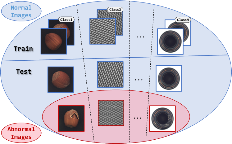
Figure 2: Diagram of Multi-class Unsupervised AD setting.

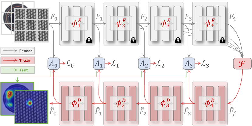
Figure 3: Intuitive visualization of reconstruction-based Meta-AD paradigm, which consists of a pre-trained image encoder $\phi^{E}$ to obtain features at different depths from the patch embedding input, a feature fuser $\mathcal{F}$ to aggregate extracted multiple features, and a decoder $\phi^{D}$ that has the same structure with the encoder to reconstruct multi-depth features. During the training phase, $\hat{F}_{i}$ is constrained by $F_{i}$ with loss function $\mathcal{L}_{i}$ to update $\phi^{D}$, while both $\hat{F}_{i}$ and $F_{i}$ are used to calculate anomaly map $A_{i}$ for inference.

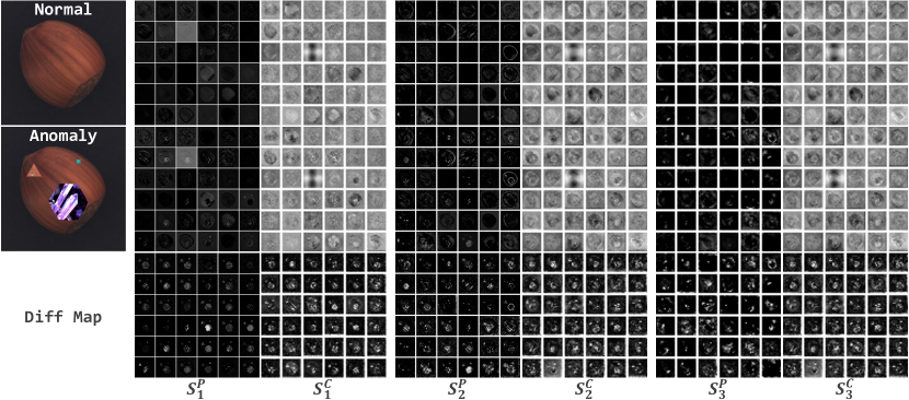
Figure 4: The first 36 visualized feature maps of different stages ($S_{i}$, $i=1,2,3$) for pyramid [11] ($S^{P}$) and columnar [18] ($S^{C}$) backbones. First two rows show results of normal and anomaly images in the first column, and the last row shows differential maps. Results demonstrate the superiority of ViT for capturing more abundant features and locating more distinct anomalous regions.

2) Feature Fuser bridges the encoder and decoder that could fuse multi-layer features $\{F_{0},F_{1},\dots,F_{N}\}$ from different stages and produce a more compact feature for the decoder. Generally, there are two main ideas to design this module: a) the light structure to fuse multi-scale features efficiently [12]; and b) the heavy structure to obtain better representation [11]. Without loss of generality, the Fuser $\mathcal{F}$ takes multi-layer features as the input to obtain the fused feature $\hat{F}_{f}$, denoted as:

$$\hat{F}_{f}={\color[rgb]{0.69140625,0.140625,0.09375}\bm{\mathcal{F}}}(\theta_{0}(F_{0}),\theta_{1}(F_{1}),\dots,\theta_{N}(F_{N})),$$ (2)

where $\theta_{i}$ is used to adjusts $i$-th feature to the desired size for subsequent fusion processing, e.g., up-sampling and de-convolution operations. Specifically, $\theta_{i}$ does not change the resolution of the $i$-th feature in the case of the columnar encoder. The model degenerates into an Auto Encoder structure when only the last compressed feature $F_{N}$ is used, i.e., $\hat{F}_{f}$ equals $\hat{F}_{N}$.

3) Feature Decoder reconstructs original images or encoded features from the fused feature $\hat{F}_{f}$. Similar to the encoder, decoder $\phi^{D}$ can be a pyramidal/columnar structures. Pyramid CNN is the most commonly used structure because the fused feature usually needs to be up-sampled to match the resolution of encoded features for accurate anomaly localization. The reconstruction process can be formulated as follows:

$$\hat{F}_{i-1}={\color[rgb]{0.69140625,0.140625,0.09375}\bm{\phi^{D}_{i}}}(\hat{F}_{i}),~{}~{}~{}i=(1,2,\dots,N),$$ (3)

where the resolution of $\phi^{E}_{i}$ equals $\phi^{E}_{i-1}$ if columnar encoder is employed, and vice versa.

4) Anomaly Map Estimation. Reconstruction-based AD methods employ reconstruction error to describe anomaly regions, which assumes that anomalies cannot be well reconstructed due to their absence during the training process. For the $i$-th stage, the anomaly map $A_{i}$ is calculated by:

$$A_{i}=\mathcal{L}_{i}(F_{i},\hat{F}_{i}),~{}~{}~{}i=(1,2,\dots,N),$$ (4)

where $\mathcal{L}_{i}$ can be L1, Mean Square Error (MSE), Cosine Distance, etc. During the training phase, $A=\Sigma_{i}^{N}A_{i}$ is used as the only loss to backward the gradient, while $A=\Sigma_{i}^{N}{A_{i}}$ serves as the anomaly map for testing. Nevertheless, some construction-based works employ extra losses [84, 75] to boost performance, but they suffer from hard modeling and inelegant implementation, and we argue that using only one simplest pixel-level loss is sufficient for Meta-AD.

5) Generalized Extension. In the generalized concept, encoder features can skip directly to multiple decoder stages without going through the Fuser [80]. Still, this manner is prone to fall into an “identity shortcut" that appears to return an unmodified input disregarding its input content [12], resulting in unsatisfactory expectations. Nevertheless, this paper does not discuss this manner, but the abstracted Meta-AD framework can be easily extended to include that case.

3.3 Plain Vision Transformer for AD

3.3.1 Motivation for exploring plain ViT for the MUAD task

Thanks to the global dynamic modeling capabilities, plain ViT possesses strong multi-scale representation abilities and robustness, which have been proven effective in multiple domains, i.e., object detection [23], semantic segmentation [26], in-context visual learning [27], multi-modal fusion [109], etc. However, relying solely on none or a portion of global ViT modeling can lead to misdetection of certain types of defects [22, 21, 12], e.g., logical errors and long-distance interactions (i.e., “cable swap" and “combined" in cable category on MVTec AD [2]) as follows:

Therefore, this paper explores the possibility of purely using plain ViT for MUAD, and as analyzed in Sec. 1, anomaly detection can also potentially benefit from these attributes of ViT: 1) For the modeling manner, attention-based ViT employs the dynamic modeling mechanism to extract input-adapted features, which allows for stronger modeling capability and generalization compared to the static CNNs [92, 23, 26]. As shown in Fig. 4, ViT-oriented features are richer and more diversified than CNN’s at each stage, and the difference between normal and abnormal images becomes more pronounced, which is beneficial for anomaly localization. 2) For the receptive field, global-modeling ViT, as opposed to the local-modeling CNNs, provides a larger receptive field, enabling it to capture potential long-range correlations among distant positions better. Furthermore, from the frequency domain perspective, ViT is capable of modeling both high-/low-frequency information simultaneously, while CNN is more adept at high-frequency information modeling. This endows ViT with the ability to locate subtle defects, an ability that is particularly important for precise anomaly detection tasks [110]. 3) For the practicability, as the modern foundational model, ViT can be effortlessly adapted for multi-modal inputs, which is endowed with versatility and potential in handling diverse AD applications in future works, i.e., multi-modal 3D AD [111, 112], zero-shot AD [40, 41, 113]. However, plain ViT has never been explored in AD because there seems to be a consensus among researchers that multi-resolution features are necessary to model accurate anomaly location, so most current AD methods would introduce a pyramidal network in Encoder [21, 12, 34] or Decoder [22, 34] to obtain multi-resolution features. This inspires us to explore whether only a plain, simple, and columnar ViT is up to the MUAD task.

Starting from Meta-AD, we employ columnar plain ViT as the instantiated structure and divide it into four stages for both Encoder $\{{\color[rgb]{0.69140625,0.140625,0.09375}\bm{\phi^{E}_{1}}},{\color[rgb]{0.69140625,0.140625,0.09375}\bm{\phi^{E}_{2}}},{\color[rgb]{0.69140625,0.140625,0.09375}\bm{\phi^{E}_{3}}},{\color[rgb]{0.69140625,0.140625,0.09375}\bm{\phi^{E}_{4}}}\}$ and Decoder $\{{\color[rgb]{0.69140625,0.140625,0.09375}\bm{\phi^{D}_{1}}},{\color[rgb]{0.69140625,0.140625,0.09375}\bm{\phi^{D}_{2}}},{\color[rgb]{0.69140625,0.140625,0.09375}\bm{\phi^{D}_{3}}},{\color[rgb]{0.69140625,0.140625,0.09375}\bm{\phi^{D}_{4}}}\}$, respectively, with each stage containing the same number of layers, i.e., 3 for each stage with 12-layer ViT-B trained on ImageNet-1K as the backbone by default, and the Decoder is randomly initialized with the ViT structure. For the feature Fuser F, we employ one superficial linear layer to aggregate concatenated multi-stage features with the same resolution to ensure that the channel number of $\hat{F}_{f}$ matches the decoder input, denoted as:

$$\hat{F}_{f} ={\color[rgb]{0.69140625,0.140625,0.09375}\bm{\mathcal{F}}}(F_{1},\dots,F_{4})$$ (5)

$$=\text{Linear}([F_{1},\dots,F_{4}]),$$

where $\theta_{i}$ in Eq. 5 degenerates into identity operation for simplicity. Nevertheless, naive implementation yields a significant gap compared to the SoTA methods on the MUAD task, e.g., the image-level and pixel-level mAU-ROC metrics are only 93.6/96.2, which is significantly lower than the SoTA UniAD of 97.5/97.0. Thus, we further make AD-specific improvements to the implementation details at both macro and micro levels in Fig. 5, ultimately achieving obvious superiority over SoTA pyramidal approaches (Sec. 4.2 and Sec. 4.3). This indicates that pyramidal structure for Encoder/Decoder is not necessary for AD models, and even plain ViT can yield impressive SoTA results (Finding 1).

3.3.2 Macro-level Design of ViTAD

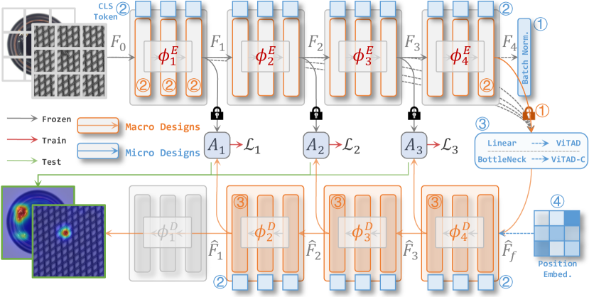
Figure 5: Detailed structure of instantiated ViTAD from Meta-AD. Partial structures represented by the orange and blue numbers respectively indicate the adaptations of the plain ViT at the macro and micro levels for anomaly detection.

TABLE I: Empirical study on different pre-trained weights of ViT-S. IN1K: pretrained on ImageNet-1K. IN22K: first pre-trained on ImageNet-22K, then fine-tuned on ImageNet-1K. ^∗: with patch size equaling 8. ^†: with further 384 resolution. Note that ViT-B is used for MAE and CLIP due to the absence of the ViT-S model.

Model	Image-level				Pixel-level					mAD
	mAU-ROC	mAP	m$F_{1}$-max		mAU-ROC	mAP	m$F_{1}$-max	mAU-PRO
Rand	59.5	79.5	84.7		74.7	15.3	20.4	45.7		54.2
IN1K	94.4	97.5	95.3		96.6	51.6	54.5	87.2		82.4
IN22K	95.6	97.7	95.5		97.1	51.6	55.3	87.7		82.9
DeiT	95.8	98.1	96.1		97.1	53.9	56.8	87.8		83.7
CLIP	71.2	84.5	85.7		81.6	19.4	25.1	56.8		60.6
MoCo	95.3	97.7	95.2		97.4	53.0	56.2	90.6		83.6
MAE	95.3	97.7	95.2		97.4	53.0	56.2	90.6		83.6
DINO	98.3	99.4	97.3		97.7	55.3	58.7	91.4		85.4
DINO∗	97.0	98.8	96.6		98.2	63.2	63.6	93.2		87.2
DINO†	97.3	98.9	96.3		98.3	66.7	65.7	93.4		88.1

TABLE II: Empirical study on restraint stages. Numbers represent the constrained stages.

Restraint Stage	Image-level				Pixel-level					mAD
	mAU-ROC	mAP	m$F_{1}$-max		mAU-ROC	mAP	m$F_{1}$-max	mAU-PRO
3	95.2	98.0	94.6		96.9	50.0	54.7	87.1		82.4
2,3	97.0	98.8	96.3		97.4	52.3	57.1	89.2		84.0
1,2,3	98.3	99.4	97.3		97.7	55.3	58.7	91.4		85.4
0,1,2,3	95.5	97.6	95.2		97.4	53.5	57.4	90.5		83.9

As shown by the orange numbers in Fig. 5, we have explored three effective design improvements at the macro level for the ViT-based AD model: 1) Fuser removes the multi-scale feature skip connection and only uses the last stage $F_{4}$ as input, i.e., $\hat{F}_{f}=\text{Linear}(F_{4})$ for Eq. 5. This significantly improves the image-level performance. The mAU-ROC/mAP/mAP/m$F_{1}$-max metrics respectively increase by +0.7/+0.4/+0.9, while the pixel-level results remain almost unchanged (Tab. VIII). The reason is that the deep features $F_{4}$ of the columnar ViT are sufficient to contain rich texture and semantic attributes. The injection of early features would shorten the information flow path, leading to potential information leakage and affecting the model’s judgment ability at the image level. Furthermore, we experientially observe that a heavy Fuser is not necessary and a simple linear layer suffices, which contradicts the design conclusion of previous works [33, 11] (Sec. 4.5.1). 2) Current AD methods usually use pre-trained weights on ImageNet-1K [32] as part of the model. However, the direct application may not obtain good results due to the gap between ImageNet-1K and industrial data. We study the pros and cons of self-supervised training manners, finding that weights obtained from more general and class-independent unsupervised training yield better results. As shown in Sec. 4.5.2, larger supervised models and pre-training manners improve results (IN22K vs. IN1K). DINO [103] has a stronger semantic granularity and achieves significantly better results than other pre-training methods. It’s worth mentioning that MAE [105] does not achieve the expected results, reasoning that the pre-training paradigm with a shallow decoder leads to weaker feature semantic expression (Finding 2). Furthermore, we find that a smaller patch size (i.e., 8) and higher resolution significantly improve pixel-level indicators and overall mAD. Although a slight decrease in image-level indicators accompanies this, improving segmentation results provides more valuable guidance for practical applications. 3) Features at different levels have various granularities of expression. By default, this paper uses $F_{1}$/$F_{2}$/$F_{3}$ for training constraints and the calculation of anomaly maps $A_{1}$/$A_{2}$/$A_{3}$ during inference. This configuration provides rich multi-scale information to produce more accurate anomaly localization. As shown in Tab. II, using fewer/more feature combinations decreases performance significantly.

3.3.3 Micro-level Modification of ViTAD

TABLE III: Empirical study on structural details. Before Norm: $F_{4}$ is obtained before normalization. Add Linear: Add the linear layer in Fuser. Use Pos. Embed.: Keeping the position embedding in the decoder. Remove CLS Token: Removing the class token throughout the procedure.

Before Norm	Add Linear	Use Pos. Embed.	Remove CLS Token	Image-level	Pixel-level	mAD
✘	✘	✘	✘	97.6/99.0/96.8	97.5/55.0/58.2/91.0	85.0
✔	✘	✘	✘	97.9/99.1/97.0	97.5/54.8/58.1/91.1	85.1
✘	✔	✘	✘	97.8/99.1/96.8	97.6/55.1/58.3/91.2	85.1
✘	✘	✔	✘	97.6/99.1/96.8	97.6/55.2/58.2/91.2	85.1
✘	✘	✘	✔	97.7/99.1/96.8	97.6/55.0/58.3/91.2	85.1
✘	✔	✔	✔	98.1/99.2/97.0	97.7/55.2/58.5/91.0	85.2
✔	✘	✔	✔	98.1/99.2/97.0	97.6/55.0/58.3/91.1	85.2
✔	✔	✘	✔	98.0/99.1/97.2	97.7/55.3/58.5/91.3	85.3
✔	✔	✔	✘	98.0/99.1/97.2	97.6/55.1/58.3/91.3	85.2
✔	✔	✔	✔	98.3/99.4/97.3	97.7/55.3/58.7/91.4	85.4

Furthermore, as indicated by the blue numbers in Fig. 5, we attempt four effective detailed designs at the micro level, investigating some structural details that potentially impact performance. Specific quantitative results are displayed in Tab. III. 1) Using features before normalization rather than after as the fusion features slightly decreases image-level performance. 2) By default, we use a lightweight one linear layer as the Fuser structure that discards heavy transformations. Going a step further, we remove this linear layer, i.e., $F_{4}$=$\hat{F}_{4}$, and find that the overall metrics show a slight decline, indicating the necessity of one linear layer (Finding 3). 3) Keeping the position embedding of the ViT-based Decoder also brings a slight performance increase. 4) Keeping the class token throughout the process would slightly decline overall metrics, implying that the class token might interfere with the semantics at the normal spatial structure level that leads to a decrease in abnormal classification ability.

3.3.4 Training Constraints

ViTAD aims at using the fused feature $\hat{F}_{f}$ to reconstruct multiple features $F_{i}\in\mathcal{R}^{C_{i}\times H_{i}\times W_{i}}$ by the predicted $\hat{F}_{i}\in\mathcal{R}^{C_{i}\times H_{i}\times W_{i}}$ with decoder. Let $F_{i}(h,w)\in\mathcal{R}^{C_{i}}$ and $\hat{F}_{i}(h,w)\in\mathcal{R}^{C_{i}}$ be the $i$-th stage feature vector at position $(h,w)$ in both encoder and decoder, we use the cosine distance at position $(h,w)$ as the anomaly score $A_{i}(h,w)$:

$$A_{i}(h,w)=1-\frac{F_{i}(h,w)^{T}\cdot\hat{F}_{i}(h,w)}{\|F_{i}(h,w)\|\|\hat{F}_{i}(h,w)\|},i\in\{1,2,3\}.$$ (6)

Anomaly scores of all positions construct the final anomaly map. Since the model is only trained on normal samples, the large pixel values in the anomaly map suggest anomalies. For the $i$-th stage, the corresponding loss term $\mathcal{L}_{i}$ is calculated by:

$$\mathcal{L}_{i}=\frac{1}{H_{i}W_{i}}\sum_{h=1}^{H_{i}}\sum_{w=1}^{W_{i}}A_{i}(h,w).$$ (7)

The overall loss $\mathcal{L}_{All}=\Sigma_{1}^{3}{\mathcal{L}_{i}}$ is the simple sum of all $\mathcal{L}_{i}$ terms.

3.3.5 Anomaly Segmentation and Classification

Anomaly segmentation aims to provide the pixel-level anomaly score map to determine the specific locations of the anomalies. Multi-scale anomaly maps $\{A_{1},A_{2},A_{3}\}$ calculated by the restrained features are summed up to form the final anomaly map $A$=$\text{sum}(A_{1},A_{2},A_{3})$ for evaluation. Besides, anomaly classification requires an image-level anomaly score to indicate whether the image is anomalous. Following work [12], we first apply an average pooling operation to the anomaly score map $A$ and then take its maximum value as the anomaly score.

4 Experiments and Discussions

4.1 Setup for Multi-class Unsupervised AD

Datasets. We evaluate ViTAD as well as comparison methods on popular MVTec AD [2, 114] and VisA [35] datasets for both anomaly classification and segmentation: The former dataset contains 15 industrial products in 2 types with 3,629 normal images for training and 467/1,258 normal/anomaly images for testing (5,354 images in total); The latter covers 12 objects in 3 types with 8,659 normal images for training and 962/1,200 normal/anomaly images for testing (10,821 images in total). Both two datasets provide ground-truth anomaly maps at the pixel level for evaluation.

Task Setting. Traditionally, the single-class setting requires training a cumbersome model for each class separately, and the metric results have almost reached saturation. Therefore, we focus on the more challenging and practical multi-class setting in this work. Experiments for ablation and interpretability are primarily conducted on the MVTec AD dataset.

Re-regulation of Comprehensive Metric for AD. Following prior works [11, 10, 35, 15], we use threshold-independent sorting metrics: 1) mean Area Under the Receiver Operating Curve (mAU-ROC) to evaluate binary classification ability; 2) mean Average Precision [10] (mAP) to calculate the area under the PR curve; 3) mean Area Under the Per-Region-Overlap [15] (mAU-PRO) to weight regions of different size equally. Also, threshold-dependent 4) mean $F_{1}$-score at optimal threshold [35] (m$F_{1}$-max) is further employed to relieve potential data imbalance problem of implausible evaluation. Note that mAU-ROC, mAP, and m$F_{1}$-max are used in both image-level (anomaly classification) and pixel-level (anomaly segmentation) evaluations. For all methods, the models are by default tested ten times evenly, and the epoch result corresponding to the maximum pixel-level mAU-ROC value is taken as the final result. We strongly recommend using the above seven metrics to evaluate various methods more fully, and the mean metric of all the metrics (termed mAD) is further reported to indicate the overall capability of a model, as each metric has specific flaws.

TABLE IV: Comparison for concurrent powerful methods. ✔: Satisfied; ✘: Unsatisfied; ✚: Partially satisfied; $\bigcirc$: Inapplicable.

Criterion $\rightarrow$	Pyramidal Encoder	Heavy Fuser	Pyramidal Decoder	Multi-Resolution Features	Image/Feature Augmentation	Category			00000000Reproduction 00000000Code
Method $\downarrow$						Aug.	Emb.	Rec.
DRÆM [10]	✔	✘	$\bigcirc$	✔	✔	✔	✚	✚	github.com/VitjanZ/DRAEM
RD [11]	✔	✔	✔	✔	✘	✘	✘	✔	github.com/hq-deng/RD4AD
UniAD [12]	✔	✘	✘	✔	✔	✔	✘	✔	github.com/zhiyuanyou/UniAD
DeSTSeg [34]	✔	✘	$\bigcirc$	✔	✔	✔	✔	✘	github.com/apple/ml-destseg
SimpleNet [3]	✔	✘	$\bigcirc$	✔	✔	✔	✔	✘	github.com/DonaldRR/SimpleNet
ViTAD (Ours)	✘	✘	✘	✘	✘	✘	✘	✔	github.com/zhangzjn/ADer

TABLE V: Image-level multi-class anomaly classification results with mAU-ROC/mAP/m$F_{1}$-max metrics on MVTec AD. Note that only one model is trained to detect anomalies for all categories. Superscript ^∗: Re-trained under the multi-class setting by the official code. ^†: Reproduced results no less than the original paper. Bold and Underline indicate optimal and sub-optimal results, respectively. The circled number represents the category to which the method belongs (c.f., Sec. 2): ➀-Image/Feature augmentation based; ➁-Embedding based; ➂-Image/Feature Reconstruction based, and the red circle indicate the main category to which the method belongs. Subsequent tables follow the consistent presentations.

Method $\rightarrow$		➀ ➁ ➂	➂	➀ ➂	➀ ➁	➀ ➁	➂
		DRÆM∗ [10]	RD∗ [11]	UniAD† [12]	DeSTSeg∗ [34]	SimpleNet∗ [3]	ViTAD
Category $\downarrow$		ICCV’21	CVPR’22	NeurIPS’22	CVPR’23	CVPR’23	(Ours)
Texture	Carpet	97.2/99.1/96.7	98.5/99.6/97.2	99.8/99.9/99.4	97.6/99.3/96.6	95.9/98.8/94.9	99.5$\pm.00$/99.9$\pm.00$/99.4$\pm.00$
	Grid	99.2/99.7/98.2	98.0/99.4/96.6	99.3/99.8/99.1	97.9/99.2/96.6	97.6/99.2/96.4	99.7$\pm.14$/99.9$\pm.05$/99.1$\pm.50$
	Leather	97.7/99.3/95.0	100./100./100.	100./100./100.	99.2/99.8/98.9	100./100./100.	100.$\pm.00$/100.$\pm.00$/100.$\pm.00$
	Tile	100./100./100.	98.3/99.3/96.4	99.9/99.9/99.4	97.0/98.9/95.3	99.3/99.8/98.8	100.$\pm.00$/100.$\pm.00$/100.$\pm.00$
	Wood	100./100./100.	99.2/99.8/98.3	98.9/99.7/97.5	99.9/100./99.2	98.4/99.5/96.7	98.7$\pm.10$/99.6$\pm.03$/96.7$\pm.47$
Object	Bottle	97.3/99.2/96.1	99.6/99.9/98.4	100./100./100.	98.7/99.6/96.8	100./100./100.	100.$\pm.00$/100.$\pm.00$/100.$\pm.00$
	Cable	61.1/74.0/76.3	84.1/89.5/82.5	94.8/97.0/90.7	89.5/94.6/85.9	97.5/98.5/94.7	98.5$\pm.15$/99.1$\pm.08$/95.7$\pm.86$
	Capsule	70.9/92.5/90.5	94.1/96.9/96.9	93.7/98.4/96.3	82.8/95.9/92.6	90.7/97.9/93.5	95.4$\pm.46$/99.0$\pm.12$/95.5$\pm.05$
	Hazelnut	94.7/97.5/92.3	60.8/69.8/86.4	100./100./100.	98.8/99.2/98.6	99.9/100./99.3	99.8$\pm.13$/99.9$\pm.07$/98.6$\pm.82$
	Metal Nut	81.8/95.0/92.0	100./100./99.5	98.3/99.5/98.4	92.9/98.4/92.2	96.9/99.3/96.1	99.7$\pm.07$/99.9$\pm.02$/98.4$\pm.30$
	Pill	76.2/94.9/92.5	97.5/99.6/96.8	94.4/99.0/95.4	77.1/94.4/91.7	88.2/97.7/92.5	96.2$\pm.50$/99.3$\pm.10$/96.4$\pm.18$
	Screw	87.7/95.7/89.9	97.7/99.3/95.8	95.3/98.5/92.9	69.9/88.4/85.4	76.7/90.5/87.7	91.3$\pm.39$/97.0$\pm.16$/93.0$\pm.88$
	Toothbrush	90.8/96.8/90.0	97.2/99.0/94.7	89.7/95.3/95.2	71.7/89.3/84.5	89.7/95.7/92.3	98.9$\pm.32$/99.6$\pm.12$/96.8$\pm.92$
	Transistor	77.2/77.4/71.1	94.2/95.2/90.0	99.8/99.8/97.5	78.2/79.5/68.8	99.2/98.7/97.6	98.8$\pm.57$/98.3$\pm.85$/92.5$\pm.72$
	Zipper	99.9/100./99.2	99.5/99.9/99.2	98.6/99.6/97.1	88.4/96.3/93.1	99.0/99.7/98.3	97.6$\pm.08$/99.3$\pm.03$/97.1$\pm.46$
Average		88.8/94.7/92.0	94.6/96.5/95.2	97.5/99.1/97.3	89.2/95.5/91.6	95.3/98.4/95.8	98.3$\pm.02$/99.4$\pm.05$/97.3$\pm.20$

Discuss with Comparison Methods. Considering that MUAD is a relatively recent task, this paper primarily compares with the publicly published UniAD [12], which first proposes this more practical setting. Simultaneously, we compare with the latest Augmentation-based DRÆM [10], Reconstruction-based RD [11], as well as Embedding-based DeSTSeg [34]/SimpleNet [3]. The official codes extend these methods to fair training for the unified MUAD setting. Also, we replace the ViT [18] encoder of our ViTAD with various pre-trained manners to ensure fair and comprehensive comparisons, including supervisorily pre-trained models by ImageNet [32] and self-supervised MOCO [102], MAE [105], CLIP [104], and DINO [103]. To clearly show differences among concurrent approaches, we suggest five criteria to compare current approaches clearly. As shown in Tab. IV, comparison methods more or less require 1) pyramidal encoder, 2) heavy fuser to aggregate multi-depth features, 3) pyramidal decoder, 4) multi-resolution features to keep accurate anomaly location ability, and 5) feature augmentation to obtain better results. On the contrary, our ViTAD seeks simplicity but effectiveness in design that does not require elaborate structure or complex augmentations.

Training Details. ViTAD is trained under 256 $\times$ 256 resolution without any extra datasets and training tricks/augmentations for all experiments by default. AdamW optimizer [115] is used with an initial learning rate of 1e^-4, a weight decay of 1e^-4, and a batch size of 8. Our model is trained for 100 epochs on a single GPU in all experiments, and the learning rate drops by 0.1 after 80 epochs, which is significantly lower compared with counterparts, e.g.,

DRÆM [10]	RD [11]	UniAD [12]	SimpleNet [3]	ViTAD
700	200	1,000	100	100

All categories are trained together without any categorical labels accessible in multiple cases, and we also report single-class results to evaluate our ViT-based approach fully. Note that the above hyper-parameters remain the same in all experiments under different settings and datasets for our approach without elaborate fine-tuning.

4.2 Quantitative Comparisons with SoTAs on MVTec AD

TABLE VI: Pixel-level multi-class anomaly segmentation with mAU-ROC/mAP/m$F_{1}$-max/mAU-PRO on MVTec AD. The last row presents the averaged mAD metric across seven metrics to provide a comprehensive evaluation.

Method $\rightarrow$		DRÆM∗ [10]	RD∗ [11]	UniAD† [12]	DeSTSeg∗ [34]	SimpleNet∗ [3]	ViTAD
Category $\downarrow$		ICCV’21	CVPR’22	NeurIPS’22	CVPR’23	CVPR’23	(Ours)
Texture	Carpet	98.1/78.7/73.1/93.1	99.0/58.5/60.5/95.1	98.4/51.4/51.5/94.4	93.6/59.9/58.9/89.3	97.4/38.7/43.2/90.6	99.0$\pm.01$/60.5$\pm.60$/64.1$\pm.22$/94.7$\pm.19$
	Grid	99.0/44.5/46.2/92.1	99.2/46.0/47.4/97.0	97.7/23.7/30.4/92.9	97.0/42.1/46.9/86.8	96.8/20.5/27.6/88.6	98.6$\pm.01$/31.2$\pm.16$/36.7$\pm.12$/95.8$\pm.82$
	Leather	98.9/60.3/57.4/88.5	99.3/38.0/45.1/97.4	98.8/34.2/35.5/96.8	99.5/71.5/66.5/91.1	98.7/28.5/32.9/92.7	99.6$\pm.01$/52.1$\pm.76$/55.8$\pm.66$/97.9$\pm.30$
	Tile	99.2/93.6/86.0/97.0	95.3/48.5/60.5/85.8	92.3/41.5/50.3/78.4	93.0/71.0/66.2/87.1	95.7/60.5/59.9/90.6	96.6$\pm.01$/56.4$\pm.26$/68.8$\pm.14$/87.0$\pm.44$
	Wood	96.9/81.4/74.6/94.2	95.3/47.8/51.0/90.0	93.2/37.4/42.8/86.7	95.9/77.3/71.3/83.4	91.4/34.8/39.7/76.3	96.4$\pm.03$/60.6$\pm.52$/58.3$\pm.39$/88.0$\pm.69$
Object	Bottle	91.3/62.5/56.9/80.7	97.8/68.2/67.6/94.0	98.0/67.0/67.9/93.1	93.3/61.7/56.0/67.5	97.2/53.8/62.4/89.0	98.8$\pm.03$/79.9$\pm.57$/75.6$\pm.56$/94.3$\pm.12$
	Cable	75.9/14.7/17.8/40.1	85.1/26.3/33.6/75.1	96.9/45.4/50.4/86.1	89.3/37.5/40.5/49.4	96.7/42.4/51.2/85.4	96.2$\pm.25$/43.1$\pm.54$/47.4$\pm.65$/90.2$\pm.74$
	Capsule	50.5/06.0/10.0/27.3	98.8/43.4/50.1/94.8	98.8/45.6/47.7/92.1	95.8/47.9/48.9/62.1	98.5/35.4/44.3/84.5	98.3$\pm.02$/42.7$\pm.58$/47.8$\pm.28$/92.0$\pm.94$
	Hazelnut	96.5/70.0/60.5/78.7	97.9/36.2/51.6/92.7	98.0/53.8/56.3/94.1	98.2/65.8/61.6/84.5	98.4/44.6/51.4/87.4	99.0$\pm.01$/64.6$\pm.46$/64.0$\pm.25$/95.2$\pm.08$
	Metal Nut	74.4/31.1/21.0/66.4	93.8/62.3/65.4/91.9	93.3/50.9/63.6/81.8	84.2/42.0/22.8/53.0	98.0/83.1/79.4/85.2	96.4$\pm.14$/75.1$\pm.52$/77.3$\pm.83$/92.4$\pm.13$
	Pill	93.9/59.2/44.1/53.9	97.5/63.4/65.2/95.8	96.1/44.5/52.4/95.3	96.2/61.7/41.8/27.9	96.5/72.4/67.7/81.9	98.7$\pm.01$/77.8$\pm.27$/75.2$\pm.23$/95.3$\pm.15$
	Screw	90.0/33.8/40.7/55.2	99.4/40.2/44.7/96.8	99.2/37.4/42.3/95.2	93.8/19.9/25.3/47.3	96.5/15.9/23.2/84.0	99.0$\pm.03$/34.0$\pm.81$/41.0$\pm.95$/93.5$\pm.53$
	Toothbrush	97.3/55.2/55.8/68.9	99.0/53.6/58.8/92.0	98.4/37.8/49.1/87.9	96.2/52.9/58.8/30.9	98.4/46.9/52.5/87.4	99.1$\pm.04$/51.3$\pm.95$/61.9$\pm.50$/90.9$\pm.17$
	Transistor	68.0/23.6/15.1/39.0	85.9/42.3/45.2/74.7	97.4/61.2/63.0/93.5	73.6/38.4/39.2/43.9	95.8/58.2/56.0/83.2	93.9$\pm.13$/58.4$\pm.36$/55.3$\pm.42$/76.8$\pm.88$
	Zipper	98.6/74.3/69.3/91.9	98.5/53.9/60.3/94.1	98.0/45.0/51.9/92.6	97.3/64.7/59.2/66.9	97.9/53.4/54.6/90.7	95.9$\pm.07$/42.6$\pm.43$/50.8$\pm.30$/87.2$\pm.82$
Average		88.6/52.6/48.6/71.1	96.1/48.6/53.8/91.2	97.0/45.1/50.4/90.7	93.1/54.3/50.9/64.8	96.9/45.9/49.7/86.5	97.7$\pm.02$/55.3$\pm.11$/58.7$\pm.10$/91.4$\pm.21$
mAD		76.6	82.3	82.4	77.1	81.2	85.4

TABLE VII: Multi-class image-level anomaly classification and pixel-level anomaly segmentation results on VisA.

		Image-level mAU-ROC/mAP/m$F_{1}$-max					Pixel-level mAU-ROC/mAP/m$F_{1}$-max/mAU-PRO
Method $\rightarrow$		DRÆM∗ [10]	UniAD† [12]	SimpleNet∗ [3]	ViTAD		DRÆM∗ [10]	UniAD† [12]	SimpleNet∗ [3]	ViTAD
Category $\downarrow$		➀ ICCV’21	➂ NeurIPS’22	➁ CVPR’23	➂ (Ours)		➀ ICCV’21	➂ NeurIPS’22	➁ CVPR’23	➂ (Ours)
Complex Structure	PCB1	71.9/72.3/70.0	94.2/92.9/90.8	91.6/91.9/86.0	95.8$\pm.22$/94.7$\pm.43$/91.8$\pm.95$		94.7/31.9/37.3/52.9	99.2/59.6/59.6/88.8	99.2/86.1/78.8/83.6	99.5$\pm.01$/64.5$\pm.89$/61.7$\pm.76$/89.6$\pm.81$
	PCB2	78.5/78.3/76.3	91.1/91.6/85.1	92.4/93.3/84.5	90.6$\pm.12$/89.9$\pm.36$/85.3$\pm.82$		92.3/10.0/18.6/66.2	98.0/09.2/16.9/82.2	96.6/08.9/18.6/85.7	97.9$\pm.06$/12.6$\pm.40$/21.2$\pm.49$/82.0$\pm.53$
	PCB3	76.6/77.5/74.8	82.2/83.2/77.5	89.1/91.1/82.6	90.9$\pm.25$/91.2$\pm.28$/83.9$\pm.21$		90.8/14.1/24.4/43.0	98.2/13.3/24.0/79.3	97.2/31.0/36.1/85.1	98.2$\pm.03$/22.4$\pm.87$/26.4$\pm.95$/88.0$\pm.71$
	PCB4	97.4/97.6/93.5	99.0/99.1/95.5	97.0/97.0/93.5	99.1$\pm.13$/98.9$\pm.18$/96.6$\pm.27$		94.4/31.0/37.6/75.7	97.2/29.4/33.5/82.9	93.9/23.9/32.9/61.1	99.1$\pm.03$/42.9$\pm.47$/48.3$\pm.51$/91.8$\pm.79$
Multiple Instances	Macaroni1	69.8/68.6/70.9	82.8/79.3/75.7	85.9/82.5/73.1	85.8$\pm.40$/83.9$\pm.74$/76.7$\pm.57$		95.0/19.1/24.1/67.0	99.0/07.6/16.1/92.6	98.9/03.5/08.4/92.0	98.5$\pm.01$/08.0$\pm.73$/19.3$\pm.88$/89.2$\pm.47$
	Macaroni2	59.4/60.7/68.1	76.0/75.8/70.2	68.3/54.3/59.7	79.1$\pm.79$/74.7$\pm.85$/74.9$\pm.83$		94.6/03.9/12.5/65.3	97.3/05.1/12.2/87.0	93.2/00.6/03.9/77.8	98.1$\pm.03$/03.6$\pm.02$/10.4$\pm.24$/87.2$\pm.03$
	Capsules	83.4/91.1/82.1	70.3/83.2/77.8	74.1/82.8/74.6	79.2$\pm.62$/87.6$\pm.17$/79.8$\pm.72$		97.1/27.8/33.8/62.9	97.4/40.4/44.7/72.2	97.1/52.9/53.3/73.7	98.2$\pm.03$/30.4$\pm.82$/41.4$\pm.81$/75.1$\pm.09$
	Candle	69.3/73.9/68.1	95.8/96.2/90.0	84.1/73.3/76.6	90.4$\pm.45$/91.2$\pm.53$/83.7$\pm.91$		82.2/10.1/19.0/65.6	99.0/23.6/32.6/93.0	97.6/08.4/16.5/87.6	96.2$\pm.09$/16.8$\pm.19$/26.4$\pm.21$/85.2$\pm.21$
Single Instance	Cashew	81.7/89.7/87.3	94.3/97.2/91.1	88.0/91.3/84.7	87.8$\pm.83$/94.2$\pm.38$/86.1$\pm.47$		80.7/09.9/15.8/38.5	99.0/56.2/58.9/88.5	98.9/68.9/66.0/84.1	98.5$\pm.06$/63.9$\pm.38$/62.7$\pm.24$/78.8$\pm.83$
	Chewing Gum	93.7/97.2/91.0	97.5/98.9/96.4	96.4/98.2/93.8	94.9$\pm.18$/97.7$\pm.06$/91.4$\pm.63$		91.1/62.4/63.3/41.0	99.1/59.5/58.0/85.0	97.9/26.8/29.8/78.3	97.8$\pm.04$/61.6$\pm.83$/58.7$\pm.88$/71.5$\pm.47$
	Fryum	89.2/95.0/86.6	86.9/93.9/86.0	88.4/93.0/83.3	94.3$\pm.28$/97.4$\pm.11$/90.9$\pm.26$		92.4/38.8/38.6/69.5	97.3/46.6/52.4/82.0	93.0/39.1/45.4/85.1	97.5$\pm.02$/47.1$\pm.08$/50.3$\pm.21$/87.8$\pm.76$
	Pipe Fryum	82.8/91.2/84.0	95.3/97.6/92.9	90.8/95.5/88.6	97.8$\pm.11$/99.0$\pm.05$/94.7$\pm.37$		91.1/38.2/39.7/61.9	99.1/53.4/58.6/93.0	98.5/65.6/63.4/83.0	99.5$\pm.02$/66.0$\pm.92$/66.5$\pm.52$/94.7$\pm.34$
Average		79.5/82.8/79.4	88.8/90.8/85.8	87.2/87.0/81.7	90.5$\pm.09$/91.7$\pm.22$/86.3$\pm.19$		91.4/24.8/30.4/59.1	98.3/33.7/39.0/85.5	96.8/34.7/37.8/81.4	98.2$\pm.00$/36.6$\pm.21$/41.1$\pm.15$/85.1$\pm.25$
mAD		-	-	-	-		63.9	74.5	72.4	75.6

We compare our approach with SoTA methods using both image-level (c.f., Tab. V) and pixel-level (c.f., Tab. VI) metrics on popular MVTec AD dataset. Surprisingly, the proposed ViTAD achieves the best overall results against all the comparison methods. Even when trained solely with the plain columnar ViT and a simple cosine similarity loss, it still demonstrates a high anomaly classification and segmentation capability. E.g., compared to UniAD, ViTAD obtains better image-level results that reaches a new SoTA to 98.3/99.4/97.3; improves the pixel-level metrics by ${+0.7\uparrow}$/${+10.2\uparrow}$/${+8.3\uparrow}$/${+0.7\uparrow}$ that reaches 97.7/55.3/58.7/91.4; improves the mean metric (i.e., mAD) by ${+3.0\uparrow}$ that reaches a new SoTA 85.4. Additionally, we have discovered several interesting findings: 1) Models with higher single-class results do not necessarily perform better in multi-class scenarios, as seen in the comparison between UniAD [12] and SimpleNet [3]. This could be due to model overfitting or single-class-specific training strategies. 2) Different methods yield similar results for categories under texture but show significant differences for categories with semantic objects, reflecting the diversity and effectiveness of different methods. 3) While achieving optimal results, our method maintains stable results across all categories, with no categories scoring particularly low (for instance, all mAU-ROC scores are above 90.0), demonstrating the effectiveness and generalizability of our method. In contrast, other methods invariably underperform in specific categories. 4) Even without employing pyramidal encoders and decoders, our method still achieves SoTA anomaly segmentation results, demonstrating the inherent fine-grained multi-scale modeling capability of the plain ViT.

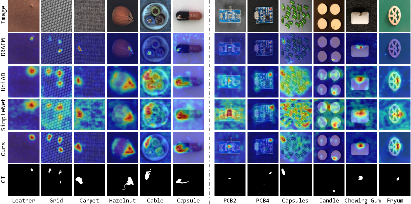
Figure 6: Qualitative visualized results for anomaly segmentation. Compared with the latest augmentation-based DRÆM [10] (2nd row), reconstruction-based UniAD [12] (3rd row), and embedding-based SimpleNet [3] (4th row) on MVTec AD [2] (Left) and VisA [35] (Right) datasets, our ViTAD (5th row) has a more accurate and compact anomaly location capability.

4.3 Quantitative Comparisons with SoTAs on VisA

As a more challenging dataset, VisA contains more complex structures, multiple and large variations of objects, and more images. In this experiment, we select one of the most advanced and powerful methods from each category for a comprehensive comparison with our ViTAD, and Tab. VII shows detailed quantitative results. Our ViTAD consistently achieves the best results. For instance, it surpasses the SoTA UniAD by ${+1.7\uparrow}$/${+0.9\uparrow}$/${+0.5\uparrow}$ on image-level metrics. Simultaneously, it obtains a score of 75.6 on the comprehensive mAD metric, exceeding the most advanced UniAD by ${+1.1\uparrow}$. This demonstrates the effectiveness of our method, as well as its excellent generalizability on different datasets.

4.4 Qualitative Comparison with SoTAs

To further evaluate the effectiveness of our proposed method, we conduct qualitative experiments to demonstrate the anomaly localization performance of different methods. As shown in Fig. 6, the left and right sides respectively display the visualization results of different methods on various object categories in MVTec AD [2] and VisA [35] datasets. It can be observed that, compared to the three SoTA representative methods (i.e., the augmentation-based DRÆM in the second row, the reconstruction-based UniAD in the third row, and the embedding-based SimpleNet in the fourth row), our method is capable of generating more accurate and compact anomaly localization, with less edge uncertainty, and exhibits fewer anomaly responses in normal areas. Taking the example of a textural Carpet with large-scale anomalies and a Capsule object with irregularly shaped anomalies, our method generates anomaly segmentation with a significantly larger intersection over union compared to the ground truth and does not produce irrelevant responses in normal areas.

4.5 Ablation and Analysis

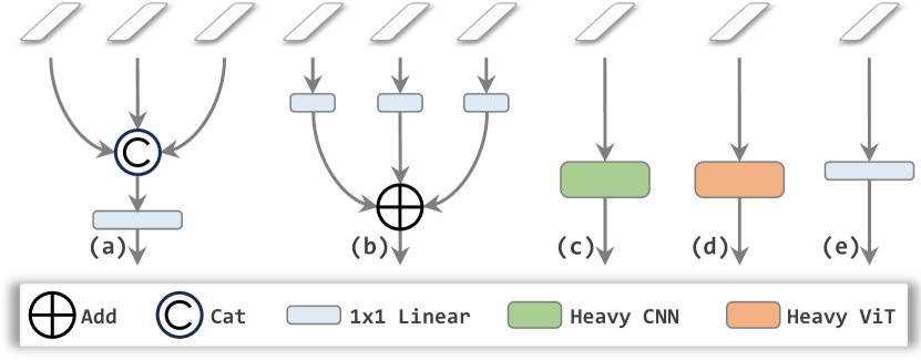
Figure 7: Structural variants of Fuser $\mathcal{F}$, which differ in input and Fuser module. (a) Only the last feature $F_{4}$; (b) Multi-scale features with concatenation; (c) Multi-scale features with addition; (d) $F_{4}$ followed by a heavy CNN-based network; (e) $F_{4}$ followed by a heavy Transformer-based network.

TABLE VIII: Quantitative evaluation of different Fuser $\mathcal{F}$ variants. The numbers in the “Add” and “Cat” rows at the top represent the usage of corresponding stage features, while the numbers in the “ViT” and “Conv” rows at the bottom denote the number of ViT [18] and BottleNeck [17] layers used respectively. Methods in blue and orange represent our ViTAD and ViTAD-C, respectively.

Fuser Variant		Image-level				Pixel-level					mAD
		mAU-ROC	mAP	m$F_{1}$-max		mAU-ROC	mAP	m$F_{1}$-max	mAU-PRO
Cat	01234	97.5	99.0	96.4		97.8	55.3	59.1	91.5		85.2
	1234	97.6	99.0	96.4		97.8	55.2	59.1	91.2		85.2
	234	97.4	98.8	96.3		97.2	54.3	57.7	91.0		84.7
	34	97.8	98.9	96.8		97.4	54.7	58.3	91.4		85.0
Add	01234	97.5	99.0	96.5		97.8	55.4	59.3	91.3		85.3
	1234	97.5	99.0	96.5		97.8	55.2	59.1	91.2		85.2
	234	97.3	98.6	96.1		97.2	54.3	58.0	90.8		84.6
	34	98.2	99.3	97.1		97.3	54.4	58.2	91.1		85.1
ViT	1	98.2	99.3	97.2		97.6	55.4	58.5	91.2		85.4
	3	98.4	99.4	97.3		97.7	55.7	58.6	91.3		85.5
	5	98.3	99.3	97.5		97.7	55.4	58.7	91.3		85.5
Conv	1	98.4	99.4	97.6		98.0	57.6	60.2	91.9		86.2
	3	97.9	99.2	97.1		98.0	57.8	60.7	91.9		86.1
	5	98.1	99.3	97.1		98.1	58.5	60.7	91.8		86.2
	ViTAD	98.3	99.4	97.3		97.7	55.3	58.7	91.4		85.4

4.5.1 Structural Variants of Fuser $\mathcal{F}$

As shown in Fig. 7, in addition to the structure described in Sec. 3.3, this paper also attempts to fuse multi-layer features (i.e., a and b in Fig. 7), as well as employs a deeper sub-model with CNN-based BottleNeck (i.e., c in Fig. 7), and ViT block (i.e., d in Fig. 7) as the input of the Decoder, aiming at exploring the impact of different layer feature fusion and model depth on the algorithm results. Tab. VIII presents the quantitative evaluation results. When more layer features are fused, it shows a slight decrease in the image-level metrics and a minor increase in the pixel-level metrics. The analysis suggests that low-level features positively contribute to pixel-level localization, but a shorter information flow can negatively affect global image classification; whereas high-level features contain more semantic information, which is more beneficial for image classification. This is slightly different from the belief in works like RD [11] and UniAD [12] that multi-scale features can stably enhance model performance. Considering model complexity and performance, this paper only uses the output feature of the last layer, i.e., $F_{4}$, as the input to the Decoder. This strikes a good balance between the accuracy and performance of the AD model. Furthermore, we explore the impact of model depth on the results of different infrastructures. Additional CNN-based structure can significantly enhance the model performance in all metrics, termed ViTAD-C in orange background. This implies that complementary basic structures can further bring additional gains for our ViTAD, even though the plain structure has already achieved impressive SoTA results. For instance, the average mAD increases from 85.4 to 86.2 (${+0.8\uparrow}$) after adding one BottleNeck layer, but more layers do not significantly improve the performance. In contrast, using ViT does not bring about a noticeable improvement in model performance. Following the principle of simple and effective structural design, this paper only uses one linear layer as the Fuser structure, i.e., (e) in Fig. 7.

4.5.2 Influence of Pre-trained ViT

Note that whether the features extracted by the encoder are discriminant against anomalies will significantly affect the performance of the studied reconstruction-based methods. Therefore, using ViT-S [18] as the backbone, we explore the impact of different pre-trained weights on the results. As shown in Tab. I, we find that the pre-trained weights are crucial for the performance: 1) We explore a randomly initialized encoder with fixed parameters as the encoder model (c.f., first row), and its results show a significant gap against using pre-trained models, proving the necessity of pre-trained weights. Interestingly, the model still has some effects in this case, such as the image-level and pixel-level mAU-ROC being higher than 0.5. The image-level mAP and mF1 are as high as 79.5 and 84.7, respectively, indicating that the lower limit of these metrics is very high. This also indirectly demonstrates the necessity and complementarity of using multiple metrics simultaneously of our suggestion in Sec. 4.1. 2) Rows 2 to 8 reveal the impact of different pre-trained models on the results, and there is a significant gap among them. For example, the mAD of DINO is ${+3.0\uparrow}$ higher than the supervised training model of ImageNet-1K, and ${+1.8\uparrow}$ higher than the self-supervised training MAE. The results based on CLIP are significantly inferior to other methods, whose training objective is to align image and text, potentially neglecting information for detailed structures. Moreover, the performance of the pre-trained model in AD has nothing to do with its corresponding classification accuracy. For instance, the classification accuracies of DINO-Small, MoCo v3-Small, and MAE-Small on ImageNet-1K are 82.8, 83.2, and 83.6 [105], respectively, but on the contrary, DINO-Small performs best among popular approaches Tab. I. 3) Based on DINO pre-trained weights, we further explore the impact of smaller patch size and higher image resolution on the results (c.f., rows 9 to 10). It can be seen that both slightly reduce the image-level indicators, but significantly increase the pixel-level indicators, such as mAU-ROC, mAP, m$F_{1}$-max, and mAU-PRO can increase by up to ${+0.6\uparrow}$, ${+11.4\uparrow}$, ${+7.0\uparrow}$, and ${+2.0\uparrow}$, and the averaged mAD increases from 85.4 to 88.1. This experiment proves that the proposed method has the promising potential for further performance improvement. Nevertheless, considering the balance between model performance and efficiency, this paper does not go deeper and will be further explored in our future works.

TABLE IX: Ablation study on model scaling. Besides DINO-Small/Base models, results of ViT trained on ImageNet-1K at different scales are also presented. Pretrained models are from tripartite TIMM of version v0.8.15dev0.

Backbone Scale		Image-level				Pixel-level					mAD
		mAU-ROC	mAP	m$F_{1}$-max		mAU-ROC	mAP	m$F_{1}$-max	mAU-PRO
ImageNet-1K	T	89.7	95.2	93.0		94.3	43.8	49.7	82.7		78.3
	S	94.4	97.5	95.3		96.6	51.6	54.5	87.2		82.4
	B	96.1	98.1	96.5		96.0	50.7	54.6	86.8		82.7
	L	94.9	97.6	94.3		94.6	45.2	49.6	85.7		80.3
	H	90.9	95.6	92.2		93.8	45.0	48.3	79.8		77.9
DINO	S	98.3	99.4	97.3		97.7	55.3	58.7	91.4		85.4
	B	97.5	99.0	96.7		97.9	55.4	58.6	90.1		85.0

4.5.3 Model Scaling Analysis

We have investigated the impact of different model scales on the results based on two training methods: supervised learning with ImageNet-1K [32] and unsupervised learning with DINO [103]. As illustrated in Tab. IX, contrary to the common consensus in standard classification, detection, and segmentation tasks, larger-scale models do not always improve AD performance. For instance, the image-level mAU-ROC of DINO-B is 0.8 lower than the smaller-scale DINO-S, and mAD is 0.4 lower. This phenomenon is also reflected in AD works such as RD [11], UniAD [12], etc. For example, when switching to a larger ResNet-152 [17] model or a more powerful Swin Transformer [94] backbone, the results are significantly inferior to those of the default backbone in the paper. This inspires us to explore the inconsistency between the trend of model accuracy growth and larger-scale models in future research.

TABLE X: Ablation study on model depth and division. $i\times j$ indicates that the network contains $i$ divisions with each owing $j$ layers for the decoder. $a-b-c$ means that the decoder has 3 divisions with $a$, $b$, and $c$ layers, respectively.

Encoder	Decoder	Image-level	Pixel-level	mAD
1 $\times$ 3	1 $\times$ 3	69.9/83.6/86.4	81.1/21.9/27.1/58.4	61.2
2 $\times$ 3	1 $\times$ 3	93.6/96.9/93.6	93.8/48.6/52.3/87.1	80.8
3 $\times$ 3	2 $\times$ 3	98.1/99.2/97.2	97.2/53.9/57.6/91.2	84.9
4 $\times$ 3	3 $\times$ 2	98.0/99.2/97.2	97.6/55.0/58.5/91.3	85.3
4 $\times$ 3	3 $\times$ 4	98.1/99.2/97.2	97.7/55.4/58.7/91.2	85.3
4 $\times$ 3	2 $-$ 3 $-$ 4	98.1/99.1/97.1	97.7/55.3/58.7/91.5	85.4
4 $\times$ 3	4 $-$ 3 $-$ 2	98.1/99.2/97.2	97.6/55.1/58.4/91.0	85.2
6 $\times$ 2	5 $\times$ 2	98.1/99.2/97.1	97.6/55.5/58.7/91.5	85.4
3 $\times$ 4	2 $\times$ 4	97.8/99.1/97.3	97.9/55.7/59.0/91.4	85.4
4 $\times$ 3	3 $\times$ 3	98.3/99.4/97.3	97.7/55.3/58.7/91.4	85.4

4.5.4 Model Depth and Division Analysis

Considering both the computational cost and performance of the model, a 12-layer ViT-S with three layers for each division is utilized for experiments, and only the last three divisions (also referred to as stages in other contexts) are employed for the decoder. In addition to this division pattern, we have also experimented with different depth and division combinations, as shown in Tab. X. 1) The top part demonstrates the impact of different depths of the encoder and decoder on the results, with shallower model depths leading to poorer performance. 2) The middle part discusses the effect of an asymmetric decoder, which is found to have a negligible impact on the results, which also indirectly demonstrates the stability and robustness of our approach. 3) The bottom part indicates that different division methods have a minimal effect on the results, as these models fully consider both deep and shallow features. For the above experiments, when using $i$ divisions in the encoder, the output of the last division is fed into the Fuser, while the outputs of other $i-1$ divisions are used as restraint features. Since the features of the first stage are not used, the number of divisions in the decoder is always one less than that in the encoder.

TABLE XI: Ablation study on different pixel-wise loss functions of different approaches. ^†: Default loss function in the paper.

Item		Image-level				Pixel-level					mAD
		mAU-ROC	mAP	m$F_{1}$-max		mAU-ROC	mAP	m$F_{1}$-max	mAU-PRO
RD	L1	93.4	97.2	95.7		95.8	46.8	52.2	90.2		81.6
	MSE	97.7	99.0	96.7		96.4	48.4	53.3	91.1		83.2
	Cosp	95.3	97.6	96.1		96.2	50.5	55.0	91.5		83.2
	Cosf †	94.6	96.5	95.2		96.1	48.6	53.8	91.2		82.3
UniAD	L1	96.6	98.7	96.5		96.8	44.4	49.7	90.2		81.8
	MSE †	97.5	99.1	97.3		97.0	45.1	50.4	90.7		82.4
	Cosp	74.6	88.1	87.9		84.1	19.1	24.6	64.2		63.2
	Cosf	76.5	89.1	88.5		82.1	18.4	24.2	62.1		63.0
ViTAD	L1	97.6	99.0	96.8		97.5	54.9	58.4	91.2		85.1
	MSE	97.7	99.1	97.0		97.6	55.0	58.6	91.5		85.2
	Cosp	98.1	99.3	97.2		97.7	55.4	58.9	91.8		85.5
	Cosf †	98.3	99.4	97.3		97.7	55.3	58.7	91.4		85.4

TABLE XII: Ablation study on training epoch, scheduler, and augmentation. CC: Center Crop. CJ: Color Jitter. RHF: Random Horizontal Flip. RR: Random Rotation. RRC: Random Resized Crop.

Item		Image-level				Pixel-level					mAD
		mAU-ROC	mAP	m$F_{1}$-max		mAU-ROC	mAP	m$F_{1}$-max	mAU-PRO
Epoch	30	97.4	99.0	96.6		97.5	55.2	58.7	91.1		85.1
	50	97.9	99.1	97.1		97.7	55.5	58.8	91.3		85.3
	100	98.3	99.4	97.3		97.7	55.3	58.7	91.4		85.4
	200	98.1	99.1	96.7		97.6	55.6	58.4	91.3		85.3
	300	98.1	99.1	96.9		97.6	55.4	58.6	91.2		85.3
Sche.	Cosine	98.0	99.0	97.1		97.7	55.5	58.7	91.2		85.3
	Step	98.3	99.4	97.3		97.7	55.3	58.7	91.4		85.4
Augmentation	CC+CJ	73.1	89.8	86.3		66.8	8.5	15.0	20.9		51.5
	CC+RHF	75.6	90.9	86.7		65.8	8.6	14.8	19.1		51.6
	CC+RR	72.1	88.9	85.7		67.0	8.6	15.1	21.0		51.2
	RRC	92.5	96.5	92.1		84.1	18.6	27.9	48.6		65.8
	All	88.3	95.0	90.3		75.9	13.2	21.7	35.9		60.0
	None	98.3	99.4	97.3		97.7	55.3	58.7	91.4		85.4

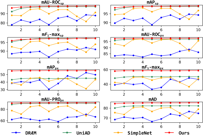
Figure 8: Stability comparison of all metrics during the training process for different methods. Each model is tested ten times at linear intervals during the training process.

4.5.5 Robustness Analyses

We evaluate the robustness of the proposed ViTAD from multiple dimensions. 1) Loss Function. Following Occam’s Razor principle, the reconstruction-based ViTAD only uses a pixel-wise loss function for model training. Specifically, we use four types of loss functions, i.e., L1, Mean Square Error (MSE), pixel-wise Cosine Similarity (Cos_p), and flattened Cosine Similarity (Cos_f), for quantitative comparison with the SoTA RD [11] and UniAD [12]. As shown in Tab. XI, our method is robust to different loss functions, with mAD showing no significant fluctuations (c.f., bottom part). RD has noticeable gaps in multiple metrics (c.f., middle part), and UniAD has significant gaps (c.f., top part) where a significant decrease in model performance when switching to any Cos_p and Cos_f. 2) Train Epoch. The convergence of the model significantly impacts its application value. The top part of Tab. XII shows the performance under different epochs. The proposed method achieves stable results at 30 epochs and optimal results at 100 epochs. Considering the balance between training resources and performance, we set the default train epoch to 100, and this number still has a significant advantage compared to the comparison methods (c.f., Sec. 4.1). 3) Train Scheduler The Cosine scheduler has been proven to have a positive effect in the fields of classification, detection, segmentation, etc. Still, no one has explored it in the AD field. Therefore, we explore its impact on our ViTAD in the middle part of Tab. XII. Results show the strong robustness of our approach to different train schedulers, but the effect of the Cosine scheduler slightly decreases compared to the Step scheduler. 4) Train Augmentation. Furthermore, the impact of 5 types of data augmentation on model training is explored in the bottom part of Tab. XII, and we find that proven effective data augmentation methods in other fields may have a negative effect in the AD field. We leave this interesting finding for future work. 5) Metric Stability During Training. When replicating comparison methods, we find that some methods have significant fluctuations in metric evaluation during training. Therefore, we analyze the fluctuations in metrics during training in several mainstream methods. As shown in Fig. 8, DRÆM [10] and SimpleNet [3] have noticeable jitters during training, while UniAD [12] and our method are very stable, but our method has significant advantages in metric results and convergence speed.

TABLE XIII: Efficiency comparison of different methods.

Method	Parameters	FLOPs	Train Memory	Train Time
DRÆM	097.4 M	198.0 G	19,852 M	19.6 H
RD	080.6 M	028.4 G	03,872 M	04.1 H
UniAD	024.5 M	003.6 G	06,844 M	13.4 H
DeSTSeg	035.2 M	122.7 G	03,562 M	02.5 H
SimpleNet	072.8 M	016.1 G	05,488 M	11.8 H
ViTAD	038.6 M	010.7 G	02,300 M	01.1 H

4.5.6 Efficiency Comparison with SoTAs

Considering practical applications, in addition to the model’s performance, we also need to evaluate the efficiency thoroughly. Specifically, we fairly evaluate the pros and cons of different methods in four dimensions: 1) the number of parameters, 2) FLOPs, 3) Train Memory, and 4) time consumption (evaluated on a single V100 GPU with a batch size of 8). Tab. XIII shows that our method has significantly smaller train memory and time consumption while having the highest evaluation metrics (c.f., Sec. 4.2 and Sec. 4.3). E.g., our ViTAD only requires 1.1 hours and 2.3G of GPU memory to complete model training while requiring very competitive parameters and FLOPs.

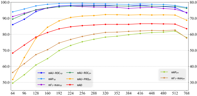
Figure 9: Analysis of model performance with varying resolutions. Pixel-level mAP_px and m$F_{1}$-max_px use the right vertical axis, while the remaining metrics share the left vertical axis.

4.5.7 Investigating Impact of Resolution

The current method defaults to conducting experiments at a resolution of 224$\times$224 [11, 3] or 256$\times$256 [10, 12, 34], and there has yet to be any AD work exploring the impact of different resolutions on model performance. Considering the practical application requirements for different resolutions, we conduct experiments at intervals of 32 pixels within an extensive range from 64$\times$64 to 512$\times$512 and additionally test the results under an extreme 768$\times$768 resolution. As shown in Fig. 9, different metric results gradually improve as the resolution increases, and the results tend to stabilize at a resolution of 256$\times$256. Interestingly, our method can still achieve satisfactory results under a very low resolution (e.g., 64$\times$64), but when the resolution is too high (e.g., 768$\times$768), the model results decline. This inspires us to research high-resolution AD tasks in the future.

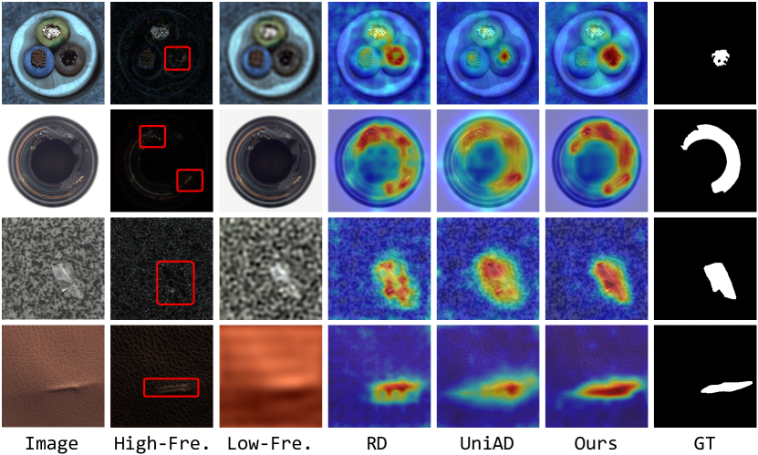
Figure 10: Comparative analysis from a frequency domain perspective. The second and third columns represent the input image’s high-/low-frequency decomposition in the first column, while the last column represents the ground truth of anomaly segmentation. The other columns display the anomaly segmentation results of different methods.

4.5.8 Advantage Explanation of ViT

Thanks to the global modeling capability of Multi-Head Self-Attention (MHSA), ViT can simultaneously pay attention to distant low-frequency information and close high-frequency information [97, 110]. That is what CNN, with the local modeling manner, does not have. At the same time, the dynamic modeling approach also endows the model with more robust generalization capabilities. As shown in Fig. 10, the second and third columns display the original image’s high- and low-frequency decomposition in the first column. It can be seen that the abnormal area is not only reflected in the low-frequency components but is also significant in the high-frequency component (c.f., red rectangular boxes). Compared to the contrast methods, our model has more accurate and compact abnormal segmentation capabilities. Whether inside the abnormality or at the edge, our ViTAD is more in line with the ground truth. This also proves the effectiveness of ViT’s multi-frequency dynamic modeling capabilities for reconstruction-based AD models.

5 Conclusion

Addressing the more challenging and practical Multi-class Unsupervised Anomaly Detection task, this paper explores the feasibility of using a plain Vision Transformer (ViT) for the first time. Specifically, we abstract a Meta-AD framework based on the current reconstruction methods, and by Occam’s Razor principle, we propose a powerful yet efficient ViTAD baseline. We propose a comprehensive and fair evaluation benchmark on eight metrics for this increasingly popular task. Surprisingly, our method achieves impressive results on popular MVTec AD and VisA datasets without inventing or introducing additional modules, datasets, or training techniques. Furthermore, we conduct thorough comparative and ablation experiments to demonstrate the effectiveness and robustness of our method and provide some interesting findings for potential further work. We hope our study will inspire future research for advancing ViT to the MUAD field and beyond.
Limitations and Future Works. This work only explores the most naive plain ViT solution for MUAD, and further investigations of AD-oriented ViT improvements and data augmentations could potentially enhance the model’s performance. Additionally, AD-specific pre-training techniques are also worth investigating.

References

- [1] J. Liu, G. Xie, J. Wang, S. Li, C. Wang, F. Zheng, and Y. Jin, “Deep industrial image anomaly detection: A survey,” arXiv preprint arXiv:2301.11514, 2023.
- [2] P. Bergmann, M. Fauser, D. Sattlegger, and C. Steger, “Mvtec ad–a comprehensive real-world dataset for unsupervised anomaly detection,” in CVPR, 2019.
- [3] Z. Liu, Y. Zhou, Y. Xu, and Z. Wang, “Simplenet: A simple network for image anomaly detection and localization,” in CVPR, 2023.
- [4] T. Fernando, H. Gammulle, S. Denman, S. Sridharan, and C. Fookes, “Deep learning for medical anomaly detection–a survey,” ACM Computing Surveys, 2021.
- [5] C. Han, L. Rundo, K. Murao, T. Noguchi, Y. Shimahara, Z. Á. Milacski, S. Koshino, E. Sala, H. Nakayama, and S. Satoh, “Madgan: Unsupervised medical anomaly detection gan using multiple adjacent brain mri slice reconstruction,” BMC Bioinformatics, 2021.
- [6] A. Kascenas, P. Sanchez, P. Schrempf, C. Wang, W. Clackett, S. S. Mikhael, J. P. Voisey, K. Goatman, A. Weir, N. Pugeault et al., “The role of noise in denoising models for anomaly detection in medical images,” Medical Image Analysis, 2023.
- [7] A. Berroukham, K. Housni, M. Lahraichi, and I. Boulfrifi, “Deep learning-based methods for anomaly detection in video surveillance: a review,” Bulletin of Electrical Engineering and Informatics, 2023.
- [8] J. Fioresi, I. R. Dave, and M. Shah, “Ted-spad: Temporal distinctiveness for self-supervised privacy-preservation for video anomaly detection,” in ICCV, 2023.
- [9] V.-T. Le and Y.-G. Kim, “Attention-based residual autoencoder for video anomaly detection,” Applied Intelligence, 2023.
- [10] V. Zavrtanik, M. Kristan, and D. Skočaj, “Draem-a discriminatively trained reconstruction embedding for surface anomaly detection,” in ICCV, 2021.
- [11] H. Deng and X. Li, “Anomaly detection via reverse distillation from one-class embedding,” in CVPR, 2022.
- [12] Z. You, L. Cui, Y. Shen, K. Yang, X. Lu, Y. Zheng, and X. Le, “A unified model for multi-class anomaly detection,” NeurIPS, 2022.
- [13] C.-L. Li, K. Sohn, J. Yoon, and T. Pfister, “Cutpaste: Self-supervised learning for anomaly detection and localization,” in CVPR, 2021.
- [14] D. Gudovskiy, S. Ishizaka, and K. Kozuka, “Cflow-ad: Real-time unsupervised anomaly detection with localization via conditional normalizing flows,” in WACV, 2022.
- [15] P. Bergmann, M. Fauser, D. Sattlegger, and C. Steger, “Uninformed students: Student-teacher anomaly detection with discriminative latent embeddings,” in CVPR, 2020.
- [16] K. Roth, L. Pemula, J. Zepeda, B. Schölkopf, T. Brox, and P. Gehler, “Towards total recall in industrial anomaly detection,” in CVPR, 2022.
- [17] K. He, X. Zhang, S. Ren, and J. Sun, “Deep residual learning for image recognition,” in CVPR, 2016.
- [18] A. Dosovitskiy, L. Beyer, A. Kolesnikov, D. Weissenborn, X. Zhai, T. Unterthiner, M. Dehghani, M. Minderer, G. Heigold, S. Gelly, J. Uszkoreit, and N. Houlsby, “An image is worth 16x16 words: Transformers for image recognition at scale,” in ICLR, 2021.
- [19] C. Zhou and R. C. Paffenroth, “Anomaly detection with robust deep autoencoders,” in KDD, 2017.
- [20] S. Akcay, A. Atapour-Abarghouei, and T. P. Breckon, “Ganomaly: Semi-supervised anomaly detection via adversarial training,” in ACCV. Springer, 2019.
- [21] Z. You, K. Yang, W. Luo, L. Cui, Y. Zheng, and X. Le, “Adtr: Anomaly detection transformer with feature reconstruction,” in ICONIP. Springer, 2022.
- [22] P. Mishra, R. Verk, D. Fornasier, C. Piciarelli, and G. L. Foresti, “Vt-adl: A vision transformer network for image anomaly detection and localization,” in ISIE. IEEE, 2021.
- [23] Y. Li, H. Mao, R. Girshick, and K. He, “Exploring plain vision transformer backbones for object detection,” in ECCV. Springer, 2022.
- [24] Y. Lin, Y. Yuan, Z. Zhang, C. Li, N. Zheng, and H. Hu, “Detr does not need multi-scale or locality design,” in ICCV, 2023, pp. 6545–6554.
- [25] S. Zheng, J. Lu, H. Zhao, X. Zhu, Z. Luo, Y. Wang, Y. Fu, J. Feng, T. Xiang, P. H. Torr et al., “Rethinking semantic segmentation from a sequence-to-sequence perspective with transformers,” in CVPR, 2021.
- [26] A. Kirillov, E. Mintun, N. Ravi, H. Mao, C. Rolland, L. Gustafson, T. Xiao, S. Whitehead, A. C. Berg, W.-Y. Lo, P. Dollar, and R. Girshick, “Segment anything,” in ICCV, 2023.
- [27] X. Wang, X. Zhang, Y. Cao, W. Wang, C. Shen, and T. Huang, “Seggpt: Segmenting everything in context,” arXiv preprint arXiv:2304.03284, 2023.
- [28] B. Zhang, Z. Tian, Q. Tang, X. Chu, X. Wei, C. Shen et al., “Segvit: Semantic segmentation with plain vision transformers,” in NeurIPS, 2022.
- [29] B. Zhang, L. Liu, M. H. Phan, Z. Tian, C. Shen, and Y. Liu, “Segvitv2: Exploring efficient and continual semantic segmentation with plain vision transformers,” arXiv preprint arXiv:2306.06289, 2023.
- [30] Y. Xu, J. Zhang, Q. Zhang, and D. Tao, “Vitpose: Simple vision transformer baselines for human pose estimation,” in NeurIPS, 2022.
- [31] ——, “Vitpose+: Vision transformer foundation model for generic body pose estimation,” arXiv preprint arXiv:2212.04246, 2022.
- [32] J. Deng, W. Dong, R. Socher, L.-J. Li, K. Li, and L. Fei-Fei, “Imagenet: A large-scale hierarchical image database,” in CVPR. Ieee, 2009.
- [33] E. Mathian, H. Liu, L. Fernandez-Cuesta, D. Samaras, M. Foll, and L. Chen, “Haloae: An halonet based local transformer auto-encoder for anomaly detection and localization,” arXiv preprint arXiv:2208.03486, 2022.
- [34] X. Zhang, S. Li, X. Li, P. Huang, J. Shan, and T. Chen, “Destseg: Segmentation guided denoising student-teacher for anomaly detection,” in CVPR, 2023.
- [35] Y. Zou, J. Jeong, L. Pemula, D. Zhang, and O. Dabeer, “Spot-the-difference self-supervised pre-training for anomaly detection and segmentation,” in ECCV. Springer, 2022.
- [36] P. Liznerski, L. Ruff, R. A. Vandermeulen, B. J. Franks, M. Kloft, and K. R. Muller, “Explainable deep one-class classification,” in ICLR, 2021.
- [37] R. Wang, S. Hoppe, E. Monari, and M. F. Huber, “Defect transfer gan: diverse defect synthesis for data augmentation,” arXiv preprint arXiv:2302.08366, 2023.
- [38] W.-H. Chu and K. M. Kitani, “Neural batch sampling with reinforcement learning for semi-supervised anomaly detection,” in ECCV. Springer, 2020.
- [39] G. Xie, J. Wang, J. Liu, Y. Jin, and F. Zheng, “Pushing the limits of fewshot anomaly detection in industry vision: Graphcore,” in ICLR, 2023.
- [40] J. Jeong, Y. Zou, T. Kim, D. Zhang, A. Ravichandran, and O. Dabeer, “Winclip: Zero-/few-shot anomaly classification and segmentation,” in CVPR, 2023.
- [41] X. Chen, Y. Han, and J. Zhang, “A zero-/few-shot anomaly classification and segmentation method for cvpr 2023 vand workshop challenge tracks 1&2: 1st place on zero-shot ad and 4th place on few-shot ad,” arXiv preprint arXiv:2305.17382, 2023.
- [42] Y. Cao, X. Xu, C. Sun, Y. Cheng, Z. Du, L. Gao, and W. Shen, “Segment any anomaly without training via hybrid prompt regularization,” arXiv preprint arXiv:2305.10724, 2023.
- [43] J. Zhang, X. Chen, Z. Xue, Y. Wang, C. Wang, and Y. Liu, “Exploring grounding potential of vqa-oriented gpt-4v for zero-shot anomaly detection,” arXiv preprint arXiv:2311.02612, 2023.
- [44] T. Hu, J. Zhang, R. Yi, Y. Du, X. Chen, L. Liu, Y. Wang, and C. Wang, “Anomalydiffusion: Few-shot anomaly image generation with diffusion model,” arXiv preprint arXiv:2312.05767, 2023.
- [45] M. Yang, P. Wu, and H. Feng, “Memseg: A semi-supervised method for image surface defect detection using differences and commonalities,” EAAI, 2023.
- [46] G. Zhang, K. Cui, T.-Y. Hung, and S. Lu, “Defect-gan: High-fidelity defect synthesis for automated defect inspection,” in WACV, 2021.
- [47] O. Rippel, P. Mertens, and D. Merhof, “Modeling the distribution of normal data in pre-trained deep features for anomaly detection,” in ICPR. IEEE, 2021.
- [48] K. Zhang, B. Wang, and C.-C. J. Kuo, “Pedenet: Image anomaly localization via patch embedding and density estimation,” PRL, 2022.
- [49] Q. Wan, L. Gao, X. Li, and L. Wen, “Unsupervised image anomaly detection and segmentation based on pretrained feature mapping,” TII, 2022.
- [50] Q. Wan, Y. Cao, L. Gao, W. Shen, and X. Li, “Position encoding enhanced feature mapping for image anomaly detection,” in CASE. IEEE, 2022.
- [51] D. Rezende and S. Mohamed, “Variational inference with normalizing flows,” in ICML. PMLR, 2015.
- [52] G. Papamakarios, E. Nalisnick, D. J. Rezende, S. Mohamed, and B. Lakshminarayanan, “Normalizing flows for probabilistic modeling and inference,” JMLR, 2021.
- [53] M. Rudolph, B. Wandt, and B. Rosenhahn, “Same same but differnet: Semi-supervised defect detection with normalizing flows,” in WACV, 2021.
- [54] J. Yu, Y. Zheng, X. Wang, W. Li, Y. Wu, R. Zhao, and L. Wu, “Fastflow: Unsupervised anomaly detection and localization via 2d normalizing flows,” arXiv preprint arXiv:2111.07677, 2021.
- [55] J. Lei, X. Hu, Y. Wang, and D. Liu, “Pyramidflow: High-resolution defect contrastive localization using pyramid normalizing flow,” in CVPR, 2023.
- [56] Q. Wan, L. Gao, X. Li, and L. Wen, “Unsupervised image anomaly detection and segmentation based on pretrained feature mapping,” TII, 2023.
- [57] Y. Cao, Q. Wan, W. Shen, and L. Gao, “Informative knowledge distillation for image anomaly segmentation,” KBS, 2022.
- [58] G. Wang, S. Han, E. Ding, and D. Huang, “Student-teacher feature pyramid matching for anomaly detection,” in BMVC, 2021.
- [59] S. Yamada, S. Kamiya, and K. Hotta, “Reconstructed student-teacher and discriminative networks for anomaly detection,” in IROS. IEEE, 2022.
- [60] N. Cohen and Y. Hoshen, “Sub-image anomaly detection with deep pyramid correspondences,” arXiv preprint arXiv:2005.02357, 2020.
- [61] T. Defard, A. Setkov, A. Loesch, and R. Audigier, “Padim: a patch distribution modeling framework for anomaly detection and localization,” in ICPR. Springer, 2021.
- [62] J. Hyun, S. Kim, G. Jeon, S. H. Kim, K. Bae, and B. J. Kang, “Reconpatch: Contrastive patch representation learning for industrial anomaly detection,” arXiv preprint arXiv:2305.16713, 2023.
- [63] W. Liu, H. Chang, B. Ma, S. Shan, and X. Chen, “Diversity-measurable anomaly detection,” in CVPR, 2023.
- [64] Z. Gu, L. Liu, X. Chen, R. Yi, J. Zhang, Y. Wang, C. Wang, A. Shu, G. Jiang, and L. Ma, “Remembering normality: Memory-guided knowledge distillation for unsupervised anomaly detection,” in ICCV, 2023.
- [65] C.-C. Tsai, T.-H. Wu, and S.-H. Lai, “Multi-scale patch-based representation learning for image anomaly detection and segmentation,” in WACV, 2022.
- [66] J. Jang, E. Hwang, and S.-H. Park, “N-pad: Neighboring pixel-based industrial anomaly detection,” in CVPR, 2023.
- [67] X. Xia, X. Pan, X. He, J. Zhang, N. Ding, and L. Ma, “Discriminative-generative representation learning for one-class anomaly detection,” arXiv preprint arXiv:2107.12753, 2021.
- [68] G. Kwon, M. Prabhushankar, D. Temel, and G. AlRegib, “Backpropagated gradient representations for anomaly detection,” in ECCV. Springer, 2020.
- [69] Y. Teng, H. Li, F. Cai, M. Shao, and S. Xia, “Unsupervised visual defect detection with score-based generative model,” arXiv preprint arXiv:2211.16092, 2022.
- [70] A. Mousakhan, T. Brox, and J. Tayyub, “Anomaly detection with conditioned denoising diffusion models,” arXiv preprint arXiv:2305.15956, 2023.
- [71] D. Gong, L. Liu, V. Le, B. Saha, M. R. Mansour, S. Venkatesh, and A. v. d. Hengel, “Memorizing normality to detect anomaly: Memory-augmented deep autoencoder for unsupervised anomaly detection,” in ICCV, 2019.
- [72] N. Madan, N.-C. Ristea, R. T. Ionescu, K. Nasrollahi, F. S. Khan, T. B. Moeslund, and M. Shah, “Self-supervised masked convolutional transformer block for anomaly detection,” arXiv preprint arXiv:2209.12148, 2022.
- [73] A. Bauer, “Self-supervised training with autoencoders for visual anomaly detection,” arXiv preprint arXiv:2206.11723, 2022.
- [74] J. Pirnay and K. Chai, “Inpainting transformer for anomaly detection,” in ICIAP. Springer, 2022.
- [75] Y. Liang, J. Zhang, S. Zhao, R. Wu, Y. Liu, and S. Pan, “Omni-frequency channel-selection representations for unsupervised anomaly detection,” IEEE TIP, 2023.
- [76] S. Mei, H. Yang, and Z. Yin, “An unsupervised-learning-based approach for automated defect inspection on textured surfaces,” TIM, 2018.
- [77] V. Zavrtanik, M. Kristan, and D. Skočaj, “Dsr–a dual subspace re-projection network for surface anomaly detection,” in ECCV. Springer, 2022.
- [78] H. He, J. Zhang, H. Chen, X. Chen, Z. Li, X. Chen, Y. Wang, C. Wang, and L. Xie, “Diad: A diffusion-based framework for multi-class anomaly detection,” arXiv preprint arXiv:2312.06607, 2023.
- [79] T. Schlegl, P. Seeböck, S. M. Waldstein, U. Schmidt-Erfurth, and G. Langs, “Unsupervised anomaly detection with generative adversarial networks to guide marker discovery,” in IPMI. Springer, 2017.
- [80] S. Akçay, A. Atapour-Abarghouei, and T. P. Breckon, “Skip-ganomaly: Skip connected and adversarially trained encoder-decoder anomaly detection,” in IJCNN. IEEE, 2019.
- [81] S. Deng, Z. Sun, R. Zhuang, and J. Gong, “Noise-to-norm reconstruction for industrial anomaly detection and localization,” arXiv preprint arXiv:2307.02836, 2023.
- [82] V. Zavrtanik, M. Kristan, and D. Skočaj, “Reconstruction by inpainting for visual anomaly detection,” PR, 2021.
- [83] J. Song, K. Kong, Y.-I. Park, S.-G. Kim, and S.-J. Kang, “Anomaly segmentation network using self-supervised learning,” in AAAI 2022 Workshop on AI for Design and Manufacturing (ADAM), 2022.
- [84] T. D. Tien, A. T. Nguyen, N. H. Tran, T. D. Huy, S. Duong, C. D. T. Nguyen, and S. Q. Truong, “Revisiting reverse distillation for anomaly detection,” in CVPR, 2023.
- [85] X. Jiang, J. Liu, J. Wang, Q. Nie, K. Wu, Y. Liu, C. Wang, and F. Zheng, “Softpatch: Unsupervised anomaly detection with noisy data,” NeurIPS, 2022.
- [86] H. Yao and X. Wang, “Generalizable industrial visual anomaly detection with self-induction vision transformer,” arXiv preprint arXiv:2211.12311, 2022.
- [87] Y. Zhao, “Omnial: A unified cnn framework for unsupervised anomaly localization,” in CVPR, 2023.
- [88] Y. Lee, H. Lim, and H. Yoon, “Selformaly: Towards task-agnostic unified anomaly detection,” arXiv preprint arXiv:2307.12540, 2023.
- [89] P. Bergmann, S. Löwe, M. Fauser, D. Sattlegger, and C. Steger, “Improving unsupervised defect segmentation by applying structural similarity to autoencoders,” in VISIGRAPP, 2019.
- [90] Y. Lee and P. Kang, “Anovit: Unsupervised anomaly detection and localization with vision transformer-based encoder-decoder,” Access, 2022.
- [91] A. Vaswani, N. Shazeer, N. Parmar, J. Uszkoreit, L. Jones, A. N. Gomez, Ł. Kaiser, and I. Polosukhin, “Attention is all you need,” NeurIPS, 2017.
- [92] H. Touvron, M. Cord, M. Douze, F. Massa, A. Sablayrolles, and H. Jégou, “Training data-efficient image transformers & distillation through attention,” in ICML. PMLR, 2021.
- [93] W. Wang, E. Xie, X. Li, D.-P. Fan, K. Song, D. Liang, T. Lu, P. Luo, and L. Shao, “Pyramid vision transformer: A versatile backbone for dense prediction without convolutions,” in ICCV, 2021.
- [94] Z. Liu, Y. Lin, Y. Cao, H. Hu, Y. Wei, Z. Zhang, S. Lin, and B. Guo, “Swin transformer: Hierarchical vision transformer using shifted windows,” in ICCV, 2021.
- [95] Z. Liu, H. Hu, Y. Lin, Z. Yao, Z. Xie, Y. Wei, J. Ning, Y. Cao, Z. Zhang, L. Dong et al., “Swin transformer v2: Scaling up capacity and resolution,” in CVPR, 2022.
- [96] J. Zhang, C. Xu, J. Li, W. Chen, Y. Wang, Y. Tai, S. Chen, C. Wang, F. Huang, and Y. Liu, “Analogous to evolutionary algorithm: Designing a unified sequence model,” NeurIPS, 2021.
- [97] J. Zhang, X. Li, Y. Wang, C. Wang, Y. Yang, Y. Liu, and D. Tao, “Eatformer: Improving vision transformer inspired by evolutionary algorithm,” arXiv preprint arXiv:2206.09325, 2022.
- [98] J. Zhang, X. Li, J. Li, L. Liu, Z. Xue, B. Zhang, Z. Jiang, T. Huang, Y. Wang, and C. Wang, “Rethinking mobile block for efficient attention-based models,” in ICCV, 2023.
- [99] X. Li, H. Ding, W. Zhang, H. Yuan, G. Cheng, P. Jiangmiao, K. Chen, Z. Liu, and C. C. Loy, “Transformer-based visual segmentation: A survey,” arXiv pre-print, 2023.
- [100] J. Wu, X. Li, S. X. H. Yuan, H. Ding, Y. Yang, X. Li, J. Zhang, Y. Tong, X. Jiang, B. Ghanem et al., “Towards open vocabulary learning: A survey,” arXiv preprint arXiv:2306.15880, 2023.
- [101] X. Li, J. Zhang, Y. Yang, G. Cheng, K. Yang, Y. Tong, and D. Tao, “Sfnet: Faster and accurate semantic segmentation via semantic flow,” IJCV, 2023.
- [102] K. He, H. Fan, Y. Wu, S. Xie, and R. Girshick, “Momentum contrast for unsupervised visual representation learning,” in CVPR, 2020.
- [103] M. Caron, H. Touvron, I. Misra, H. Jégou, J. Mairal, P. Bojanowski, and A. Joulin, “Emerging properties in self-supervised vision transformers,” in ICCV, 2021.
- [104] A. Radford, J. W. Kim, C. Hallacy, A. Ramesh, G. Goh, S. Agarwal, G. Sastry, A. Askell, P. Mishkin, J. Clark et al., “Learning transferable visual models from natural language supervision,” in ICML, 2021.
- [105] K. He, X. Chen, S. Xie, Y. Li, P. Dollár, and R. Girshick, “Masked autoencoders are scalable vision learners,” in CVPR, 2022.
- [106] T.-Y. Lin, M. Maire, S. Belongie, J. Hays, P. Perona, D. Ramanan, P. Dollár, and C. L. Zitnick, “Microsoft coco: Common objects in context,” in ECCV. Springer, 2014.
- [107] M. Tan and Q. Le, “Efficientnet: Rethinking model scaling for convolutional neural networks,” in ICML. PMLR, 2019.
- [108] L. Chen, Z. You, N. Zhang, J. Xi, and X. Le, “Utrad: Anomaly detection and localization with u-transformer,” Neural Networks, 2022.
- [109] W. Kim, B. Son, and I. Kim, “Vilt: Vision-and-language transformer without convolution or region supervision,” in ICML. PMLR, 2021.
- [110] C. Si, W. Yu, P. Zhou, Y. Zhou, X. Wang, and S. Yan, “Inception transformer,” NeurIPS, 2022.
- [111] Y. Wang, J. Peng, J. Zhang, R. Yi, Y. Wang, and C. Wang, “Multimodal industrial anomaly detection via hybrid fusion,” in CVPR, 2023.
- [112] R. Chen, G. Xie, J. Liu, J. Wang, Z. Luo, J. Wang, and F. Zheng, “Easynet: An easy network for 3d industrial anomaly detection,” in ACM MM, 2023.
- [113] X. Chen, J. Zhang, G. Tian, H. He, W. Zhang, Y. Wang, C. Wang, Y. Wu, and Y. Liu, “Clip-ad: A language-guided staged dual-path model for zero-shot anomaly detection,” arXiv preprint arXiv:2311.00453, 2023.
- [114] P. Bergmann, K. Batzner, M. Fauser, D. Sattlegger, and C. Steger, “The mvtec anomaly detection dataset: a comprehensive real-world dataset for unsupervised anomaly detection,” IJCV, 2021.
- [115] I. Loshchilov and F. Hutter, “Decoupled weight decay regularization,” in ICLR, 2019.