Current-controlled chirality dynamics in a mesoscopic magnetic domain wall

Abstract

We show that the chirality as internal degree of freedom of a mesoscopic domain wall inside a quasi-one-dimensional fixture can be controlled by spin-polarized current for ferro- as well as antiferromagnetic domain walls, and for recently discovered novel class of magnetic materials - altermagnets - chirality switching can be driven by usual (unpolarized) charge current. Further, we show that the current density required for the chirality manipulation can be significantly reduced in the low-temperature regime if the chirality dynamics is essentially quantum. In the quantum regime, weak currents can excite Bloch oscillations of the domain wall angular rotation velocity with the frequency proportional to the current, modulated by a much higher magnon-range frequency. A controlled switching between different chiral states is possible as well.

I Introduction

The last decade has witnessed great theoretical and experimental progress in spintronics, significantly extending our capabilities of generation, control, manipulation, and detection of spin textures by current (see, e.g., [1, 2]). This progress is in particular driven by rich possibilities offered by effects of spin-orbit coupling [3, 1] and fast magnetization dynamics in antiferromagnets [4, 5, 6, 2, 7, 8], with realization of all-electric fast switching [9, 10, 11] bearing promise for non-volatile storage operating in terahertz domain. In altermagnets, recently discovered class of magnetic materials that combine time-reversal symmetry breaking with collinear antiferromagnetic spin order, large non-relativistic spin-momentum coupling opens avenues to efficient spin current injection, robust giant magnetoresistance and other nontrivial effects [12, 13, 14, 15].

As the physics of magnetic and spintronic devices advances towards ever smaller scales, the spin textures, usually considered as classical fields, can acquire quantum behavior. Those quantum aspects received a good deal of attention in the past, in the context of the quantum tunneling of spin in magnetic nanoparticles [16], molecular clusters [17], and topologically nontrivial magnetic textures [18]. Understanding the quantum dynamics of spin textures interacting with spin or charge currents would provide a foundation for merging and hybridizing quantum and classical computing technologies.

In this paper, we study the interaction of current with a magnetic domain wall localized inside a nanosized quasi-one-dimensional structure (wire, stripe, constriction, etc). Classically, such a magnetic domain wall has an internal degree of freedom, chirality, characterizing the way of rotation of magnetization inside the wall. Two states with opposite chirality are equivalent in energy, and there is generally a finite tunneling amplitude mixing the two states and lifting the degeneracy [19, 20, 21, 22, 23].

It has been previously shown [24, 25] that for domain walls in ferromagnets (FM) and antiferromagnets (AF), spin-polarized current directly couples to the chirality degree of freedom, and the corresponding torque can drive chirality oscillations. Here we revisit this problem and demonstrate that in AF and in altermagnets (AM), in the low-temperature regime when the chirality dynamics acquires quantum features, the current density required for efficient manipulation of chirality can be significantly reduced in comparison with the classical regime realized at high temperatures. We further show that in AM, in the contrast to other magnets, chirality can be manipulated by the usual non-polarized charge current.

II Model: domain wall in a nanowire

Consider a domain wall (DW) localized by some pinning potential inside a magnetic nanowire as shown in Fig. 1. We will study ferromagnetic as well as antiferromagnetic DWs, describing the respective order parameter by the unit vector field $\bm{n}$. We assume the presence of a biaxial anisotropy, with the anisotropy energy per unit cell

$$w_{a}=S^{2}(K_{1}n_{x}^{2}+K_{2}n_{y}^{2}),$$ (1)

where $S$ denotes the underlying spin of magnetic atoms, and the anisotropy constants $K_{1}>K_{2}>0$, so $z$ is the easy axis and $x$ the hard axis. Such a DW has two equivalent states that differ by the sense of rotation of $\bm{n}$ inside the $(yz)$ easy plane.

II.1 Ferromagnetic domain wall

In the case of a FM, $\bm{n}$ is the unit vector of magnetization, and the system is described by the Lagrangian

$$\mathcal{L} = -\frac{N_{\perp}\hbar S}{a}\int dz\big{(}\bm{A}\cdot\partial_{t}\bm{n}\big{)}-W[\bm{n}]-U_{\text{pin}}$$ (2)

$$W[\bm{n}] = \frac{N_{\perp}S^{2}}{a}\int dz\Big{\{}\frac{Ja^{2}}{2}(\partial_{z}\bm{n})^{2}+K_{1}n_{x}^{2}+K_{2}n_{y}^{2}\Big{\}},$$

where $J$ is the exchange coupling, $N_{\perp}$ is the number of magnetic atoms in the cross-section of the wire, $U_{\text{pin}}$ is the pinning potential, and $a$ is the magnetic lattice constant along the direction of the wire. We also denote the cross-section area by $C_{\perp}$, and the volume of magnetic unit cell by $V_{0}$, then $C_{\perp}a=N_{\perp}V_{0}$. The vector $\bm{A}$ has the form of the vector potential of the Dirac monopole [26],

$$\bm{A}(\bm{n}_{0},\bm{n})=\frac{(\bm{n}_{0}\times\bm{n})}{1+(\bm{n}_{0}\cdot\bm{n})},\quad\bm{n}\cdot\text{rot}_{\bm{n}}\bm{A}=1.$$ (3)

The direction of the “Dirac string” given by the unit vector $\bm{n}_{0}$ can be chosen arbitrarily, and equations of motion as well as other physical quantities do not depend on the choice of $\bm{n}_{0}$ [26]. In what follows, we choose $\bm{n}_{0}=\hat{\bm{z}}$ along the easy axis.

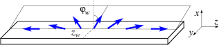
Figure 1: (Color online). Schematic picture of the mesoscopic domain wall in a quasi-one-dimensional fixture. Arrows show the direction of the magnetic order parameter (magnetization or the Néel vector).

It is convenient to use the standard spherical angles parametrization for the unit vector $\bm{n}$,

$$n_{x}+in_{y}=\sin\theta e^{i\varphi},\quad n_{z}=\cos\theta.$$

The Landau-Lifshitz equation admits the well-known Walker’s solution [27] for a DW moving with velocity $v$, with the magnetization rotating in the plane determined by the velocity-dependent angle $\phi_{0}$:

$$\theta=\theta_{0}(\xi=z-vt),\quad\varphi=\phi_{0},$$

$$\cos\theta_{0}(\xi)=\tanh\Big{(}\frac{\xi(1+\rho\cos^{2}\phi_{0})^{1/2}}{\delta}\Big{)},$$ (4)

$$\frac{v\hbar}{aS(K_{2}J)^{1/2}}=\frac{\rho\sin\phi_{0}\cos\phi_{0}}{(1+\rho\cos^{2}\phi_{0})^{1/2}},\quad\delta=a\sqrt{\frac{J}{2K_{2}}}$$

The DW described by Eq. (II.1) has the energy

$$E_{W}=N_{\perp}E_{0}\sqrt{1+\rho\cos^{2}\phi_{0}},\quad E_{0}=2S^{2}\sqrt{2JK_{2}}$$ (5)

so the lowest-energy solutions with $\phi_{0}=\pm\pi/2$ describe static DWs with opposite chirality. Here $\delta$ is the thickness of the lowest-energy DW, and $\rho$ is the rhombicity parameter indicating how much the anisotropy deviates from the uniaxial one:

$$\rho=(K_{1}-K_{2})/K_{2}.$$ (6)

Building on Walker’s solution, one can introduce collective coordinates $z_{w}(t)$, $\phi_{w}(t)$ of the DW via the ansatz [22]

$$\theta=\theta_{0}\big{(}z-z_{w}(t)\big{)},\quad\varphi=\phi_{w}(t).$$ (7)

Electrons interacting with an inhomogeneous magnetization texture experience a fictitious “gauge field” caused by the texture gradients which couples to spin current [28, 29, 30]. Performing a unitary transformation rotating the spin quantization axis of conduction electrons from its initial value (assumed to be $\bm{n}_{0}$) to the local magnetization direction $\bm{n}$ leads, to the first order in the magnetization space-time gradients, to the following contribution to the Lagrangian (2):

$$\mathcal{L}\mapsto\mathcal{L}-2C_{\perp}\int dz\,\left(\bm{j}^{(s)}\cdot\bm{\mathcal{A}}_{z}+\bm{\tau}^{(s)}\cdot\bm{\mathcal{A}}_{t}\right).$$ (8)

Here $\bm{j}^{(s)}$ is the density of the spin current along the wire direction, and $\bm{\tau}^{(s)}$ is the spin density of the conduction electrons in the locally rotated frame (i.e., with respect to the order parameter), and $\bm{\mathcal{A}}_{\mu}$ is the fictitious gauge field,

$$\bm{\mathcal{A}}_{\mu}=(\bm{e}\times\partial_{\mu}\bm{e}),$$ (9)

where unit vector $\bm{e}$ bisects the angle between $\bm{n}$ and $\bm{n}_{0}$. We assume that the exchange coupling between conduction electrons and localized spins is strong enough so the electron spin adiabatically follows the direction of the magnetization (so the coupling (8) corresponds to the adiabatic spin-transfer torque). Then in the locally rotated frame $\bm{j}^{(s)}=j^{(s)}\hat{\bm{z}}$ and $\bm{\tau}^{(s)}=\tau^{(s)}\hat{\bm{z}}$, so one can recast the current-induced contribution (8) as

$$\mathcal{L}\mapsto\mathcal{L}-I^{(s)}P_{z}-\mathcal{T}^{(s)}P_{0},\quad P_{\mu}=\int dz\,\bm{A}(\hat{\bm{z}},\bm{n})\cdot\partial_{\mu}\bm{n},$$ (10)

where $I^{(s)}=j^{(s)}C_{\perp}$, $\mathcal{T}^{(s)}=\tau^{(s)}C_{\perp}$. The integral $P_{0}$ is of the same form as the first term in the Lagrangian (2), so in a FM the second contribution in (8) leads just to a slight renormalization of the characteristic time sacle and can be neglected. The integral $P_{z}$ can be rewritten as $P_{z}=\int\bm{A}\cdot d\bm{n}$. While $P_{z}$ itself is not a well-defined quanity, the difference of $P_{z}$ values for two domain walls with $\varphi=\phi_{1}$ and $\varphi=\phi_{2}$ is uniquely defined [31] since it can be expressed as the surface integral $\int dS\,(\bm{n}\cdot\text{rot}_{\bm{n}}\bm{A})$ over the spherical wedge of the $\bm{n}$ unit sphere, bounded by the semidisks $\varphi=\phi_{1,2}$. In view of (3) this latter quantity is just equal to the surface $2(\phi_{1}-\phi_{2})$ of the wedge. Thus, up to an irrelevant constant, we can set

$$P_{z}=2\phi_{w}.$$ (11)

Substituting the ansatz (7) into Eq. (2) we finally obtain the DW Lagrangian in the collective coordinates approximation:

$$\mathcal{L}_{FM} = \frac{2N_{\perp}\hbar S}{a}z_{w}\frac{d\phi_{w}}{dt}-N_{\perp}E_{0}\big{(}1+\rho\cos^{2}\phi_{w}\big{)}^{1/2}$$ (12)

$$- 2I^{(s)}\phi_{w}-\frac{Gz_{w}^{2}}{2},$$

where the last term corresponding to the pinning potential $U_{\text{pin}}$ is assumed to be of the simplest quadratic form. The canonically conjugate momentum to angle $\phi_{w}$ is

$$P_{\phi}=\frac{2N_{\perp}\hbar S}{a}z_{w},$$ (13)

so the corresponding Hamiltonian is

$$\mathcal{H}_{FM}=\frac{P_{\phi}^{2}}{2M_{\phi}}+N_{\perp}E_{0}\big{(}1+\rho\cos^{2}\phi_{w}\big{)}^{1/2}+2I^{(s)}\phi_{w},$$ (14)

where

$$M_{\phi}=\frac{(2N_{\perp}\hbar S)^{2}}{Ga^{2}}$$ (15)

plays the role of the effective moment of inertia of the DW. In the absence of current, small oscillations of the pinned DW around the equilibrium (given by $z_{w}=0$, $\phi_{w}=\pm\pi/2$) have the frequency

$$\Omega_{0}=(N_{\perp}E_{0}\rho/M_{\phi})^{1/2}.$$ (16)

II.2 Antiferromagnetic domain wall

In the case of an AF, $\bm{n}$ is the unit Néel vector, and its dynamics is described by the Lagrangian of the nonlinear sigma-model

$$\mathcal{L}=\frac{1}{2c^{2}}N_{\perp}JS^{2}a\int dz\,(\partial_{t}\bm{n})^{2}-W[\bm{n}]-U_{\text{pin}},$$ (17)

where $c$ is the limiting velocity of spin waves. For weak rhombicity $\rho\ll 1$, collective coordinates for the DW can be introduced based on the known static solution:

$$\cos\theta=\tanh\Big{(}\frac{z-z_{w}(t)}{\delta}\Big{)},\quad\varphi=\phi_{w}(t).$$ (18)

The spin-transfer torque caused by the interaction of conduction electrons with the AF spin texture can be derived in a way very similar to the FM case [28, 32], and the corresponding contribution to the Lagrangian has the same form (10). In the AF case the contribution proportional to $P_{0}$ is not merely renormalizing the already existing term and thus cannot be ignored [24]. We remark that the more rigorous derivation [33, 24], properly taking into account the non-orthogonality of orbital wave functions of electron subbands, leads to the additional overall factor $(1-\zeta^{2})$ where the parameter $\zeta$ is proportional to the ratio $t/J_{sd}$ of the electron hopping (bandwidth) $t$ to the exchange coupling $J_{sd}$ between conduction electrons and localized spins. We assume that $\zeta\ll 1$ and ignore this factor for the sake of simplicity.

Feeding (10) into (17), we obtain the effective Langangian of the DW

$$L_{AF} = \frac{N_{\perp}E_{0}}{2c^{2}}\left\{\Big{(}\frac{dz_{w}}{dt}\Big{)}^{2}+\delta^{2}\Big{(}\frac{d\phi_{w}}{dt}\Big{)}^{2}\right\}$$ (19)

$$- N_{\perp}E_{0}\Big{(}1+\frac{1}{2}\rho\cos^{2}\phi_{w}\Big{)}-\frac{Gz_{w}^{2}}{2}$$

$$- 2I^{(s)}\phi_{w}+2\mathcal{T}^{(s)}z_{w}\frac{d\phi_{w}}{dt},$$

For spin-polarized current, both the spin current $I^{(s)}$ and the spin density $\mathcal{T}^{(s)}$ are proportional to the amplitude of the electric current $I^{(c)}$:

$$I^{(s)}=\frac{\hbar\cal{P}}{2e}I^{(c)},\quad\mathcal{T}^{(s)}\simeq\frac{I^{(s)}}{v_{s}}$$ (20)

where $\cal{P}$ is the degree of spin polarization of the electric current and $v_{s}$ is the effective electron velocity which is estimated to be in the range of $1$ to $100$ km/s [24].

For strong pinning, when the characteristic frequency

$$\Omega_{\text{pin}}=(Gc^{2}/N_{\perp}E_{0})^{1/2}$$ (21)

of $z_{w}$ oscillations is much larger than the corresponding frequency

$$\omega_{0}=(E_{0}/\hbar S)\sqrt{\rho}.$$ (22)

of oscillations of the DW angle around equilibrium points $\phi_{w}=\pm\pi/2$ , the DW coordinate can be treated as “slave” and integrated out, $z_{w}\simeq(2\mathcal{T}^{(s)}/G)(d\phi_{w}/dt)$, which leads just to a slight renormalization of the limiting spin wave velocity $c$. For any pinning, since the last term in (19) can be recast in the equivalent form $-2\mathcal{T}^{(s)}\phi_{w}\frac{dz_{w}}{dt}$, it is easy to see that it contains the additional parameter $v_{s}^{-1}(dz_{w}/dt)$ compared to the last but one term in the same expression. Thus, in contrast to the FM case, for small rhombicity $\rho\ll 1$ the translational motion of the AF domain wall (dynamics of $z_{w}$) is only weakly coupled to its chirality (dynamics of $\phi_{w}$), and this coupling can be neglected for small DW velocities $dz_{w}/dt\ll c,v_{s}$.

The Hamiltonian describing the $\phi_{w}$ dynamics in an AF DW can thus be written as

$$\mathcal{H}_{AF}=\frac{p_{\phi}^{2}}{2m_{\phi}}+N_{\perp}E_{0}\Big{(}1+\frac{1}{2}\rho\cos^{2}\phi_{w}\Big{)}+2I^{(s)}\phi_{w},$$ (23)

where

$$m_{\phi}=N_{\perp}E_{0}(\delta/c)^{2}$$ (24)

is the effective moment of inertia, and $p_{\phi}=m_{\phi}(d\phi_{w}/dt)$ is the momentum canonically conjugate to $\phi_{w}$.

Figure 2: (Color online). Illustration of the toy model of altermagnet described by Eq. (25). Arrows denote localized spins, and the dashed line indicates the magnetic unit cell.

II.3 Domain wall in an altermagnet

The low-energy spin dynamics in an altermagnet in the leading approximation is described by the same nonlinear sigma-model as in the antiferromagnetic case (we neglect slight corrections caused by the back action of the electron subsystem on the magnetization). However, one can show that, in contrast to the FM or AF, in an altermagnet the gradient of the AF order parameter couples not only to spin current, but to the charge current as well. This can be easily seen on the example of the simplest tight-binding models of an altermagnet [12], described by the Hamiltonian

$$H=\sum_{\langle ll^{\prime}\rangle}\Big{\{}-t\psi_{l}^{\dagger}\psi_{l^{\prime}}-t^{\prime}\psi_{l}^{\dagger}(\bm{\sigma}\cdot\bm{S}_{ll^{\prime}})\psi_{l^{\prime}}+\text{h.c.}\Big{\}},$$ (25)

where $l$ labels sites on a square lattice, $t$ and $t^{\prime}$ are the amplitudes of spin-independent and spin-dependent hopping, respectively, and localized spins $\bm{S}_{ll^{\prime}}$ sit in the middle of the links between nearest neighbor pairs $\langle ll^{\prime}\rangle$, as shown in Fig. 2. Although this toy model is just one of the possible realizations of an altermagnet, it allows us to capture the essential physics of AMs, so we expect the final results to remain qualitatively correct in the general case.

Introducing in each unit cell the magnetization $\bm{m}$ and the Néel vector $\bm{n}$ in a standard way, and rotating the electron quantization axes to the local Néel vector direction, one can see that the spin-independent hopping again yields the coupling of texture gradients to the spin current as given by Eq. (8), while the spin-dependent hopping leads to the following contribution to the Lagrangian density in the continuum approximation:

$$-\kappa\frac{\hbar}{2e}\bm{A}(\hat{\bm{z}},n)\cdot\Big{(}j^{(c)}_{x}\partial_{x}\bm{n}-j^{(c)}_{y}\partial_{y}\bm{n}\Big{)},$$ (26)

where $\kappa=t^{\prime}/t$ is the relative strength of the spin-dependent hopping, and $\bm{j}^{(c)}$ is the density of the charge current, see (57) and the corresponding derivation in the Appendix.

Thus, in the DW setup as considered in the previous subsections, with the nanowire oriented along along one of the directions $x$ or $y$, with an electric current of the magnitude $I^{(c)}$ and spin-polarization $\mathcal{P}$ flowing along the nanowire, one obtains the Hamiltonian of the form (23), with the replacement

$$I^{(}s))\mapsto\frac{\hbar I^{(c)}}{2e}(\mathcal{P}\pm\kappa).$$ (27)

III Classical and quantum chirality control

In what follows, we focus on the case of the weak rhombicity $\rho\ll 1$, which admits the simplified description of the DW dynamics in terms of collective coordinates (the angle $\phi_{w}$ and its conjugate momentum $p$). Then, in all setups considered above the DW is described by the effective Hamiltonian of the following form:

$$\mathcal{H}=\frac{p^{2}}{2m}+\frac{1}{2}m\omega^{2}\cos^{2}\phi_{w}+b\phi_{w},$$ (28)

where the moment of inertia $m$ and the frequency $\omega$ are given by $m=M_{\phi}$, $\omega=\Omega_{0}$ for FM, , see Eqs. (15), (16), and $m=m_{\phi}$, $\omega=\omega_{0}$ for AF/AM, see Eqs. (24), (22). The Hamiltonian (28) describes a planar rotator in a two-well potential, driven by the torque $b=\gamma\hbar I^{(c)}/e$ that is proportional to the current $I_{c}$, with the coefficient $\gamma=\mathcal{P}$ for FM and AF, and $\gamma=\mathcal{P}\pm\kappa$ for AM. The quantized form of the above Hamiltonian is easily obtained by promoting the conjugate momentum to operator $\hat{p}=-i\hbar\partial/\partial\phi_{w}$.

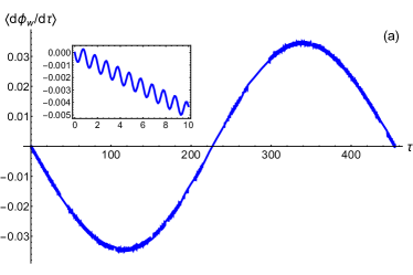
Figure 3: (Color online). The average angular velocity $\langle d\phi_{w}/d\tau\rangle$ vs the dimensionless time $\tau=\hbar t/2m$ for $\xi=5$, and bias (a) $b=0.1\Delta$; (b) $b=0.6\Delta$. The ground state for $b=0$ has been used as the initial state at $t=0$. The energies of the first four lowest-lying states at $\xi=5$ in units of $\hbar^{2}/2m$ are $E_{0}\approx 0.115$, $E_{1}\approx 0.159$, $E_{2}\approx 5.636$, and $E_{3}\approx 6.343$. Bloch oscillations with the frequency $\pi b\hbar$ are modulated with the secondary frequency $(E_{3}-E_{0})/\hbar$ due to the excitation of the third excited state.

It is convenient to introduce the dimensionless parameter

$$\xi={2m\omega}/{\hbar}$$ (29)

which determines the structure of the spectrum in the absence of the torque ($b=0$). For $\xi\gg 1$ one has the regime of “deep wells”, with the low-energy spectrum being essentially that of a tunnel-split double harmonic oscillator with the level spacing $\hbar\omega$. In this regime, both the lowest-level tunnel splitting $\Delta$ and the harmonic oscillator level spacing $\hbar\omega$ can be related to the barrier height

$$U=\frac{m\omega^{2}}{2}=\frac{1}{2}\rho E_{0}N_{\perp}$$ (30)

via the parameter $\xi$ as follows [34]:

$$\hbar\omega=\frac{4U}{\xi},\quad\Delta=Uf(\xi),\quad f(\xi)=16\left(\frac{2}{\pi\xi}\right)^{1/2}e^{-\xi}.$$ (31)

For energies considerably above $U$, the spectrum approximately corresponds to that of a free plane rotator. Decreasing $\xi$ pushes levels up, so that, e.g., for $\xi\sim 2.5\div 4$ only two lowest levels correspond to bound states inside the double well, and for $\xi\ll 1$ the entire spectrum is comprised by rotator-like delocalized states.

Applying a constant or time-dependent torque, one can excite the DW chiral degree of freedom in various ways. Depending on the parameters, this control of chirality can occur in a classical or quantum regime.

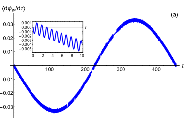
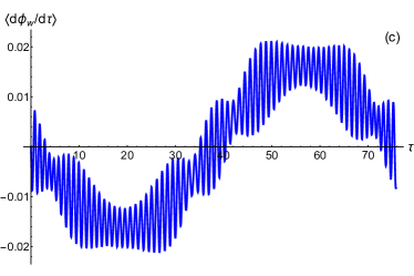
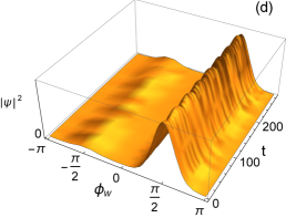
Figure 4: (Color online). Chirality dynamics with the Wannier state localized in the right well used as the initial state at $t=0$. Shown are: (a), (c) the average angular velocity $\langle d\phi_{w}/d\tau\rangle$, and (b), (d) the probability density $|\psi|^{2}$ as functions of the dimensionless time $\tau=\hbar t/2m$ for $\xi=5$. The bias is $b=0.1\Delta$ in (a), (b), and $b=0.6\Delta$ in (c), (d) .

III.1 Classical chirality dynamics

Classically, the DW is “stuck” in one of the wells, and would be driven out only by a sufficiently large torque $b>b_{c}$, when the energy gain on traversing between wells minima becomes comparable to the barrier height, $b_{c}\pi\simeq U$. The threshold current density $j^{(c)}=I^{(c)}/C_{\perp}$, neccessary for such a switching, is given by

$$j^{cl}=\frac{eE_{0}}{2\pi\hbar a^{2}}\rho$$ (32)

and does not depend on the number of spins $N_{\perp}$ in the cross-section. The physics of this regime is essentially the same for FM, AF, and AM, and has been studied in [25] for the AF case.

A constant current above the threshold will lead to accelerated precession of the DW angle. The presence of a finite damping $\eta$, will lead to a rotation with a stationary average angular velocity $\bar{\omega}\simeq b/\hbar\eta$, with superimposed oscillations with the frequency $2\bar{\omega}$, so such a setup can have applications as a nano-oscillator [35, 25]. Switching between two chiralities in this way can however be problematic: applying a pulse of current, one can kick the DW from one potential well, but inertial effects will prevent it from simply stopping in the other well, leading to some rotations [25].

As $U$ scales linearly with $N_{\perp}$, one can simultaneously achieve low threshold current density and high barrier $U\gg T$ (which is necessary to make the quasi-classical “left” and “right” states stable against thermal fluctuations). An order of magnitude estimate, done assuming typical values for the exchange constant $J\sim 100\,\text{K}$, the anisotropy constant $K\sim 1\,\text{K}$, spin $S=1$, and the lattice constant $a\sim 3$ Å, yields $j^{cl}\sim\rho\cdot 10^{8}$ A/cm². Thus, for a thick nanowire with $100\times 100$ nm cross-section, made of a nearly-uniaxial material with $\rho\sim 10^{-3}$, one can reach the fairly low threshold current density of $j^{cl}\sim 10^{5}$ A/cm², operating at room temperature.

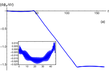
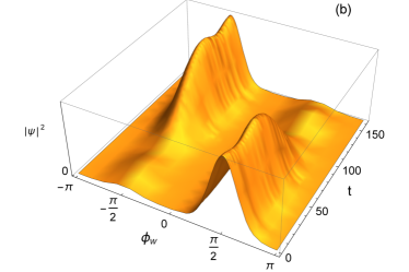
Figure 5: (Color online). Chirality switching with the Wannier state localized in the right well used as the initial state at $t=0$, under the action of a pulse with the amplitude $b=0.5\Delta$ and the duration of $\Delta t_{1}=2\pi/\omega_{B}$, followed by another pulse of the same amplitude after the time interval of $\Delta t_{2}=\pi\hbar/\Delta$. Shown are: (a) the average angular velocity $\langle d\phi_{w}/d\tau\rangle$ and (b) the probability density $|\psi|^{2}$ as functions of the dimensionless time $\tau=\hbar t/2m$ for $\xi=5$.

III.2 Quantum chirality dynamics

When the torque is much smaller than the barrier height, $b\ll U$, chirality dynamics can still be excited via quantum tunneling effects. The physics in this regime is similar to that of a current-biased Josephson junction (or, equivalently, a torque-driven quantum planar rotator, see the comprehensive review in [36]).

To analyze the quantum chirality dynamics, it is convenient to pass from the wave function $\Psi(\phi_{w})$ to a unitary-transformed one $\psi=e^{ik(t)\phi_{w}}\Psi$, with

$$\hbar k(t)=\int_{0}^{t}b(t^{\prime})dt^{\prime},$$ (33)

which brings the Hamiltonian to the explicitly periodic, time-dependent form (the so-called “periodic gauge”)

$$\tilde{\mathcal{H}}=\frac{\hbar^{2}}{2m}\left\{\left(-i\frac{\partial}{\partial\phi_{w}}-k(t)\right)^{2}+\frac{\xi^{2}}{4}\cos^{2}\phi_{w}\right\}.$$ (34)

In this gauge one can solve the time-dependent Schrödinger equation $i\hbar\partial_{t}\psi=\tilde{\mathcal{H}}\psi$ with periodic boundary conditions $\psi(\phi)=\psi(\phi+2\pi)$.

Consider first the case of a constant applied current, $\hbar k=bt$. If the energy gain on traversing between the wells is sufficiently small compared to the lowest level tunnel splitting, $\pi b\ll\Delta$, the single-band approximation can be used. The angular velocity $\langle d\phi_{w}/dt\rangle$ should exhibit Bloch oscillations around zero average value, with the frequency

$$\omega_{B}=\pi b/\hbar$$ (35)

and the amplitude $\bar{\omega}_{m}\simeq\pi\Delta/2\hbar$. The amplitude of the angle oscillations is thus $\phi_{\text{max}}\simeq\Delta/b$ and can be sufficiently large. For short times $t\ll 1/\omega_{B}$ the Bloch oscillation is indistinguishable from the accelerated rotation. Numerical solution of the time-dependent Schrödinger equation indeed shows such Bloch oscillations, albeit with an additional modulation with the frequency of about $\omega$ that corresponds to the transition between the ground state $\psi_{0}$ and the third excited state $\psi_{3}$, see Fig. 3. This happens due to the fact that the matrix element $\langle\psi_{3}|\hat{p}|\psi_{0}\rangle$ is large, allowing for an efficient excitation of $\psi_{3}$ mode. The amplitude of this additional modulation grows with increasing the current and gets more pronounced when the energy gain becomes comparable with the lowest level tunnel splitting.

In the regime of the energy gain $\pi b\gtrsim\Delta$ but still much smaller than the barrier height, the Wannier-Stark localization allows one to keep the wave function of the DW localized inside one of the wells, see Fig. 4(d). Applying two current pulses separated by one half of the Rabi period $\pi\hbar/\Delta$, one can flip the localized state from one well to the other, see Fig. 5. Note that such a switching does not suffer from inertial effects that occur when trying to kick the DW from one well to the other in the classical regime.

Thus, one can manipulate the chirality degree of freedom by the weak torque $\pi b\sim\Delta$, which corresponds to the operating current density

$$j^{q}=j^{cl}f(\xi),$$ (36)

considerably smaller than the classical switching threshold (32) for $\xi\gg 1$.

Such a quantum manipulation, however, can manifest itself only below certain “crossover” temperature $T_{c}$ which can be roughly estimated [22] by equating the quantum tunneling rate $\Delta$ and the thermal escape rate $\hbar\omega e^{-U/T}$. This estimate yields

$$T_{c}\sim U/\ln\left[4/\left(\xi f(\xi)\right)\right].$$ (37)

The speed of quantum chirality switching is obviously limited by the tunnel splitting, with the maximum “operating frequency” about $\Delta/\hbar$.

In the presence of a finite damping $\eta$, at very low bias $b/\hbar\eta<\bar{\omega}_{m}$ there is a steady rotation with the angular velocity $\bar{\omega}=b/\hbar\eta$, similar to the classical regime. When bias $b$ exceeds the threshold value $\hbar\eta\bar{\omega}_{m}\sim\eta\Delta$, the angular velocity starts Bloch oscillation, and its average (steady) value drops as $1/b$ [36].

Finally, for a strong bias the chirality dynamics can exhibit the Zener breakdown (interband tunneling) leading to an accelerated rotation, see Fig. 6; a finite damping would again change this to a steady rotation.

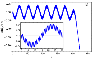
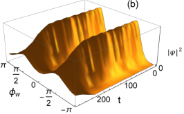
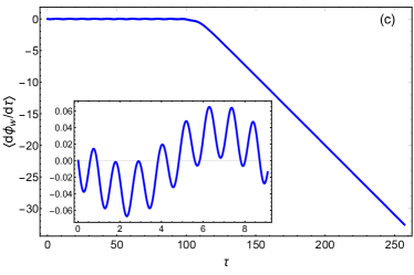
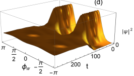
Figure 6: (Color online). Zener breakdown for a strong bias: (a), (c) the average angular velocity $\langle d\phi_{w}/d\tau\rangle$, and (b), (d) the probability density $|\psi|^{2}$ as functions of the dimensionless time $\tau=\hbar t/2m$ for $\xi=5$. The bias is $b=1.5\Delta$ in (a), (b), and $b=5\Delta$ in (c), (d) . The ground state for $b=0$ has been used as the initial state at $t=0$.

III.3 Estimates

III.3.1 Antiferromagnet or altermagnet

For an AF or AM, parameter $\xi$ takes the form

$$\xi=2N_{\perp}S\sqrt{\rho}$$ (38)

and thus depends only on the rhombicity parameter $\rho$ and not on the absolute values of material constants (exchange coupling $J$ and magnetic anisotropy $K$).

To achieve the quantum reduction of the switching threshold, while keeping the switching speed reasonably high, one has to work in the regime of moderate values of $\xi\sim 3-6$, thus the number of magnetic atoms in the cross-section of the DW cannot be much larger than $N_{\perp}\sim 100$. To keep $\xi$ moderate, the rhombicity has to be small (nearly uniaxial anisotropy), but it should not be too small as it would drive down the crossover temperature. To further increase $T_{c}$, it is favorable to increase the exchange and anisotropy constants $J$, $K$ (although that simultaneously increases $j^{q}$).

For instance, a DW in a nanowire with $3\times 3\;\text{nm}$ cross-section ($N_{\perp}\sim 100$ with $a\sim 3$ Å), with $J\sim 100\,\text{K}$, $K\sim 5\,\text{K}$, $S=1$, and $\rho\sim 10^{-3}$ will have the operating current density $j^{q}\sim 10^{3}\text{A/cm${}^{2}$}$ in the quantum regime below the crossover temperature $T_{c}\sim 0.75\text{K}$. Bloch oscillations excited by such a current will have the frequency of $\sim 4\,\text{GHz}$, the maximum switching frequency being roughly of the same value. Those Bloch oscillations, however, will be modulated by the frequency of about $\omega_{0}\sim 0.3\,\text{THz}$.

III.3.2 Ferromagnet

For a FM, parameter $\xi$

$$\xi=4N_{\perp}^{3/2}\frac{S}{a}\left(\frac{\rho E_{0}}{G}\right)^{1/2}$$ (39)

apparently scales as $N_{\perp}^{3/2}$, however in fact the scaling is linear if one takes into account that the pinning constant $G$ must also scale linearly with $N_{\perp}$. Following [22], one can model the pinning as caused by $N_{p}$ layers of impurities with an increased anisotropy constant $K^{\prime}>K$ and obtain the estimate $G\sim N_{p}N_{\perp}K^{\prime}/\delta^{2}$, which yields

$$\xi=4N_{\perp}S^{2}\left(\frac{\rho J}{N_{p}K^{\prime}}\right)^{1/2}\left(\frac{2J}{K}\right)^{1/4}.$$ (40)

It is easy to see that in FM $\xi$ is enhanced by the large factor $\frac{\delta}{a}\left(\frac{E_{0}}{N_{p}K^{\prime}}\right)^{1/2}$ compared to the AF case (38), and thus the tunnel splitting, which exponentially decreases with $\xi$, is much smaller in FM. Even for strong uniaxial anisotropy, the switching frequency can hardly be expected to reach more than a few MHz, and the tunneling will most likely be suppressed by damping.

IV Summary

We have studied different scenarios of manipulating the internal degree of freedom (chirality) of a pinned mesoscopic domain wall by means of applying external current, in several types of magnetic materials. While one needs spin-polarized current to control chirality in ferro- and antiferromagnets, we have shown that in the emerging novel class of magnetic materials known as altermagnets chirality can be manipulated by a regular, non-polarized charge current. Chirality oscillations (rotation of the domain wall) can be excited by current in ferro- as well as antiferromagnets, and the required current densities can be significantly reduced in magnetic materials with nearly uniaxial magnetic anisotropy. At very low temperatures, quantum tunneling effects open the possibility for controlling the chirality dynamics by current densities which can be an order of magnitude smaller than those required to excite it classically. Those very low currents can excite Bloch oscillations of the domain wall angular velocity with frequencies of the order of a few GHz, modulated by oscillations at much higher frequencies in the THz domain. Beside exciting the oscillations, in the quantum regime it is possible to perform a controlled switching between different chiral states, with inertial effects suppressed by the Wannier-Stark localization, albeit with the payoff of a limited switching speed.

In this paper, we have focused on the problem of manipulating the chirality by means of the applied current. There is another intriguing possibility, namely to read out the quantum state of the domain wall by measuring its conductance, which is left for the future work.

*

Appendix A Current coupling to the order parameter in ferro-, antiferro- and altermagnets

The goal of this Appendix is to give a derivation of the current coupling to the order parameter in altermagnets [12], but we would like to provide the necessary context by giving a brief overview of ferro- and antiferromagnetic cases first.

It is convenient to start from a tight-binding model for conduction electrons described by the Hamiltonian

$$H_{sd}=-t\sum_{\langle ll^{\prime}\rangle}(\psi_{l}^{\dagger}\psi_{l^{\prime}}^{\vphantom{\dagger}}+\text{h.c.})-J_{sd}\sum_{l}\psi_{l}^{\dagger}(\bm{\sigma}\cdot\bm{S}_{l})\psi_{l}^{\vphantom{\dagger}},$$ (41)

where $l$ numbers lattice sites, $\psi_{l}=(c^{\uparrow}_{l},c^{\downarrow}_{l})^{T}$ is the two-component spinor describing the conduction electrons (in the frame with the quantization axis $\bm{n}_{0}$), $t$ is the hopping amplitude between nearest neighbor site pairs $\langle ll^{\prime}\rangle$, and $J_{sd}$ is the exchange coupling to localized spins $\bm{S_{l}}$ which are treated as classical vectors. The Lagrangian corresponding to this tight-binding model can be written as

$$L_{sd}=i\frac{\hbar}{2}\sum_{l}\left(\psi_{l}^{\dagger}\partial_{t}\psi_{l}^{\vphantom{\dagger}}-\partial_{t}\psi_{l}^{\dagger}\psi_{l}^{\vphantom{\dagger}}\right)-H_{sd}.$$ (42)

Ferromagnet.–

In a ferromagnet, $\bm{S_{l}}=S\bm{n}_{l}$, where the unit vector $\bm{n}$ can be assumed to vary smoothly across the lattice. Performing local unitary transformation $\psi_{l}=U(\bm{n})\chi_{l}$ with

$$U(\bm{n}_{l})=\bm{\sigma}_{l}\cdot\bm{e}_{l},\quad\bm{e}=\frac{\bm{n}_{0}+\bm{n}}{[2(1+\bm{n}\cdot\bm{n}_{0})]^{1/2}},$$ (43)

we rotate the quantization lattice at each lattice site to $\bm{n}_{l}$, so that the interaction term $\psi_{l}^{\dagger}(\bm{\sigma}\cdot\bm{S}_{l})\psi_{l}=S\chi_{l}^{\dagger}\sigma_{z}\chi_{l}$ is diagonalized in this twisted frame. This twist modifies hopping as follows:

$$\psi_{l}^{\dagger}\psi_{l^{\prime}}=(\bm{e}_{l}\cdot\bm{e}_{l^{\prime}})\chi_{l}^{\dagger}\chi_{l^{\prime}}+i(\bm{e}_{l}\cdot\bm{e}_{l^{\prime}})\cdot(\chi_{l}^{\dagger}\bm{\sigma}\chi_{l^{\prime}}).$$ (44)

One can pass to the continuum description, by setting $l\mapsto\bm{r}$, $l^{\prime}\mapsto\bm{r}+\bm{a}$, and perform the gradient expansion. Up to the second order in gradients, the hopping term in (41) takes the form

$$ta^{2}(\nabla_{a}\psi^{\dagger})(\nabla_{a}\psi)=ta^{2}\big{(}\nabla\chi^{\dagger}-i\chi^{\dagger}\mathsf{A}_{a}\big{)}\big{(}\nabla\chi+i\mathsf{A}_{a}\chi\big{)},$$ (45)

where the matrix gauge field $\mathsf{A}_{a}=(\bm{\mathcal{A}}_{a}\cdot\bm{\sigma})$ is defined via the set of vector gauge fields

$$\bm{\mathcal{A}}_{a}=(\bm{e}\times\nabla_{a}\bm{e})=\frac{(\bm{n}_{0}+\bm{n})\times\nabla_{a}\bm{n}}{2(1+\bm{n}\cdot\bm{n}_{0})},$$ (46)

and we have used the shorthand notation $\nabla_{a}\equiv\frac{1}{a}(\bm{a}\cdot\bm{\nabla})$.

The expression (45) describes the kinetic energy of electrons with the effective mass

$$m_{*}=\hbar^{2}/(2ta^{2})$$ (47)

coupled to SU(2) gauge field $\mathsf{A}$. In Eq. (45), the term quadratic in $\mathsf{A}$ can be recast as $ta^{2}(\chi^{\dagger}\chi)(\nabla\bm{e})^{2}$ and leads to a renormalization of the FM exchange energy in the presence of a finite density of conduction electrons, so we will omit it in what follows. The term linear in $\mathsf{A}$ yields the following contribution to the Lagrangian density in the continuum approximation:

$$-2\bm{j}^{(s)}_{a}\cdot\bm{\mathcal{A}}_{a},$$ (48)

where

$$\bm{j}^{(s)}_{a}=-\frac{i\hbar^{2}}{4m_{*}V_{0}}\big{(}\chi^{\dagger}\bm{\sigma}\nabla_{a}\chi-\nabla_{a}\chi^{\dagger}\bm{\sigma}\chi\big{)}$$ (49)

is the spin current density in the $\bm{a}$ direction (the components of the vector $\bm{j}^{(s)}_{a}$ are taken in the rotated frame), and $V_{0}$ is the volume of the magnetic unit cell.

The first term in the Lagrangian (42), after performing the unitary twist, similarly yields another contribution to the Lagrangian density

$$-2\bm{\tau}^{(s)}\cdot\bm{\mathcal{A}}_{0},$$ (50)

where the gauge field $\bm{\mathcal{A}}_{0}$ has the form (46) with the replacement $\nabla_{a}\mapsto\partial_{t}$, and $\bm{\tau}^{(s)}$ is the spin density of the conduction electrons in the locally rotated frame (i.e., with respect to the order parameter):

$$\bm{\tau}^{(s)}=\frac{\hbar}{2V_{0}}\left(\chi^{\dagger}\bm{\sigma}\chi\right).$$ (51)

Integrating (48) and (50) over the volume of the nanowire, one gets the expression (8).

Antiferromagnet.–

In a two-sublattice antiferromagnet, $\bm{S_{l}}=S(\bm{m}_{l}+\eta_{l}\bm{n}_{l})$, where $\eta_{l}$ takes alternating values $\pm 1$ on two sublattices, and $\bm{m}$ and $\bm{n}$ correspond to the magnetization and the Néel vector, respectively, satisfying the constraints $\bm{m}\cdot\bm{n}=0$ and $\bm{m}^{2}+\bm{n}^{2}=1$. For smooth spin textures, the magnetization $\bm{m}$ can be viewed as a “slave field” which is proportional to space and time gradients of the order parameter $\bm{n}$, so typically $|\bm{m}|\ll|\bm{n}|$, and one can for our purposes neglect $\bm{m}$ and view $\bm{n}$ as a unit vector. Performing the same unitary transformation (43) adjusts the electron quantization axes to the local Néel vector direction and brings the interaction term to its form for the homogeneous AF texture. The hopping term produces [32] the gauge-field coupling (48), while the dynamic term in the Lagrangian produces [24] the gauge-field couplings (50), similar to the FM case. We remark that our derivation here is kept simplified for the sake of clarity. The more rigorous derivation [33, 24] leads to the additional overall factor $(1-\zeta^{2})$ in front of both (48) and (50), with $\zeta\propto t/J_{sd}$. Here we assume that $\zeta\ll 1$ and neglect this additional factor. It should be remarked that non-adiabatic contributions to spin transfer torque in an antiferromagnet have been shown [37] to lead to the coupling of same form (48), albeit multiplied by a non-universal factor.

Altermagnet.–

As a starting point, we take one of the minimal toy models of an altermagnet [12], described by the Hamiltonian (25) and Fig. 2. In each unit cell we introduce the magnetization $\bm{m}$ and the Néel vector $\bm{n}$:

$$\bm{S}_{1,l}=S(\bm{m}_{l}+\bm{n}_{l}),\quad\bm{S}_{2,l}=S(\bm{m}_{l}-\bm{n}_{l}).$$ (52)

In what follows, we assume that in the homogeneous unperturbed state $\bm{m}=0$, and $\bm{l}=\bm{n}_{0}$, and $\bm{n}_{0}$ is also the quantization axis for electron spinors $\psi_{l}$.

We again perform unitary transformation (43) to rotate the electron quantization axes to the local Néel vector direction $\bm{n}_{l}$. The spin-independent term in the hopping will again acquire the gauge-field modification (45), leading to the contribution of the form (48) coupling texture gradients to the spin current. However, it is easy to show that the spin-dependent hopping leads to another contribution which couples not to the spin current, but to the charge current. Indeed, the $t^{\prime}$-term transforms as follows: $\psi_{l}^{\dagger}(\bm{\sigma}\cdot\bm{S}_{ll^{\prime}})\psi_{l^{\prime}}=\chi_{l}^{\dagger}W_{ll^{\prime}}\chi_{l^{\prime}}$, where

$$W_{ll^{\prime}} = -i\bm{S}_{ll^{\prime}}\cdot(\bm{e}_{l}\times\bm{e}_{l^{\prime}})\;\mathds{1}$$

$$+ \Big{\{}\bm{e}_{l}(\bm{e}_{l^{\prime}}\cdot\bm{S}_{ll^{\prime}})+\bm{e}_{l^{\prime}}(\bm{e}_{l}\cdot\bm{S}_{ll^{\prime}})-\bm{S}_{ll^{\prime}}\cdot(\bm{e}_{l}\cdot\bm{e}_{l^{\prime}})\Big{\}}\cdot\bm{\sigma}.$$

Passing to the continuum description, $l\mapsto\bm{r}$, $l^{\prime}\mapsto\bm{r}+\bm{a}$, and performing the gradient expansion, one can see that up to the first order in gradients $W$ takes the following form:

$$W = \eta_{\bm{a}}(\bm{n}_{0}\cdot\bm{\sigma})+\Big{(}2\bm{e}(\bm{e}\cdot\bm{m})-\bm{m}\Big{)}\cdot\bm{\sigma}$$

$$+ \eta_{\bm{a}}a\Big{(}\bm{e}(\bm{n}\cdot\nabla_{a}\bm{e})+\nabla_{a}\bm{e}(\bm{n}\cdot\bm{e})\Big{)}\cdot\bm{\sigma}$$

$$- ia\bm{n}\cdot\big{(}\bm{e}\times\nabla_{a}\bm{e})\mathds{1},$$

where $\eta_{\bm{a}}=\pm 1$ for $\bm{a}=\hat{\bm{x}}$, and $\bm{a}=\hat{\bm{y}}$, respectively. Similar to the low-energy description of antiferromagnets, the magnetization $\bm{m}$ is linear in gradients of the order parameter $\bm{n}$. The gradient-free term in $W$ corresponds to the spin-dependent hopping in the homogeneous AF order.

In the first order in gradients, there are two contributions to $W$. One of them is a superposition of Pauli’s matrices, and describes coupling of the electron spin density to the gradient of the order parameter; in what follows, we will not be interested in that contribution as it does not involve currents. The other term in $W$, which is purely imaginary and proportional to the unit matrix, leads to the following contribution to the Lagrangian density in the continuum approximation:

$$-\frac{t^{\prime}}{t}\frac{\hbar}{e}\sum_{\bm{a}=\hat{\bm{x}},\hat{\bm{y}}}j^{(c)}_{a}\eta_{\bm{a}}(\bm{n}\cdot\bm{\mathcal{A}}_{a}),$$ (55)

where

$$j^{(c)}_{a}=-\frac{ie\hbar}{2m_{*}V_{0}}\big{(}\chi^{\dagger}\nabla_{a}\chi-\nabla_{a}\chi^{\dagger}\chi\big{)}$$ (56)

is the density of the charge current in the direction $\bm{a}$. Thus, in an altermagnet the Néel vector gradient couples to the usual electric current, in contrast to the FM or AF case, where coupling is only to the spin-polarized current. Taking into account (46), the coupling (55) can be recast as

$$-\kappa\frac{\hbar}{2e}\sum_{\bm{a}=\hat{\bm{x}},\hat{\bm{y}}}j^{(c)}_{a}\eta_{\bm{a}}\bm{A}(\bm{n}_{0},n)\cdot\nabla_{a}\bm{n},$$ (57)

where the Dirac monopole vector potential $\bm{A}(\bm{n}_{0},n)$ is defined in (3), and $\kappa=t^{\prime}/t$ is the relative strength of the spin-dependent hopping.

Finally, the contribution from the dynamic part of the Lagrangian (42) will result in the same coupling term (50). If the current is not spin-polarized, this contribution vanishes, and the only surviving contribution is (57).

References

- Manchon et al. [2019] A. Manchon, J. Železný, I. M. Miron, T. Jungwirth, J. Sinova, A. Thiaville, K. Garello, and P. Gambardella, Current-induced spin-orbit torques in ferromagnetic and antiferromagnetic systems, Rev. Mod. Phys. 91, 035004 (2019).
- Jungwirth et al. [2016] T. Jungwirth, X. Marti, P. Wadley, and J. Wunderlich, Antiferromagnetic spintronics, Nat. Nanotechnol. 11, 231 (2016).
- Nagaosa et al. [2010] N. Nagaosa, J. Sinova, S. Onoda, A. H. MacDonald, and N. P. Ong, Anomalous Hall effect, Reviews of Modern Physics 82, 1539 (2010), arXiv:0904.4154 .
- Gomonay and Loktev [2014] E. V. Gomonay and V. M. Loktev, Spintronics of antiferromagnetic systems (Review Article), Low Temperature Physics 40, 17 (2014).
- Gomonay et al. [2016] O. Gomonay, T. Jungwirth, and J. Sinova, High Antiferromagnetic Domain Wall Velocity Induced by Néel Spin-Orbit Torques, Physical Review Letters 117, 017202 (2016).
- Gomonay et al. [2017] O. Gomonay, T. Jungwirth, and J. Sinova, Concepts of antiferromagnetic spintronics, Physica Status Solidi - Rapid Research Letters 11, 1700022 (2017), arXiv:1701.06556 .
- Baltz et al. [2018] V. Baltz, A. Manchon, M. Tsoi, T. Moriyama, T. Ono, and Y. Tserkovnyak, Antiferromagnetic spintronics, Rev. Mod. Phys. 90, 015005 (2018).
- Chen et al. [2022] H. Chen, P. Qin, H. Yan, Z. Feng, X. Zhou, X. Wang, Z. Meng, L. Liu, and Z. Liu, Noncollinear antiferromagnetic spintronics, Materials Lab 1, 220032 (2022).
- Železný et al. [2014] J. Železný, H. Gao, K. Výborný, J. Zemen, J. Mašek, A. Manchon, J. Wunderlich, J. Sinova, and T. Jungwirth, Relativistic Néel-Order Fields Induced by Electrical Current in Antiferromagnets, Physical Review Letters 113, 157201 (2014), arXiv:1410.8296 .
- Wadley et al. [2016] P. Wadley, B. Howells, J. Železný, C. Andrews, V. Hills, R. P. Campion, V. Novák, K. Olejník, F. Maccherozzi, S. S. Dhesi, S. Y. Martin, T. Wagner, J. Wunderlich, F. Freimuth, Y. Mokrousov, J. Kuneš, J. S. Chauhan, M. J. Grzybowski, A. W. Rushforth, K. Edmond, B. L. Gallagher, and T. Jungwirth, Electrical switching of an antiferromagnet, Science 351, 587 (2016), arXiv:1503.03765 .
- Bodnar et al. [2018] S. Y. Bodnar, L. Šmejkal, I. Turek, T. Jungwirth, O. Gomonay, J. Sinova, A. A. Sapozhnik, H. J. Elmers, M. Klaüi, and M. Jourdan, Writing and reading antiferromagnetic Mn2Au by Neél spin-orbit torques and large anisotropic magnetoresistance, Nature Communications 9, 1 (2018).
- Šmejkal et al. [2022a] L. Šmejkal, J. Sinova, and T. Jungwirth, Emerging research landscape of altermagnetism, Phys. Rev. X 12, 040501 (2022a).
- Šmejkal et al. [2020] L. Šmejkal, R. González-Hernández, T. Jungwirth, and J. Sinova, Crystal time-reversal symmetry breaking and spontaneous Hall effect in collinear antiferromagnets, Science Advances 6, eaaz8809 (2020), arXiv:1901.00445 .
- Feng et al. [2022] Z. Feng, X. Zhou, L. Šmejkal, L. Wu, Z. Zhu, H. Guo, R. González-Hernández, X. Wang, H. Yan, P. Qin, X. Zhang, H. Wu, H. Chen, Z. Meng, L. Liu, Z. Xia, J. Sinova, T. Jungwirth, and Z. Liu, An anomalous Hall effect in altermagnetic ruthenium dioxide, Nature Electronics 5, 735–743 (2022).
- Šmejkal et al. [2022b] L. Šmejkal, A. B. Hellenes, R. González-Hernández, J. Sinova, and T. Jungwirth, Giant and tunneling magnetoresistance in unconventional collinear antiferromagnets with nonrelativistic spin-momentum coupling, Phys. Rev. X 12, 011028 (2022b).
- Chudnovsky and Tejada [2005] E. M. Chudnovsky and J. Tejada, Macroscopic Quantum Tunneling of the Magnetic Moment, Cambridge Studies in Magnetism, Vol. 4 (Cambridge University Press, 2005).
- Gatteschi et al. [2006] D. Gatteschi, R. Sessoli, and J. Villain, Molecular Nanomagnets (Oxford University Press, 2006).
- Ivanov [2005] B. A. Ivanov, Mesoscopic antiferromagnets: statics, dynamics, and quantum tunneling (review), Low Temp. Physics 31, 635 (2005).
- Ivanov and Kolezhuk [1994] B. A. Ivanov and A. K. Kolezhuk, Quantum tunneling of magnetization in a small-area domain wall, JETP Letters 60, 805 (1994).
- Ivanov and Kolezhuk [1995] B. A. Ivanov and A. K. Kolezhuk, Quantum tunneling and quantum coherence in a topological soliton of quasi-one-dimensional antiferromagnet, Low Temp. Phys. 21, 760 (1995).
- Braun and Loss [1996] H.-B. Braun and D. Loss, Berry’s phase and quantum dynamics of ferromagnetic solitons, Phys. Rev. B 53, 3237 (1996).
- Takagi and Tatara [1996] S. Takagi and G. Tatara, Macroscopic quantum coherence of chirality of a domain wall in ferromagnets, Phys. Rev. B 54, 9920 (1996).
- Ivanov et al. [1998] B. A. Ivanov, A. K. Kolezhuk, and V. E. Kireev, Chirality tunneling in mesoscopic antiferromagnetic domain walls, Phys. Rev. B 58, 11514 (1998).
- Cheng and Niu [2014] R. Cheng and Q. Niu, Dynamics of antiferromagnets driven by spin current, Phys. Rev. B 89, 081105 (2014).
- Ovcharov et al. [2022] R. Ovcharov, E. Galkina, B. Ivanov, and R. Khymyn, Spin Hall Nano-Oscillator Based on an Antiferromagnetic Domain Wall, Phys. Rev. Appl. 18, 024047 (2022).
- Auerbach [1994] A. Auerbach, Interacting Electrons and Quantum Magnetism (Springer-Verlag, 1994).
- Schryer and Walker [2003] N. L. Schryer and L. R. Walker, The motion of 180° domain walls in uniform dc magnetic fields, Journal of Applied Physics 45, 5406 (2003), https://pubs.aip.org/aip/jap/article-pdf/45/12/5406/7951916/5406_1_online.pdf .
- Shraiman and Siggia [1988] B. I. Shraiman and E. D. Siggia, Mobile Vacancies in a Quantum Heisenberg Antiferromagnet, Phys. Rev. Lett. 61, 467 (1988).
- Bazaliy et al. [1998] Y. B. Bazaliy, B. A. Jones, and S.-C. Zhang, Modification of the Landau-Lifshitz equation in the presence of a spin-polarized current in colossal- and giant-magnetoresistive materials, Phys. Rev. B 57, R3213 (1998).
- Kohno and Shibata [2007] H. Kohno and J. Shibata, Gauge field formulation of adiabatic spin torques, Journal of the Physical Society of Japan 76, 063710 (2007).
- Galkina et al. [2008] E. G. Galkina, B. A. Ivanov, S. Savel’ev, and F. Nori, Chirality tunneling and quantum dynamics for domain walls in mesoscopic ferromagnets, Phys. Rev. B 77, 134425 (2008).
- Swaving and Duine [2011] A. C. Swaving and R. A. Duine, Current-induced torques in continuous antiferromagnetic textures, Phys. Rev. B 83, 054428 (2011).
- Cheng and Niu [2012] R. Cheng and Q. Niu, Electron dynamics in slowly varying antiferromagnetic texture, Phys. Rev. B 86, 245118 (2012).
- Sasaki [1982] K. Sasaki, Finite-Temperature Corrections to Kink Free Energies, Progress of Theoretical Physics 68, 411 (1982), https://academic.oup.com/ptp/article-pdf/68/2/411/5454416/68-2-411.pdf .
- Cheng et al. [2016] R. Cheng, D. Xiao, and A. Brataas, Terahertz Antiferromagnetic Spin Hall Nano-Oscillator, Phys. Rev. Lett. 116, 207603 (2016).
- Sonin [2022] E. B. Sonin, Quantum rotator and Josephson junction: compact vs. extended phase and dissipative quantum phase transition (2022), arXiv:2201.04998 [cond-mat.other] .
- Fujimoto [2021] J. Fujimoto, Adiabatic and nonadiabatic spin-transfer torques in antiferromagnets, Phys. Rev. B 103, 014436 (2021).