Dynamics of unsteady premixed flames in meso scale channels under varying wall heating conditions

Abstract

Understanding the dynamics of flames at small scales opens up opportunities to enhance the performance of small-scale power generation devices (which have potential appliances in micro-electro-mechanical systems), micro-reactors (which are extensively used in the field of quantitative chemistry), fire safety devices, and numerous other systems that confine combustion to micro/meso scales. The current study delves into the dynamics of laminar premixed methane-air flames in mesoscale channels subjected to an axial bimodal wall temperature profile (established using two external heaters). The work involves varying the axial distance between the temperature peaks of the bimodal profile and investigating flame dynamics across a wide range of equivalence ratios ($\Phi$) and Reynolds numbers (Re). The dynamics are also compared against a baseline configuration that utilizes a single heater to establish an axial unimodal wall temperature profile. Apart from the already documented observations of stationary stable flames and unsteady flames with repetitive extinction and ignition (FREI) characteristics, this study identifies an additional unsteady propagating flame (PF). The dynamics of the latter-mentioned unsteady flames are the focus of the current study. FREI regime flames, upon auto-ignition, propagate upstream and extinguish after a characteristic travel distance. They repeat periodically with a frequency that is found to increase with $Re$ and $\Phi$. At characteristic separation distances between the bimodal temperature peaks, in a narrow range of $Re$ and $\Phi$, the FREI dynamics alter and are found to exhibit additional peaks in their OH chemiluminescence and flame speed signatures. They are identified as a sub-regime in FREI and are termed ’Diverging FREI’. While FREI appeared at stoichiometric and fuel-rich conditions, propagating flames were observed at the equivalence ratio of $0.8$. Unlike the FREI regime, propagating flames continue to travel till they reach the upstream end of the combustor tube (where they extinguish upon encountering a meshed constriction). These flames are associated with a characteristic heat-release-rate oscillation that couples with the pressure fluctuations. The frequency of these coupled oscillations is close to the natural harmonic of the combustor tube. The dynamics of FREI and PF are discussed in detail with arguments that justify the trends observed with respect to the Reynolds number, equivalence ratio, and wall temperature profiles. A simple theoretical model is also presented that accounts for the observed thermo-acoustic coupling in propagating flames.

Novelty and Significance Statement

The work investigates the dynamics of premixed methane-air flames in mesoscale channels subjected to axial bimodal wall heating profiles. Alongside the well-documented unsteady mesoscale flame regime of FREI (flames with repetitive extinction and ignition), an additional unsteady propagating flame regime is identified that travels throughout the length of the combustor tube without extinction. Propagating flames (PF) exhibit a characteristic acoustic fluctuation that couples with the heat release rate fluctuations at frequencies close to the natural harmonic of the combustor tube. Interesting flame bifurcation behaviors are observed in these unsteady flames (FREI and PF) in a characteristic range of Reynolds number and equivalence ratios when the axial separation distance between the bimodal heating peaks is varied. Understanding the dynamics of such meso-channel flame regimes can open up potential opportunities to enhance the performance of micro-reactors and micro power generators.

Author Contributions

Akhil Aravind: Conceptualisation, Experiments, Data Analysis, Writing - Original Draft. Gautham Vadlamudi: Conceptualisation, Experiments, Writing - Review & Editing. Saptarshi Basu: Conceptualisation, Data Analysis, Writing - Review & Editing, Fund acquisition.

Nomenclature

• Reynolds Number

• Stationary Flames

• Strouhal Number

• Seperation distance between the primary and secondary heaters

• Threshold Intensity

• Flame propagation speed

• Inner diameter of the quartz combustor tube

• Time period of repetition of an unsteady flame

• Convective time scale associated with the flow

• Mean flow temperature

• Inner radius of the combustor tube

• Outer radius of the combustor tube

• time

• thermal diffusivity

• Temperature at the outer wall of the quartz tube

• Temperature at the inner wall of the quartz tube

• Heat flux at the inner wall of the quartz tube

• Length of the quartz combustor tube

• Nusselt number

• Mean flow velocity of premixed gases inside the quartz tube

• Time between ignition and OH chemiluminescence peak

• Time between OH chemiluminescence peak and flame extinction

• Time between flame extinction and re-ignition

• Time between the first and first and second peaks in a D-FREI

• Frequency of repetition of unsteady flames

• Maximum flame propagation speed in a flame cycle

• Reactant mass consumption rate

• Unburnt gas mixture density

• Cross sectional area of the combustor tube

• Reaction rate

• Activation Energy

• Burnt gas temperature

• Flame temperature

• Unburnt gas temperature

• Specific formation enthalpy of species $k$ at standard conditions

• Specific heat capacity of species $k$ at temperature $T$

• Heat losses

• Pre-heat zone thickness

• Flame travel(propagation) distance between ignition and extinction

• Axial distance along the combustor axis with the upstream end anchored as $x=0$

• Acoustic velocity in the unburnt gases

• Acoustic velocity in the burnt gases

• Position of the flame along the combustor axis with respect to the upstream end

• Heat release rate fluctuation

• Ratio of the specific heats at constant pressure and constant volume

• Wave number

1 Introduction

Rapid advances in micro-fabrication techniques have aided the miniaturization and integration of electro-mechanical systems on tiny chips. These micro-electro-mechanical systems (MEMS) find applications in areas ranging from biomedical devices to micro space/aerial vehicles. Currently, these devices rely on low-energy density batteries for their power requirements, which limits their portability and functionality. Micro/Meso combustors were initially conceived as potential alternatives to power these devices since the energy density of a typical liquid hydrocarbon is two orders higher in magnitude than standard alkaline/Li-ion batteries [1, 2, 3]. However, micro/meso scale combustion has found its way into other domains in the form of micro-reactors (that find extensive applications in quantitative chemistry [4]) and fire safety systems. In this context, ’micro’ describes combustors with a characteristic length scale smaller than the quenching diameter, while ’meso’ combustors have a larger length scale that is of the order of the quenching diameter [5].

When the size of the combustor decreases to micro or meso scales, the ratio of surface area to volume increases significantly. Consequently, wall heat losses become significant, rendering the flame vulnerable to both thermal and radical quenching. To maintain flames at such scales, a commonly employed approach involves recirculating the product gases upstream of the reaction zone. This process preheats the reactants and modifies the temperature gradient at the wall to reduce heat losses, thus sustaining the flames in channels smaller than the classical quenching limit [6]. In contrast to larger-scale combustors, where the combustor walls primarily serve as a sink for heat and radicals, the flame-wall interactions are more intricate at smaller scales. These interactions can, in fact, be such that the wall adds energy to the fluid, depending on the associated Biot and Fourier numbers. Such flame-wall coupling can thus introduce additional flame regimes which are otherwise not observed at large scales. The thermal properties of the walls, particularly thermal conductivity, are observed to exert a substantial impact on the temperature distribution along the wall and the overall behavior of the flame [7]. Furthermore, it has been observed that in small-scale combustors, elevated wall temperatures render the flame vulnerable to radical quenching [8, 9, 7], potentially influencing the overall flame dynamics. The ensuing discussion delves into commonly observed flame behaviors at small scales.

Maruta et al. [10, 11] conducted studies with a cylindrical quartz tube of inner diameter 2mm that acts as an optically accessible micro combustor for premixed methane-air flames. The effect of product gas re-circulation was imposed using two heating plates at the top and bottom of the tube. In addition to the stationary flames that establish themselves at a specific section within the channel, various unsteady flame behaviors were also documented. These included a flame exhibiting a series of ignition, propagation, extinction, and re-ignition events, referred to as FREI (Flames with Repetitive Extinction and Ignition), as well as a pulsating flame and a flame displaying traits of both pulsation and FREI. Similar observations were reported by Fan et al. [12] in methane-air premixed flames inside rectangular quartz channels of different characteristic length scales, all of which were of the order of the quenching diameter. Likewise, Richecoeur et al. [13] observed flame oscillations in curved mesoscale channels in fuel-rich conditions. Ju and Xu [14] conducted both theoretical and experimental studies on the propagation and extinction of flames at mesoscales. They found that a flame within a mesoscale channel could propagate at velocities exceeding that of an adiabatic flame, contingent upon the thermal characteristics and heat capacity of the channel walls. Furthermore, it is to be noted that, alongside product gas re-circulation, stream-wise heat conduction along the wall from the flame was also found to affect the reactant temperature upstream of the flame front [15], the extent of which was again subject to the thermal properties of the wall.

Jackson et al. [16] compared the problem of flame propagation/stabilization in narrow ducts to that of an edge flame and proposed a model that captured the transition between steady and unsteady flame solutions. The model only had thermal considerations and ignored hydrodynamic contribution by directly imposing a poiseuille velocity profile inside the duct. This treatment was further emphasized by Bieri et al. [17] and veeraragavan et al.[7]. Nonetheless, it was observed that the frequency of flame oscillations in unsteady flames aligned with the Strouhal number associated with the instability of the jet emerging from the micro/meso channels (St $\sim$ 0.4) [13], emphasizing the role of hydrodynamics in dictating the quantitative flame dynamics.

The Flame-wall interaction in unsteady flame regimes was extensively studied by Evans and Kyritsis [7, 18]. Their work showed that a thin wall serves a dual purpose: acting as a heat sink following ignition, resulting in flame extinction due to rapid heat losses, as well as enabling re-ignition since the wall temperature rises before extinction due to the associated low thermal inertia. Consequently, this leads to high-frequency extinction and re-ignition events (FREI) and can result in acoustic emissions. Acoustic phenomena were typically observed at the lowest possible equivalence ratio that sustained oscillatory flames and occurred very close to the extinction phenomena. Similar observations of sound emission with unsteady flames were reported by various other research groups [7, 18, 11, 10, 12, 13]. Nicoud et al. [19] attributed the sound generation to the contraction/expansion that happens during the extinction/re-ignition events associated with unsteady flames. The significance of such thermal effects was further emphasized by experimental results indicating that sound generation, or its absence, hinges primarily on the choice of wall material [7, 18]. The greater the thermal conductivity of the wall material, the more pronounced the sound emission becomes. Tse et al. [20] emphasized that this phenomenon is contingent on the specific apparatus used, and identified its origin as homogeneous explosions occurring at the tube entrance during the re-ignition process. Nevertheless, the exact cause of these acoustic phenomena associated with unsteady flames remains inconclusive.

Studies have also explored the micro/meso channel flame dynamics under different wall temperature profiles (all the investigated temperature profiles are monotonic along the combustor axis). Kang et al. [21] numerically investigated the dynamics of methane-air flames in microchannels under different wall temperature conditions and concluded that the flame propagation speed was not only dependent on the chemical heat release rate but also on the flame-wall heat exchange rate. Consequently, these factors collectively led to quantitative changes in the characteristics of the flame regimes at different wall temperature profiles. A similar study by Ratnakishore et al. [22] demonstrated the movement of ignition location to low wall temperature zones as the imposed axial wall temperature gradients were reduced.

Following up on the studies mentioned above, in this work, we investigate the dynamics of flames within mesoscale channels subjected to a bimodal wall heating pattern. This scenario holds practical significance in mesoscale rectangular Swiss-roll burners, where hot product gases follow a rectangular outward spiral path surrounding the inward rectangular spiral path for the reactants to reach the reaction-stabilized center of the combustor. The wall temperature is expected to decay monotonically as we move radially outward away from the reaction zone. However, as the flow decelerates at the corners of these rectangular spiral paths, regions with spikes in the wall temperature profile are formed. The existing literature provides compelling evidence suggesting that such spikes in the wall temperature profile have the potential to significantly influence flame-wall interactions, thereby inducing both quantitative and qualitative changes in the flame dynamics. The primary objective of our research is to thoroughly investigate this phenomenon and gain a deeper understanding of the associated flame dynamics. As our first step, we explore the behavior of unsteady premixed flames in channels that feature a bimodal wall heating profile. The bimodal profile is a simplified 1-D representation of the local temperature spike imposed over a monotonically decaying temperature profile (along the 1-D combustor axis in the upstream direction, away from the flame location), similar to that observed around the corners of a rectangular Swiss roll combustor.

2 Experimental Setup

2.1 Mesoscale combustor channel and external wall heating

A circular quartz channel of $5mm$ inner diameter ($d_{i}$) and $7mm$ outer diameter ($d_{o}$) is used as an optically accessible mesoscale combustor tube (Length: $380mm$). The effect of product gas upstream re-circulation is imposed using two external heaters: a dual torch (primary heater) and a flat flame burner (secondary heater), as depicted in Fig.1(a). The primary and secondary heaters, in combination, impose a bimodal wall heating profile. In the heating zones (tube sections directly above the primary and secondary heaters), the wall temperature profile shows a steep rise and fall in temperatures, peaking around $~{}1130K$ in the primary heating zone and around $~{}1025K$ in the secondary heating zone. The span over which the peak is maintained in the primary heating zone is very narrow compared to that imposed in the secondary heating zone (Fig.1(b)). The distance between the centers of the heaters, characterized by $d$, is varied to obtain different wall heating profiles. A $1mm$ K-type thermocouple was employed to measure the temperature along the inner walls of the combustor tube. It is to be noted that since the combustor tube is heated from below, the inner wall temperature is not uniform across the tubular cross section. Since the lower periphery of the inner wall is closer to the heaters, it is expected to have a higher wall temperature than the upper periphery. This difference was highest in the primary heating zone and was close to $2\%$. The plot in Fig.1(b) corresponds to the inner wall temperature measured along the lower periphery in the axial direction. The profiles are estimated from three sets of experimental measurements.

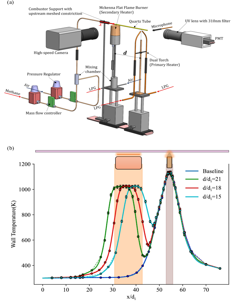
Figure 1: (a)Experimental Setup (b)Inner wall temperature profiles at different separation distances, $d/d_{i}$. The regions highlighted in purple and red represent the primary and secondary heating zones, respectively, for $d/d_{i}=18$. The solid lines in the plot correspond to profiles generated using a smoothening spline generated based on the data points.

Methane and air regulated through two precise mass flow controllers (Bronkhorst Flexi-Flow Compact with the range of 0-1.6 SLPM for $CH_{4}$ and 0-2 SLPM for air) are directed into a mixing chamber, where the streams mix into each other to create a homogeneous mixture, which is then subsequently fed into the quartz combustor tube at $x=0mm$ (upstream end). The flow rates of LPG (liquefied petroleum gas) and air into the heaters (primary and secondary) were controlled using precise pressure regulators and mass flow controllers (Alicat Scientific MCR-500SLPM), respectively.

In the discussions that follow, the $x$-axis is oriented along the combustor axis, extending in the downstream direction. The origin is set at $x=0mm$, marking the upstream end. The quartz tube connects to the upstream mixing chamber (via a flashback arrestor) at this section via a $1.5mm$ tubular constriction that houses a thin region of $100\mu m$ wire mesh just upstream of $x=0mm$.

It is to be noted that the initial $65mm$ segment of the quartz tube was inaccessible for imaging due to the presence of a steel support that held the $380mm$-long quartz combustor tube in the form of a cantilever.

2.2 High-speed flame imaging and data acquisition from PMT and Microphone

A Phantom Miro coupled with a 100mm Tokina macro-lens was used for high-speed flame imaging. The dynamics were captured at 4000 frames per second ($250\mu s$ exposure time) with a frame size of 1280 x 120 pixels (resolution of $200\mu$m per pixel). The data was used to track the position of the flame. The flame’s OH chemiluminescence signal was captured using a Hamamatsu photomultiplier tube (H11526-110-NF), and the pressure field fluctuation was recorded using a microphone (PCB 130E20). The data from the Photomultiplier tube (PMT) and the microphone was acquired using an NI-DAQ (PCI 6251) at 12000 Hz.

The flame images from the high-speed camera were processed in ImageJ, where they were subjected to thresholding using the Otsu thresholding technique, an integral feature of ImageJ. Otsu’s thresholding algorithm calculates a single intensity threshold value (denoted as $I_{f}$) that separates all the pixels within an image into two categories: foreground and background. This threshold value $(I_{f})$ is determined by minimizing the variance in intensity within each class or, conversely, maximizing the variance between the two classes. The flame’s outline is then isolated based on this threshold intensity $(I_{f})$. Pixels $(i,j)$ with intensities greater than or equal to $I_{f}$ are set to a binary value of 1, while those with intensities less than $I_{f}$ are assigned 0. The resulting binary area, comprising pixels with a value of 1, is used to delineate the flame’s boundary. Once the boundary is estimated, the location of the flame is tracked by estimating the centroid of the region isolated by the boundary. The method has proven to be an effective technique for tracking the position of the flame [23, 24, 25]. The position of the flame is tracked spatially with respect to time to obtain the flame propagation speed ($S_{f}$) in the reference frame of zero upstream mixture velocity, compensating for the relative velocity of the upstream mixture with respect to the propagating flame.

The OH chemiluminescence and microphone signals are processed in MATLAB after filtering it through the Savitzky-Golay filter [26] that consists of a low-pass filter based on a local least-square polynomial approximation that smooths the signal without distorting it [27, 28].

In the discussion presented in the subsequent sections, all the descriptors of unsteady flames (position, flame propagation speeds, OH chemiluminescence, frequency of repetition, time scales, etc.) are results averaged out over at least 10 periodic repetition cycles.

2.3 Parametric space

The current experiments were conducted at three different equivalence ratios ($\Phi$): $0.8$, $1.0$, and $1.2$. The mixture velocity ($u$) was varied between $0.1m/s$ and $0.3m/s$ in increments of $0.05m/s$, yielding upstream Reynolds numbers between $32$ and $96$ (in increments of $16$). The experiments were conducted with four different wall heating conditions: A baseline case, wherein only the primary heater was used (no flat flame burner), and three other cases, wherein the distance between the centers of the dual-torch and the flat flame burner ($d$) was varied between $75mm$ to $105mm$, in increments of $15mm$, which corresponds to $d/d_{i}$ of $15$, $18$ and $21$.

3 Results and Discussion

3.1 Global Observations

Premixed methane-air mixture (at $300K$) enters the quartz tube at $x=0mm$ and travels downstream, continuously gaining heat from the combustor walls and increasing its mean flow temperature. The mixture auto-ignites close to the primary heating zone (quartz tube section directly above the primary heater) where the inner wall temperatures are close to $~{}1130K$. Upon ignition, the mixture starts to propagate upstream consuming the incoming reactants. This behavior is observed across the entire range of parametric space explored in the present work. However, this upstream propagating flame exhibits different flame dynamics at different Reynolds numbers ($Re$), equivalence ratios ($\Phi$), and imposed wall heating conditions.

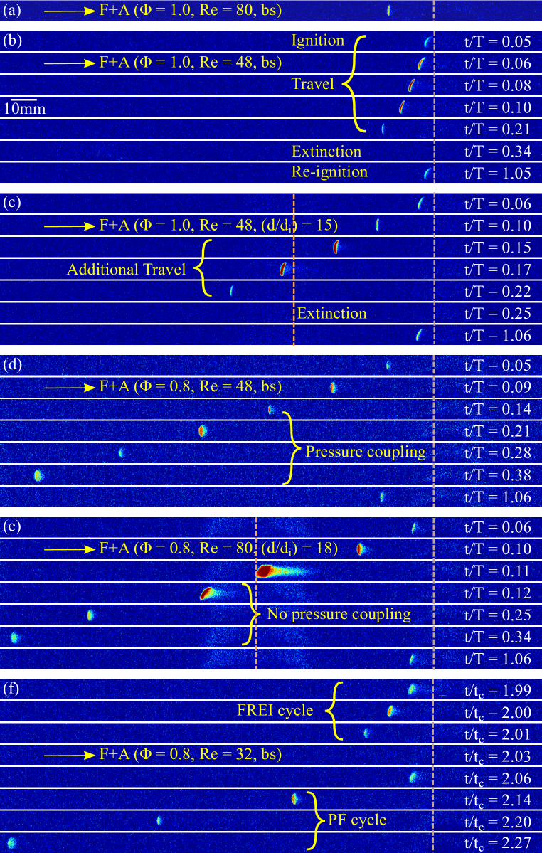
Figure 2: (a)Stationary Flames (SF). (b)Flames with repetitive extinction and ignition (FREI). (c)FREI regime flames that diverge from their baseline behavior and exhibit a second peak in their OH chemiluminescence and flame speed signals (D-FREI: Diverging FREI). (d)Propagating Flames (PF). (e)Propagating flames wherein pressure and heat release fluctuations are decoupled (D-PF: Decoupled Propagating flame). (f)Combined flame (CF) regime wherein both FREI and PF characteristics are observed. The yellow and orange dashed vertical line indicates the locations of the primary and secondary heaters, respectively. In the figure, $T$ is the characteristic time period of repetition, while $t_{c}$ is the convective time scale associated with the flow. Movies (1 to 5) in supplementary illustrate the unsteady flame regimes depicted in Fig. 2(b-f).

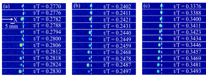
Figure 3: (a)Image sequence depicting the violent back-and-forth motion of the propagating flame at $Re=48$ for baseline case and (b)Similar back-and-forth motion of the flame front for the same Reynolds number at $d/d_{i}=18$, (c) Seamless flame front propagation at the Reynolds number of $80$ when $d/d_{i}=18$

The flame either stabilizes at a specific upstream location forming a stationary stable flame (Fig.2(a)), or continues propagating further upstream. In the latter scenario, the flame is found to exhibit two different behaviors. It may extinguish after a characteristic travel distance (Fig.2(b)), or it may persist throughout the entire length of the quartz tube only to extinguish at the upstream end where it encounters a meshed constriction (Fig.2(d)). These non-stationary flame regimes are found to repeat periodically after a characteristic time delay following extinction when the incoming mixture auto-ignites again. Accordingly, three major flame regimes can be identified: Stationary Flames (SF), Flames with repetitive extinction and ignition (FREI), and Propagating flames (PF), respectively. Fig.4 presents a regime map that depicts the identified flame regimes as a function of equivalence ratio and Reynolds number at different wall heating conditions. In the subsequent sections, the dynamics of the latter-mentioned unsteady flame regimes (FREI and PF) are discussed, initially focusing on the trends observed in the baseline case (with respect to $Re$ and $\Phi$) and then comparing them with the changes observed due to the introduction of the secondary heater at different separation distances ($d$). Although stationary steady flames are identified in the present work, further experiments are necessary to establish conclusive trends in this regime since they (Stationary flames) are expected to sustain over a wide range of Reynolds numbers above $100$ [5], which is beyond the scope of the present work.

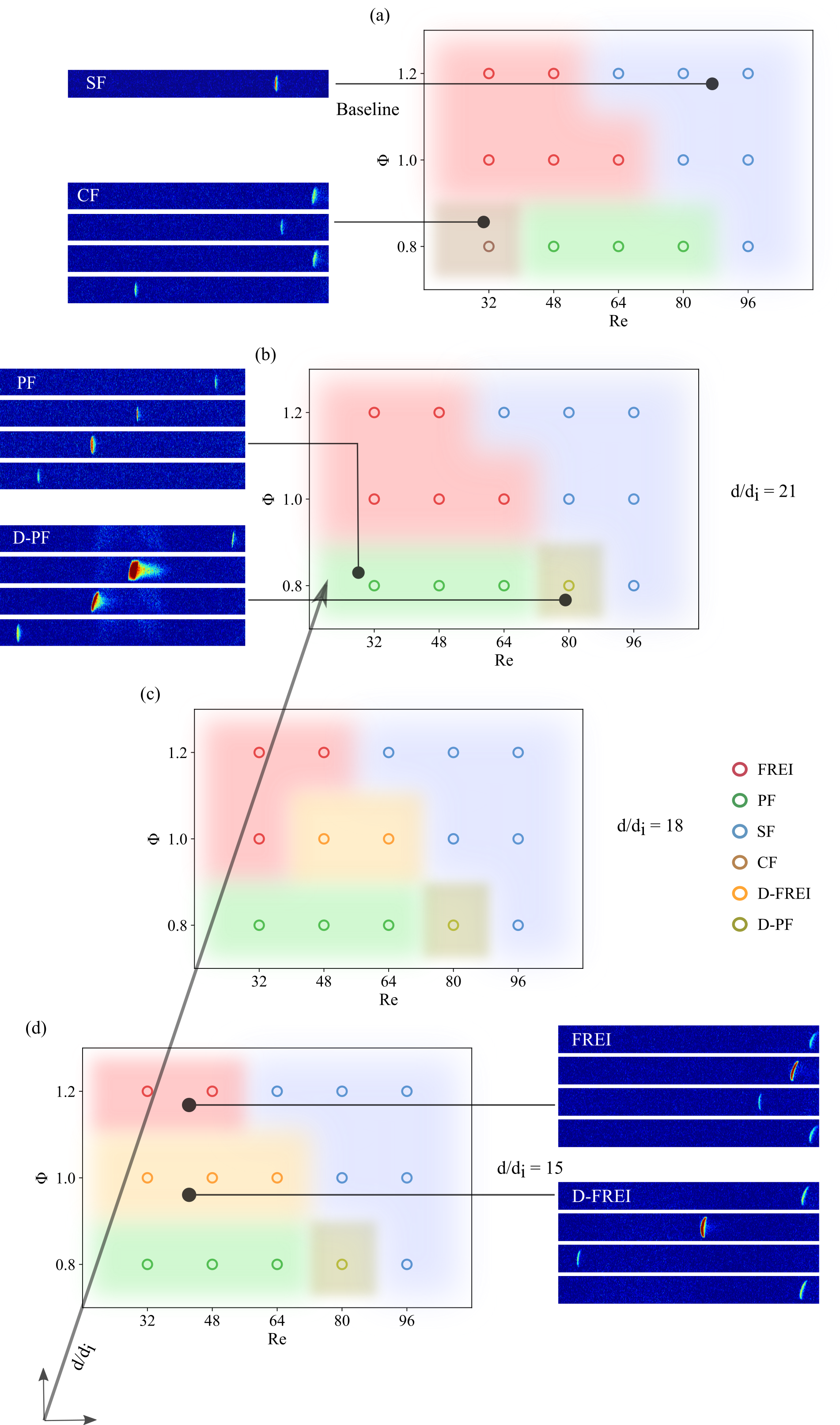
Figure 4: (a)Regime Map indicating different flame regimes observed at the baseline case. (c-d)Regime Map corresponding to $d/d_{i}$ of $21$, $18$ and $15$, respectively.

In the baseline case, the FREI regime appears at the equivalence ratio of $1.0$ and $1.2$, in the low Reynolds number regime, with the respective upper limits of $64$ and $48$ (Fig.4(a)). These flames, after auto-ignition, propagate upstream and extinguish after a characteristic travel distance. This cycle is observed to repeat itself with a characteristic frequency. The typical repetition frequency is in the order of $O(10)$ and is found to increase with Reynolds number and equivalence ratio. Both the ignition and extinction locations are found to move downstream into regions of higher wall temperatures as the Reynolds number increases. Although the ignition locations are comparable between the equivalence ratios of $1.0$ and $1.2$, the flame tends to extinguish with a shorter flame travel in regions of higher wall temperatures at $\Phi=1.2$. Introducing the secondary heater is not only found to quantitatively change the FREI descriptors (ignition-extinction locations, flame travel distance, repetition frequency) but also introduces qualitative changes in its OH chemiluminescence and flame speed profiles over a certain range of Reynolds number and equivalence ratios. At $\Phi=1.0$, the FREI dynamics significantly alter when the secondary heater is introduced at different separation distances ($d$). When a distance of 75mm ($d/d_{i}=15$) separates the secondary heater from the primary, the flame extinction location is altered, and the flame travels further upstream before extinction (Fig.2(c)). The increased flame travel is associated with an increase in the FREI cycle period and a corresponding reduction in the repetition frequency (regime depicted in Fig.4(c,d) as D-FREI or Diverging-FREI). Alongside the variations in the flame travel and FREI frequencies, an additional peak is observed in the OH chemiluminescence and flame propagation speed ($S_{f}$) signals (The first peak was associated with ignition at the downstream location). Similar behavior is observed when the secondary heater is separated from the primary by a distance of 90mm ($d/d_{i}=18$) at high Reynolds numbers ($Re\geq 48$). However, at low Reynolds numbers ($Re<48$), the flame dynamics are comparable to the baseline case, with only minor quantitative variations in FREI descriptors. For the case with $d/d_{i}=21$, the trends are similar (at all Reynolds numbers) to those observed in the low-Reynolds number regime of the case with $d/d_{i}=18$, wherein the variations with respect to the baseline case are minimal. Unlike stoichiometric conditions, at the equivalence ratio of $1.2$, the dynamics are weakly dependent on the separation distance ($d$) and only exhibit small quantitative changes (with respect to the baseline case) in the FREI descriptors across all values of $d/d_{i}$. These observations with relevant arguments are discussed in detail in section 14.

In the baseline case, propagating flames were observed at the equivalence ratio of $0.8$ between the Reynolds number range of $48$ and $80$. Propagating flames, unlike FREI, continue traveling until it reaches the upstream end of the tube, wherein it is forced to extinguish by a meshed constriction. Their ignition characteristics are similar to that observed in the FREI regime, wherein the ignition location moves downstream into regions of higher wall temperatures as $Re$ increases. However, unlike FREI, propagating flame develops instabilities during their propagation phase, that transform into violent back-and-forth motion of the flame front (Fig.2(d) and Fig.3(a)). These fluctuations are also found to be accompanied by a distinctive acoustic signal. A frequency domain analysis reveals that the fluctuations in the OH chemiluminescence (heat release rate) and pressure signals are coupled during this phase and that the frequency of oscillation is close to the natural harmonic of the combustor tube. It is interesting to note that once this coupling is established, the flame propagates upstream at an almost constant mean propagation velocity ($S_{f,ins}$), which tends to increase with the increase in the Reynolds number ($Re$). In the presence of a secondary heater, the Reynolds number range over which the regime is observed shifts between $32$ and $80$ at all values of $d$. In the presence of a secondary heater, the trends in the ignition locations and the pressure-heat release coupling are similar to those observed in the baseline case up to $Re=64$. However, at the Reynolds number of $80$, the pressure-heat release rate coupling is lost, and the flame tends to propagate upstream seamlessly without any high amplitude flame front fluctuations (Fig.2(e) and Fig.3(c), identified as D-PF or Decoupled-PF). Introducing the secondary heater is also found to elevate the peaks of the OH chemiluminescence and the flame speed signals and quantitatively alter the flame descriptors.

A combined flame regime (CF) is identified at the equivalence ratio of $0.8$ and $Re=32$ (Fig.2(f)) in the baseline configuration. The flame exhibited characteristics of both FREI and PF, wherein a series of finite travel flame cycles (flame extinction after a characteristic travel distance, similar to FREI) was followed by a propagation cycle wherein the flame traveled up to the upstream end of the tube (similar to PF). The number of FREI cycles between consecutive PF cycles was stochastic. This flame regime is synonymous with transitional flame regimes that exist at the regime boundaries of different flame types, as reported by Ju et al.[5]. This suggests a possibility of the existence of the FREI regime at Reynolds numbers below $32$ at the equivalence ratio of $0.8$, which is outside the parametric space of the present work. It is to be noted that this regime ceases to exist when the secondary heater is introduced and is only observed in the baseline configuration.

In the sections that follow (14 and 3.4.3), the above-mentioned characteristics of FREI and Propagating flames are discussed in detail with relevant scaling/mathematical arguments. However, to delve into such mathematical arguments, we need to estimate the mean flow temperature ($T_{m}$), which can act as a parameter to characterize and compare flame characteristics across the parametric space (Section 3.2).

3.2 Estimation of the Mean flow temperature

Mean flow temperature ($T_{m}$) is an estimate of the average temperature of the flow across the cross-sectional area (at a given axial distance, $x$) and can be used as a parameter to thermally characterize the ignition-extinction locations in a periodically repeating flame cycle. However, it is to be noted that the estimate of $T_{m}$ presented below is only applicable for non-reacting conditions, that is, till the section wherein the fluid packet encounters the flame. The following simplifying assumptions are used to evaluate $T_{m}$.

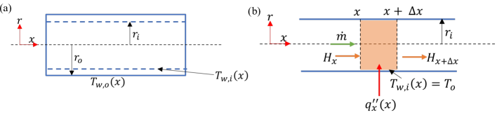
Figure 5: (a)Schematic showing the energy transfer across the tubular quartz combustor tube. (b)Schematic showing energy transfer across a control volume inside the quartz tube

1. The inner wall temperature of the combustor is maintained constant by external heating sources.
   To comprehend this assumption, let’s start off by writing down the differential form of the energy balance equation for the quartz combustor tube.

   $$\frac{\partial T}{\partial t}=\alpha\Biggl{[}\frac{\partial^{2}T}{\partial r^{2}}+\frac{1}{r}\frac{\partial T}{\partial r}+\frac{\partial^{2}T}{\partial x^{2}}\Biggr{]}$$

   Since the experiments are conducted under steady-state heating conditions, the quartz tube is in a steady state ($\frac{\partial T}{\partial t}=0$). The approximation assumes the wall-heating effect of unsteady flames to be minimal and is therefore neglected [28]. This simplifies the above equation to,

   $$\Biggl{[}\frac{\partial^{2}T}{\partial r^{2}}+\frac{1}{r}\frac{\partial T}{\partial r}+\frac{\partial^{2}T}{\partial x^{2}}\Biggr{]}=0$$

   A simple scaling analysis can now be used to deduce the temperature drop across the inner and outer walls of the quartz tube.

   $$\frac{(\triangle T)_{r}}{(\triangle r)^{2}}\sim\frac{(\triangle T)_{x}}{(\triangle x)^{2}}$$

   The inner wall temperature profile, as measured using the thermocouple, shows that the axial gradient of wall temperature is highest near the secondary heating zone where the temperature drops from $1025K$ to $300K$ ($(\triangle T)_{x}=725K$) over an axial distance of $\sim 70mm$ ($\triangle x=70mm$), which, as per the above scaling law above, would imply that $(\triangle T)_{r}\sim 0.15K$, which would correspond to the highest temperature drop in the radial direction across the thickness of the combustor tube (taking $\triangle r\sim(r_{o}-r_{i})$, where $r_{o}$ and $r_{i}$ are outer and inner wall radius of the combustor tube respectively).

   $$(\triangle T)_{r}<O(10^{0})$$

   This shows that the inner and the outer wall temperatures are comparable. It is to be noted that the above-stated inequality holds true across the entire span of parametric space explored in the current work (for all values of $Re$ and $\Phi$). This result, combined with the fact that the outer wall temperature (which is directly imposed by the dual torch and flat flame, and is not directly affected by the flow conditions inside the tube) remains constant [27, 28], implies that it is reasonable to assume that the inner wall temperature of the quartz tube (as measured using the thermocouple) is independent of the flow conditions, and can be approximated to be the same at all Reynolds numbers ($Re$) and equivalence ratios ($\Phi$).

2. Nusselt number that non-dimensionalizes the convective heat transfer between the reactant mixture flowing through the combustor and its walls is a constant.
   The hydrodynamic entrance length for the flow under study is of the order of $O(10^{-3})m$ (estimated based on the Reynolds number), and hence, the flow is fully developed as it passes through the primary and secondary heating zones. Additionally, the peclet number associated with the flow is the order $O(10)$, and hence, the effect of axial conduction inside the flow can be neglected. The energy conservation equation for the reactant mixture at steady state, thus, reduces to a balance between radial conduction and axial advection effects associated with the flow [29]. A simple scaling analysis can be used to show that, under such conditions, the Nusselt number will remain constant. The value of this constant can be evaluated to be equal to $3.66$ if we assume the inner wall temperature to remain constant [29] inside the combustor tube. For an elemental control volume of length $\triangle x$ (where $\triangle x<<L$; L: length of the combustor tube) in the flow domain (Fig.5(b)), the wall temperature (for the elemental length of $\triangle x$) can be assumed to remain constant based on the previous assumption (spatially and temporally), and thus the estimate of $Nu=3.66$ would hold true locally for that elemental control volume.

3. The mixture properties are assumed to be the same as that of air.
   Although the fluid under study is a mixture of methane and air. The composition is skewed toward air (even for the fuel-rich case, $\Phi=1.2$, the volume fraction of methane is only $\sim 10\%$); hence, it is fair to assume that the mixture properties are close to that of air [27].

To derive a formulation for the axial variation of the mean flow temperature ($T_{m}$), consider an elemental volume of length $\triangle x$ at an axial distance of $x$. Writing down an energy balance equation for the elemental control volume inside the quartz tube of inner radius $r_{i}$, we get a balance equation between radial conduction and axial convection in steady-state conditions (Fig.5(b)).

$$q^{{}^{\prime\prime}}_{w}(x)(2\pi r_{i}\triangle x)=\dot{m}[H(x+\triangle x)-H(x)]$$

where $q^{{}^{\prime\prime}}_{w}(x)$ is the wall heat flux at the axial distance of $x$, $\dot{m}$ is the mass flux through the combustor, and $H(x)$ is the specific enthalpy of the mixture at the axial distance, $x$.

Substituting for $q^{{}^{\prime\prime}}_{w}(x)$ as $h(T_{o}(x)-T_{m}(x))$, where $h$ is the co-efficient of heat transfer which is evaluated in terms of Nusselt number as, $h=((Nu)k))/(2r_{i})$; and using $H(x)=C_{p}(T)T_{m}(x)$ in the above equation, we get,

$$T_{m}(x+\triangle x)=T_{m}(x)+\triangle x\Biggl{[}\frac{\alpha(Nu)}{Ur_{i}^{2}}(T_{o}(x)-T_{m}(x))\Biggr{]}$$ (1)

where $\alpha$ is the thermal diffusivity and $U$ is the mean flow velocity of the mixture.

Since the mean flow temperature at the inlet of the quartz tube ($x=0mm$) is known, the above equation can be used to march spatially along the combustor axis to obtain the mean flow axial temperature profile. In the above equation, $Nu$ is set to a value of $3.66$ based on the assumption that in the elemental control volume of width $\triangle x$, the wall temperature remains spatially and temporally constant. The value of $\alpha$ corresponds to that estimated for air at the temperature of $T_{m}(x)$.

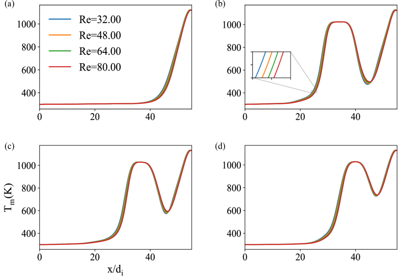
Figure 6: Mean flow temperature profiles estimated across the Reynolds number range for all wall heating conditions. (a)Baseline Case, (b)$d/d_{i}=21$, (c)$d/d_{i}=18$ and (d)$d/d_{i}=15$

Fig.6 plots the axial variation of the mean flow temperature for all the imposed wall heating conditions across the Reynolds number range from $32$ to $80$. In the range of $x/d_{i}$, where the wall temperature gradient is positive ($\frac{dT}{dx}>0$), the plots show that the mean flow temperature drops as the Reynolds number increases (Fig.6(b)), and the reverse is true when $\frac{dT}{dx}<0$. In general, the mean flow temperature profile tends to shift downstream (with respect to the wall temperature profile) with Reynolds numbers, and this downstream shift increases as the Reynolds number increases. This trend (for $\frac{dT}{dx}>0$) can be understood as follows: when $Re$ increases, the convective time scale reduces, reducing the available time for energy transfer between the wall and the fluid, resulting in lower energy transfer and, thus, lower mean flow temperatures. This implies that, as $Re$ increases, the reactants have to travel longer distances along the combustor axis to reach a given mean flow temperature.

3.3 FREI (Flames with repetitive Extinction and Ignition)

Flames with repetitive extinction and ignition appear in the low Reynolds number regime at the equivalence ratio of $1.0$ and $1.2$ as depicted in Fig.4.

3.3.1 Baseline Configuration

The typical OH signature of a FREI cycle is shown in Fig.7, plotted alongside the flame position ($x_{f}$) and flame propagation speed ($S_{f}$). There is a rapid rise in the OH chemiluminescence and the flame speed signals post auto-ignition; both reaching their peaks nearly simultaneously. Subsequently, these profiles exhibit a decaying trend as the flame propagates upstream until extinction. The discussions that follow justify the observed nature of the profile.

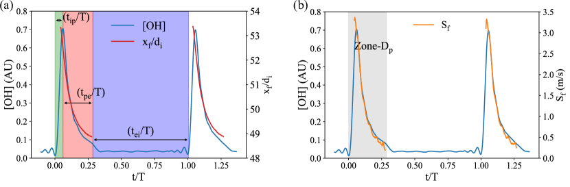
Figure 7: (a)OH chemiluminescence profile of a typical FREI regime flame plotted alongside the flame position. (b)OH chemiluminescence signal plotted alongside flame propagation speed. The plots correspond to $Re=48$ at the equivalence ratio of $1.0$ (Regime: FREI). The regions shaded in green, red, and blue are indicative of the periods associated with $t_{ip}$, $t_{pe}$, and $t_{ei}$, respectively. $T$, which normalizes the time scale, is the repetition time period of the FREI cycle. For the figure on the left, the region shaded in green, red, and purple represents the timescales of $t_{ip}/T$, $t_{pe}/T$ and $t_{pe}/T$, respectively.

A typical FREI cycle has four major events: Ignition, Peak, Extinction, and Re-ignition. Accordingly, there are three major time scales: time between ignition and peak ($t_{ip}$), time between peak and extinction ($t_{pe}$), and time between extinction and re-ignition ($t_{ei}$).

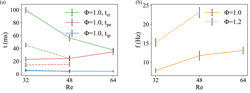
Figure 8: (a)Comparison of all the time scales involved in a FREI cycle (c)Frequency of FREI cycles at different Reynolds numbers. The solid lines in the figure correspond to $\Phi=1.0$, while the dashed lines represent $\Phi=1.2$

Fig.8(a) plots all the associated time scales of FREI cycles. In the plots, solid lines correspond to stoichiometric conditions, while dashed lines represent $\Phi=1.2$. In the discussions that follow in this section, the focus will initially be placed on the trends observed at the equivalence ratio of $1.0$ with respect to the Reynolds number. Subsequently, a comparison will be made with that observed at $\Phi=1.2$.

The time scale associated with the rise of the OH signal following ignition ($t_{ip}$) is the least dominant and tends to remain at a near-constant value across the range of Reynolds numbers. The time between extinction and re-ignition ($t_{ei}$) appears to be the most significant and exhibits a decreasing trend with $Re$. The time between peak and extinction, $t_{pe}$, although significantly lower than $t_{ei}$ at low Reynolds numbers ($Re=32$), becomes comparable to $t_{ei}$ as $Re$ increases. This is a consequence of the decreasing and increasing trends of $t_{ei}$ and $t_{pe}$ with $Re$, respectively (Fig.8(a)). Thus, comparing the magnitude and variation of different time scales across the observed Reynolds number range (as per Fig. 8(a)), $t_{ei}$ and $t_{pe}$ should dictate the variation of FREI repetition frequency with $Re$.

$$f=\frac{1}{T}=\frac{1}{t_{ip}+t_{pe}+t_{ei}}\sim\frac{1}{t_{pe}+t_{ei}}$$

While $t_{ei}$ is a strong decreasing function of $Re$ ($slope\sim-1.8ms$, Fig.8(a)), $t_{pe}$ exhibits a weak, increasing trend with an ascent rate (with respect to $Re$) of $\sim 0.3ms$ (Fig.8(a)). Since there is an order of magnitude difference between their absolute (magnitude) ascent/descent rates, the time period of the FREI cycle ($T$) is expected to follow the trend established by $t_{ei}$ and decrease with $Re$. Consequently, frequency is expected to increase with Reynolds number (following the inverse trend of $t_{ei}$ with $Re$) and is evident in Fig.8(b). Although the ascent/descent rates mentioned above correspond to the equivalence ratio of $1.0$. The qualitative arguments hold true for $\Phi=1.2$ and are apparent from the dashed plots in Fig.8 (a,b).

$$\frac{d(t_{pe})}{d(Re)}\sim 0.3ms \frac{d(t_{pe})}{d(Re)}\sim-1.8ms$$

$$\implies\frac{d(f)}{d(Re)} >0$$

A scaling argument with a physical explanation is presented later on in this section that justifies the decreasing trend of $t_{ei}$ with respect to the Reynolds number. However, it is necessary to study the trends in the ignition-extinction characteristics before delving into that.

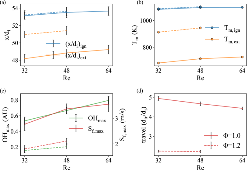
Figure 9: (a)Ignition and Extinction location are plotted alongside the corresponding mean flow temperature in (b) across the range of Reynolds numbers. (c)The variation of $(OH)_{max}$ alongside the maximum flame propagation speed $S_{f,max}$ is plotted as a function of Reynolds number. (d)Flame travel distance is plotted for different values of $Re$

For a given value of equivalence ratio, as the Reynolds number increases, the reactant mass flow rate increases, which implies an increased consumption rate of the reactants at the flame front. Since the reactant mass consumption rate ($\dot{m}$) can be expressed as a function of the flame propagation speed ($S_{f}$), unburnt gas mixture density ($\rho_{u}$), and cross-sectional area of the combustor ($A$), an increase in $\dot{m}$ would imply an increment in $S_{f}$ (since other parameters remain constant).

$$\dot{m}=\rho_{u}S_{f}A$$

However, since $S_{f}$ scales with the reaction rate ($\omega$), which in turn scales with the burnt gas temperature for a given concentration of reactant species (fixed equivalence ratio); increased mass consumption rates ($\dot{m}$) must be accompanied by increased burnt gas temperatures ($T_{b}$).

$$S_{f} \sim\omega^{1/2}$$

$$\omega\sim e^{-\frac{E}{RT_{b}}} [CH_{4}]^{a}[O_{2}]^{b}$$

In the above equation set, $E$ is the global activation energy, and $a$ and $b$ are exponents of the molar concentrations of the fuel and oxidizer species, respectively, in the global reaction rate equation.

A simple energy balance (Equation 2) between the reactants and products shows that $T_{b}$ scales with the unburnt gas temperature upstream of the flame front ($T_{u}$)

$$\Biggl{[}\sum_{k=1}^{k=m}\Biggl{(}h_{f,k}^{o}+\int_{T=T_{o}}^{T=T_{b}}C_{p,k}(T)dT\Biggr{]}_{b}\Biggr{)}=\Biggl{[}\sum_{k=1}^{k=m}\Biggl{(}h_{f,k}^{o}+\int_{T=T_{o}}^{T=T_{u}}C_{p,k}(T)dT\Biggr{]}_{u}\Biggr{)}-q_{l}$$ (2)

The above equation, $q_{l}$ represents the heat losses (on a per-mass basis), $h_{f,k}^{o}$ is the standard specific formation enthalpy of species $k$, and $C_{p,k}(T)$ is the specific heat capacity (at constant pressure) of species $k$ at the temperature $T$ and $m$ is the total number of species involved in the combustion reaction. The integral $\int C_{p,k}(T)dT$ represents the specific thermal enthalpy associated with the species $k$.

Thus, an increase in Reynolds number (causing higher reactant consumption rate) implies increased reaction rates and burnt gas temperature, which in turn necessitates an increase in the unburnt gas temperature ($T_{u}$), which implies that the mean flow temperature ($T_{m}$) upstream of the flame should be higher as $Re$ increases, and this is apparent in Fig.9(b) which shows that mean flow temperatures at the ignition location increase as $Re$ increases. Coupling the above argument with the fact that the mean flow temperature ($T_{m}$) at a location drops as $Re$ increases (Section 3.2, Fig. 6) implies that the flame should travel further downstream into regions of higher mean flow temperatures as $Re$ increases, in order to reach the temperature limit necessary to sustain combustion. The trend is evident from Fig.9(a), which shows a downstream shift in the ignition locations at higher Reynolds numbers.

As expected from the arguments above, the maxima of the flame propagation speed ($S_{f,max}$) and OH chemiluminescence signal ($OH_{max}$) increases with $Re$ (Fig.9(c)) as a consequence of increased reaction rate (to account for higher reactant consumption rate). The requirement of higher unburnt gas temperature at higher Reynolds numbers can be used to justify the trends observed in the extinction characteristics as well. Similar to that observed for the ignition locations, the extinction location shifts downstream (Fig.9(a)), and the flame extinguishes at higher mean flow temperatures (Fig.9(b)) as $Re$ increases. Following the argument stated before, an increase in $Re$ demands an increment in the unburnt gas temperatures to sustain combustion, and thus, flames are expected to extinguish at higher unburnt gas temperatures as the Reynolds number increases. The flame travel distance ($d_{tr}$), essentially the distance between ignition and extinction locations, exhibits a weak decreasing trend with increasing Reynolds number (Fig.9(d)).

An interesting observation is that the maximum flame propagation speed ($S_{f,max}$) is almost an order higher in magnitude (Fig.9(c)) compared to the laminar burning velocity of the methane-air mixture at the equivalence ratio of $1.0$ under standard conditions (upstream mixture temperature of $300K$, and $1atm$ pressure) [30]. Observed increments in flame speeds are a consequence of higher mixture mean flow temperatures upstream of the flame front.

The flame propagation speed ($S_{f}$) can be used to obtain an estimate of the preheat zone thickness, which scales as,

$$d_{ph}\sim\frac{\alpha}{S_{f}}$$ (3)

where $\alpha$ is the thermal diffusivity of the mixture ahead of the flame front at the temperature $T_{m}$. The scale of $d_{ph}$ (estimated at the peak values) is of the order of $\sim O(10^{2})\mu m$, which is almost an order lower in magnitude compared to that observed for propagating flames (discussed in Section 3.4.3).

When the flame auto-ignites and travels upstream, it encounters cold-unburnt reactants (in comparison with the temperature of the product gases, which is $\sim 2500K$); this causes the flame temperature to drop during the propagation phase. It is to be noted here that flame temperature ($T_{f}$) simply refers to the burnt gas temperature ($T_{b}$). This drop in flame temperature becomes increasingly significant as the flame continues to propagate upstream into regions of progressively lower mean flow temperatures (Fig.6). The wall heat losses accompany this effect to reduce the flame temperature further (Equation 2). The combined effect results in a decay of flame temperature along the propagation direction. This is evident in the OH chemiluminescence and $S_{f}$ profiles of the flame (Fig.7), which shows an exponential decay (Region highlighted in red in (Fig.7(a)) during the propagation phase. (As stated earlier, OH chemiluminescence and flame propagation speeds are increasing functions of flame temperature ($T_{f}$)).

The flame finally undergoes thermal quenching after a characteristic flame propagation distance when the flame temperature drops below the limit required to sustain the combustion reactions. It is to be noted here that the $d_{ph}$ estimated above is the thickness of the gas zone upstream of the flame front, preheated through axial thermal diffusion from the flame, and is responsible for transitioning the temperature of the unburnt reactants from $T_{u}$ to a critical limit required to sustain combustion reactions. Since the flame temperature decays along the propagation direction, at some point, after a characteristic travel distance, thermal diffusion from the flame front might become insufficient (due to low flame temperatures) to raise the temperature of the mixture to a limit necessary to sustain the combustion reactions, and the flame tends to undergo thermal quenching, causing flame extinction.

Following this argument, it is expected that mixtures with higher flame temperatures can sustain longer propagation distances, and this is apparent in Fig.9(d), which shows higher flame travel distance at the equivalence ratio of $1.0$, compared to that at $\Phi=1.2$. This is a consequence of low flame temperatures associated with fuel-rich conditions ($\Phi=1.2$), which leads to flame extinction at higher upstream mean flow temperatures (in comparison with $\Phi=1.0$) and is evident in Fig.9(b) as well. Similar consequences of low flame temperatures are apparent in Fig.9(c) wherein we find $S_{f,max}$ and $OH_{max}$ to be lower in fuel-rich conditions in comparison with the stoichiometric case.

The trends observed in ignition-extinction characteristics can now be used to justify the trend observed in the re-ignition time scale ($t_{ei}$). During the phase of re-ignition, the mixture has to travel a distance of $d_{tr}$ (distance between the ignition and extinction locations) to fill up the volume that was occupied by the burnt gases prior to extinction. We can estimate the increase in the time scale ($t_{ei}$) for a given velocity increment (translates to increment in Reynolds number) as,

$$\triangle t_{ei}=\frac{d_{tr}+\triangle d_{tr}}{u+\triangle u}-\frac{d_{tr}}{u}$$

where $d_{tr}$ is the re-ignition travel distance at mixture velocity $u$ and $\triangle d_{tr}$ is the change in travel distance as the mixture velocity increases by $\triangle u$. Simplifying the above equation, we get,

$$\Biggl{[}\Biggl{(}\frac{\triangle u}{u}\Biggr{)}+1\Biggr{]}\frac{\triangle t_{ei}}{t_{ei}}=\Biggl{(}\frac{\triangle d_{tr}}{d_{tr}}\Biggr{)}-\Biggl{(}\frac{\triangle u}{u}\Biggr{)}$$

Since $d_{tr}$ decreases with increase in $u$ (Fig.9(d)), $\frac{\triangle d_{tr}}{d_{tr}}$ is negative for a positive value of $\frac{\triangle u}{u}$. This implies that $\triangle t_{ei}$ is negative and that the re-ignition time scale decreases with increase in mixture velocities (increase in Reynolds number). Correspondingly, this justifies the increasing trend in the frequency of FREI cycles with $Re$ as shown in Fig.8(b). It is to be noted the arguments on the trends observed in $t_{ei}$ hold true at both equivalence ratios. The reduced flame travel ($d_{tr}$) associated with $\Phi=1.2$ (a consequence of low flame temperature) also explains the increase in repetition frequency ($f$) as a consequence of decrease in $t_{ei}$ ($t_{ei}=d_{tr}/u$) at fuel-rich conditions in comparison with the stoichiometric case (Fig.8).

3.3.2 Effect of the secondary heater

Introducing the flat flame (secondary heater) is found to divide the FREI regimes into two sub-regimes: one, wherein the flame dynamics are found only to have minor quantitative variations with respect to the baseline case (with the same qualitative behavior), while the other, wherein the qualitative profile of the OH chemiluminescence and flame speed signals associated with the flame itself is altered. We will look at the variations in the ignition-extinction characteristics to understand and characterize these sub-regimes. It is to be noted that the parametric space of equivalence ratio ($\Phi$) and Reynolds number ($Re$) over which the FREI regime was identified remains the same (as observed in the baseline case) across the entire range of wall heating conditions ($d$) explored.

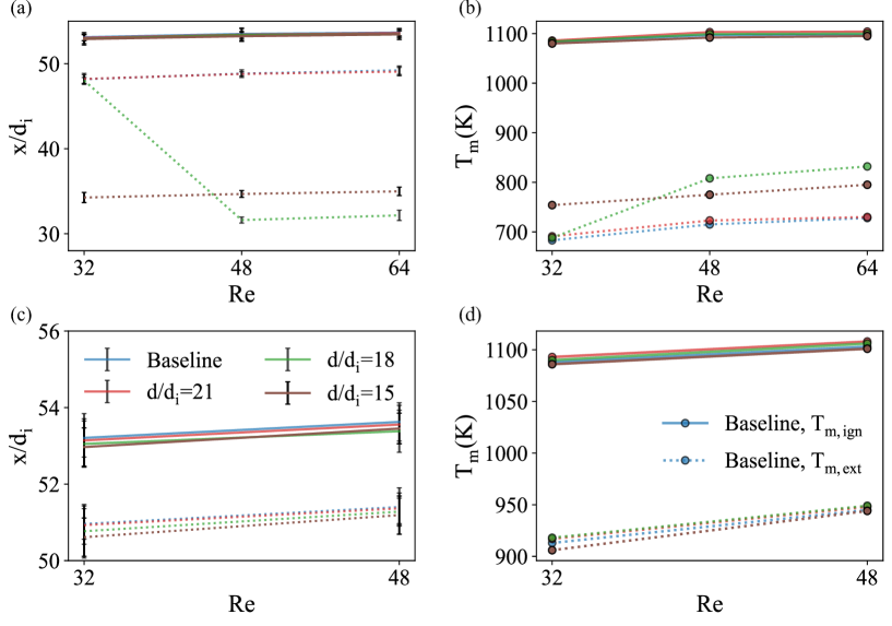
Figure 10: (a)Ignition and Extinction locations are plotted against Reynolds numbers for different wall heating conditions at the equivalence ratio of $1.0$. (b) The corresponding mean flow temperatures at these locations are plotted at different values of $Re$. (c) and (d) plots the parameters traced out in (a) and (b), respectively, for the equivalence ratio of $1.2$. The solid lines in the figure correspond to ignition locations, while dotted lines represent extinction locations

Ignition locations and their corresponding mean flow temperatures do not seem to alter significantly for different wall heating conditions (Fig.10, plotted in solid lines). The variations in $T_{m}$ (for different values of $d$) at the ignition locations are of the order of the uncertainty limit of the measured wall temperatures ($\sim 2\%$) and are not monotonic with respect to $d$, at both equivalence ratios. However, the variations in the extinction locations are prominent in a characteristic range of Reynolds numbers and separation distances ($d$) at stoichiometric conditions (Fig.10(a) and (b), plotted in dotted lines). In this characteristic range, the flame tends to exhibit an additional peak in its OH chemiluminescence and flame speed profiles. Nonetheless, at the equivalence ratio of $1.2$, the variations in extinction locations (and corresponding mean flow temperatures) are again of the order of the error limit and are insignificant, similar to their ignition characteristics (Fig.10(c) and (d)).

The flame dynamics is found to alter (or diverge from the behavior observed in the baseline configuration) for all Reynolds numbers above $32$ (from $Re=48$) when the normalized separation distance ($d/d_{i}$) is $18$ and at all Reynolds numbers for $d/d_{i}=15$. It is to be noted that this divergence from the baseline behavior (behavior in the baseline configuration) is only observed at the equivalence ratio of $1.0$. The plots in Fig.10 depict that when the flame dynamics diverges from its baseline behavior, the flame travels beyond its baseline extinction location (extinction location at the corresponding $Re$ and $\Phi$ in the baseline configuration) and extinguishes further upstream beyond the secondary heating zone. An image sequence depicting the corresponding flame dynamics is shown in Fig.2(c)

To comprehend the observed divergence in flame dynamics at certain values of $Re$ and $d/d_{i}$ at $\Phi=1.0$, let’s assess how introducing the secondary heater changes the mean flow temperature at the extinction location of the baseline case ($x_{ext,b}$) for the corresponding $Re$ and $\Phi$. Fig.11 plots the fractional change (in %) in mean flow temperatures at the extinction location of the baseline case when the secondary heater is introduced at different separation distances ($d$).

$$\Bigl{(}\text{ fractional change in $T_{m}$ at $x_{ext,b}$}\Bigr{)}_{d,\Phi,Re}=\Biggl{(}\frac{T_{m,d}(x_{ext,b})-T_{m,b}(x_{ext,b})}{T_{m,b}(x_{ext,b})}\Biggr{)}_{Re,\Phi}$$

In the above equation, $T_{m,d}(x_{ext,b})$ is the mean flow temperature at the baseline extinction location when the secondary heater is at a separation distance of $d$, while $T_{m,b}(x_{ext,b})$ is the mean flow temperature at the extinction location in the baseline case, both evaluated at a same value of $Re$ and $\Phi$. The fractional change values obtained are plotted for the entire range of equivalence ratio and Reynolds numbers at which the FREI regime is encountered (Fig.11 (b)).

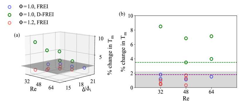
Figure 11: (a)3D scatter plot showing the % change in mean flow temperature induced at the baseline extinction locations due to introducing the secondary heater. (b) A projection of the scatter plot, showing the % change in mean flow temperature at different Reynolds numbers. The zone in grey encompasses the uncertainty limit in the measurement of wall temperature. The purple dotted horizontal line corresponds to the % change of $1.8$, which is the upper limit on the percentage change in $T_{m}$ for flames that do not show diverging flame dynamics, while the green dotted line corresponds to a % change of $3.5$, which is the lower limit on the percentage change in $T_{m}$ for diverging FREI.

Fig.11 clearly illustrates that in the cases where the flame behavior remains consistent (no diverging flame behavior) with the baseline behavior, the estimated fractional change in mean flow temperatures at the baseline extinction location remains below $\sim 1.8\%$, which is close to the uncertainty in the measurement of inner wall temperature ($sim2\%$). Conversely, cases displaying diverging behavior have their fractional change estimates exceeding this uncertainty limit. The smallest fractional change value at which we observe diverging flame dynamics ($3.5\%$) is nearly double the highest fractional change estimated in the case with no divergence ($1.8\%$). The fractional-change-estimate map distinctly divides the space into two regions, illustrating the range over which diverging flame behavior occurs as $\sim 3.5\%$ and above. It is necessary to emphasize that although a change of $\sim 3.5\%$ in the mean flow temperatures may appear modest, an increase in $T_{m}$ has a dual impact. Not only does it signify an increase in the unburnt gas temperature just ahead of the flame front at $x_{ext,b}$ (in comparison with the baseline case), but also implies a higher flame temperature immediately downstream of $x_{ext,b}$ ($x^{+}_{ext,b}$). This is because, during the propagation phase, the flame encounters mixtures with progressively lower unburnt gas temperatures; coupling this argument with the fact that the unburnt gas temperature at $x_{ext,b}$ has increased (due to the introduction of the secondary heater), shows that, the flame, prior to reaching $x_{ext,b}$, passed through a zone with temperatures greater than $T_{m,d}(x_{ext,b})$, implying a higher flame temperature just downstream of $x_{ext,b}$ (in comparison with the baseline case). Increment in both $T_{m}$ and $T_{f}$ at $x_{ext,b}$ positively contribute to flame sustenance and helps to avoid thermal quenching.

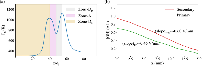
Figure 12: (a)Model Mean flow temperature profile showing different temperature zones through which the FREI regime flame propagates. (b)The plot Compares the OH chemiluminescence profile of a diverging FREI with its corresponding baseline case during the propagation phase after the flame attains its absolute maxima in OH chemiluminescence. $x_{t}$ is the position of the flame at time $t$ as measured from the flame location corresponding to the absolute maxima of the OH chemiluminescence signal in the flame propagation direction ($x_{t}$ is aligned along the $-x$ direction). The comparison laid down corresponds to the Reynolds number of $48$ at the equivalence ratio of $1.0$ between the baseline case and the case with $d/d_{i}=15$

When the flame dynamics diverge from its baseline behavior, the flame propagates further downstream beyond the baseline extinction location into the secondary heating zone. Here, as the flame propagates, it encounters a zone with mixtures having progressively higher mean flow temperatures (Region $A$ in Fig.12(a)) and, ultimately travels back into a region with mixtures having progressively decaying mean flow temperatures (Region $D_{s}$ in Fig.12(a)). These are additional zones introduced by the secondary heater. In Region $A$, since the upstream mixture temperature increases along the propagation direction, we expect a proportional trend in the flame temperature, flame speeds, and reaction rates, and this is reflected as a coupled spike in the OH chemiluminescence and the flame speed plots in Fig.13(b). The flame attains its absolute peak (in its OH chemiluminescence and the flame speed profiles) close to the exit of Region $A$ (Fig.13(b)). This peak is greater in magnitude than the one attained post-ignition. As the flame continues propagating into region $D_{s}$, the OH chemiluminescence signal and flame propagation speeds start to decay (Fig.13(b)) as the flame starts to encounter reactants with progressively lower mean flow temperature similar to that observed in the propagation phase of the baseline case.

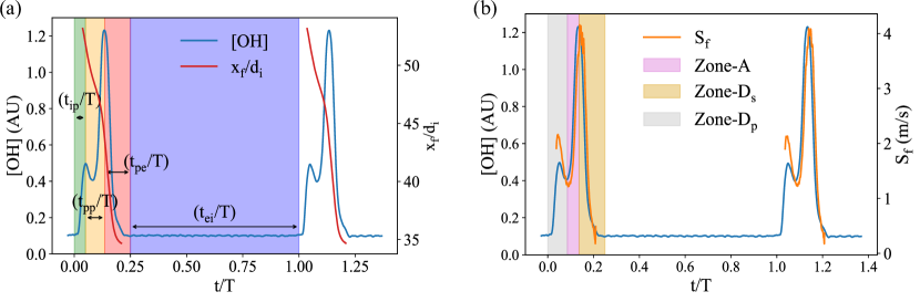
Figure 13: (a)OH signature, plotted alongside flame position for a typical FREI cycle that shows diverging flame behavior due to the introduction of the secondary heater (b)OH signature, plotted alongside flame propagation speed for the corresponding FREI cycle. The plots correspond to $Re=48$ at the equivalence ratio of $1.0$, when $d/d_{i}=15$ (Regime: D-FREI). For the figure on the left, the region shaded in green, yellow, red, and purple represents the timescales of $t_{ip}/T$, $t_{pp}/T$, $t_{pe}/T$ and $t_{pe}/T$, respectively.

It is interesting to note that the descent rate of the OH chemiluminescence signal is higher in diverging FREI compared to its baseline counterpart (Fig.12(b)). In the figure, $x_{t}$ is the position of the flame as measured from the flame location corresponding to the absolute maxima of the OH chemiluminescence signal in the flame propagation direction ($x_{t}$ is aligned along the $-x$ direction). To understand this trend in the OH chemiluminescence signal, let’s compare the mean flow temperature profiles at the extinction locations of these cases. The descent rate in the mean flow temperatures in the region $D_{s}$, wherein diverging FREI extinguishes, is around $20K/mm$, while that in the region $D_{p}$ (the region where corresponding baseline FREI extinguishes) is around $14K/mm$, at all Reynolds numbers. An estimate of the corresponding decay rate in the flame temperatures as the flame travels through these zones can be obtained by simplifying Equation 2 assuming constant and equal specific heat for all species involved in the combustion reaction.

$$T_{f}=T_{m}+\frac{\Bigl{(}\sum h_{f,k}^{o}\Bigr{)}_{reactants}-\Bigl{(}\sum h_{f,k}^{o}\Bigr{)}_{products}}{C_{p}}-\frac{q_{l}}{C_{p}}$$ (4)

$$\frac{d}{dx_{t}}(T_{f})\sim\frac{d}{dx_{t}}(T_{m})+\frac{d}{dx_{t}}\Bigl{(}\frac{-q_{l}}{C_{p}}\Bigr{)}$$

It is to be noted that in the above equation, the unburnt gas temperature is $T_{m}$, and the burnt gas temperature is the flame temperature ($T_{f}$).

Following the trend established by $T_{m}$, it is anticipated that the decay in flame temperature as the flame advances through Region $D_{s}$ will be significantly more pronounced compared to that in Region $D_{p}$ (based on the descent rates of $T_{m}$ in regions $D_{s}$ and $D_{p}$), and this justifies in the observed trends in the OH chemiluminescence signal in Fig.12(b). It is to be noted here that the effect of heat losses also contributes to the decay in flame temperature (Equation 4), thus making the descent rate in flame temperature have a higher magnitude than the descent rate in upstream mixture mean flow temperature ($T_{m}$) in both regions.

Extending our observation of the ignition-extinction characteristics, D-FREI is bound to have a change in its characteristic time scales in comparison with its baseline counterpart. It is evident from the OH chemiluminescence profile (Fig.13(a)) that flame divergence from its baseline behavior introduces an additional time scale, $t_{pp}$, which characterizes the time between the first peak (peak following ignition) and the second peak (peak due to the introduction of the secondary heater). However, a comparison of the different time scales involved reveals that the time between extinction and re-ignition ($t_{ei}$) is still the most dominant (Fig.14(a)), and thus the frequency variation with respect to Reynolds number is expected to follow the same increasing trend as that observed in the previous section (baseline case). However, $t_{pp}$ introduces a shift in the time period of diverging FREI, and this shift is reflected in the frequency plot as well (Fig.14(b)) in the form of a negative offset.

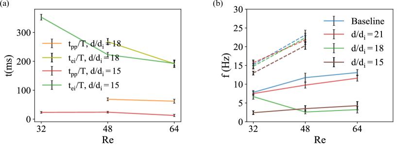
Figure 14: (a)Comparison of the normalized time scales of $t_{pp}$ and $t_{ei}$ at different Reynolds numbers for the cases that exhibit divergence from the baseline behavior. (b)FREI repetition frequency at different Reynolds numbers for all wall heating conditions. The solid lines in the figure correspond to stoichiometric conditions, while the dashed lines represent $\Phi=1.2$

3.4 Propagating Flames

Propagating flames are observed in the low-velocity regime below $Re=96$ at the equivalence ratio of $0.8$. In the baseline case, the lower Reynolds number limit at which propagating flames were observed was $Re=48$, while the lower limits for the cases with secondary heater was $Re=32$. These flames exhibit ignition characteristics similar to those observed in the FREI regime. However, they do not extinguish after a characteristic travel distance but continue propagating throughout the length of the combustor tube.

3.4.1 Baseline Configuration

The OH chemiluminescence signature of a typical propagating flame, alongside its instantaneous flame location and flame propagation speed, is plotted in Fig.15. Similar to that observed in the FREI regime, the flame auto-ignites in the high-temperature primary heating zone and starts to propagate upstream. Following ignition, there is a gradual rise in the OH chemiluminescence and flame speed signals. It is to be noted here that this ascent rate in the OH chemiluminescence signal is significantly lower with respect to that observed in the FREI regime. For comparison, the rate at which the OH signal rises post-ignition in the FREI regime at the equivalence ratio of $1.0$ and Reynolds number of $48$ is $\sim 120V/s$ (The signal obtained from the PMT is a voltage signal), with an initial flame propagation speed of $\sim 3.2m/s$, while that observed for propagating flames at the equivalence ratio of $0.8$ with the same Reynolds number is $\sim 0.37V/s$ with an initial flame propagation speed of $\sim 0.34m/s$. This order of difference magnitude in flame speeds and reaction rates (proportional to the OH chemiluminescence signal) significantly alters the dynamics of the events that follow ignition.

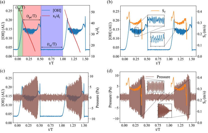
Figure 15: (a)OH chemiluminescence signature of a typical propagating flame plotted alongside flame position. (b) OH signal plotted alongside the corresponding flame propagation speeds. (c) and (d) plots the microphone signal alongside the OH chemiluminescence and flame speed signals, respectively. The profiles correspond to the Reynolds number of $48$ (Regime: PF). For the figure on the left, the region shaded in green, red, and purple represents the timescales of $t_{ip}/T$, $t_{pe}/T$ and $t_{pe}/T$, respectively.

The reduction in the flame propagation speed results in a wider pre-heat zone, as explained in Equation 3. The pre-heat zone thickness is almost an order higher for propagating flames when compared to flames in the FREI regime (estimated based on their flame propagation speeds). It is to be noted here that $S_{f}$ in propagating flames is comparable to the laminar burning velocity of methane-air mixtures under standard conditions (wherein the unburnt gases are at 300K and at atmospheric pressures), although the flame encounters unburnt mixtures with temperatures much greater than $300K$. As a consequence of low flame propagation speed, there is more time available for thermal diffusion from the flame front to raise the temperature of the upstream unburnt reactants. As a result, this reduces the susceptibility of the flame to the effects of thermal quenching (when compared to flames in the FREI regime) as the flame propagates upstream and encounters cold-unburnt reactants with progressively lower mean flow temperatures. This could potentially explain why the flame continues to propagate all the way to the upstream end of the tube, rather than extinguishing after a characteristic travel distance, as typically observed in the FREI regime.

Interestingly, propagating flames develop fluctuations in their OH chemiluminescence signal as the flame propagates into regions of low mean flow temperatures. These fluctuations grow in magnitude, turn violent over the period (Fig.15(b)), and become evident in imaging as the flame front starts moving back and forth while still continuing to propagate upstream (Fig.3(a)).

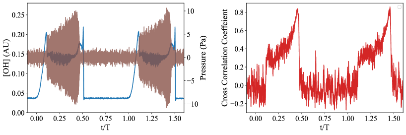
Figure S1: The figure plots the pressure and heat release rate (OH chemiluminescence) fluctuations associated with propagating flames on the left and its corresponding cross-correlation coefficient on the right. The plots correspond to the baseline configuration at the equivalence ratio of 0.8 and Reynolds number of 48 (Regime: PF). It is clear from the figure that during the propagation phase, these fluctuations are coupled.

These fluctuations are accompanied by a reduction in the mean flame propagation speeds ($S_{f}$) and OH chemiluminescence signal. Although the mean value of $S_{f}$ exhibits a gradual increase as the flame advances towards the upstream end of the tube ((Fig.15(b))), the average OH chemiluminescence signal remains near-constant throughout this phase (Fig.15(b)). When decomposed in the frequency space, it becomes evident that while these OH fluctuations initially cover a broad spectrum of low frequencies (as shown by the blue rectangle in Fig.16(a)), they eventually display only a distinct high-frequency oscillation close to the natural harmonic of the combustor tube (indicated with a black rectangle in Fig.16(a)). Interestingly, the microphone captures pressure fluctuations at the same frequency (Fig.15(c,d) and Fig.16(b,d)). The OH chemiluminescence signal, which scales with the heat release rate, and the pressure signal seem to be coupled (Fig.15(c)). A cross-correlation analysis of the pressure and heat release signal corresponding to the conditions described in Fig.15 is presented in Fig.S1 (Supplementary) and illustrates the coupling between the two signals during the propagation phase. This coupling causes the fluctuating heat release rate to add energy to the acoustic field, causing the pressure fluctuations (amplitude of the pressure signal) to grow over time, and this is evident in Fig.15(c) and (d). These pressure fluctuations, in turn, cause upstream velocity fluctuations, which lead to further heat release rate fluctuations, thus completing the thermoacoustic feedback loop. It is to be noted that (Fig.15(c)), during the coupling phase, although the pressure fluctuations tend to grow in amplitude, the amplitude of OH fluctuations tend to remain at a near constant level. This might be attributed to diffusion (momentum and thermal diffusion become increasingly relevant at small scales with high gradients in velocities and temperatures) and other mechanisms that dampen fluctuations in the heat release rate. A detailed study is necessary to understand the thermo-acoustic coupling mechanism at such small scales and is beyond the scope of the present work. The clear thermo-acoustic coupling between heat release rate and pressure is evident in the FFT plots presented in Fig.16(c) and (d). These plots highlight that the frequency corresponding to the highest spectral power density is consistent for both the PMT and microphone signals.

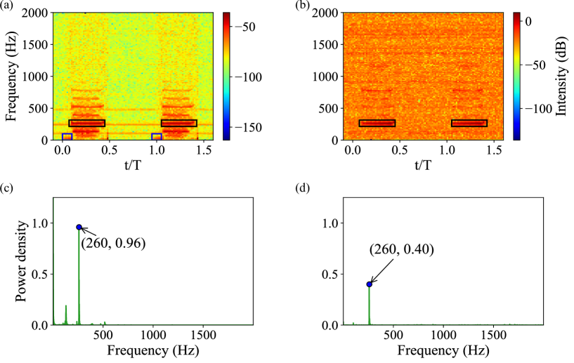
Figure 16: (a) and (b) plots the spectrogram of the OH chemiluminescence and pressure signal over the period of two propagating flame cycles, respectively. (c) and (d) plots the FFT of the corresponding signals. In the spectrogram plots, the black rectangles mark the coupling phase between the PMT and the pressure signals, while the blue rectangles depict the phase before pressure-heat release rate coupling. In this phase, low-frequency fluctuations are noticeable. The plots correspond to $Re=48$ (Regime: PF)

The amplification of pressure fluctuations doesn’t persist throughout the entire flame propagation period. They start to decay when non-linear thermo-acoustic effects start dominating. A linear analysis is presented in a later section that reveals that fluctuations at these characteristic frequencies (obtained by the spectrogram and FFT plots) grow exponentially over time. However, most of this decay phase could not be imaged, as it was confined near the upstream end of the quartz tube, which was supported by a steel structure around it for the structural integrity of the combustor; however, the OH chemiluminescence and pressure fluctuations signals were still obtained for this phase. The flame is finally quenched near the upstream end of the tube, where it encounters a meshed constriction. The process repeats again when the reactant mixture re-ignites with a characteristic time delay, generating a new propagating flame. Owing to the experimental limitations of imaging that limit us from tracking the flame position and propagation speeds, the decay phase of these thermo-acoustic oscillations is not discussed in the sections that follow and requires an independent study.

A comparison of the involved time scales, frequency of repetition, and ignition locations at different Reynolds numbers is provided in the section that follows.

3.4.2 Effect of the secondary heater

Introducing the flat flame (secondary heater) creates two important zones, one (Zone $A$ in Fig.12(a)) wherein the propagating flame encounters upstream mixtures with progressively higher mean flow temperatures and another zone with a progressively decaying mean flow temperatures in the direction of flame propagation (Zone $D_{s}$ in Fig.12(a)). The flame dynamics can alter as it travels through these zones during the propagation phase.

In the presence of the secondary heater, as the flame propagates into zone $A$ (following the gradual rise in the OH chemiluminescence signal post-ignition), the OH signal shows a rapid rise as the flame starts encountering unburnt mixtures with progressively higher mean flow temperatures along the propagation direction (Fig.17(a)). The flame attains its OH maxima close to the exit of zone $A$. Similar to the OH signal, a proportional rise and peak in the flame speeds is observed during this phase (Fig.17(b)). The flame speeds attained here are comparable to those observed in the FREI regime. As the flame propagates further into zone $D_{s}$, we see a decay in the flame speeds and OH chemiluminescence signal as the flame now starts encountering unburnt gases with progressively decaying mean flow temperatures. Unlike the FREI regime, wherein only flames within a narrow range of $Re$ and $d$ at the equivalence ratio of $1.0$, could advance through regions $A$ and $D_{s}$, in propagating flames, the behavior is observed at all Reynolds numbers. This is because, in contrast to FREI, propagating flames do not tend to extinguish after a characteristic travel distance but continue to advance to the upstream end of the tube.

Similar to that observed in the baseline case, the flame starts developing fluctuations in its heat release rate signature (OH chemiluminescence signal) as it propagates into regions of low mean flow temperatures. However, the initial fluctuations are predominantly low-frequency oscillations (with low amplitudes) that are an order away from the harmonic frequency of the combustor tube (highlighted by a blue rectangle in Fig.18(a) and (c)). The pressure signal does not seem to respond to these fluctuations, indicating the absence of thermo-acoustic coupling. From here on, the dynamics seem to vary with Reynolds number.

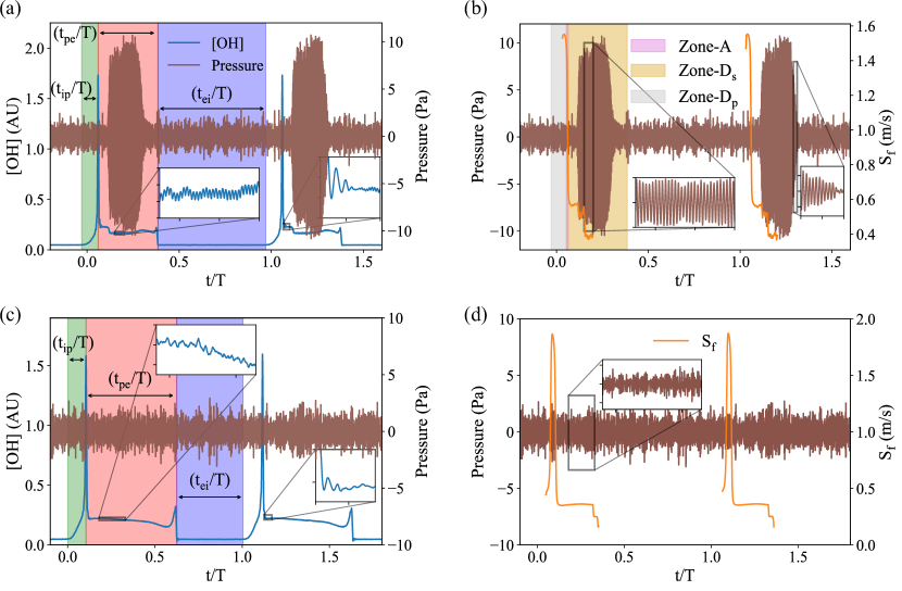
Figure 17: Pressure fluctuations are plotted alongside the OH chemiluminescence signal in (a) and (c). Pressure fluctuations are traced alongside the flame propagation speeds in (b) and (d). (a) and (b) correspond to the Reynolds number of $48$ with $d/d_{i}=18$ (Regime: PF), while (c) and (d) plots correspond to $Re=80$ at the same value of $d/d_{i}$ (Regime: D-PF)

The dynamics are observed to be similar to that of the baseline case across all heating conditions (all values of $d/d_{i}$) up to the Reynolds number of $64$. As the flame continues propagating, fluctuations at high frequencies (close to the harmonic frequency of the combustor tube) start appearing, and they develop a strong thermo-acoustic coupling (Fig.18(a) and (b)), amplifying the pressure fluctuations (Fig.17(a) and (b)) and causing the flame front to move back and forth during the propagation phase (Fig.3(b)). Similar to the baseline case, these fluctuations start decaying near the upstream end of the combustor tube.

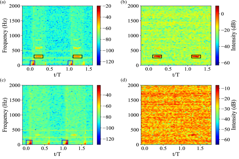
Figure 18: (a) and (b) plots the spectrogram of the OH chemiluminescence and pressure signal at the Reynolds number of $48$ and $d/d_{i}=18$ (Regime: PF), while (c) and (d) plots the same at $Re=80$ for the same separation distance (Regime: D-PF).

An additional sub-regime is identified at the Reynolds number of $80$, at which heat release rate - pressure coupling dynamics are observed to be near absent (Fig.17(c) and (d)). Fluctuations in the OH chemiluminescence (Heat release rate) and pressure signal do not seem to correspond to a specific dominant frequency (Fig.18(c) and (d)). The power associated with fluctuations (in the OH chemiluminescence and pressure signals) close to the harmonic frequency of the combustor is of the order of the noise and is not significant. The violent back-and-forth flame front oscillations are absent (Fig.3(c)), and the flame seems to propagate smoothly along the upstream direction. This sub-regime (D-PF or Decoupled-PF) is identified across the entire range of $d/d_{i}$ explored in the current work (wherein a bimodal wall temperature profile is observed) at the Reynolds number of $80$.

The rest of this section discusses the trends observed in the ignition-travel characteristics, associated time scales, and frequency of repetition of propagating flames. Similar to that observed in the FREI regime, ignition locations are comparable at different wall heating conditions (all values of $d/d_{i}$) and tend to move downstream into regions of higher mean flow temperatures as the Reynolds number increases. Fig.19(a) plots the ignition location (plotted in solid lines) and the location during the propagation phase at which the flame starts exhibiting strong thermo-acoustic coupling (plotted in dashed lines). This location was estimated based on the flame position at which Spectrogram plots of the PMT and microphone signal started showing coupled fluctuations of the order of the harmonic frequency of the combustor tube. The location will be referred to as the thermo-acoustic coupling location for the rest of the paper. For the baseline case, the thermo-acoustic coupling location tends to move downstream into regions of high mean flow temperatures as the mixture velocity increases, while the trend is reversed for the cases with the secondary heater. A similar trend is reflected in the corresponding mean flow temperatures as well (Fig.19(a), ignition mean flow temperatures are plotted in dash-dot patterns, while $T_{m}$ at the thermoacoustic coupling location is plotted in dotted lines). It is interesting to note that, although there is a significant difference in the thermo-acoustic coupling locations at different wall heating conditions (including the baseline case), the mean flow temperatures corresponding to these locations are comparable (dotted line plots in Fig.19(a)).

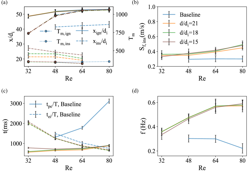
Figure 19: (a)Ignition locations and thermo-acoustic coupling locations are plotted alongside their corresponding mean flow temperatures across the Reynolds number range for different wall heating conditions. (b)The mean flame propagation speed, upstream of the thermoacoustic coupling location, is plotted against $Re$. (c)The normalized time scale of $t_{pe}$ and $t_{ei}$ are plotted against $Re$. (d)The frequency of repetition of propagating flame cycles is plotted across the explored $Re$ range

As described in the previous section, during the flame propagation phase, after the flame develops thermo-acoustic instabilities ($Re\in[32,64]$ for the cases with a secondary heater and $Re\in[48,80]$ for the baseline case), it tends to propagate upstream with a slower mean flame propagation speed. Fig.19(b) plots this mean flame propagation speed at different Reynolds numbers. It is evident from the figure that the mean flame propagation speeds increase with $Re$. They are also found to increase with the introduction of the secondary heater (with respect to the baseline case), although the variations with respect to $d/d_{i}$ are not monotonic.

Unlike FREI, in propagating flames, slow flame propagation makes the time scale associated with the flame travel ($t_{pe}$) dominant and comparable to $t_{ei}$. The variation of $t_{pe}$ and $t_{ei}$ at different Reynolds numbers is plotted in Fig.19(c). $t_{pe}$ tends to increase with Reynolds number, while $t_{ei}$ decreases with $Re$ (explained in section 14). It is interesting to note that $t_{pe}$ for the baseline case is significantly higher than the cases with a secondary heater. This is because the mean flame propagation speed is lower in the baseline case (Fig.19(b)), and the flame travel distance is greater compared to the cases with a secondary heater (Fig.19 (a) clearly shows that $x_{ins}$ for the baseline case is significantly higher (downstream) in comparison with the cases employing a secondary heater). Both of these contribute to the increment in $t_{pe}$, making it a dominant time scale in comparison with $t_{ei}$ in the baseline configuration (Fig.19(c)). However, $t_{ei}$ remains the dominant time scale for cases with a secondary heater (for Reynolds numbers below $80$).

It is evident from Fig.19(c) that while the time period of repetition in the baseline case will be dominated by the trend established by $t_{pe}$, $t_{ei}$ will dictate the trend in frequency for the cases with a secondary heater. Accordingly, we see an increasing trend in frequency with respect to $Re$ for the cases with the secondary heater (since $t_{ei}$ is the dominating time scale), while the trend is reversed in the baseline case wherein $t_{pe}$ is the dominant time scale (Fig.19(d)). For the cases that employ a secondary heater, the time scales, $t_{pe}$ and $t_{ei}$ are comparable across different values of $d/d_{i}$, and thus, the trends in frequency are expected to be similar across all bimodal wall heating conditions (all values of $d/d_{i}$). It is also clear from the figure that repetition frequency in the baseline case is significantly lower in comparison with the cases with a secondary heater, and the reason can be traced back to the significantly high values of $t_{pe}$ associated with the baseline case owing to low mean propagation velocities and increased flame travel (Fig.19(b) and (a)), as explained earlier in this section.

3.4.3 Linear acoustic analysis on Propagating flames

A linear analysis is presented in this section to theoretically estimate the coupling frequency at which pressure and heat release fluctuations interact when the flame propagates in a one-dimensional channel. The flame is visualized as a discontinuity separating the cold-unburnt reactants and the hot product gases, which is a fair assumption in the high activation energy limit when the flame thickness is negligible compared to the length scale of the combustor. A schematic of the combustor tube is provided in Fig.20.

Figure 20: A schematic depicting a model combustor used in the linear analysis

At $x=0$, the tube is assumed to be acoustically closed to account for the effect of the meshed constriction at the upstream end, and the combustor has an open end at $x=L$. The flame position is marked by $x_{f}$. For simplicity, a step temperature profile is assumed for the gas mixture inside the combustion chamber. The mixture is assumed to remain at the ambient temperature ($T_{u}$; unburnt gas temperature) till it encounters the flame, at which point it attains a temperature of $T_{b}$ (burnt gas temperature) and continues to remain in this limit till the downstream end of the tube. Although a huge approximation, it can still help understand trends and compute the thermo-acoustic modes that amplify and become unstable [31, 32]. It is to be noted here that since the speed of sound depends on the fluid temperature ($c=\sqrt{\gamma RT}$), the acoustic waves travel at different velocities before and after the flame. $c_{u}$ and $c_{b}$ are the acoustic velocities in the unburnt ($x\in(0,x_{f})$) and burnt gas regions ($x\in(x_{f},L)$), respectively. For low Mach number flames like that encountered here, pressure variation across the flame can be neglected, and combustion can be assumed to be isobaric ([33]).

For performing the linear acoustic analysis, all the flow variables are expressed as a summation of their base flow quantities (denoted by superscript $0$) and acoustic perturbation terms (superscript $1$).

$$a=a_{0}+a_{1}$$

To derive the evolution equation for the perturbation terms, a few more simplifying assumptions are necessary to be laid down. The equations are derived for a quiescent region ($u_{0}=0$) with constant base flow density ($\rho_{0}=constant$) and base flow entropy ($s_{0}=constant$). The mixture is assumed to be an ideal gas with negligible diffusion effects (momentum and thermal) and body force terms. To make the formulation applicable to the present case, the analysis should be performed in the reference frame of the unburnt mixture (making $u_{0}=0$).

Substituting the flow variables in terms of their base-flow and perturbation components alongside the above-mentioned approximations, the conservation equations (mass, momentum, and energy) yield the following set of differential equations in 1D.

$$\rho_{0}\frac{\partial u_{1}}{\partial t}+\frac{\partial p_{1}}{\partial x} =0$$ (5)

$$\frac{\partial p_{1}}{\partial t}+\gamma p_{0}\frac{\partial u_{1}}{\partial x} =(\gamma-1)\rho_{0}\dot{q_{1}}$$ (6)

where $\rho_{0}$ is the baseline density, $p_{0}$ is the baseline pressure, $\gamma$ is the ratio of specific heats, $u_{1}$ and $p_{1}$ are the acoustic velocities and pressure and $\dot{q_{1}}$ is the heat release rate fluctuation. It is to be noted here that $\dot{q_{1}}=0$ in the unburnt and the burnt gas regions and is non-zero only in the region occupied by the flame, which is of negligible volume in the high activation energy limit described above. Thus, we can formulate equations for $p_{1}$ and $u_{1}$ in the unburnt and burnt gas region with $\dot{q_{1}}=0$, and then impose jump boundary conditions at the interface of the two regions to introduce the effect of the flame.

The above equations can be simplified for the burnt and unburnt gas regions with $\dot{q_{1}}=0$ to obtain the acoustic wave equation as,

$$\frac{1}{c^{2}}\biggl{(}\frac{\partial^{2}p_{1}}{\partial t^{2}}\biggr{)}-\nabla^{2}p_{1}=0$$

The solution to the above set of differential equations reduce to the form,

$$p_{1}(x,t)=Ae^{ik(x-x_{f})+i\omega t}+Be^{-ik(x-x_{f})+i\omega t}$$

$$u_{1}(x,t)=\frac{-A}{\rho c}e^{ik(x-x_{f})+i\omega t}+\frac{B}{\rho c}e^{-ik(x-x_{f})+i\omega t}$$

where $A$ and $B$ are constants, $k$ is the wave number and $\omega$ is the angular frequency. Wave number and angular frequency can be related as $\omega=kc$. It is to be noted that $A$, $B$, $k$, and $c$ differ in the burnt and the unburnt zones. Writing these equations explicitly for the burnt and unburnt regions, we get,

$$p_{1}(x,t)=\begin{cases}A_{u}e^{ik_{u}(x-x_{f})+i\omega t}+B_{u}e^{-ik_{u}(x-x_{f})+i\omega t}&\text{$x\in(0,x_{f})$}\\ A_{b}e^{ik_{b}(x-x_{f})+i\omega t}+B_{b}e^{-ik_{b}(x-x_{f})+i\omega t}&\text{$x\in(x_{f},L)$}\end{cases}$$ (7)

$$u_{1}(x,t)=\begin{cases}\frac{-A_{u}}{\rho_{u}c_{u}}e^{ik_{u}(x-x_{f})+i\omega t}+\frac{B_{u}}{\rho_{u}c_{u}}e^{-ik_{u}(x-x_{f})+i\omega t}&\text{$x\in(0,x_{f})$}\\ \frac{-A_{b}}{\rho_{b}c_{b}}e^{ik_{b}(x-x_{f})+i\omega t}+\frac{B_{b}}{\rho_{b}c_{b}}e^{-ik_{b}(x-x_{f})+i\omega t}&\text{$x\in(x_{f},L)$}\end{cases}$$ (8)

Evaluating the boundary condition and jump conditions across the flame will yield us a dispersion relation to evaluate $\omega$. At $x=0$, the acoustic velocity is zero since the upstream end is approximated as a closed-end, giving us,

$$A_{u}e^{-ik_{u}x_{f}}-B_{u}e^{ik_{u}x_{f}}=0$$ (9)

The pressure perturbation goes to zero at the open end ($x=L$) since the end is open to the atmosphere.

$$A_{b}e^{ik_{b}(L-x_{f})}+B_{b}e^{-ik_{b}(L-x_{f})}=0$$ (10)

In the high activation energy limit, wherein we approximate the flame to be a discontinuity at $x=x_{f}$, it can be demonstrated that the $p_{1}$ would remain the same across the flame. The approximation can be derived by integrating equation 5 over the infinitesimally small control volume ($V_{f}$) surrounding the flame (approaching the limit where the size of this control volume tends to zero).

$$\lim_{{V_{f}\to 0}}\Biggl{[}\int_{V_{f}}\Bigl{(}\rho_{0}\frac{\partial u_{1}}{\partial t}+\frac{\partial p_{1}}{\partial x}\Bigr{)}dV=0\Biggr{]}\quad\implies dp_{1}=0$$

$$\implies A_{u}+B_{u}=A_{b}+B_{b}$$ (11)

To derive the jump conditions in perturbation velocities across the flame, we need to consider the governing equation presented before.

$$\frac{\partial p_{1}}{\partial t}+\gamma p_{0}\frac{\partial u_{1}}{\partial x}=(\gamma-1)\rho_{0}\dot{q_{1}}$$

Integrating the above equation in the volume occupied by the flame, we get,

$$u_{1}(x=x^{+}_{f})-u_{1}(x=x^{-}_{f})=\frac{(\gamma-1)}{c^{2}_{u}A}\int_{V_{f}}\dot{q_{1}}dV$$ (12)

The right-hand side of the above equation can now be approximated using the $n-\tau$ model ([34]) as,

$$\frac{(\gamma-1)}{c^{2}_{u}A}\int_{V_{f}}\dot{q^{\prime}}dV=nu_{1}(x_{f},t-\tau)$$ (13)

It is to be noted here that $n$ and $\tau$ in the above equation are unknown parameters that need separate evaluation. Substituting Equation 13 in Equation 12 and simplifying, we get

$$\bigl{[}1+ne^{-i\omega\tau}\bigr{]}(A_{u}-B_{u})-\Gamma(A_{b}-B_{b})=0$$ (14)

where $\Gamma=\frac{\rho_{u}c_{u}}{\rho_{b}c_{b}}$. Equations 9, 10, 11 and 14 represents a system of linear equations with $A_{u}$, $B_{u}$, $A_{b}$ and $B_{b}$ as the variables. Since the right-hand side of all the equations are zero, non-trivial solutions can exist only when the determinant of the co-coefficients matrix is zero.

$$\begin{vmatrix}e^{-ik_{u}x_{f}}&-e^{ik_{u}x_{f}}&0&0\\ 0&0&e^{ik_{b}(L-x_{f})}&e^{-ik_{b}(L-x_{f})}\\ 1&1&-1&-1\\ \bigl{[}1+ne^{-i\omega\tau}\bigr{]}&-\bigl{[}1+ne^{-i\omega\tau}\bigr{]}&-\Gamma&\Gamma\end{vmatrix}=0$$

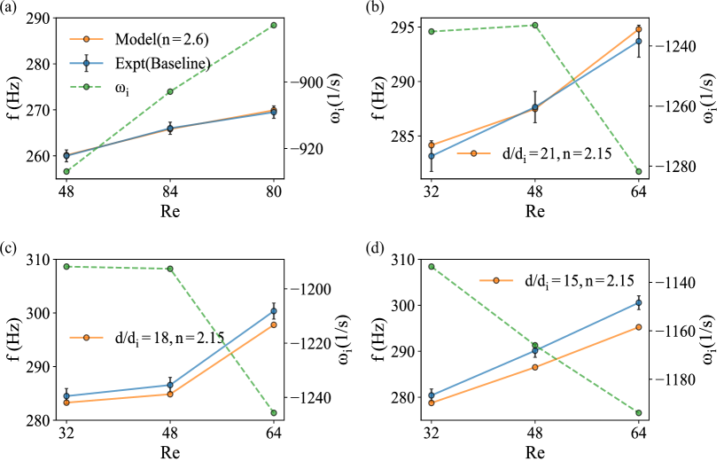
Figure 21: Theoretical estimate of the thermoacoustic frequency in comparison with the experimentally observed coupling frequency between heat release rate and pressure fluctuations. $\omega_{i}$, which characterizes the growth rate of instability, is also plotted alongside. (a) corresponds to the baseline case. (b), (c) and (d) corresponds to $d=105mm$, $d=90mm$ and $d=75mm$ respectively

The above equation, when simplified, yields the dispersion relation for $\omega$. Setting both the real and imaginary parts of the above equation to zero, we get a system of coupled non-linear equations. The obtained system for equations relates $\omega$ with the flame position $x_{f}$, with $n$ and $\tau$ as parameters that characterize the flame heat release rate response to upstream velocity perturbations. Although these parameters require individual assessment, which is outside the scope of the present work, we are going to work around the problem by iteratively estimating these parameters. The value of $\tau=-T/4$, where, $T$ is the time period of the fluctuations, was found to very closely reproduce the experimental data with the value of $n=2.15$ for the cases with a secondary heater, and $n=2.6$ for the baseline case.

The theoretical values of $\omega$ corresponding to different flame locations (that correspond to different Reynolds numbers from the experimental data) are obtained and compared against the experimentally obtained frequencies in Fig.21. It is to be noted here that the flame location used to theoretically estimate $\omega$ corresponds to the thermoacoustic coupling locations (plotted in Fig.19(a)).

The theoretical estimates are in good agreement with the experimental results. It should be noted here that $\omega_{i}$ (evaluated theoretically) is negative at all Reynolds numbers, and this has an important consequence. We know that $(p_{1},u_{1})\sim e^{i\omega t}$, which can be written down as $(p_{1},u_{1})\sim e^{-\omega_{i}t}e^{i\omega_{r}t}$. The equation implies that fluctuations corresponding to the frequency of $\omega_{r}$ will tend to grow exponentially over time when $\omega_{i}$ is negative, implying that fluctuations at these frequencies are unstable. However, the results hold true only in the linear framework, wherein perturbation terms are very small in comparison with the bulk flow variables. Non-linear effects start dominating as the amplitude of the fluctuations grows and might be the reason for the instabilities to decay as the flame approaches the upstream end of the tube.

3.5 Combined Flames

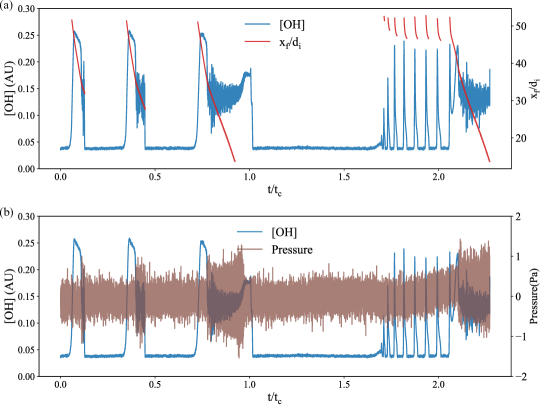
Figure 22: (a)OH chemiluminescence of the flame plotted alongside the flame position for $Re=32$ and $\Phi=0.8$ (Regime: CF). (b)Corresponding pressure signal plotted alongside its OH chemiluminescence signature.

At the Reynolds number of $32$ and equivalence ratio of $0.8$, a flame exhibiting characteristics of both FREI and PF was observed. The OH chemiluminescence signature of the flame is plotted in Fig.22, alongside its corresponding instantaneous flame position and flame propagation speeds. The image sequence depicting the flame dynamics is presented in Fig.2(f).It is quite evident from the figure that there is no periodicity in the observed flame dynamics. Convective time scale ($t_{c}$) is hence used to non-dimensionalize time and represent time-series variation in Fig.22. The flame tends to exhibit a series of finite travel FREI cycles following a propagating flame cycle (wherein the flame travels to the upstream end of the combustor tube). The number of FREI cycles between consecutive propagation flame cycles was stochastic and was found not to exhibit a characteristic repetition frequency. Not only was the flame behavior qualitatively switching between FREI and PF, but FREI descriptors (extinction locations, flame travel distance) showed quantitative changes between consecutive FREI cycles.

As the observation of this flame type was limited to a single data point ($Re=32$, $\Phi=0.8$), further data analysis was not possible to establish conclusive trends. It requires an independent study that deals with mesoscale flame dynamics at $Re<32$.

4 Conclusion

The study explores the dynamics of premixed flames in mesoscale channels subjected to a bimodal wall heating profile, wherein the separation distance between the heating peaks was varied (by varying the relative distance between two external heating sources that impose the bimodal profile), and the dynamics were observed over a wide range of Reynolds numbers and equivalence ratios. The dynamics were compared against a baseline case that employed a single heater to produce a unimodal wall heating profile. Three major flame regimes were identified: a steady stationary flame regime and two unsteady flame regimes. The work is centered around these unsteady flames. Depending on the operating equivalence ratio, different types of unsteady flames were observed: one, wherein the flame goes through a succession of ignition, propagation, extinction, and re-ignition events (Flames with repetitive extinction and ignition, FREI; observed at the equivalence of $1.0$ and $1.2$), and the other, wherein the flame travels the entire length of the combustor tube (Propagating flames; observed at the equivalence ratio of $0.8$). FREI was identified between the Reynolds numbers of $32$ and $64$ at the equivalence ratio of $1.0$ and between $32$ and $48$ at the equivalence ratio of $1.2$ (at all wall temperature conditions); while propagating flames were observed for $Re\in[32,80]$ at all bimodal heating conditions, and between $48$ and $80$ in the baseline configuration. The above-mentioned unsteady flame regimes repeat after a characteristic period, and the repetition frequency increases with the Reynolds number and equivalence ratio. Further trends in the ignition-extinction characteristics, OH chemiluminescence, and flame speeds have been discussed in detail for both regimes. FREI displays a flame bifurcation behavior in a characteristic range of Reynolds numbers and separation distances (axial distance between the temperature peaks), at an equivalence ratio of $1.0$. This divergence in flame behavior introduces additional peaks in their OH chemiluminescence and flame speed profiles, altering their qualitative description. Similarly, propagating flames also undergo a shift in their qualitative flame description when subjected to a bimodal wall heating profile. Propagating flames display a characteristic thermo-acoustic coupling during the propagation phase at frequencies close to the natural frequency of the combustor tube. However, this pressure-heat release rate coupling ceases to exist beyond a critical Reynolds number limit under bimodal wall heating conditions. The work also presents a simplified linear acoustic model to predict the thermoacoustic coupling frequency in propagating flames.

Declaration of Interests

The authors report no conflict of interest.

Supplementary

References

- [1] A. C. Fernandez-Pello, Micropower generation using combustion: Issues and approaches, Proc. Combust. Inst. 29 (2002) 883–899.
- [2] K. Maruta, Micro and mesoscale combustion, Proc. Combust. Inst. 33 (2011) 125–150.
- [3] N. S. Kaisare, D. G. Vlachos, A review on microcombustion: Fundamentals, devices and applications, Prog. Energ. Combust 38 (2012) 321–359.
- [4] S. Zimmermann, P. Krippner, A. Vogel, J. Müller, Miniaturized flame ionization detector for gas chromatography, Sensor. Actuat. B-Chem 83 (2002) 285–289.
- [5] Y. Ju, K. Maruta, Microscale combustion: Technology development and fundamental research, Prog. Energ. Combust 37 (2011) 669–715.
- [6] S. A. Lloyd, F. J. Weinberg, A burner for mixtures of very low heat content, Nature 251 (1974) 47–49.
- [7] C. J. Evans, D. C. Kyritsis, Experimental Investigation of the Effects of Flame Phenomenology on the Wall Temperature Distribution of Mesoscale Nonadiabatic Ducts, Combust. Sci. Technol 183 (2011) 847–867.
- [8] C. Miesse, R. Masel, M. Short, M. Shannon, Experimental observations of methane–oxygen diffusion flame structure in a sub-millimetre microburner, Combust. Theor. Model 9 (2005) 77–92.
- [9] K. T. Kim, D. H. Lee, S. Kwon, Effects of thermal and chemical surface–flame interaction on flame quenching, Combust. Flame 146 (2006) 19–28.
- [10] K. Maruta, T. Kataoka, N. I. Kim, S. Minaev, R. Fursenko, Characteristics of combustion in a narrow channel with a temperature gradient, Proc. Combust. Inst. 30 (2005) 2429–2436.
- [11] K. Maruta, J. K. Parc, K. C. Oh, T. Fujimori, S. S. Minaev, R. V. Fursenko, Characteristics of Microscale Combustion in a Narrow Heated Channel, Combust. Explo. Shock+ 40 (2004) 516–523.
- [12] A. Fan, S. Minaev, E. Sereshchenko, R. Fursenko, S. Kumar, W. Liu, K. Maruta, Experimental and numerical investigations of flame pattern formations in a radial microchannel, Proc. Combust. Inst. 32 (2009) 3059–3066.
- [13] F. Richecoeur, D. C. Kyritsis, Experimental study of flame stabilization in low Reynolds and Dean number flows in curved mesoscale ducts, Proc. Combust. Inst. 30 (2005) 2419–2427.
- [14] Y. Ju, B. Xu, Theoretical and experimental studies on mesoscale flame propagation and extinction, Proc. Combust. Inst. 30 (2005) 2445–2453.
- [15] D. A. Kessler, M. Short, Ignition and transient dynamics of sub-limit premixed flames in microchannels, Combust. Theor. Model 12 (2008) 809–829.
- [16] T. L. Jackson, J. Buckmaster, Z. Lu, D. C. Kyritsis, L. Massa, Flames in narrow circular tubes, Proc. Combust. Inst. 31 (2007) 955–962.
- [17] J. A. Bieri, V. N. Kurdyumov, M. Matalon, The effect of gas expansion on edge flames stabilized in narrow channels, Proc. Combust. Inst. 33 (2011) 1227–1234.
- [18] C. J. Evans, D. C. Kyritsis, Operational regimes of rich methane and propane/oxygen flames in mesoscale non-adiabatic ducts, Proc. Combust. Inst. 32 (2009) 3107–3114.
- [19] F. Nicoud, T. Poinsot, Thermoacoustic instabilities: Should the Rayleigh criterion be extended to include entropy changes?, Combust. Flame 142 (2005) 153–159.
- [20] T. David P, Experimental investigation of the flow field during combustion in narrow circular ducts, Ph.D. thesis, University of Illinois at Urbana-Champaign (2012).
- [21] X. Kang, R. J. Gollan, P. A. Jacobs, A. Veeraragavan, Numerical study of the effect of wall temperature profiles on the premixed methane–air flame dynamics in a narrow channel, RSC. Adv 7 (2017) 39940–39954.
- [22] V. Ratna Kishore, S. Minaev, M. Akram, S. Kumar, Dynamics of premixed methane/air mixtures in a heated microchannel with different wall temperature gradients, RSC. Adv 7 (2017) 2066–2073.
- [23] G. Vadlamudi, S. K. Thirumalaikumaran, S. Basu, Insights into the dynamics of wake flame in a freely falling droplet, Phys. Fluids 33 (2021) 123306.
- [24] K. Pandey, S. Basu, G. V, A. Potnis, K. Chattopadhyay, Self-tuning and topological transitions in a free-falling nanofuel droplet flame, Combust. Flame 220 (2020) 144–156.
- [25] S. K. Thirumalaikumaran, G. Vadlamudi, S. Basu, Insight into flickering/shedding in buoyant droplet-diffusion flame during interaction with vortex, Combust. Flame 240 (2022) 112002.
- [26] A. Savitzky, M. J. E. Golay, Smoothing and Differentiation of Data by Simplified Least Squares Procedures., Anal. Chem 36 (1964) 1627–1639.
- [27] A. Di Stazio, C. Chauveau, G. Dayma, P. Dagaut, Combustion in micro-channels with a controlled temperature gradient, Exp. Therm. Fluid. Sci 73 (2016) 79–86.
- [28] A. Di Stazio, C. Chauveau, G. Dayma, P. Dagaut, Oscillating flames in micro-combustion, Combust. Flame 167 (2016) 392–394.
- [29] A. Bejan, Convection Heat Transfer, John Wiley Sons, Ltd, New Jersey, 2013, pp. 96–167.
- [30] R. J. Varghese, H. Kolekar, V. R. Kishore, S. Kumar, Measurement of laminar burning velocities of methane-air mixtures simultaneously at elevated pressures and elevated temperatures, Fuel 257 (2019) 116120.
- [31] P. Clavin, P. Pelcé, L. He, One-dimensional vibratory instability of planar flames propagating in tubes, J. Fluid. Mech 216 (1990) 299–322.
- [32] P. Pelcé, D. Rochwerger, Vibratory instability of cellular flames propagating in tubes, J. Fluid. Mech 239 (1992) 293–307.
- [33] C. K. Law, Combustion Physics, Cambridge University Press, 2006, p. 234–302.
- [34] M. Schmid, R. S. Blumenthal, M. Schulze, W. Polifke, T. Sattelmayer, Quantitative Stability Analysis Using Real-Valued Frequency Response Data, J. Eng. Gas. Turb. Power 135 (2013) 121601.