Measurement of flow coefficients in high-multiplicity $p$+Au, $d$+Au and ³He$+$Au collisions at $\sqrt{s_{{}_{\mathrm{NN}}}}$=200 GeV

Abstract

Flow coefficients ($v_{2}$ and $v_{3}$) are measured in high-multiplicity $p$+Au, $d$+Au, and ³He$+$Au collisions at a center-of-mass energy of $\sqrt{s_{{}_{\mathrm{NN}}}}$ = 200 GeV using the STAR detector. The measurements are conducted using two-particle correlations with a pseudorapidity requirement of $|\eta|<$ 0.9 and a pair gap of $|\Delta\eta|>1.0$. The primary focus of this paper is on the analysis procedures and methods employed, especially the subtraction of non-flow contributions. Four well-established non-flow subtraction methods are applied to determine $v_{n}$, and their validity is verified using the HIJING event generator. The $v_{n}$ values are compared across the three collision systems at similar multiplicities, which allows for cancellation of final state effects and isolation of the impact of the initial geometry. While the $v_{2}$ values display differences among these collision systems, the $v_{3}$ values are largely similar, consistent with the expectations of subnucleon fluctuations in the initial geometry. The ordering of $v_{n}$ differs quantitatively from previous measurements obtained using two-particle correlations with a larger rapidity gap; this difference could be partially attributed to the effects of flow decorrelations in the rapidity direction.

I Introduction

High-energy collisions of heavy nuclei, such as gold at RHIC and lead at the LHC, give rise to a hot and dense state of matter composed of strongly interacting quarks and gluons, referred to as the Quark-Gluon Plasma (QGP) Busza et al. (2018). This QGP experiences rapid expansion in the transverse direction, converting initial spatial nonuniformities into significant anisotropic particle flow within the transverse momentum ($p_{\mathrm{T}}$) space. This flow, spanning a wide range of pseudorapidity $\eta$, can be accurately described by viscous relativistic hydrodynamic equations with extremely low viscosity Gale et al. (2013); Heinz and Snellings (2013). Therefore, the QGP is often likened to a nearly inviscid liquid, known as the “perfect fluid”.

Experimentally, the anisotropic flow is manifested as a harmonic modulation of particle distribution in the azimuthal angle $\phi$ for each event, given by the equation:

$$\frac{dN}{d\phi}\propto 1+2\sum_{n=1}^{\infty}v_{n}(p_{\mathrm{T}})\cos(n(\phi-\Psi_{n}))\;.$$ (1)

Here, the magnitude $v_{n}$ and orientation $\Psi_{n}$ of the $n^{\mathrm{th}}$-order harmonic flow are commonly represented by the flow vector $V_{n}\equiv v_{n}e^{in\Psi_{n}}$. The flow coefficients with the most significant magnitudes are the elliptic flow $v_{2}$ and the triangular flow $v_{3}$. However, the direct measurement of the event-wise distribution described by Eq. 1 is limited by the finite number of particles produced in each event, and the flow coefficients are obtained via a two-particle azimuthal correlation method:

$$\frac{dN_{\mathrm{pairs}}}{d\Delta\phi}\propto 1+2\sum_{n=1}^{\infty}c_{n}(p_{\mathrm{T}}^{\mathrm{t}},p_{\mathrm{T}}^{\mathrm{a}})\cos(n\Delta\phi)\;,$$ (2)

where it is anticipated that $c_{n}(p_{\mathrm{T}}^{\mathrm{t}},p_{\mathrm{T}}^{\mathrm{a}})=v_{n}(p_{\mathrm{T}}^{\mathrm{t}})v_{n}(p_{\mathrm{T}}^{\mathrm{a}})$, assuming a factorization behavior for $v_{n}$ extracted from two distinct $p_{\mathrm{T}}$ ranges Aad et al. (2012). To mitigate short-range “non-flow” correlations stemming from sources such as jet fragmentation and resonance decays, a pseudorapidity gap is typically employed between particles labeled as “t” (trigger) and “a” (associated).

Naturally, questions arise regarding the minimum system size at which the “perfect fluid” behavior can be observed, as well as whether QGPs created with various sizes exhibit consistent properties. To address these questions, a series of measurements have been conducted in several small systems, ranging from $p$+$p$ Khachatryan et al. (2010); Aad et al. (2016); Khachatryan et al. (2017) to $p$+A Chatrchyan et al. (2013); Abelev et al. (2013); Aad et al. (2013); Adare et al. (2013, 2015); Abdulameer et al. (2023); Abdulhamid et al. (2023), and $\gamma$+A collisions Aad et al. (2021a). These measurements unveiled notable anisotropic flow in all of these systems. A decade-long debate ensued regarding whether the observed flow originates from final-state effects (FS), resulting from the collective response to the initial geometrical fluctuations in each event, or if it stems from initial-state effects (IS), such as intrinsic momentum correlations within the nuclear wavefunction at high energies. The latter can persist even in the absence of final-state interactions Dusling et al. (2016); Schenke (2021). Recent theoretical efforts have demonstrated that IS models, primarily rooted in gluon saturation physics, exhibit relatively short-range features in $\eta$ Schenke et al. (2022), and fail to reproduce detailed $p_{\mathrm{T}}$ dependence Schenke et al. (2015); Mace et al. (2018) and multi-particle correlations Mace et al. (2019). Consequently, the current consensus within the scientific community leans toward the FS interpretation of collective flow in small systems.

It is crucial to recognize that the final-state perspective does not necessarily imply the applicability of hydrodynamics and the presence of a perfect fluid. A continuing discussion revolves around whether the medium formed in these systems can be characterized as a perfect fluid with well-defined transport properties or if it constitutes a collection of partons undergoing only a few average scatterings without achieving hydrodynamic or thermal equilibrium He et al. (2016); Kurkela et al. (2019); Romatschke (2018); Kurkela et al. (2021). Even within the hydrodynamics framework, certain calculations introduce a “pre-flow” phase, where partons undergo free streaming before enabling the hydrodynamic evolution  Weller and Romatschke (2017). However, a common thread across these models is the notion that harmonic flow originates from the initial spatial anisotropies, characterized by eccentricity vectors with magnitude $\varepsilon_{n}$ and direction $\Phi_{n}$, denoted as ${\mathcal{E}}_{n}=\varepsilon_{n}{e}^{{\textrm{i}}n\Phi_{n}}$.

In large collision systems, model calculations have established an approximate linear relationship between flow and eccentricity for both elliptic and triangular flow Gardim et al. (2012); Niemi et al. (2013):

$$v_{n}=k_{n}\varepsilon_{n},\;n=2,3\;.$$ (3)

In this context, response coefficients $k_{n}$, encompassing all final state effects remain constant for events with similar particle multiplicities. However, the validity of Eq. 3 and its hydrodynamic interpretation is not as firmly established in small collision systems. The non-hydrodynamic approaches mentioned earlier can significantly alter the response coefficients $k_{n}$ and their $p_{\mathrm{T}}$ dependencies. A significant challenge persists in experimentally distinguishing between non-equilibrium transport and hydrodynamics. Unambiguous confirmation of perfect fluid behavior in these small systems requires making this distinction with certainty.

Table 1: The values of $\varepsilon_{2}$ and $\varepsilon_{3}$ in central collisions (requiring either impact parameter $b<2$ fm or 0–5% centrality), obtained from Glauber models Alver et al. (2008) including nucleon Nagle et al. (2014); Aidala et al. (2019); Abdulhamid et al. (2023) or subnucleon fluctuations Welsh et al. (2016). They are defined either as simple average, $\left\langle\varepsilon_{n}\right\rangle$ Nagle et al. (2014); Aidala et al. (2019), or the root-mean-square values, $\sqrt{\left\langle\varepsilon_{n}^{2}\right\rangle}$, which take into account event-by-event fluctuations. The values have negligible statistical uncertainties. The values in 0–2% or 0–10% centralities are not shown, but they are nearly identical to those quoted for 0–5%.

	Nucleon	Nucleon	Subnucleon
	Glauber Nagle et al. (2014); Aidala et al. (2019)	Glauber Alver et al. (2008); Abdulhamid et al. (2023)	Glauber Welsh et al. (2016)
	$b<2$ fm	0–5% centrality	0–5% centrality
	$\left\langle\varepsilon_{2}\right\rangle$  $\left\langle\varepsilon_{3}\right\rangle$	$\sqrt{\left\langle\varepsilon_{2}^{2}\right\rangle}$  $\sqrt{\left\langle\varepsilon_{3}^{2}\right\rangle}$	$\sqrt{\left\langle\varepsilon_{2}^{2}\right\rangle}$  $\sqrt{\left\langle\varepsilon_{3}^{2}\right\rangle}$
3He+Au	0.50  0.28	0.53  0.33	0.54  0.38
$d$+Au	0.54  0.18	0.59  0.28	0.55  0.35
$p$+Au	0.23  0.16	0.28  0.23	0.41  0.34

One reason for encountering this challenge lies in the absence of quantitative control over the initial conditions and the associated $\varepsilon_{n}$ in small systems. An important consideration pertains to whether each projectile nucleon should be regarded as a single smooth blob or as multiple blobs comprising gluon fields (as illustrated in the top panels of Fig. 1). Notably, the flow data observed in $p$$+$$p$ collisions at the LHC cannot be explained without invoking significant spatial fluctuations at the subnucleon level, which necessitates considering multiple distinct “hot spots” within each colliding proton Mäntysaari and Schenke (2016). Such subnucleonic fluctuations are anticipated to be important in extremely-asymmetric collision systems like $p$+A or $d$+A collisions (although their dependence on $\sqrt{s_{\mathrm{NN}}}$ remains unknown).

In the case of $p$$+$Au, $d$$+$Au, and ³He$+$Au collisions within the RHIC small system scan, the $\varepsilon_{n}$ values naturally depend on the assumed structure of the projectile $p$, $d$, and ³He, respectively. Table 1 shows that the differences of $\varepsilon_{3}$ among the three systems, in particular, are sensitive to whether the nucleons in the projectiles are treated as one smooth distribution without fluctuation from nucleon to nucleon, or fluctuating distribution with varying pattern from nucleon to nucleon. When modeling nucleons as single smooth blobs, the resulting $\varepsilon_{3}$ values in $p$$+$Au and $d$$+$Au collisions are reduced, and they become significantly smaller than the $\varepsilon_{3}$ in ³He$+$Au collisions Nagle et al. (2014). Conversely, considering each nucleon as three spatially-separated blobs around valence quarks yields larger, yet much closer, $\varepsilon_{3}$ values for the three collision systems Welsh et al. (2016). The impact of considering subnucleon-level fluctuations on $\varepsilon_{3}$ in $d$$+$Au collisions is depicted by comparing the two top panels of Fig. 1.

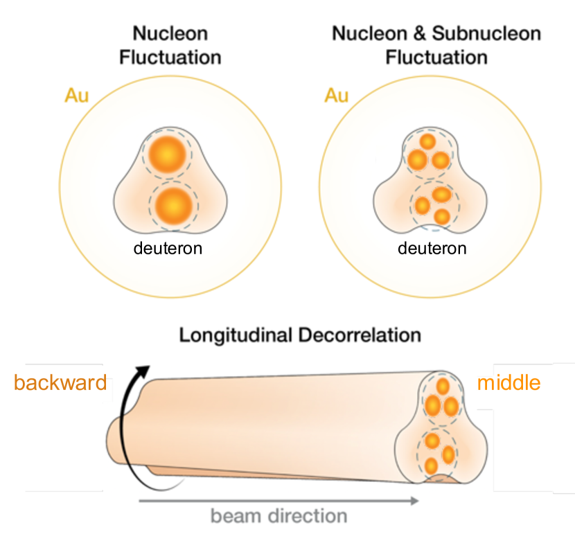
Figure 1: Cartoon illustrating the interplay of three potential sources contributing to the triangular eccentricity $\varepsilon_{3}$ in asymmetric collisions like $d$$+$Au: fluctuations in nucleon position (top-left), fluctuations in nucleon position along with their quark and gluon constituents (top-right), and fluctuations of the initial geometry defined by the overlap between deuteron and Gold nuclei along the beam direction, commonly referred to as longitudinal decorrelations (bottom).

Another crucial aspect of the initial condition that introduces significant uncertainty is its longitudinal structure (as depicted in the bottom panel of Fig. 1). Experimental measurements in Pb+Pb, Xe+Xe, and $p$+Pb collisions at the LHC Khachatryan et al. (2015); Aaboud et al. (2018); Aad et al. (2021b), along with supporting model studies Bozek et al. (2011); Jia and Huo (2014); Bozek and Broniowski (2016); Pang et al. (2016); Shen and Schenke (2018); Bozek and Broniowski (2018); Zhao et al. (2022), have revealed significant fluctuations in the shape of the initial geometry along the $\eta$ direction within the same individual events. These fluctuations lead to significant decorrelation of the eccentricity vector as a function of $\eta$. Consequently, the extracted $v_{n}$ values from the two-particle correlation method depend on the chosen $\eta$ range for selecting the particle pairs. A larger $\eta$ gap results in a smaller extracted $v_{2}$ signal. The decorrelation effect is more pronounced for $v_{3}$ and is particularly notable in smaller collision systems Khachatryan et al. (2015); Zhao et al. (2023).

Distinguishing the effects of fluctuations at the nucleon and subnucleon levels, as well as those arising from longitudinal decorrelations in collision geometry, is imperative to convincingly establish the creation of QGP in these small systems and to extract its properties.

To comprehend the origin of collectivity in small systems, particularly the role of collision geometry, RHIC has undertaken a scan of $p$$+$Au, $d$$+$Au, and ³He$+$Au collisions. The PHENIX Collaboration measured $v_{2}$ and $v_{3}$ through correlations between particles in the central rapidity region and the backward (Au-going) rapidity region Aidala et al. (2019); Acharya et al. (2022). The pseudorapidity gap $\Delta\eta$ ranges from three units to one unit depending on the method used. The results reveal a hierarchy $v_{3}^{\scriptsize\mbox{$p$$+$Au}}\approx{v_{3}^{\scriptsize\mbox{$d$$+$Au}}}\approx\frac{1}{3}v_{3}^{\scriptsize\mbox{${}^{3}$He$+$Au}}$, consistent with model calculations employing a version of nucleon Glauber initial conditions Nagle et al. (2014) . Recently, STAR also measured $v_{2}$ and $v_{3}$ using correlations of particles closer to mid-rapidity while requiring a $\Delta\eta$ gap of one unit Abdulhamid et al. (2023). The findings suggest similar values of $v_{3}$ at comparable particle multiplicities in the three collision systems. The $v_{3}$ values in ³He$+$Au are comparable between the two experiments, yet they differ notably in $p$$+$Au and $d$$+$Au. This discrepancy could potentially be attributed to a weaker longitudinal decorrelation in the STAR measurement, although recent model estimates account for only about half of the observed differences Zhao et al. (2023).

Another operational difference between the two experiments is that PHENIX did not perform an explicit non-flow subtraction. The rationale behind this decision is that the non-flow component is reduced due to the large pseudorapidity gap between the middle and backward detectors, and any residual non-flow contributions are then covered by systematic uncertainties Aidala et al. (2019). Conversely, in the STAR analysis, larger non-flow contamination is expected owing to its smaller pseudorapidity gap, necessitating a careful estimation and subsequent subtraction of non-flow contributions Abdulhamid et al. (2023).

The primary objective of this paper is to provide a detailed description of the methods and non-flow subtraction procedure that culminated in the results published in Ref. Abdulhamid et al. (2023). Furthermore, we conduct an extensive comparison with hydrodynamic model calculations.

II Data and Event Activity Selection

II.1 Event Selection

The datasets employed for this analysis include $p$$+$$p$, $p$$+$Au, $d$$+$Au, and ³He$+$Au collisions at a center-of-mass energy of $\sqrt{s_{{}_{\mathrm{NN}}}}=200$ GeV, collected by the STAR experiment during the years 2014, 2015, and 2016. Minimum Bias (MB) triggers are used for data collection in both $p$$+$$p$ and ³He$+$Au collisions, while $p$$+$Au and $d$$+$Au collisions utilize both MB and High Multiplicity (HM) triggers.

The MB triggers in $p$$+$$p$, $p$$+$Au, and $d$$+$Au collisions require a coincidence between the east and west Vertex Position Detectors (VPD) Llope et al. (2014), which cover a rapidity range of 4.4 $<|\eta|<$ 4.9. For ³He$+$Au collisions, the MB triggers require coincidences among the east and west VPD and the Beam-Beam Counters (BBC) Bieser et al. (2003). Additionally, at least one spectator neutron in the Zero Degree Calorimeter (ZDC) Adler et al. (2001) on the Au-going side is required. The rapidity coverage of these detectors is $3.3<|\eta|<5.1$ and $\eta<-6.5$, respectively. The MB trigger efficiency ranges from 60% to 70% for $p$$+$Au, $d$$+$Au, and ³He$+$Au collisions systems. For MB $p$$+$$p$ collisions, this efficiency was estimated to be around 36% Adamczyk et al. (2012).

In $p$$+$Au and $d$$+$Au collisions, the HM triggers require a minimum number of hits in the Time Of Flight (TOF) detector Llope (2012), in conjunction with the MB trigger criteria.

For offline analysis, events are selected based on their collision vertex position $z_{\mathrm{vtx}}$ relative to the Time Projection Chamber (TPC) center along the beam line. The chosen position falls within 2 cm of the beam spot in the transverse plane. The specific $z_{\mathrm{vtx}}$ ranges are optimized for each dataset, guided by distinct beam tuning conditions: 20 cm, 30 cm, 15 cm, and 30 cm for $p$$+$$p$, $p$$+$Au, $d$$+$Au, and ³He$+$Au data, respectively. Moreover, to suppress pileup and beam background events in the TPC, a selection based on the correlation between the number of tracks in the TPC and those matched to the TOF detector is applied.

II.2 Track Reconstruction and Selection

Charged particle tracks are reconstructed within $|\eta|<1$ and $p_{\mathrm{T}}>0.2$ GeV/$c$ by the TPC. Track quality adheres to established STAR analysis standards: tracks are required to have at least 16 fit points in the TPC (out of a maximum of 45), with a fit-point-to-possible-hit ratio exceeding 0.52. To minimize contributions from secondary decays, tracks are subject to a requirement that their distance of closest approach (DCA) to the primary collision vertex is less than 2 cm. Additionally, a valid track must be associated with a hit in the TOF detector or a signal in at least one strip layer in the Heavy Flavor Tracker (HFT) detector Szelezniak (2015). The TOF and HFT detectors offer faster response times compared to the TPC, effectively mitigating the effects of pileup tracks associated with multiple collisions that accumulate during TPC drift time. To ensure high track reconstruction efficiency, only tracks within $|\eta|<0.9$ are utilized in the correlation analysis.

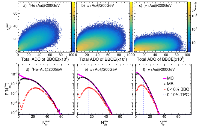
Figure 2: Top row: Plot depicting $N_{\mathrm{ch}}^{\mathrm{raw}}$ vs. $\Sigma{Q_{\mathrm{BBCE}}}$ in minimum bias (MB) ³He$+$Au, $d$$+$Au, and $p$$+$Au collisions at $\sqrt{s_{{}_{\mathrm{NN}}}}=200$ GeV. Bottom row: Distribution of $N_{\mathrm{ch}}^{\mathrm{raw}}$ in each system. The black circles, red circles, and blue dashed lines correspond to MB, top 0–10% event activity selected from BBCE and TPC, respectively. The pink solid curves indicate the generated multiplicity distribution derived from a Monte Carlo Glauber model fit (see text).

The track reconstruction and matching efficiency are evaluated using the established STAR embedding technique Abelev et al. (2010). This technique involves generating charged particles within a Monte Carlo generator, and subsequently subjecting them to a GEANT model representation of the STAR detector. The simulated detector signals are then merged with real data to capture the effects of the actual detector occupancy conditions. Subsequently, these merged events are reconstructed using the same offline reconstruction software utilized for real data production.

The tracking efficiency is assessed by comparing the reconstructed tracks with the simulated input tracks. Specifically, tracking efficiency within the TPC exhibits minimal dependence on $p_{\mathrm{T}}$ for values exceeding 0.5 GeV/$c$, reaching a plateau at approximately 0.9 across all collision systems. Applying a requirement for matching to the TOF detector reduces this plateau value to approximately 0.74.

II.3 Event Activity Selection

Our objective is to measure harmonic flow in $p/d/^{3}$He+Au collision events with large charged particle multiplicity or event activity. To achieve this, events are categorized into percentile ranges known as centrality classes, based on their apparent multiplicity as detected by a specific instrument. The most central events, situated within the top 0–10% or the top 0–2% of the multiplicity distribution, are chosen for subsequent analysis and comparison.

The default centrality classes are defined by employing the observed charged track multiplicity, $N_{\mathrm{ch}}^{\mathrm{raw}}$, within the pseudorapidity region $|\eta|<$ 0.9 and transverse momentum range of 0.2 $<p_{\mathrm{T}}<$ 3.0 GeV/$c$ in the TPC Anderson et al. (2003). These charged particle tracks are required to have a matched hit in the TOF detector. A Monte Carlo Glauber model, along with one of two distinct assumptions about particle production, is used to simulate the multiplicity distribution, which is then fitted to the $N_{\mathrm{ch}}^{\mathrm{raw}}$ to determine the centrality percentiles.

The first approach is based on the two-component model for particle production Kharzeev and Nardi (2001), where the number of sources for particle production is assumed to be

$$N_{s}=\left[(1-x)\frac{N_{\rm part}}{2}+xN_{\rm coll}\right],$$ (4)

where $x$ is the fraction of the second component. The number of participants, $N_{\mathrm{part}}$, and number of collisions, $N_{\rm coll}$, are extracted from the PHOBOS Glauber Monte Carlo simulation Alver et al. (2008). In the second approach, the $N_{s}$ is assumed to follow a power law dependence on $N_{\mathrm{part}}$, $N_{s}=\mbox{$N_{\mathrm{part}}$}^{\alpha}$.

The multiplicity fluctuation is incorporated via the Negative Binomial Distributions (NBD) for each source,

$$P_{\rm NBD}(\mu,k;n)=\frac{\Gamma(n+k)}{\Gamma(n+1)\Gamma(k)}\cdot\frac{(\mu/k)^{n}}{(\mu/k+1)^{n+k}},$$ (5)

where $n$ is the generated multiplicity, and $\mu$ and $k$ are free parameters. The inefficiency for triggering events with a single source is assumed to be $\varepsilon$.

The multiplicity of an event at the generator level $N_{\mathrm{ch}}^{\mathrm{mc}}$ is obtained by summing $n$ for all $N_{s}$ sources. The corresponding multiplicity after accounting for trigger inefficiency, denoted by $N_{\mathrm{ch}}^{\mathrm{obs}}$, is also obtained.

The distribution of $N_{\mathrm{ch}}^{\mathrm{obs}}$ is then fitted to measured $N_{\mathrm{ch}}^{\mathrm{raw}}$ distributions for each specific collision system. The trigger inefficiency $\varepsilon$ and NBD parameters $\mu$ and $k$ are adjusted to achieve an optimal global fit. This procedure also yields a multiplicity distribution at the generated level, $N_{\mathrm{ch}}^{\mathrm{mc}}$, from which we can determine the centrality percentiles.

Examples of $N_{\mathrm{ch}}^{\mathrm{mc}}$ from the first approach are displayed in the lower panels of Fig. 2 in the three collision systems. The apparent deviations of data at low $N_{\mathrm{ch}}^{\mathrm{raw}}$ values are attributable to the inefficiency of the MB triggers, while the simulated distribution agrees with the data at large $N_{\mathrm{ch}}^{\mathrm{raw}}$ values. The values of $\left\langle N_{\mathrm{ch}}^{\mathrm{raw}}\right\rangle$ are found to be slightly different between the two approaches. For the top 0–10% centrality interval, they amount to a 4% difference in $p$$+$Au collisions and 3% in $d$/³He+Au collisions.

In order to examine the potential auto-correlation between event selection and flow signal, an alternative event activity selection is introduced as a cross-check. This selection relies on the signal from the BBC on the Au-going side (denoted as BBCE) within a pseudorapidity range of $-5.0<\eta<-3.3$. For instance, the 0–10% event classes are characterized as the top 10% of the total charge registered by the BBCE, denoted as $\Sigma Q_{\rm BBCE}$. The correlation between $N_{\mathrm{ch}}^{\mathrm{raw}}$ and $\Sigma Q_{\rm BBCE}$ is illustrated in the upper panels of Fig. 2 for Minimum Bias (MB) $p$$+$Au, $d$$+$Au, and ³He$+$Au collisions. A broad correlation is observed in all three systems, implying that events in a narrow range of $N_{\mathrm{ch}}^{\mathrm{raw}}$ can have a large spread in $\Sigma Q_{\rm BBCE}$ and vice versa. Corresponding $N_{\mathrm{ch}}^{\mathrm{raw}}$ distributions for MB and 0–10% events, selected via TPC and BBC, are displayed in the lower panels.

Table 2 provides the efficiency-corrected multiplicities, $\left\langle N_{\mathrm{ch}}\right\rangle$, for MB $p$$+$$p$ and the 0–10% most central $p$/$d$/³He$+$Au collisions, selected using both $N_{\mathrm{ch}}^{\mathrm{raw}}$ and $\Sigma Q_{\rm BBCE}$. Additionally, the table presents values for the 0–2% most central $p$/$d$+Au collisions, selected with TPC-based centrality. The systematic uncertainties on $\left\langle N_{\mathrm{ch}}\right\rangle$ arise mainly from uncertainties in charged pion reconstruction efficiency, evaluated through the earlier mentioned embedding procedure. The additional PID dependence of the reconstruction efficiency associated with $K^{\pm}$ and (anti-)protons are estimated from embedding and the known particle ratios Abelev et al. (2009). The total uncertainty associated with the efficiency correction is estimated to be around 5%.

Note that the $\left\langle N_{\mathrm{ch}}\right\rangle$ value quoted for MB $p$$+$$p$ collisions are not corrected for the trigger inefficiency, and therefore should be treated as the value for selected events.

	MB $p$$+$$p$	$p$$+$Au	$d$$+$Au	3He$+$Au
$\left<N_{\mathrm{ch}}\right>$	4.7$\pm$0.3	0–10% from TPC
		21.9$\pm$1.1	35.6$\pm$1.8	47.7$\pm$2.4
		0–2% from TPC
		34.1$\pm$1.7	46.4$\pm$2.3	-
		0–10% from BBC
		15.7$\pm$0.8	27.6$\pm$1.4	41.6$\pm$2.1

Table 2: The efficiency-corrected average multiplicity, $\left\langle N_{\mathrm{ch}}\right\rangle$, for MB $p$$+$$p$, 0–10% most central $p$/$d$/³He$+$Au collisions, as well as 0–2% most central $p$$+$Au and $d$$+$Au collisions using TPC-based centrality. The values obtained for 0–10% BBC-based centrality are also shown.

III Methodology for $v_{n}$ extraction

III.1 Two-particle correlation function and per-trigger yield

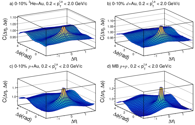
Figure 3: The normalized two-particle correlation function presented as a function of $\Delta\eta$ and $\Delta\phi$ for the trigger and associated particles within the 0.2 $<p_{\mathrm{T}}<$ 2.0 GeV/$c$ range in central $p$$+$Au, $d$$+$Au, ³He$+$Au, and MB $p$$+$$p$ collisions at $\sqrt{s_{{}_{\mathrm{NN}}}}=200$ GeV.

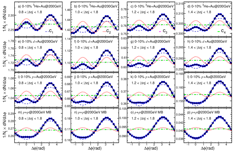
Figure 4: The per-trigger yield displayed as a function of $\Delta\phi$ in central ³He$+$Au (top row), $d$$+$Au (second row), $p$$+$Au (third row), and MB $p$$+$$p$ (bottom row) collisions for particles with $0.2<p_{\mathrm{T}}^{\mathrm{t}},p_{\mathrm{T}}^{\mathrm{a}}<2.0$ GeV/$c$. The plots are provided for four different $\Delta\eta$ selections, moving from left to right. The color curves represent the Fourier components obtained from the Fourier expansion of the per-trigger yield.

The analysis measures two-particle correlations as functions of the relative pseudorapidity, $\Delta\eta$, and relative azimuthal angle, $\Delta\phi$ Adare et al. (2008). Trigger particles are defined as charged particle tracks within $|\eta|<0.9$ and within the specific $p_{\mathrm{T}}^{\mathrm{t}}$ range of $0.2<p_{\mathrm{T}}^{\mathrm{a}}<2.0$ GeV/$c$. Pairs of particles are then formed by pairing each trigger particle with the remaining charged particle tracks that satisfy $|\eta|<0.9$, and $0.2<p_{\mathrm{T}}^{\mathrm{a}}<2.0$ GeV/$c$. This leads to a maximum gap of $|\Delta\eta|<1.8$ between the pairs. The track reconstruction efficiency is applied to individual particles.

The two-dimensional two-particle correlation function, $C(\Delta\eta,\Delta\phi)$, is calculated using the formula:

$$C(\Delta\eta,\Delta\phi)=\frac{\int{B(\Delta\eta^{\prime},\Delta\phi^{\prime})d\Delta\phi^{\prime}d\Delta\eta^{\prime}}}{\int{S(\Delta\eta^{\prime},\Delta\phi^{\prime})d\Delta\phi^{\prime}d\Delta\eta^{\prime}}}\frac{S(\Delta\eta,\Delta\phi)}{B(\Delta\eta,\Delta\phi)}\;,$$ (6)

where $S(\Delta\eta,\Delta\phi)$ and $B(\Delta\eta,\Delta\phi)$ represent the pair distributions from same-event and mixed-event samples, respectively. Mixed-event pairs are formed by combining tracks from two different events with similar centrality and similar $z_{\mathrm{vtx}}$, as detailed in Ref. Adare et al. (2008). The correlation functions $C(\Delta\eta,\Delta\phi)$ are obtained for different collision systems with centrality selection based on the TPC multiplicity. The resulting correlation functions from MB events are displayed in Fig. 3 for $p_{\mathrm{T}}^{\mathrm{t}}$ in the range of $0.2<p_{\mathrm{T}}^{\mathrm{t}}<2.0$ GeV/$c$ (examples for other $p_{\mathrm{T}}^{\mathrm{t}}$ ranges are shown in Appendix VIII). Notably, a ridge-like structure around $\Delta\phi=0$ and along the $\Delta\eta$ direction is clearly observed in central $d$$+$Au and ³He+Au collisions, and possibly in $p$$+$Au collisions, whereas it is absent in MB $p$$+$$p$ collisions.

To obtain one-dimensional correlation functions, $C(\Delta\phi)$, the two-dimensional correlation functions are projected by integrating over $\Delta\eta$:

$$C(\Delta\phi)=\frac{\int{B(\Delta\phi^{\prime})d\Delta\phi^{\prime}}}{\int{S(\Delta\phi^{\prime})d\Delta\phi^{\prime}}}\frac{S(\Delta\phi)}{B(\Delta\phi)}\;,$$ (7)

where $S(\Delta\phi)$ and $B(\Delta\phi)$ are obtained by integrating $S(\Delta\eta,\Delta\phi)$ and $B(\Delta\eta,\Delta\phi)$ using four distinct ranges of $|\Delta\eta|$: $|\Delta\eta|>$ 0.8, 1.0, 1.2, and 1.4. The per-trigger yield, denoted as $Y(\Delta\phi)$, is then defined as:

$$Y(\Delta\phi)\equiv\frac{1}{N_{\mathrm{t}}}\frac{dN}{d\Delta\phi}=\frac{C(\Delta\phi)\int{S(\Delta\phi)d\Delta\phi}}{N_{\mathrm{t}}\int{d\Delta\phi}}\;,$$ (8)

where $N_{\mathrm{t}}$ is the number of trigger particles after efficiency correction.

Figure 4 illustrates $Y(\Delta\phi)$ obtained for MB $p$$+$$p$ and the 0–10% most central $p$$+$Au, $d$$+$Au, and ³He+Au collisions in the four $|\Delta\eta|$ ranges, with $p_{\mathrm{T}}$ of trigger particles in the range of $0.2<p_{\mathrm{T}}^{\mathrm{t}}<2.0$ GeV/$c$. One-dimensional correlation functions for other $p_{\mathrm{T}}^{\mathrm{t}}$ ranges can be found in Figs. 21–24 in Appendix VIII.

After a gap cut of $\mbox{$\Delta\eta$}_{\mathrm{min}}<|\Delta\eta|<1.8$ to suppress non-flow, with $\mbox{$\Delta\eta$}_{\mathrm{min}}=0.8$, 1.0, 1.2, or 1.4 as shown in Fig. 4, prominent near-side peaks are observed in central $d$$+$Au and ³He+Au collisions. These near-side peaks may be attributed to contributions from long-range collective flow. Meanwhile, the large away-side peaks are predominately attributed to the non-flow correlations from dijet fragmentations. In contrast, MB $p$$+$$p$ correlation functions exhibit very weak near-side peaks but much stronger away-side peaks, suggesting that non-flow contributions dominate the entire correlation structure. Hence, the $p$$+$$p$ data provide a baseline for assessing the remaining non-flow contributions in $p$/$d$/³He+Au collisions.

The main goal of the gap cut is to suppress the significant near-side jet peaks observed in Fig. 3. In $p$$+$$p$ collisions, however, the near-side of the correlation function still exhibits a low-amplitude, broad peak for $\mbox{$\Delta\eta$}_{\mathrm{min}}=0.8$, which decreases for larger gap cuts. For this analysis, a default $\mbox{$\Delta\eta$}_{\mathrm{min}}=1.0$ gap cut is chosen in all four systems, which achieves a reasonable suppression of the near-side jet peak while still maintaining decent statistical precision. More details can be found in Sec.III.4.

III.2 Non-flow subtraction and $v_{n}$ extraction

This section introduces four non-flow subtraction methods. We will give the basics of these methods, highlighting their similarities, their differences, and their performance in the different collision systems.

All methods start from the Fourier decomposition of the one-dimensional per-trigger yield distribution, $Y(\Delta\phi)$

$$Y(\Delta\phi)=c_{0}(1+\sum_{n=1}^{4}\,2c_{n}\,\cos(n\,\Delta\phi))\;,$$ (9)

where $c_{0}$ represents the average pair yield (also referred to as the pedestal), and $c_{n}$ (for $n=1$ to 4) are the Fourier coefficients. The corresponding harmonic components are depicted by the colored dashed lines in Fig. 4.

The $c_{n}$ values in $p$/$d$/³He$+$Au collisions are influenced by non-flow correlations, especially on the away side, which need to be estimated and subtracted. There are four established methods for estimating non-flow:

1. the $c_{0}$ method.

2. the near-side subtraction method.

3. the $c_{1}$ method.

4. the template-fit method.

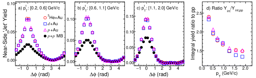
Figure 5: Estimated yield of near-side jet-like correlations for different trigger $p_{\mathrm{T}}$ values in MB $p$$+$$p$ and the top 0–10% of $p$$+$Au, $d$$+$Au, and ³He$+$Au collisions at $\sqrt{s_{{}_{\mathrm{NN}}}}=200$ GeV, distributed across three $p_{\mathrm{T}}^{\mathrm{t}}$ ranges in panels a), b), and c), respectively. In panel d), the ratios of yield between $p$/$d$/³He+Au and MB $p$$+$$p$, $Y_{\mathrm{int}}/Y_{\mathrm{int},pp}$, are demonstrated as a function of trigger $p_{\mathrm{T}}$. Associated particles are selected from $0.2<p_{\mathrm{T}}^{\mathrm{a}}<2$ GeV/$c$.

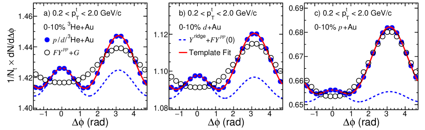
Figure 6: Performance assessment of the template-fit method for triggers within 0.2$<p_{\mathrm{T}}<$2.0 GeV/$c$ in the top 0–10% of $p$$+$Au, $d$$+$Au, and ³He$+$Au collisions at $\sqrt{s_{{}_{\mathrm{NN}}}}=200$ GeV. This assessment includes the ridge yield ($Y(\Delta\phi)^{\mathrm{ridge}}$) and the scaled yield of $p$$+$$p$ collisions ($Y(\Delta\phi)^{pp}$) multiplied by a factor of $F$. The coefficient $G$ represents the integrated yield of $Y(\Delta\phi)^{\mathrm{ridge}}$. Further details can be found in Eq. 14, Eq. 15, and the accompanying text.

In the $c_{0}$ method, non-flow effects in $p$/$d$/³He+Au collisions are assumed to arise from a convolution of several independent $p$$+$$p$ collisions. Consequently, they are expected to be proportional to $c_{n}^{pp}$, which is further divided by the $c_{0}$. The Fourier coefficients after subtracting non-flow contributions are calculated as follows:

$$c_{n}^{\mathrm{sub}}=c_{n}-\frac{c_{0}^{pp}}{c_{0}}\times c_{n}^{pp}\;.$$ (10)

This method is analogous to the “scalar-product method” mentioned in Refs. Adams et al. (2004) and Adams et al. (2005).

However, the $c_{0}$ method can underestimate non-flow contributions in central $p$/$d$/³He+Au collisions due to the selection of high-multiplicity events potentially biasing jet fragmentation to produce more correlated particle pairs. The near-side subtraction method from Refs. Adams et al. (2005); Aad et al. (2014); Adare et al. (2018) addresses this bias.

In the near-side subtraction method, the differences in non-flow contributions between $p$$+$$p$ and $p$/$d$/³He+Au collisions are estimated using the near-side per-trigger yield, $Y^{\mathrm{N}}(\Delta\phi)$, defined as the difference between the short-range yield integrated over $0.2<|\Delta\eta|<0.5$, denoted as $Y^{\mathrm{S}}(\Delta\phi)$, and the long-range yield integrated over $1.0<|\Delta\eta|<1.8$, denoted as $Y^{\mathrm{L}}(\Delta\phi)$. This method is illustrated by the equation,

$$Y_{\mathrm{int}}\equiv\int\!{Y^{\mathrm{N}}d\mbox{$\Delta\phi$}}=\!\int\!{(Y^{\mathrm{S}}-fY^{\mathrm{L}})d\mbox{$\Delta\phi$}}\;,$$ (11)

where $f=\frac{Y^{\mathrm{S}}(\mbox{$\Delta\phi$}=\pi)}{Y^{\mathrm{L}}(\mbox{$\Delta\phi$}=\pi)}$. The Fourier coefficients after subtracting non-flow contributions are obtained as,

$$c_{n}^{\mathrm{sub}}=c_{n}-\frac{Y_{\mathrm{int}}}{Y_{\mathrm{int},pp}}\frac{c_{0}^{pp}}{c_{0}}\times c_{n}^{pp},$$ (12)

The $Y^{\mathrm{N}}(\Delta\phi)$ distributions for various trigger particle $p_{\mathrm{T}}$ ranges are depicted in Fig. 5, and the ratio $Y_{\mathrm{int}}/Y_{\mathrm{int},pp}$ is shown in the right panel of the same figure. This ratio starts around 2.4 at low $p_{\mathrm{T}}$ and decreases rapidly with $p_{\mathrm{T}}$ while staying above unity. This indicates that the near-side subtraction method, compared to the $c_{0}$ method, removes a much larger portion of $p$$+$$p$-scaled correlations attributed to non-flow.

In the so-called $c_{1}$ method, non-flow contributions are directly estimated from the away-side jet-like correlations. In this method, the away-side jet contribution is assumed to scale with the $c_{1}$ component from the Fourier decomposition of $Y(\Delta\phi)$. This assumption holds at low $p_{\mathrm{T}}$, where the away-side jet shape is well described by a $1+2c_{1}\cos(\Delta\phi)$ function. However, we find that it is also a valid assumption over the entire $p_{\mathrm{T}}$ range considered in this analysis. In this context, the ratio of the non-flow component between $p$$+$$p$ and $p$/$d$/³He+Au is expected to be captured by the ratio of their respective $c_{1}$ values Adare et al. (2018). The non-flow subtracted Fourier coefficients are then calculated as,

$$c_{n}^{\mathrm{sub}}=c_{n}-\frac{c_{1}}{c_{1}^{pp}}\times c_{n}^{pp}\;.$$ (13)

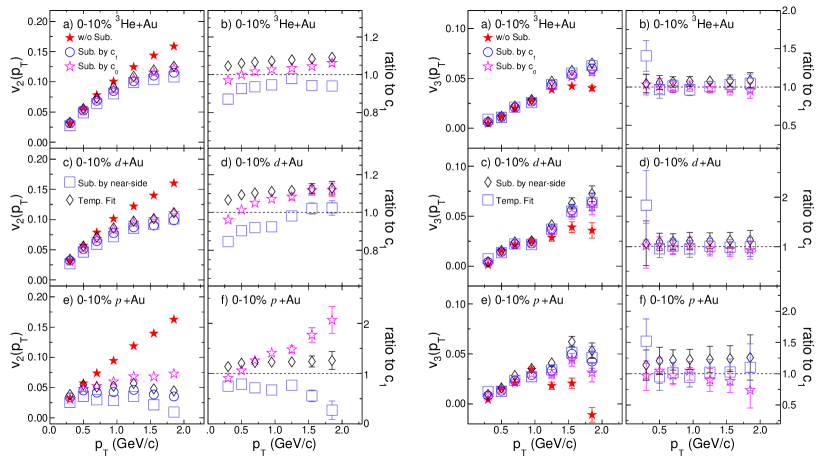
Figure 7: The $v_{2}(p_{\mathrm{T}})$ values (left figure) and $v_{3}(p_{\mathrm{T}})$ values (right figure) derived from different non-flow subtraction methods (left column) along with the ratios compared to those obtained through the $c_{1}$ method (right column) in the 0–10% most central $p$$+$Au, $d$$+$Au, and ³He$+$Au collisions. Only statistical uncertainties are depicted.

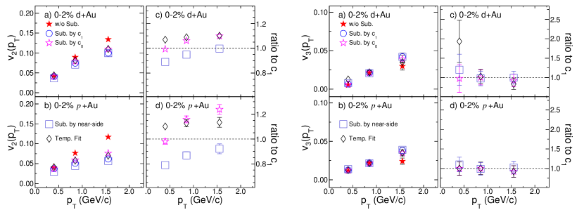
Figure 8: The $v_{2}(p_{\mathrm{T}})$ values (left figure) and $v_{3}(p_{\mathrm{T}})$ values (right figure) derived from different non-flow subtraction methods (left column) along with the ratios compared to those obtained through the $c_{1}$ method (right column) in the 0–2% most central $p$$+$Au and $d$$+$Au collisions. Only statistical uncertainties are depicted.

The last non-flow subtraction method implemented in this paper is the so-called “template-fit” method, developed by the ATLAS Collaboration and detailed in Ref. Aad et al. (2016). This method assumes that the $Y(\Delta\phi)$ in $p$/$d$/³He+Au collisions is a linear combination of a scaled $Y(\Delta\phi)$ distribution from MB $p$$+$$p$ collisions, representing all non-flow contributions, and a $Y(\Delta\phi)$ distribution containing only genuine collective flow, denoted as $Y(\Delta\phi)^{\mathrm{ridge}}$ ,

$$Y(\Delta\phi)^{\mathrm{templ}}=FY(\Delta\phi)^{pp}+Y(\Delta\phi)^{\mathrm{ridge}}\,,$$ (14)

where

$$Y(\Delta\phi)^{\mathrm{ridge}}=G\left(1+2\sum_{n=2}^{4}\ c_{n}^{\mathrm{sub}}\cos{(n\Delta\phi)}\right)\,.$$ (15)

The parameters $F$ and $c_{n}^{\mathrm{sub}}$ are determined through fitting the data to $Y(\Delta\phi)^{\mathrm{templ}}$. The coefficient $G$, determining the magnitude of the pedestal of $Y(\Delta\phi)^{\mathrm{ridge}}$, is fixed by ensuring that the integral of $Y(\Delta\phi)^{\mathrm{templ}}$ to equal to the integral of $Y(\Delta\phi)$ .

The performance of the template-fit method is shown in Fig. 6. The narrowing of the away-side peak in $p$/$d$/³He+Au collisions compared to that in $p$$+$$p$ collisions is a unique feature indicating the presence of a significant $\cos(2\Delta\phi)$ component Aad et al. (2016).

Since both the $c_{1}$ method and the template-fit method rely on the away-side jet correlation to constrain non-flow contributions, the scale factors in Eqs. 13 and 14 are expected to be similar, i.e., $F\approx c_{1}/c_{1}^{pp}$. The primary distinction between these methods lies in how they handle flow modulation. The $c_{1}$ method assumes that flow modulation affects all particle pairs, as captured by the $c_{0}$ term in Eq. 9, whereas the template-fit method assumes that flow modulation applies only to the subtracted pedestal, as represented by the parameter $G$ in Eq. 15. This implies that in central $p$/$d$/³He$+$Au collisions, where the particle multiplicity is much larger than that in $p$$+$$p$ collisions, the template-fit method is almost identical to the $c_{1}$ subtraction method.

The scale factors obtained from the four non-flow subtraction methods, as given by Eqs. 10, 12, 13, and 14, follow a consistent ordering: $\frac{c_{0}^{pp}}{c_{0}}<F\approx\frac{c_{1}}{c_{1}^{pp}}<\frac{Y_{\mathrm{int}}}{Y_{\mathrm{int},pp}}\frac{c_{0}^{pp}}{c_{0}}$. This indicates that the results obtained from the $c_{1}$ method and the template-fit method lie between those obtained from the $c_{0}$ method and the near-side subtraction method.

The difference in scale factors arises from the biases associated with jet fragmentation on the near side and the away side, which varies across the four subtraction methods. In two-particle correlations, pairs within the near-side jet peak require two particles originating from the same jet, while pairs within the away-side jet peak only need one particle each from the near-side and away-side jets. As a result, the near-side subtraction method tends to overestimate the non-flow contribution due to a larger jet fragmentation bias on the near-side jet. Conversely, the $c_{0}$ method tends to underestimate the non-flow contribution. Based on this analysis, the $c_{1}$ method is chosen as the default method in this study.

Note that the MB $p$$+$$p$ events used for non-flow estimation is biased by the trigger efficiency towards events with somewhat higher multiplicity. However, assuming that the shape of non-flow contribution in the correlation function is not modified, the trigger inefficiency in $p$$+$$p$ collisions is expected to not influence the subtraction procedure.

Finally, the flow coefficients $v_{n}$ are calculated using the two-particle harmonics $c_{n}(p_{\mathrm{T}}^{\mathrm{t}},p_{\mathrm{T}}^{\mathrm{a}})$ with or without non-flow subtractions,

$$v_{n}(p_{\mathrm{T}}^{\mathrm{t}})=\frac{c_{n}(p_{\mathrm{T}}^{\mathrm{t}},p_{\mathrm{T}}^{\mathrm{a}})}{\sqrt{c_{n}(p_{\mathrm{T}}^{\mathrm{a}},p_{\mathrm{T}}^{\mathrm{a}})}}\;,$$ (16)

By default, particle pairs are required to have a pseudorapidity gap of $|\mbox{$\Delta\eta$}|>1$, and the associated particles are chosen to have $0.2<p_{\mathrm{T}}^{\mathrm{a}}<2$ GeV/$c$.

The left part of Fig. 7 illustrates the extracted $v_{2}(p_{\mathrm{T}})$ in 0–10% central $p$$+$Au, $d$$+$Au, and ³He$+$Au collisions using different non-flow subtraction methods. The results agree with those before non-flow subtraction in the low $p_{\mathrm{T}}$ region ($<0.6$ GeV/$c$), but they are systematically smaller at higher $p_{\mathrm{T}}$. This behavior is consistent with the non-flow correlation from the away-side jet, which is expected to contribute more in smaller collision systems and at higher $p_{\mathrm{T}}$.

Among the four non-flow subtraction methods, the $v_{2}(p_{\mathrm{T}})$ values are in agreement within 20% in $d$$+$Au and ³He$+$Au collisions. In contrast, in $p$$+$Au collisions, the $v_{2}(p_{\mathrm{T}})$ values are similar at $p_{\mathrm{T}}<0.6$ GeV/$c$, but they exhibit a noticeable spread at higher $p_{\mathrm{T}}$. This observation suggests that $v_{2}(p_{\mathrm{T}})$ values can be extracted up to 2 GeV/$c$ in $d$$+$Au and ³He$+$Au, but only up to 0.6 GeV/$c$ in $p$$+$Au collisions.

The right part of Fig. 7 presents the same comparison for $v_{3}(p_{\mathrm{T}})$. The results after non-flow subtraction closely resemble those obtained without non-flow subtraction up to 1 GeV/$c$, but they are slightly larger at higher $p_{\mathrm{T}}$. The overall impact of non-flow correlations on $v_{3}(p_{\mathrm{T}})$ is significantly smaller than that on $v_{2}(p_{\mathrm{T}})$, resulting in a much weaker dependence of the extracted $v_{3}(p_{\mathrm{T}})$ values on the non-flow subtraction methods. This is because the away-side jet correlation centered around $\Delta\phi\sim\pi$ is very broad within the considered $p_{\mathrm{T}}^{\mathrm{a}},p_{\mathrm{T}}^{\mathrm{t}}$ range. Its Fourier decomposition gives rise to large negative $c_{1}$, a smaller positive $c_{2}$, and a much smaller negative $c_{3}$. The negative non-flow contribution to $c_{3}$ naturally implies that the non-flow subtraction procedure can only increase $v_{3}$, which is observed in Fig. 7. The spreads of $v_{3}(p_{\mathrm{T}})$ from different non-flow subtraction methods are approximately 10% in $d$$+$Au and ³He$+$Au, increasing to 20–30% in $p$$+$Au collisions.

The same analysis was also conducted for the 0–2% ultracentral $p$/$d$+Au collisions, and the results are depicted in Fig. 8. The dependence on the non-flow subtraction methods is qualitatively similar for both $v_{2}$ and $v_{3}$, although quantitatively, the variations in $p$$+$Au collisions are significantly reduced compared to Fig. 7. This reduction can be attributed to the higher $\langle N_{\mathrm{ch}}\rangle$ values in the 0–2% centrality range, as listed in Table 2, compared to the 0–10% centrality range in $p$$+$Au collisions. A larger $\langle N_{\mathrm{ch}}\rangle$ implies a significant decrease in the scale factors in all the non-flow subtraction methods, such as $c_{0}^{pp}/c_{0}$ in the $c_{0}$ and near-side subtraction methods, $c_{1}/c_{1}^{pp}$ in the $c_{1}$ method, and the $F$ in the template-fit method. This reduction in the scale factors diminishes the sensitivity to non-flow correlations and leads to smaller variations among different non-flow subtraction methods. This effect is most significant in $p$$+$Au collisions, but is less pronounced in $d$$+$Au collisions.

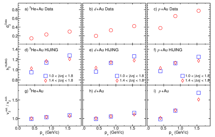
Figure 9: The values of $d_{2}\equiv\frac{c_{2}^{pp}}{c_{2}}\frac{c_{1}}{c_{1}^{pp}}$ calculated from real data with $|\Delta\eta|>1$ (top row), $h_{2}\equiv\frac{c_{2}^{pp\mathrm{hij}}}{c_{2}^{\mathrm{hij}}}\frac{c_{1}}{c_{1}^{pp}}$ derived from the HIJING model for two ranges of $|\Delta\eta|$ (middle row), and $v_{2}^{\text{est. }}/v_{2}^{\text{sub }}$ defined in Eq. 21 displayed as a function of $p_{\mathrm{T}}$ in central ³He$+$Au (left column), $d$$+$Au (middle column), and $p$$+$Au (right column) collisions. Only statistical uncertainties are shown.

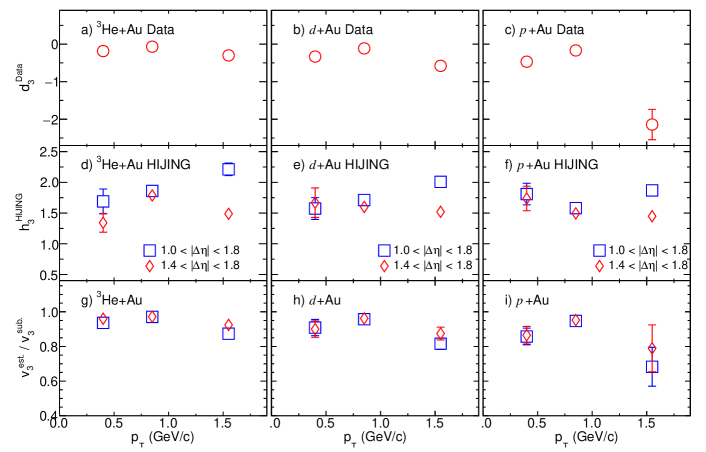
Figure 10: The values of $d_{3}\equiv\frac{c_{3}^{pp}}{c_{3}}\frac{c_{1}}{c_{1}^{pp}}$ calculated from real data with $|\Delta\eta|>1$ (top row), $h_{3}\equiv\frac{c_{3}^{pp\mathrm{hij}}}{c_{3}^{\mathrm{hij}}}\frac{c_{1}}{c_{1}^{pp}}$ derived from the HIJING model for two ranges of $|\Delta\eta|$ (middle row), and $v_{3}^{\text{est. }}/v_{3}^{\text{sub}}$ defined in Eq. 21 displayed as a function of $p_{\mathrm{T}}$ in central ³He$+$Au (left column), $d$$+$Au (middle column), and $p$$+$Au (right column) collisions. Only statistical uncertainties are shown.

III.3 Closure test of the non-flow subtraction with HIJING

In this section, a closure test of the non-flow subtraction method with the HIJING model is presented. This test aims to assess the validity of the non-flow subtraction procedures by comparing the results obtained from data with those from the HIJING model, which only includes non-flow correlations.

As discussed in the previous section, various non-flow subtraction methods differ mainly in estimating the scale factor $K$ to be multiplied to the $p$$+$$p$ Fourier harmonics,

$$c^{\mathrm{sub}}_{n}=c_{n}-K\times{c^{pp}_{n}}\;,$$ (17)

where $K$ is equal to $c_{0}^{pp}/c_{0}$ for the $c_{0}$ method and $c_{1}/c_{1}^{pp}$ for the $c_{1}$ method. However, for the following discussion, we will focus on the default $c_{1}$ method.

One may estimate the residual non-flow as the $c^{\mathrm{sub}}_{n}$ calculated directly using models such as HIJING Khachatryan et al. (2010); Lim et al. (2019). However, this approach relies on the model to reproduce the main features of jet-like correlations in $pp$ collisions, such as its $\Delta\phi$, $\Delta\eta$, and $p_{\mathrm{T}}$ dependence, which is not the case. Here, we take a different approach. In our approach, the features of non-flow are taken directly from $pp$ data, but only the difference of the factor $K$ in Eq. 17 between HIJING model and data is used to perform the closure test. The advantage is that we only rely on the HIJING model to estimate the scaling behavior of non-flow as a function of $\left\langle N_{\mathrm{ch}}\right\rangle$ and between different collision systems, not its absolute yield.

The factor $K$ in Eq. 17 could potentially be overestimated or underestimated by a factor $h_{n}$ that depends on the harmonic number $n$. However, $h_{n}$ cannot be directly determined from experimental data but can be explored using the HIJING model, where $h_{n}$ can be calculated by scaling the Fourier harmonics in $p$$+$$p$ collisions to match those in $p/d/^{3}$He+Au collisions:

$$c_{n}^{\mathrm{sub,hij}}=c_{n}^{\mathrm{hij}}-\frac{K}{h_{n}}\times{c^{pp,\mathrm{hij}}_{n}}=0\rightarrow h_{n}=K\frac{c^{pp,\mathrm{hij}}_{n}}{c_{n}^{\mathrm{hij}}}\;.$$ (18)

Here, $c^{pp,\mathrm{hij}}_{n}$ and $c_{n}^{\mathrm{hij}}$ represent the corresponding Fourier harmonics in HIJING simulations. It’s noted that $h_{n}$ is always positive, as both $c^{pp}_{n}$ and $c_{n}$ are positive quantities in the HIJING model.

We need to consider two scenarios for $h_{n}$, with respect to its harmonic number,

• For $n=2$, since $c^{pp}_{2}$ in Eq. 17 is positive, $h_{2}>1$ ($h_{2}<1$) would indicate overestimation (underestimation) of non-flow contributions for elliptic flow measurements.

• For $n=3$, since $c^{pp}_{3}<0$, $h_{3}<1$ ($h_{3}>1$) would imply overestimation (underestimation) of non-flow contributions for triangular flow measurements.

These scenarios lead to different impacts of non-flow subtractions on $v_{2}$ and $v_{3}$ in the context of the HIJING model.

In the framework of the closure test, the degree to which the $c_{1}$ method accurately characterizes non-flow correlations can be assessed using the following equation,

$$\frac{c^{\mathrm{est.}}_{n}}{c^{\mathrm{sub}}_{n}}=\frac{c_{n}-(K/h_{n})\times{c^{pp}_{n}}}{c_{n}-K\times{c^{pp}_{n}}}=\frac{1-d_{n}/h_{n}}{1-d_{n}}\;,$$ (19)

where $c^{\mathrm{est.}}_{n}$ represents the two-particle flow coefficients calculated using the scale factor obtained from the HIJING simulation. This value deviates from $c^{\mathrm{sub}}_{n}$ if and only if $h_{n}\neq 1$. In addition, we also define a new quantity $d_{n}$ based on real data,

$$d_{n}=K\frac{c^{pp}_{n}}{c_{n}}\;,$$ (20)

whose form is similar to $h_{n}$ in Eq. 18, although with different behavior in terms of its sign. Specifically, we expect that

• $d_{2}$ is always positive since both $c^{pp}_{2}$ and $c_{2}$ in the data are positive.

• $d_{3}$ is always negative due to the fact that $c^{pp}_{3}<0$ and $c_{3}>0$ in the data.

This distinction leads to a redefinition of Eq. 19 for the two harmonics, yielding an estimate of the potential change in $v_{n}$ due to non-flow subtraction uncertainties,

$$\frac{v^{\mathrm{est.}}_{2}}{v^{\mathrm{sub}}_{2}}\approx\frac{c^{\mathrm{est.}}_{2}}{c^{\mathrm{sub}}_{2}}=\frac{1-|d_{2}|/h_{2}}{1-|d_{2}|},$$ (21)

$$\frac{v^{\mathrm{est.}}_{3}}{v^{\mathrm{sub}}_{3}}\approx\frac{c^{\mathrm{est.}}_{3}}{c^{\mathrm{sub}}_{3}}=\frac{1+|d_{3}|/h_{3}}{1+|d_{3}|},$$ (22)

where we have used the factorization assumption and the observation that $v^{\mathrm{est.a}}_{2}/v^{\mathrm{sub,a}}_{2}\approx 1$, i.e. flow at low $p_{\mathrm{T}}$, covered by associated particles, is insensitive to the non-flow subtraction procedure,

$$\frac{c^{\mathrm{est.}}_{n}}{c^{\mathrm{sub}}_{n}}=\frac{v^{\mathrm{est.t}}_{n}}{v^{\mathrm{sub,t}}_{n}}\frac{v^{\mathrm{est.a}}_{n}}{v^{\mathrm{sub,a}}_{n}}\approx\frac{v^{\mathrm{est.t}}_{n}}{v^{\mathrm{sub,t}}_{n}}$$ (23)

Considering the differing signs between Eq. 21 and Eq. 22, it is expected that, for the same $h_{n}$ and $|d_{n}|$ values, $\frac{v_{3}^{\text{est. }}}{v_{3}^{\text{subl }}}$ would be closer to unity than $\frac{v_{2}^{\text{est. }}}{v_{2}^{\text{sub }}}$. Consequently, we anticipate that $v_{3}$ would be more robust, compared to $v_{2}$, against uncertainties associated with non-flow subtraction.

In Fig. 9, the outcomes of $d_{2}$ from data, $h_{2}$ from HIJING, and the resulting $v_{2}^{\text{est. }}/v_{2}^{\text{sub }}$ are displayed as functions of $p_{\mathrm{T}}$ for the three small collision systems. The top row presents the calculated $d_{2}$ using $|\Delta\eta|>1$. The upward trend with increasing $p_{\mathrm{T}}$ in $d_{2}$ reflects the larger non-flow contribution from the away-side jet. Notably, in $p$$+$Au collisions, $d_{2}$ reaches a value of 0.6–0.8 at high $p_{\mathrm{T}}$, indicating a significant reduction in the denominator of Eq. 21 and an enhanced sensitivity to the systematic uncertainties of non-flow subtraction.

In the middle row, $h_{2}$ from HIJING is plotted as a function of $p_{\mathrm{T}}$ for the three systems. The simulation indicates that the correlation functions in HIJING tend to exhibit broader near-side peaks compared to the data (as seen in Fig. 25 in Appendix VIII). Consequently, even after applying the $|\Delta\eta|>1$ cut, the residual near-side jet in the HIJING model may still bias the estimated $h_{2}$ value more than in the data. When applying a stricter cut of $|\Delta\eta|>1.4$, the shape of the correlation functions in Fig. 25 looks much more similar to the data. Nevertheless, we calculate $h_{2}$ from both $|\mbox{$\Delta\eta$}|>1$ and $|\mbox{$\Delta\eta$}|>1.4$ cuts, whose values are fortuitously similar. The values of $h_{2}$ are always above unity: they increase with $p_{\mathrm{T}}$, but are quite similar in the three systems.

The bottom row of Fig. 9 presents the results of $v_{2}^{\text{est.}}/v_{2}^{\text{sub }}$. Given that $h_{2}>0$, the nonflow scale factors obtained from HIJING are smaller than those derived from the data, resulting in larger $v_{2}$ values. If the HIJING model indeed provides accurate scale factors, these results would suggest that the $c_{1}$ method tends to overcorrect the $v_{2}$ values in the data. The degree of overcorrection amounts to approximately 0–8% in ³He$+$Au, 0–15% in $d$$+$Au, and 0–50% in $p$$+$Au collisions, across the measured $p_{\mathrm{T}}$ range.

In Fig. 10, the results of $d_{3}$ from data and $h_{3}$ from HIJING are displayed, alongside the corresponding $v_{3}^{\text{est. }}/v_{3}^{\text{sub }}$ as functions of $p_{\mathrm{T}}$ for the three collision systems. The top row shows the calculated $d_{3}$ values, which are consistently negative as anticipated. Moreover, the magnitude of $d_{3}$ increases with increasing $p_{\mathrm{T}}$.

The middle row of the figure presents $h_{3}$ from HIJING as a function of $p_{\mathrm{T}}$ for the three systems. Notably, $h_{3}$ values in all three systems are above unity, ranging from around 1.5–2.0, and exhibit only weak dependence on $p_{\mathrm{T}}$. This finding implies that the numerator in Eq. 22 is smaller than the denominator, indicating that $v_{3}^{\text{est. }}<v_{3}^{\text{sub }}$. This observation is consistent with the results shown in the bottom row, where the estimated flow signal after accounting for non-flow from HIJING is consistently smaller than the measurement. Specifically, $v_{3}^{\text{est. }}$ is smaller than $v_{3}^{\text{sub }}$ by approximately 5–10 % in ³He$+$Au, 10–15% in $d$$+$Au, and 15–20 % in $p$$+$Au collisions. This indicates that the $c_{1}$ method could overestimate the $v_{3}$ signal in the data by these magnitudes in a $p_{\mathrm{T}}$-independent manner, assuming that the non-flow correlations are correctly described by the HIJING model.

To sum up, the scaling behavior of non-flow in the HIJING model shows some differences from the real data. If the scale factors from HIJING are utilized to adjust the non-flow subtraction procedure, the $v_{2}$ values remain largely consistent, except for $p$$+$Au collisions at high $p_{\mathrm{T}}$. On the other hand, the $v_{3}$ values would be slightly reduced by less than 4–25 % across all collision systems and $p_{\mathrm{T}}$ ranges.

A previous study in Ref. Lim et al. (2019) explored the performance of the nonflow subtraction procedure using the HIJING model. The study identified residual non-closure of the subtraction, although it was conducted within a somewhat different $p_{\mathrm{T}}$ range. The findings indicated that the non-closure effect is significant in $p$$+$Au collisions at high $p_{\mathrm{T}}$ ($>1$ GeV/$c$), which aligns with the observations made in this analysis.

It is important to note that, however, based on the analysis method and kinematic selection employed by STAR, the impact of this non-closure has only a modest effect on the $v_{3}$ results, and is well within the experimental systematic uncertainties (see Table 3).

III.4 The dependence on the $\Delta\eta$ selection

In this section, we delve into the effect of varying the pseudorapidity gap $(|\mbox{$\Delta\eta$}|)$ between particle pairs, aiming to further assess the resilience of the non-flow subtraction methods. The default criterion for this gap is $|\mbox{$\Delta\eta$}|>1.0$, which effectively mitigates the impact of near-side non-flow correlations and reduces the influence of away-side non-flow. The chosen default non-flow subtraction method is the $c_{1}$ approach, and our focus is on scrutinizing the stability of the resulting $v_{n}$ values when applying different $|\mbox{$\Delta\eta$}|$ cuts.

We systematically adjust the $|\mbox{$\Delta\eta$}|$ cut for particle pairs and investigate the $v_{2}$ and $v_{3}$ values both with and without non-flow subtraction. The obtained results are presented in Fig. 11 for $v_{2}$ and Fig. 12 for $v_{3}$. Through this analysis, we uncover insightful observations regarding the impact of non-flow correlations.

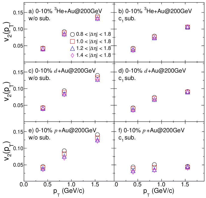
Figure 11: The values of $v_{2}$ obtained from distinct $\Delta\eta$ selections such as $|\Delta\eta|>$ 0.8, 1.0, 1.2 and 1.4 in top 0–10% $p$$+$Au, $d$$+$Au and ³He$+$Au collisions at $\sqrt{s_{{}_{\mathrm{NN}}}}=200$ GeV. The left column illustrates the results before non-flow subtraction, while the right column displays the results after applying the $c_{1}$ subtraction method. Only statistical uncertainties are shown.

Regarding $v_{2}$, the primary source of non-flow originates from the away-side jet-like correlations. By augmenting the $|\mbox{$\Delta\eta$}|$ cut from $|\mbox{$\Delta\eta$}|>0.8$ to $|\mbox{$\Delta\eta$}|>1.4$, the near-side residual non-flow is further suppressed; the overall non-flow contribution, however, experiences only a slight reduction with increasing $|\mbox{$\Delta\eta$}|$. This phenomenon clarifies the modest decline in $v_{2}$ seen in the left column of Fig. 11 before non-flow subtraction. This reduction becomes particularly conspicuous at $\approx 1.6$ GeV/$c$. Nevertheless, the $c_{1}$ subtraction methodology effectively eliminates most non-flow correlations, as shown in the right column of Fig. 11, yielding $v_{2}$ values that are smaller yet remain nearly independent of the $|\mbox{$\Delta\eta$}|$ cut.

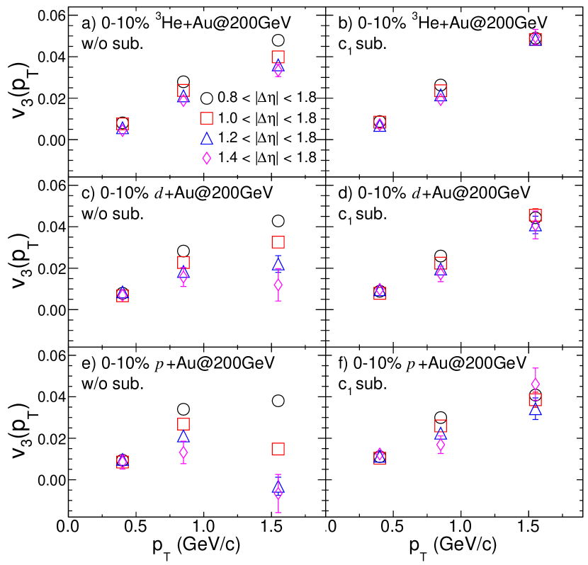
Figure 12: The values of $v_{3}$ obtained from distinct $\Delta\eta$ selections such as $|\Delta\eta|>$ 0.8, 1.0, 1.2 and 1.4 in top 0–10% $p$$+$Au, $d$$+$Au and ³He$+$Au collisions at $\sqrt{s_{{}_{\mathrm{NN}}}}=200$ GeV. The left column illustrates the results before non-flow subtraction, while the right column displays the results after applying the $c_{1}$ subtraction method. Only statistical uncertainties are shown.

The behavior of $v_{3}$ is more intricate. As mentioned previously, the away-side jet-like correlation tends to reduce the $v_{3}$. In contrast, any residual near-side jet correlations inherently lead to a positive $c_{3}$ value, thereby increasing the $v_{3}$ value. Consequently, the non-flow contributions stemming from both the near-side and away-side jets are in competition and can partly offset each other. This interplay is precisely what is observed in the left column of Fig. 12: increasing the $|\mbox{$\Delta\eta$}|$ cut curtails the positive contribution tied to the near-side jet, resulting in a reduction of the extracted $v_{3}$. This trend is evident across all three collision systems, with the most marked impact witnessed in $p$$+$Au collisions at high $p_{\mathrm{T}}$ (bottom-left panel of Fig. 12). Nevertheless, upon applying the non-flow subtraction, the $v_{3}$ values originating from very diverse $|\mbox{$\Delta\eta$}|$ cuts agree nicely with each other, as demonstrated in the right column of Fig. 12. This alignment implies that both the non-flow contributions affiliated with the near-side and away-side have been effectively eliminated.

It is pertinent to observe that the $v_{3}$ results for $|\mbox{$\Delta\eta$}|>0.8$ are nearly the same before and after non-flow subtraction. This suggests that the positive contribution linked to near-side jets and the negative contribution arising from away-side jets fortuitously offset each other.

In conclusion, this investigation suggests that adopting $|\mbox{$\Delta\eta$}|>1.0$ constitutes an optimal choice for the STAR TPC acceptance, as it strikes a balance between non-flow effects and statistical precision in the assessment of $v_{2}$ and $v_{3}$.

III.5 Non-flow bias in selecting high-multiplicity events

By default, the selection of centrality is based on the $N_{\mathrm{ch}}^{\mathrm{raw}}$ measured in the TPC (see Sec. II.2). This approach allows us to reach high values of $N_{\mathrm{ch}}^{\mathrm{raw}}$ for the flow measurement. However, this approach may cause potential bias on jet fragmentation, which in turn may bias the non-flow contributions. To explore the potential biases arising from the choice of high-multiplicity events on non-flow correlations, we carry out an analysis using two distinct centrality definitions, one relying on the TPC and the other on the multiplicity measured in the forward rapidity using $\Sigma Q_{\mathrm{BBCE}}$. A comparison between the $v_{n}$ values obtained from these two centrality definitions, using the $c_{0}$ and $c_{1}$ non-flow subtraction methods, is depicted in Figure 13.

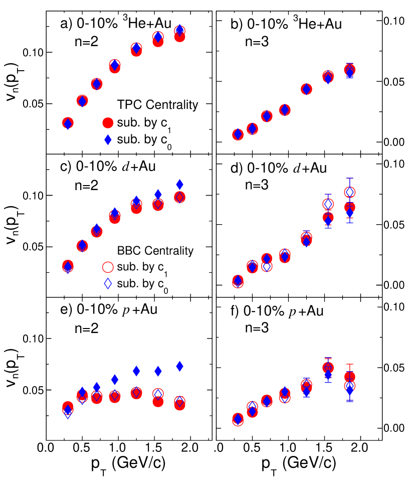
Figure 13: The $v_{2}$ values (left) and $v_{3}$ values (right) in central collisions based on TPC selection (filled symbols) and BBC selection (open symbols), obtained using the $c_{1}$ method (circles) and $c_{0}$ method (diamond) in 0–10% ³He$+$Au (top row), 0–10% $d$$+$Au (middle row) and 0–10% $p$$+$Au (bottom row) collisions. These results are obtained with a requirement of $|\Delta\eta|>1.0$. Only statistical uncertainties are displayed.

Firstly, we observe a high level of consistency between the two non-flow subtraction methods when adopting the BBC-based centrality selection. However, when employing the TPC-based centrality approach, the $v_{2}$ values exhibit notable differences between the two non-flow subtraction methods, particularly evident in $p$$+$Au collisions at high $p_{\mathrm{T}}$. These differences can be attributed to biases induced by the away-side non-flow on the per-trigger yield, which is underestimated by the scaling factor $c_{0}^{pp}/c_{0}$ employed in the $c_{0}$ method (Eq. 10). Conversely, the scale factor $c_{1}/c_{1}^{pp}$ utilized in the $c_{1}$ method (Eq. 12) accurately encapsulates the magnitude of the away-side non-flow, independent of the chosen centrality definition. This comparison strongly implies that the $c_{1}$ method is more reliable than the $c_{0}$ method in gauging the non-flow contribution.

Regarding $v_{3}$, the results are considerably less sensitive to the chosen centrality approach. This outcome is not surprising, given our demonstrations in previous sections that $v_{3}$ values are less susceptible to non-flow correlations under the kinematic criteria employed in this analysis.

Sources		$p_{\mathrm{T}}$ range(GeV/$c$)	0–10% 3He$+$Au	0–10% $d$$+$Au	0–10% $p$$+$Au	0–2% $d$$+$Au	0–2% $p$$+$Au
Track selection	$v_{2}$	0.2$<p_{\mathrm{T}}<$0.6	$<$ 2%	$<$ 2%	$<$ 5%	$<$ 2%	$<$ 2%
		0.6$<p_{\mathrm{T}}<$1.1	$<$ 2%	$<$ 2%	$<$ 5%	$<$ 2%	$<$ 2%
		1.1$<p_{\mathrm{T}}<$2.0	$<$ 2%	$<$ 2%	$<$ 5%	$<$ 2%	$<$ 2%
	$v_{3}$	0.2$<p_{\mathrm{T}}<$0.6	$<$ 2%	$<$ 6%	$<$ 4%	$<$ 6%	$<$ 10%
		0.6$<p_{\mathrm{T}}<$1.1	$<$ 2%	$<$ 5%	$<$ 9%	$<$ 5%	$<$ 9%
		1.1$<p_{\mathrm{T}}<$2.0	$<$ 2%	$<$ 4%	$<$ 3%	$<$ 4%	$<$ 3%
Matching to TOF/HFT	$v_{2}$	0.2$<p_{\mathrm{T}}<$0.6	$<$ 2%	$<$ 2%	$<$ 2%	$<$ 2%	$<$ 2%
		0.6$<p_{\mathrm{T}}<$1.1	$<$ 2%	$<$ 2%	$<$ 3%	$<$ 2%	$<$ 2%
		1.1$<p_{\mathrm{T}}<$2.0	$<$ 2%	$<$ 2%	$<$ 3%	$<$ 2%	$<$ 2%
	$v_{3}$	0.2$<p_{\mathrm{T}}<$0.6	$<$ 3%	$<$ 5%	$<$ 3%	$<$ 8%	$<$ 3%
		0.6$<p_{\mathrm{T}}<$1.1	$<$ 3%	$<$ 3%	$<$ 3%	$<$ 2%	$<$ 3%
		1.1$<p_{\mathrm{T}}<$2.0	$<$ 3%	$<$ 8%	$<$ 12%	$<$ 7%	$<$ 5%
Luminosity dependence	$v_{2}$	0.2$<p_{\mathrm{T}}<$2.0	$<$ 2%	$<$ 2%	$<$ 2%	$<$ 2%	$<$ 2%
	$v_{3}$	0.2$<p_{\mathrm{T}}<$2.0	$<$ 5%	$<$ 5%	$<$ 5%	$<$ 5%	$<$ 5%
Non-flow subtraction	$v_{2}$	0.2$<p_{\mathrm{T}}<$0.6	$<$ 13%	$<$ 15%	$<$ 28%	$<$ 15%	$<$ 29%
		0.6$<p_{\mathrm{T}}<$1.1	$<$ 8%	$<$ 11%	$<$ 34%	$<$ 9%	$<$ 16%
		1.1$<p_{\mathrm{T}}<$2.0	$<$ 9%	$<$ 12%	$<$ 64%	$<$ 10%	$<$ 24%
	$v_{3}$	0.2$<p_{\mathrm{T}}<$0.6	$<$18%	$<$ 21%	$<$ 29%	$<$6%	$<$ 27%
		0.6$<p_{\mathrm{T}}<$1.1	$<$ 17%	$<$ 21%	$<$ 34%	$<$ 12%	$<$ 26%
		1.1$<p_{\mathrm{T}}<$2.0	$<$ 8%	$<$ 12%	$<$ 24%	$<$ 17%	$<$ 13%
Total	$v_{2}$	0.2$<p_{\mathrm{T}}<$0.6	$<$ 13%	$<$ 16%	$<$ 29%	$<$ 16%	$<$ 25%
		0.6$<p_{\mathrm{T}}<$1.1	$<$ 9%	$<$ 12%	$<$ 34%	$<$ 9%	$<$ 16%
		1.1$<p_{\mathrm{T}}<$2.0	$<$ 9%	$<$ 13%	$<$ 65%	$<$ 10%	$<$ 24%
	$v_{3}$	0.2$<p_{\mathrm{T}}<$0.6	$<$ 19%	$<$ 21%	$<$ 30%	$<$ 13%	$<$ 29%
		0.6$<p_{\mathrm{T}}<$1.1	$<$ 19%	$<$ 22%	$<$ 34%	$<$ 14%	$<$ 28%
		1.1$<p_{\mathrm{T}}<$2.0	$<$ 11%	$<$ 13%	$<$ 28%	$<$ 19%	$<$ 15%

Table 3: Main sources of systematic uncertainties for $v_{2}$ and $v_{3}$ measurements in 0–10% central ³He$+$Au, $d$$+$Au and $p$$+$Au collisions and 0–2% ultracentral $d$$+$Au and $p$$+$Au collisions.

IV Systematic Uncertainties

The systematic uncertainties affecting $v_{n}$ measurements stem from various origins, encompassing track selection criteria, background tracks, residual pileup events, and non-flow subtraction procedures. For each variation, the entire analysis pipeline, including non-flow subtraction, is repeated, and the discrepancies from the default results are reported as uncertainties.

The influence of track selection is evaluated by modifying the TPC hit selection from 16 to 25 hits and by varying the DCA cut. The resultant changes remain below 5% for $v_{2}$ and below 10% for $v_{3}$ across all three collision systems. The criteria for matching tracks to fast detectors, crucial for background track elimination, are adjusted by requiring only TOF or either TOF or HFT in track matching. This adjustment induces deviations of less than 2% for $v_{2}$ and under 5% for $v_{3}$ in ³He$+$Au and $d$$+$Au collisions. In $p$$+$Au collisions, the variation spans 2% to 7% over $p_{\mathrm{T}}$ for $v_{2}$ and is under 5% for $v_{3}$.

The luminosity conditions differ notably among the $p$$+$$p$ and $p/d/^{3}$He+Au collisions. High luminosity running conditions can slightly diminish track reconstruction efficiency, which we counteract by implementing luminosity-dependent scaling factors integrated into the two-particle correlation analysis. However, varying luminosity may lead to fluctuations in track quality and background contamination. To address this, the data for each collision system is divided into subsets, each corresponding to distinct average luminosities measured by the STAR BBC. Subsequent correlation analyses are performed for each subset and compared. This analysis shows only minimal dependence on luminosity condition, resulting in a 2% uncertainty for $v_{2}$ and a 5% uncertainty for $v_{3}$ for all three systems.

Undoubtedly, the largest source of systematic uncertainty stems from our limited knowledge of non-flow contributions. Comprehensive discussions of non-flow subtraction methods and their efficacy have been provided in Section III. Here, we outline how uncertainty is quantified. The $v_{n}$ values are compared among four different subtraction methods and four distinct $\Delta\eta$ gaps ($|\Delta\eta|>$0.8, 1.0, 1.2, and 1.4). Further comparisons are made between correlations involving same-charge pairs and opposite-charge pairs. The differences between these two correlation functions allow us to assess the impact of residual contributions from near-side jet fragmentation.

Default results are obtained using the $c_{1}$ method with $|\Delta\eta|>$1.0, and the largest deviation from the other three subtraction methods is designated as the systematic uncertainty associated with the non-flow subtraction method. These uncertainties are then combined with variations among different $\Delta\eta$ gaps and those between same-charge and opposite-charge correlations. The uncertainty is under 15% (21%) for $v_{2}$($v_{3}$) in ³He$+$Au and $d$$+$Au collisions. For $p$$+$Au, the uncertainty is notably higher, reaching 65% for $v_{2}$ and 35% for $v_{3}$ at high $p_{\mathrm{T}}$. Notably, the uncertainties linked to non-flow subtraction methods are considerably smaller for the most central 0–2% $p$$+$Au collisions, compared to those for the 0–10% $p$$+$Au collisions.

The uncertainties originating from the aforementioned four different sources are combined in quadrature. Non-flow subtraction predominantly governs these uncertainties. The detailed breakdown of systematic uncertainties can be located in Table 3.

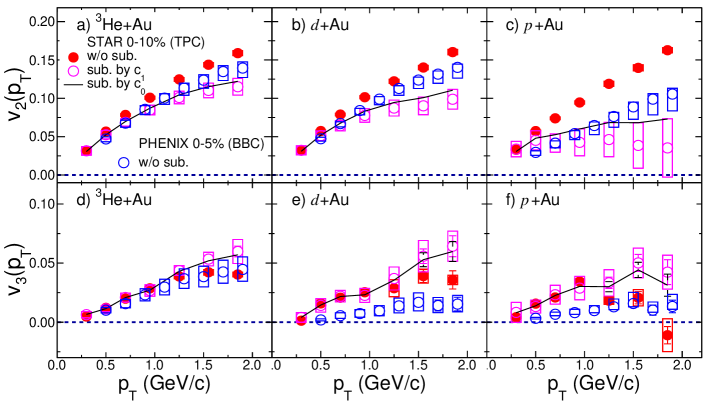
Figure 14: Comparison of the $v_{2}(p_{\mathrm{T}})$ (top row) and $v_{3}(p_{\mathrm{T}})$ (bottom row) between measurements obtained by PHENIX (open blue circles), STAR results without non-flow subtraction (solid red circles), as well as STAR results with non-flow subtraction based on $c_{1}$ method (pink open circles) and $c_{0}$ method (black lines). The boxes indicate the systematic uncertainties. The PHENIC results are obtained for 0–5% centrality. The STAR results are obtained for 0–10% centrality, whose systematic uncertainties are shown for without subtraction and with the $c_{1}$ subtraction method.

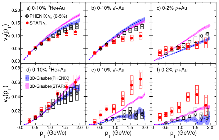
Figure 15: Comparison between the STAR results based on the $c_{1}$ method and PHENIX measurements, along with the 3D-Glauber calculations using middle-middle (STAR) or middle-backward (PHENIX) correlations. This comparison reveals a significant difference in $v_{3}(p_{\mathrm{T}})$ between the two experiments, which can be attributed to flow decorrelations, partially captured by the 3D-Glauber calculations Zhao et al. (2023). The boxes indicate the systematic uncertainties. Note that for $p$$+$Au collisions, the STAR results are shown for 0–2% centrality instead of the 0–10% in Fig. 14.

V Results and discussions

V.1 Comparison with previous results and model predictions

The flow results from the STAR and PHENIX experiments in small collision systems exhibit differences that can be attributed to various factors, including variations in kinematic selection, analysis techniques, residual non-flow correlations, and longitudinal dynamics. It is valuable to review these discrepancies for a comprehensive understanding.

The PHENIX measurements are obtained through multiple pairs of correlations involving different combinations of particles at midrapidity and in the backward Au-going direction: $|\eta^{a}|<$ 0.35, -3.0 $<\eta^{b}<$ -1.0, and -3.9 $<\eta^{c}<$ -3.1. Using the notation of flow vectors in a subevent as ${\bm{Q}}_{n}\equiv q_{n}e^{in\psi_{n}}$, the $v_{n}(p_{\mathrm{T}})$ at midrapidity ($|\eta^{a}|<$ 0.35) is computed using an event-plane method that assumes factorization among the pairs from any two subevents,

$$v_{n}^{a}(p_{\mathrm{T}})\approx\frac{\left\langle q_{n}^{a}(p_{\mathrm{T}})\cos n(\psi_{n}^{a}(p_{\mathrm{T}})-\psi_{n}^{c})\right\rangle\sqrt{\left\langle\cos n(\psi_{n}^{a}-\psi_{n}^{b})\right\rangle}}{\sqrt{\left\langle\cos n(\psi_{n}^{a}-\psi_{n}^{c})\right\rangle\left\langle\cos n(\psi_{n}^{c}-\psi_{n}^{b})\right\rangle}}\;,$$ (24)

where $q_{n}^{a}(p_{\mathrm{T}})$ and $\psi_{n}^{a}(p_{\mathrm{T}})$ denote the magnitude and direction (or event plane) of the flow vector ${\bm{Q}}_{n}(p_{\mathrm{T}})$ at midrapidity. The $\psi_{n}^{c}$ and $\psi_{n}^{b}$ are event planes calculated using all particles (without $p_{\mathrm{T}}$ selection) within the acceptance of a specific subevent.

In the low event plane resolution limit, this equation simplifies to the scalar product method result, which also incorporates $q_{n}$ as weights,

$$v_{n}^{a}(p_{\mathrm{T}}) =\!\frac{\left\langle q_{n}^{a}(p_{\mathrm{T}}\!)q_{n}^{c}\!\cos n(\!\psi_{n}^{a}(p_{\mathrm{T}}\!)\!-\!\psi_{n}^{c})\right\rangle\!\sqrt{\left\langle q_{n}^{a}q_{n}^{b}\cos n\!(\!\psi_{n}^{a}\!-\!\psi_{n}^{b})\right\rangle}}{\sqrt{\left\langle q_{n}^{a}q_{n}^{c}\cos n(\psi_{n}^{a}-\psi_{n}^{c})\right\rangle\left\langle q_{n}^{c}q_{n}^{b}\cos n(\psi_{n}^{c}-\psi_{n}^{b})\right\rangle}}$$

$$=\frac{\left\langle{\bm{Q}}_{n}^{a}(p_{\mathrm{T}}){\bm{Q}}_{n}^{c*}\right\rangle\sqrt{\left\langle{\bm{Q}}_{n}^{a}{\bm{Q}}_{n}^{b*}\right\rangle}}{\sqrt{\left\langle{\bm{Q}}_{n}^{a}{\bm{Q}}_{n}^{c*}\right\rangle\left\langle{\bm{Q}}_{n}^{c}{\bm{Q}}_{n}^{b*}\right\rangle}}$$ (25)

$$\equiv\frac{c_{n}(a(p_{\mathrm{T}}),c)\sqrt{{c_{n}(a,b)}}}{\sqrt{{c_{n}(a,c)}{c_{n}(c,b)}}}\;.$$ (26)

where, for instance, $c_{n}(c,b)$ represents the two-particle correlation for all particles accepted in subevents “$c$” and “$b$”. The $a(p_{\mathrm{T}})$ denotes that particles in subevent “$a$” are chosen from a certain $p_{\mathrm{T}}$ range.

In addition to Eq. 26, two independent combinations can also be used to calculate $v_{n}^{a}(p_{\mathrm{T}})$,

$$v_{n}^{a}(p_{\mathrm{T}}) =\sqrt{\frac{c_{n}(a(p_{\mathrm{T}}),c){c_{n}(a(p_{\mathrm{T}}),b)}}{c_{n}(c,b)}}$$

$$v_{n}^{a}(p_{\mathrm{T}}) =\frac{c_{n}(a(p_{\mathrm{T}}),b)\sqrt{{c_{n}(a,c)}}}{\sqrt{{c_{n}(a,b)}{c_{n}(c,b)}}}\;.$$ (27)

Assuming factorization relations such as ${c_{n}(a(p_{\mathrm{T}}),c)=v_{n}^{a}(p_{\mathrm{T}})v_{n}^{c}}$ and $c_{n}(c,b)=v_{n}^{c}v_{n}^{b}$, as often done in experimental measurements, it is evident that all three different combination reduces to the same $v_{n}^{a}(p_{\mathrm{T}})$. However, such factorization relations are explicitly broken by residual non-flow effects Liu et al. (2020) and longitudinal decorrelations Bozek and Broniowski (2016). Therefore, if these contributions are negligible, all three approaches are expected to yield equivalent results.

In contrast, the STAR measurements are derived from correlations between particles in the same mid-rapidity interval $|\eta^{a,b}|<$ 0.9 but with a definite pseudorapidity gap $|\mbox{$\Delta\eta$}|>1.0$ between the pairs, as defined in Eq. 16. This small pseudorapidity gap reduces the impact of longitudinal flow decorrelations, which could be prominent in smaller $p$$+$Au collisions Khachatryan et al. (2015).

In the PHENIX measurement, non-flow contributions are not subtracted from each of the $c_{n}$ terms in Eq. 26. Instead, these non-flow contributions are estimated using an approach similar to the $c_{0}$ subtraction method and are incorporated as asymmetric systematic uncertainties. On the other hand, we have demonstrated that the $c_{0}$ method, at least within the STAR acceptance, could underestimate non-flow and is also influenced by auto-correlation effects (Fig. 7 and Fig. 13). Therefore, the $c_{1}$ method is considered to be closer to the true flow value in this analysis.

Figure 14 provides a comparison of $v_{2}$ and $v_{3}$ results between the two experiments for similar $p_{\mathrm{T}}$ and centrality ranges. The STAR results, based on the $c_{1}$ and $c_{0}$ methods, are presented. The $v_{2}$ results without non-flow subtraction in ³He$+$Au and $d$$+$Au collisions are slightly higher than those of PHENIX, but they are 60% larger in $p$$+$Au collisions. This discrepancy reflects a greater non-flow contribution in the STAR measurements due to its smaller $\Delta\eta$ gap and larger away-side non-flow contributions. After non-flow subtraction, aside from minor $p_{\mathrm{T}}$-dependent differences for $p_{\mathrm{T}}>1$ GeV/$c$, where STAR results are systematically lower, the $v_{2}$ results are consistent between the two experiments within uncertainties.

As the asymmetric systematic uncertainties in PHENIX results account for non-flow estimates based on the $c_{0}$ method, it is insightful to compare them with STAR results obtained using the same method. Figure 14 reveals that the STAR $v_{2}$ values acquired from the $c_{0}$ method lie just below the lower limit of the uncertainty bands of the PHENIX results. In contrast, the STAR $v_{3}$ values computed using the $c_{0}$ method are noticeably outside the uncertainty region of corresponding PHENIX results. This discrepancy might partially stem from the effects of longitudinal decorrelations.

The recent calculations utilizing a 3D-Glauber model and discussed in the study by Zhao et al. Zhao et al. (2023) suggest that there is a more pronounced decorrelation effect in the flow measurement method adopted by PHENIX. As depicted in Fig. 15, this decorrelation could contribute about half of the difference in $v_{3}$ between the two experiments. On the other hand, this model underestimates $v_{3}$ measurements from both experiments in $p$$+$Au collisions.

In addition to residual non-flow correlations and longitudinal decorrelations affecting the two results differently, the measurements are also influenced by variations in modeling the initial collision geometry and early-time transverse dynamics, which are common to both experiments. These aspects are elaborated below.

Figure 16 contrasts the $v_{2}$ and $v_{3}$ results from the three systems with three hydrodynamic model calculations that make distinct assumptions about the initial collision geometry and early dynamics. The sonic model Romatschke (2015) incorporates viscous hydrodynamics with a nucleon Glauber initial geometry. The supersonic model from the same Ref. Romatschke (2015) introduces an additional pre-equilibrium flow phase, enhancing initial velocity fields during system evolution. The third model Schenke et al. (2020a, b) combines IP-Glasma initial conditions with subnucleon fluctuations and pre-flow effects, MUSIC for hydrodynamic evolution, and UrQMD for hadronic phase interactions. All three models’ initial conditions are boost invariant, meaning that both non-flow and longitudinal dynamics are absent. The transport coefficients in these models, such as shear viscosity and freeze-out conditions, have been tuned to describe flow data in large Au+Au collision systems.

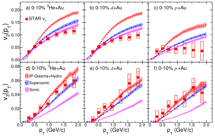
Figure 16: Comparison of $v_{2}(p_{\mathrm{T}})$ (top row) and $v_{3}(p_{\mathrm{T}})$ (bottom row) values based on the $c_{1}$ method in 0–10% most central ³He$+$Au (left column), $d$$+$Au (middle column), and $p$$+$Au (right column) collisions with calculations from three hydrodynamical models: the sonic model Romatschke (2015) (pink bands with dotted lines), the supersonic model (blue bands with dash-dotted lines) Romatschke (2015) and IP-Glasma+Hydro model (red bands with dashed lines) Schenke et al. (2020a, b). The boxes and shaded bands are the systematic uncertainties.

The comparison of these models with the experimental data yields interesting insights. The sonic model underestimates the $v_{3}$ values observed across all three collision systems. On the other hand, the supersonic model, which includes the pre-flow effect, achieves a better agreement with the experimental data. The IP-Glasma+hydro model manages to describe the $v_{3}$ results well in all three systems, but it tends to overestimate the $v_{2}$ results. This comparison underscores the complexity of interpreting small system flow data. To truly comprehend the roles played by pre-equilibrium flow, nucleon fluctuations, and subnucleon fluctuations in the initial conditions, comprehensive investigations are necessary. These studies should encompass further model refinements, the acquisition of additional small system collision data, and more differential measurements.

In this regard, STAR has collected new $d$$+$Au and ¹⁶O+¹⁶O data in 2021 using the updated detector systems. These upgrades include the inner TPC, which extends tracking to $|\eta|<$ 1.5 Wang et al. (2017), and the Event Plane Detector, capable of measuring charged particles in 2.1 $<|\eta|<$ 5.3 Adams et al. (2020). The utilization of this dataset will enable STAR to directly contrast correlations obtained at midrapidity with those between the middle and backward regions. This comparison holds the promise of shedding light on the roles of longitudinal decorrelation and non-flow correlations in small systems.

The symmetric ¹⁶O+¹⁶O system, which possesses a size, in terms of number of collided nucleons, similar to $d$$+$Au but markedly distinct geometry, is anticipated to be less influenced by subnucleon fluctuations and biases stemming from centrality selection. A comparison involving existing small system data at RHIC has the potential to untangle various competing effects related to initial geometry and hydrodynamic evolution. Furthermore, a comparison with future ¹⁶O+¹⁶O data at the LHC, scheduled for collection in 2024, will offer direct insights into the energy dependence of pre-flow and longitudinal dynamics. These future endeavors hold the key to a more comprehensive understanding of the intricate interplay between small system dynamics and the underlying physics mechanisms.

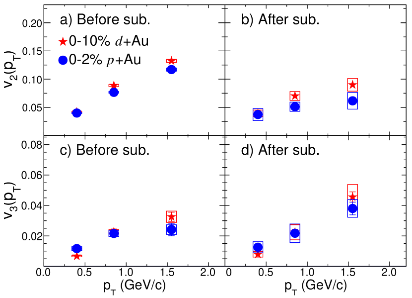
Figure 17: Comparison of $v_{2}(p_{\mathrm{T}})$ (top row) and $v_{3}(p_{\mathrm{T}})$ (bottom row) values based on the $c_{1}$ method in the 0–2% most central $p$$+$Au and 0–10% most central $d$$+$Au collisions before (left column) and after (right column) non-flow subtractions. The boxes and shaded bands are the systematic uncertainties.

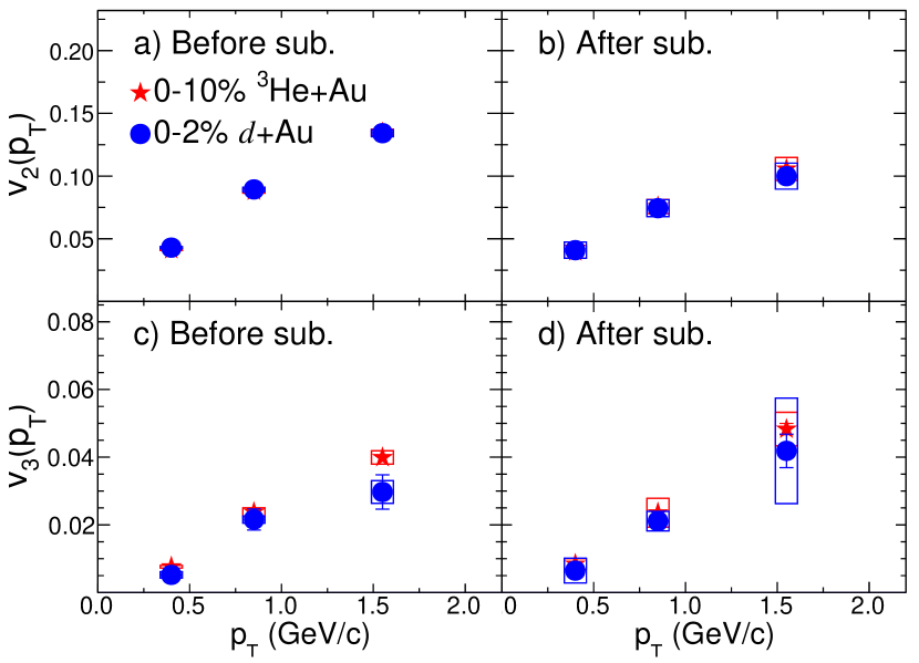
Figure 18: Comparison of $v_{2}(p_{\mathrm{T}})$ (top row) and $v_{3}(p_{\mathrm{T}})$ (bottom row) based on the $c_{1}$ method in the 0–2% most central $d$$+$Au and 0–10% most central ³He$+$Au collisions before (left column) and after (right column) non-flow subtractions. The boxes are the systematic uncertainties.

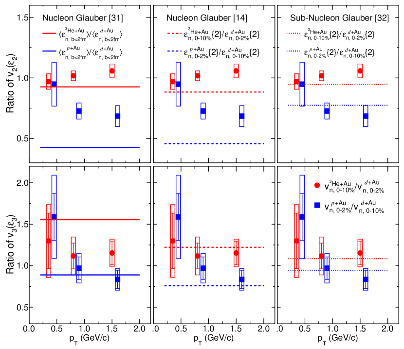
Figure 19: The ratios of $v_{2}(p_{\mathrm{T}})$ (top) and $v_{3}(p_{\mathrm{T}})$ (bottom) values obtained from the $c_{1}$ method between the 0–2% $p$$+$Au and 0–10% $d$$+$Au collisions (circles) and between the 0–2% $d$$+$Au and 0–10% ³He$+$Au collisions (squares). They are compared to ratios of $\varepsilon_{2}$ and $\varepsilon_{3}$ values from the Glauber models: nucleon Glauber model from Ref. Aidala et al. (2019) calculated with simple mean $\left\langle\varepsilon_{n}\right\rangle$ for $b<2$ fm (left column), nucleon Glauber model from Ref. Abdulhamid et al. (2023); Alver et al. (2008) calculated with $\varepsilon_{n}\{2\}\equiv\sqrt{\left\langle\varepsilon_{n}^{2}\right\rangle}$ (middle column) and quark Glauber model from Ref. Welsh et al. (2016) calculated with $\sqrt{\left\langle\varepsilon_{n}^{2}\right\rangle}$ (right column). The boxes are the systematic uncertainties.

V.2 Comparison of $v_{n}$ between different systems at similar multiplicity and constraining the initial geometry

An intriguing observation at the LHC is the similarity in magnitude and $p_{\mathrm{T}}$ dependencies of triangular flow in $p$+Pb and Pb+Pb collisions at the same overall multiplicity Khachatryan et al. (2017); Aad et al. (2014). This has given rise to the concept of conformal scaling Başar and Teaney (2014), which suggests that the ratios $v_{n}/\varepsilon_{n}$ should primarily depend on the charged particle multiplicity density ($dN_{\mathrm{ch}}/d\eta$). The underlying rationale is that the hydrodynamic response is controlled by the ratio of the mean free path to system size, which is essentially a power-law function of $dN_{\mathrm{ch}}/d\eta$ Başar and Teaney (2014). The validity of conformal scaling for $v_{n}$ is well-established in large collision systems, as evidenced by comparisons such as Au+Au and U+U Giacalone et al. (2021). Moreover, this scaling has proven effective for $v_{2}$ when considering average collision geometry in the comparison between $p$+Pb and Pb+Pb Başar and Teaney (2014), as well as for $v_{3}$ when accounting for possible oversubtraction of $v_{3}$ in $p$$+$$p$ collisions Aaboud et al. (2019). Assuming that $v_{n}$ is predominantly governed by final state effects, this line of reasoning motivates a similar universal scaling behavior in small systems at RHIC energy.

Considering two systems, A and B, with comparable charged particle multiplicities, we expect the following relation to hold,

$$\frac{v_{n}^{\rm A}}{v_{n}^{\rm B}}\approx\frac{\varepsilon_{n}^{\rm A}}{\varepsilon_{n}^{\rm B}}\;.$$ (28)

This relation implies that the ratio of $v_{n}$ between two systems largely cancels out most of the final state effects, thereby providing a means to constrain the ratio of their eccentricities.

Such comparative analysis can be carried out using the centrality selections outlined in Table 2. Notably, we find similar average charged particle multiplicities, $\left\langle N_{\mathrm{ch}}\right\rangle$, between the 0–2% $p$$+$Au and 0–10% $d$$+$Au systems, as well as between the 0–2% $d$$+$Au and 0–10% ³He$+$Au systems. The comparison between the 0–2% $p$$+$Au and 0–10% $d$$+$Au systems is presented in Fig. 17, while the comparison between the 0–2% $d$$+$Au and 0–10% ³He$+$Au systems is shown in Fig. 18.

The $v_{2}$ and $v_{3}$ results before and after non-flow subtraction exhibit remarkably similar behaviors for the 0–2% $d$$+$Au collisions and 0–10% centrality ³He$+$Au collisions. For the comparison between 0–2% $p$$+$Au and 0–10% $d$$+$Au collisions, $v_{3}$ values are similar, but there exists approximately a 20% difference in $v_{2}$.

To make the comparison more quantitative, we calculate the ratios of $v_{n}$ between 0–2% $p$$+$Au and 0–10% $d$$+$Au, as well as between 0–2% $d$$+$Au and 0–10% ³He$+$Au. These ratios are depicted in Fig. 19. The systematic uncertainties are largely correlated across different systems, including those arising from non-flow subtraction methods. The total uncertainties are approximately 5% for $v_{2}^{\scriptsize\mbox{${}^{3}$He$+$Au}}/v_{2}^{\scriptsize\mbox{$d$$+$Au}}$ and 10% to 20% for $v_{2}^{\scriptsize\mbox{$p$$+$Au}}/v_{2}^{\scriptsize\mbox{$d$$+$Au}}$. The uncertainties for the $v_{3}$ ratios are larger, particularly at the lowest $p_{\mathrm{T}}$ bin, but decrease to below 20% in the high $p_{\mathrm{T}}$ region. The ratio $v_{2}^{\scriptsize\mbox{$p$$+$Au}}/v_{2}^{\scriptsize\mbox{$d$$+$Au}}$ is approximately 20% below unity, indicating that $\varepsilon_{2}^{\scriptsize\mbox{$p$$+$Au}}$ is smaller than $\varepsilon_{2}^{\scriptsize\mbox{$d$$+$Au}}$ by a similar magnitude. In contrast, the $v_{3}$ ratios are close to unity, although the value of $v_{3}^{\scriptsize\mbox{${}^{3}$He$+$Au}}$ is systematically larger than $v_{3}^{\scriptsize\mbox{$d$$+$Au}}$ by about 10%, albeit within sizable uncertainties. This observation suggests that $\varepsilon_{3}$ in the three systems at similar multiplicities are roughly comparable.

A natural next step is to compare the ratios of $v_{n}$ to those of $\varepsilon_{n}$ from three Glauber model calculations. These calculations include fluctuations at nucleon level Nagle et al. (2014); Abdulhamid et al. (2023) or fluctuations at both nucleon and subnucleon level Welsh et al. (2016). Furthermore, the value of eccentricity depends on whether it is defined as simple mean $\left\langle\varepsilon_{n}\right\rangle$ Nagle et al. (2014) or root-mean-square $\varepsilon_{n}\{2\}\equiv\sqrt{\left\langle\varepsilon_{n}^{2}\right\rangle}$ Abdulhamid et al. (2023). The latter definition naturally yields larger values due to the inclusion of event-by-event fluctuations. This definition also shows smaller hierarchical differences between the three systems (see Table 1). However, since $v_{n}$ measured by the two-particle correlation method is effectively $\sqrt{\left\langle v_{n}^{2}\right\rangle}$, it seems that the $\varepsilon_{n}\{2\}$ is a more natural choice.

Figure 19 contrasts the ratios of $\varepsilon_{n}$ from these three Glauber models, calculated for the same centrality range. The two models without subnucleon fluctuations fail to reproduce the hierarchy of $v_{n}$ ratios indicated by the data. These models predict substantially smaller $\varepsilon_{2}$ values for $p$$+$Au than for $d$$+$Au collisions, as well as a greater $\varepsilon_{3}$ for ³He$+$Au than for $d$$+$Au collisions, a prediction at odds with the data. However, the model that defines eccentricity as its RMS value predicts a smaller difference between ³He$+$Au and $d$$+$Au.

On the other hand, the Glauber model that accounts for subnucleon fluctuations yields $\varepsilon_{2}$ and $\varepsilon_{3}$ ratios that align with the data. Notably, it validates the hypothesis of $\varepsilon_{3}^{\scriptsize\mbox{${}^{3}$He$+$Au}}/\varepsilon_{3}^{\scriptsize\mbox{$d$$+$Au}}>\varepsilon_{3}^{\scriptsize\mbox{$d$$+$Au}}/\varepsilon_{3}^{\scriptsize\mbox{$p$$+$Au}}\approx 1$, where $\varepsilon_{3}^{\scriptsize\mbox{${}^{3}$He$+$Au}}$ is found to be larger than $\varepsilon_{3}^{\scriptsize\mbox{$d$$+$Au}}$ by approximately 10%.

In summary, the Glauber model incorporating subnucleonic fluctuations exhibits an approximate hierarchy among the three systems,

$$\varepsilon_{2}^{\scriptsize\mbox{${}^{3}$He$+$Au}}\approx\varepsilon_{2}^{\scriptsize\mbox{$d$$+$Au}}>\varepsilon_{2}^{\scriptsize\mbox{$p$$+$Au}}\;,$$ (29)

$$\varepsilon_{3}^{\scriptsize\mbox{${}^{3}$He$+$Au}}\approx\varepsilon_{3}^{\scriptsize\mbox{$d$$+$Au}}\approx\varepsilon_{3}^{\scriptsize\mbox{$p$$+$Au}}\;.$$ (30)

consistent with those of the $v_{n}$.

VI Summary

We presented measurements of elliptic flow ($v_{2}$) and triangular flow ($v_{3}$) in high-multiplicity $p$/$d$/³He+Au collisions at $\sqrt{s_{\mathrm{NN}}}$ = 200 GeV. The measurements are performed using two-particle azimuthal angular correlations at mid-rapidity as a function of $p_{\mathrm{T}}$.

To correct for non-flow contributions, which arise from correlations not associated with collective flow, we estimate these contributions using minimum-bias $p$$+$$p$ collisions at the same energy and subtract them from the $p$/$d$/³He+Au collision results. We utilize four distinct state-of-the-art non-flow subtraction methods to quantify the uncertainties associated with the subtraction procedure. While we observe a notable impact of non-flow contributions on $v_{3}$ prior to subtraction, the $v_{3}$ values after subtraction exhibit consistency across different pseudorapidity gap selections. We also investigate the potential bias introduced by the selection of high-multiplicity events using alternative criteria. The result demonstrates overall agreement, except for $v_{2}$ in $p$$+$Au collisions for the $c_{0}$ subtraction methods. Furthermore, we perform a closure test of the non-flow subtraction procedure using simulations generated by the HIJING model. The level of closure is generally within the quoted systematic uncertainties, except for a few cases: $v_{2}$ results might be underestimated (oversubtracted) at high $p_{\mathrm{T}}$, particularly in $p$$+$Au collisions, while $v_{3}$ results could be slightly overestimated (undersubtracted) by approximately 10% across all systems and $p_{\mathrm{T}}$ ranges.

Notably, the systematic uncertainties of $v_{n}$ largely cancel out when forming ratios of $v_{n}$ in the three collision systems with comparable charged particle multiplicities. This observation supports a clear ordering of their magnitudes: $v_{2}^{\scriptsize\mbox{${}^{3}$He$+$Au}}\approx v_{2}^{\scriptsize\mbox{$d$$+$Au}}>v_{2}^{\scriptsize\mbox{$p$$+$Au}}$, and similarly, $v_{3}^{\scriptsize\mbox{${}^{3}$He$+$Au}}\approx v_{3}^{\scriptsize\mbox{$d$$+$Au}}\approx v_{3}^{\scriptsize\mbox{$p$$+$Au}}$. These orderings are in line with the ordering of eccentricities predicted by considering subnucleon fluctuations in the initial geometry.

However, the observed orderings are different from those observed by the PHENIX experiment, which measures correlations between particles at mid-rapidity and particles in the backward rapidity direction of the Au-going side. The observed orderings are more in line with the initial geometry that includes only nucleon fluctuations. A state-of-the-art hydrodynamic model analysis Zhao et al. (2023) suggests that this discrepancy could, in part, be attributed to longitudinal decorrelations of $v_{3}$ between mid-rapidity and backward rapidity. Additionally, models incorporating pre-equilibrium flow but lacking subnucleon fluctuations can also reproduce the measured $v_{3}$ values.

VII Acknowledgement

We thank the RHIC Operations Group and RCF at BNL, the NERSC Center at LBNL, and the Open Science Grid consortium for providing resources and support. This work was supported in part by the Office of Nuclear Physics within the U.S. DOE Office of Science, the U.S. National Science Foundation, National Natural Science Foundation of China, Chinese Academy of Science, the Ministry of Science and Technology of China and the Chinese Ministry of Education, the Higher Education Sprout Project by Ministry of Education at NCKU, the National Research Foundation of Korea, Czech Science Foundation and Ministry of Education, Youth and Sports of the Czech Republic, Hungarian National Research, Development and Innovation Office, New National Excellency Programme of the Hungarian Ministry of Human Capacities, Department of Atomic Energy and Department of Science and Technology of the Government of India, the National Science Centre and WUT ID-UB of Poland, the Ministry of Science, Education and Sports of the Republic of Croatia, German Bundesministerium für Bildung, Wissenschaft, Forschung and Technologie (BMBF), Helmholtz Association, Ministry of Education, Culture, Sports, Science, and Technology (MEXT), Japan Society for the Promotion of Science (JSPS) and Agencia Nacional de Investigación y Desarrollo (ANID) of Chile.

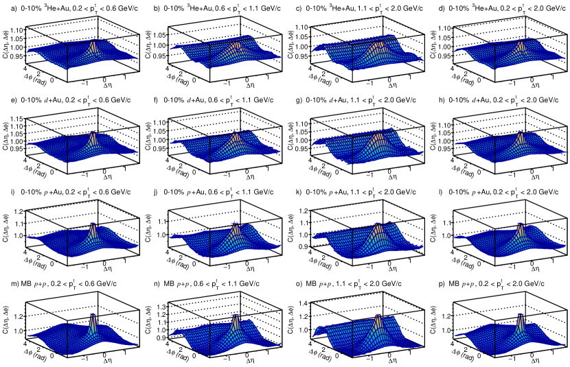
Figure 20: The normalized two-particle correlation function as a function of $\Delta\eta$ and $\Delta\phi$ for the trigger particles within different $p_{\mathrm{T}}$ ranges (from left to right) in the MB $p$$+$$p$ and the top 0–10% $p$$+$Au, $d$$+$Au and ³He$+$Au collisions at $\sqrt{s_{{}_{\mathrm{NN}}}}=200$ GeV(from bottom to top).

VIII Appendix: Additional plots

In this appendix, we present the original correlations that underlie the derivation of the $v_{n}$ results. Figure 20 displays the two-dimensional correlation functions across four $p_{\mathrm{T}}$ ranges from various collision systems. By analyzing these correlation functions, one can extract the one-dimensional correlation function within different $\Delta\eta$ intervals and subsequently convert it into per-trigger yields. These per-trigger yields are showcased in Figs. 21-24. For further context, Fig. 25 depicts a comparison of per-trigger yields in minimum-bias $p$$+$$p$ collisions between the collected data and the HIJING model.

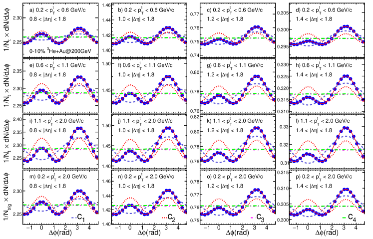
Figure 21: The per-trigger yield, $Y(\Delta\phi)$, as a function of $\Delta\phi$ for the trigger particles with different $p_{\mathrm{T}}$ (from top to bottom) and different $\Delta\eta$ (from left to right) selections in the 0–10% most central ³He$+$Au collisions at $\sqrt{s_{{}_{\mathrm{NN}}}}=200$ GeV. The color curves in each panel represent the Fourier components obtained from the Fourier expansion of the per-trigger yield.

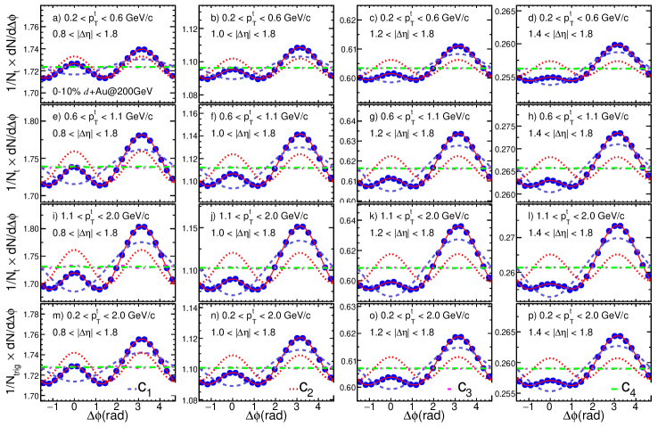
Figure 22: The per-trigger yield, $Y(\Delta\phi)$, as a function of $\Delta\phi$ for the trigger particles with different $p_{\mathrm{T}}$ (from top to bottom) and different $\Delta\eta$ (from left to right) selections in the 0–10% most central $d$$+$Au collisions at $\sqrt{s_{{}_{\mathrm{NN}}}}=200$ GeV. The color curves in each panel represent the Fourier components obtained from the Fourier expansion of the per-trigger yield.

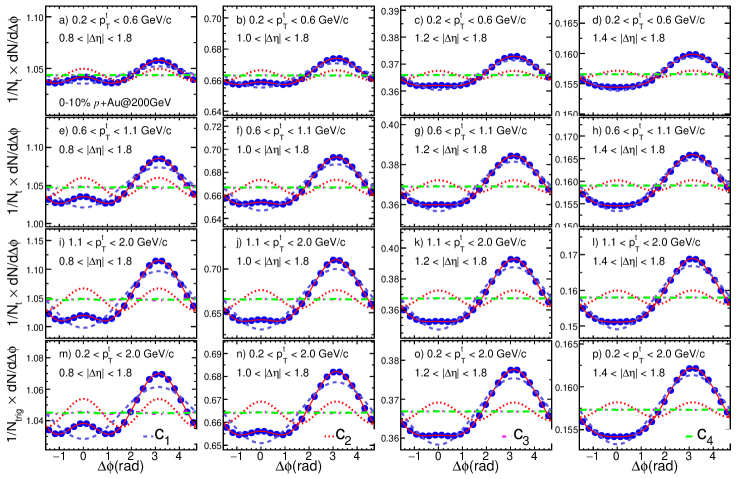
Figure 23: The per-trigger yield, $Y(\Delta\phi)$, as a function of $\Delta\phi$ for the trigger particles with different $p_{\mathrm{T}}$ (from top to bottom) and different $\Delta\eta$ (from left to right) selections in the 0–10% most central $p$$+$Au collisions at $\sqrt{s_{{}_{\mathrm{NN}}}}=200$ GeV. The color curves in each panel represent the Fourier components obtained from the Fourier expansion of the per-trigger yield.

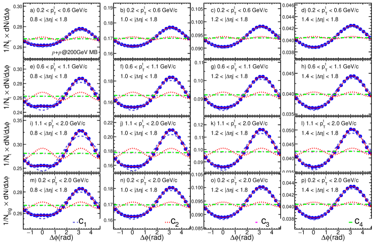
Figure 24: The per-trigger yield, $Y(\Delta\phi)$, as a function of $\Delta\phi$ for the trigger particles with different $p_{\mathrm{T}}$ (from top to bottom) and different $\Delta\eta$ (from left to right) selections in the MB $p$$+$$p$ collisions at $\sqrt{s_{{}_{\mathrm{NN}}}}=200$ GeV. The color curves in each panel represent the Fourier components obtained from the Fourier expansion of the per-trigger yield.

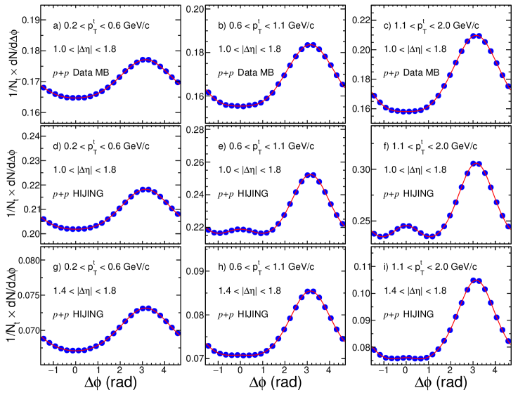
Figure 25: The per-trigger yield, $Y(\Delta\phi)$, as a function of $\Delta\phi$ for the trigger particles with different $p_{\mathrm{T}}$ (from left to right) and different $\Delta\eta$ (from top to bottom) selections in the $p$$+$$p$ collisions at $\sqrt{s_{{}_{\mathrm{NN}}}}=200$ GeV from both the STAR data (top row) and HIJING event generator (middle and bottom rows). The red lines through the data point indicate a fit including the first four Fourier harmonics.

References

- Busza et al. (2018) W. Busza, K. Rajagopal, and W. van der Schee, Ann. Rev. Nucl. Part. Sci. 68, 339 (2018), arXiv:1802.04801 [hep-ph] .
- Gale et al. (2013) C. Gale, S. Jeon, and B. Schenke, Int. J. Mod. Phys. A 28, 1340011 (2013), arXiv:1301.5893 [nucl-th] .
- Heinz and Snellings (2013) U. Heinz and R. Snellings, Ann. Rev. Nucl. Part. Sci. 63, 123 (2013), arXiv:1301.2826 [nucl-th] .
- Aad et al. (2012) G. Aad et al. (ATLAS), Phys.Rev. C86, 014907 (2012), arXiv:1203.3087 [hep-ex] .
- Khachatryan et al. (2010) V. Khachatryan et al. (CMS), JHEP 09, 091 (2010), arXiv:1009.4122 [hep-ex] .
- Aad et al. (2016) G. Aad et al. (ATLAS), Phys. Rev. Lett. 116, 172301 (2016), arXiv:1509.04776 [hep-ex] .
- Khachatryan et al. (2017) V. Khachatryan et al. (CMS), Phys. Lett. B 765, 193 (2017), arXiv:1606.06198 [nucl-ex] .
- Chatrchyan et al. (2013) S. Chatrchyan et al. (CMS), Phys. Lett. B 718, 795 (2013), arXiv:1210.5482 [nucl-ex] .
- Abelev et al. (2013) B. Abelev et al. (ALICE), Phys. Lett. B 719, 29 (2013), arXiv:1212.2001 [nucl-ex] .
- Aad et al. (2013) G. Aad et al. (ATLAS), Phys. Rev. Lett. 110, 182302 (2013), arXiv:1212.5198 [hep-ex] .
- Adare et al. (2013) A. Adare et al. (PHENIX), Phys. Rev. Lett. 111, 212301 (2013), arXiv:1303.1794 [nucl-ex] .
- Adare et al. (2015) A. Adare et al. (PHENIX), Phys. Rev. Lett. 114, 192301 (2015), arXiv:1404.7461 [nucl-ex] .
- Abdulameer et al. (2023) N. J. Abdulameer et al. (PHENIX), Phys. Rev. C 107, 024907 (2023), arXiv:2203.09894 [nucl-ex] .
- Abdulhamid et al. (2023) M. I. Abdulhamid et al. (STAR), Phys. Rev. Lett. 130, 242301 (2023), arXiv:2210.11352 [nucl-ex] .
- Aad et al. (2021a) G. Aad et al. (ATLAS), Phys. Rev. C 104, 014903 (2021a), arXiv:2101.10771 [nucl-ex] .
- Dusling et al. (2016) K. Dusling, W. Li, and B. Schenke, Int. J. Mod. Phys. E 25, 1630002 (2016), arXiv:1509.07939 [nucl-ex] .
- Schenke (2021) B. Schenke, Rept. Prog. Phys. 84, 082301 (2021), arXiv:2102.11189 [nucl-th] .
- Schenke et al. (2022) B. Schenke, S. Schlichting, and P. Singh, Phys. Rev. D 105, 094023 (2022), arXiv:2201.08864 [nucl-th] .
- Schenke et al. (2015) B. Schenke, S. Schlichting, and R. Venugopalan, Phys. Lett. B 747, 76 (2015), arXiv:1502.01331 [hep-ph] .
- Mace et al. (2018) M. Mace, V. V. Skokov, P. Tribedy, and R. Venugopalan, Phys. Rev. Lett. 121, 052301 (2018), [Erratum: Phys.Rev.Lett. 123, 039901 (2019)], arXiv:1805.09342 [hep-ph] .
- Mace et al. (2019) M. Mace, V. V. Skokov, P. Tribedy, and R. Venugopalan, (2019), arXiv:1901.10506 [hep-ph] .
- He et al. (2016) L. He, T. Edmonds, Z.-W. Lin, F. Liu, D. Molnar, and F. Wang, Phys. Lett. B 753, 506 (2016), arXiv:1502.05572 [nucl-th] .
- Kurkela et al. (2019) A. Kurkela, U. A. Wiedemann, and B. Wu, Eur. Phys. J. C 79, 759 (2019), arXiv:1805.04081 [hep-ph] .
- Romatschke (2018) P. Romatschke, Eur. Phys. J. C 78, 636 (2018), arXiv:1802.06804 [nucl-th] .
- Kurkela et al. (2021) A. Kurkela, A. Mazeliauskas, and R. Törnkvist, JHEP 11, 216 (2021), arXiv:2104.08179 [hep-ph] .
- Weller and Romatschke (2017) R. D. Weller and P. Romatschke, Phys. Lett. B 774, 351 (2017), arXiv:1701.07145 [nucl-th] .
- Gardim et al. (2012) F. G. Gardim, F. Grassi, M. Luzum, and J.-Y. Ollitrault, Phys. Rev. C 85, 024908 (2012), arXiv:1111.6538 [nucl-th] .
- Niemi et al. (2013) H. Niemi, G. S. Denicol, H. Holopainen, and P. Huovinen, Phys. Rev. C 87, 054901 (2013), arXiv:1212.1008 [nucl-th] .
- Alver et al. (2008) B. Alver, M. Baker, C. Loizides, and P. Steinberg, (2008), arXiv:0805.4411 [nucl-ex] .
- Nagle et al. (2014) J. L. Nagle, A. Adare, S. Beckman, T. Koblesky, J. Orjuela Koop, D. McGlinchey, P. Romatschke, J. Carlson, J. E. Lynn, and M. McCumber, Phys. Rev. Lett. 113, 112301 (2014), arXiv:1312.4565 [nucl-th] .
- Aidala et al. (2019) C. Aidala et al. (PHENIX), Nature Phys. 15, 214 (2019), arXiv:1805.02973 [nucl-ex] .
- Welsh et al. (2016) K. Welsh, J. Singer, and U. W. Heinz, Phys. Rev. C 94, 024919 (2016), arXiv:1605.09418 [nucl-th] .
- Mäntysaari and Schenke (2016) H. Mäntysaari and B. Schenke, Phys. Rev. Lett. 117, 052301 (2016), arXiv:1603.04349 [hep-ph] .
- Khachatryan et al. (2015) V. Khachatryan et al. (CMS), Phys. Rev. C 92, 034911 (2015), arXiv:1503.01692 [nucl-ex] .
- Aaboud et al. (2018) M. Aaboud et al. (ATLAS), Eur. Phys. J. C 78, 142 (2018), arXiv:1709.02301 [nucl-ex] .
- Aad et al. (2021b) G. Aad et al. (ATLAS), Phys. Rev. Lett. 126, 122301 (2021b), arXiv:2001.04201 [nucl-ex] .
- Bozek et al. (2011) P. Bozek, W. Broniowski, and J. Moreira, Phys. Rev. C 83, 034911 (2011), arXiv:1011.3354 [nucl-th] .
- Jia and Huo (2014) J. Jia and P. Huo, Phys. Rev. C 90, 034915 (2014), arXiv:1403.6077 [nucl-th] .
- Bozek and Broniowski (2016) P. Bozek and W. Broniowski, Phys. Lett. B 752, 206 (2016), arXiv:1506.02817 [nucl-th] .
- Pang et al. (2016) L.-G. Pang, H. Petersen, G.-Y. Qin, V. Roy, and X.-N. Wang, Eur. Phys. J. A 52, 97 (2016), arXiv:1511.04131 [nucl-th] .
- Shen and Schenke (2018) C. Shen and B. Schenke, Phys. Rev. C 97, 024907 (2018), arXiv:1710.00881 [nucl-th] .
- Bozek and Broniowski (2018) P. Bozek and W. Broniowski, Phys. Rev. C 97, 034913 (2018), arXiv:1711.03325 [nucl-th] .
- Zhao et al. (2022) W. Zhao, C. Shen, and B. Schenke, Phys. Rev. Lett. 129, 252302 (2022), arXiv:2203.06094 [nucl-th] .
- Zhao et al. (2023) W. Zhao, S. Ryu, C. Shen, and B. Schenke, Phys. Rev. C 107, 014904 (2023), arXiv:2211.16376 [nucl-th] .
- Acharya et al. (2022) U. A. Acharya et al. (PHENIX), Phys. Rev. C 105, 024901 (2022), arXiv:2107.06634 [hep-ex] .
- Note (1) This calculation uses instead of , and exhibit larger hierarchical differences, as shown in Table 1.
- Llope et al. (2014) W. J. Llope et al., Nucl. Instrum. Meth. A 759, 23 (2014), arXiv:1403.6855 [physics.ins-det] .
- Bieser et al. (2003) F. S. Bieser et al., Nucl. Instrum. Meth. A 499, 766 (2003).
- Adler et al. (2001) C. Adler, A. Denisov, E. Garcia, M. J. Murray, H. Strobele, and S. N. White, Nucl. Instrum. Meth. A 470, 488 (2001), arXiv:nucl-ex/0008005 .
- Adamczyk et al. (2012) L. Adamczyk et al. (STAR), Phys. Rev. D 86, 072013 (2012), arXiv:1204.4244 [nucl-ex] .
- Llope (2012) W. J. Llope (STAR), Nucl. Instrum. Meth. A 661, S110 (2012).
- Szelezniak (2015) M. Szelezniak, PoS Vertex2014, 015 (2015).
- Abelev et al. (2010) B. I. Abelev et al. (STAR), Phys. Rev. C 81, 024911 (2010), arXiv:0909.4131 [nucl-ex] .
- Anderson et al. (2003) M. Anderson et al., Nucl. Instrum. Meth. A 499, 659 (2003), arXiv:nucl-ex/0301015 .
- Kharzeev and Nardi (2001) D. Kharzeev and M. Nardi, Phys. Lett. B 507, 121 (2001), arXiv:nucl-th/0012025 .
- Abelev et al. (2009) B. I. Abelev et al. (STAR), Phys. Rev. C 79, 034909 (2009), arXiv:0808.2041 [nucl-ex] .
- Adare et al. (2008) A. Adare et al. (PHENIX), Phys. Rev. C 78, 014901 (2008), arXiv:0801.4545 [nucl-ex] .
- Adams et al. (2004) J. Adams et al. (STAR), Phys. Rev. Lett. 93, 252301 (2004), arXiv:nucl-ex/0407007 .
- Adams et al. (2005) J. Adams et al. (STAR), Phys. Rev. C 72, 014904 (2005), arXiv:nucl-ex/0409033 .
- Aad et al. (2014) G. Aad et al. (ATLAS), Phys. Rev. C 90, 044906 (2014), arXiv:1409.1792 [hep-ex] .
- Adare et al. (2018) A. Adare et al. (PHENIX), Phys. Rev. C 98, 014912 (2018), arXiv:1711.09003 [hep-ex] .
- Lim et al. (2019) S. H. Lim, Q. Hu, R. Belmont, K. K. Hill, J. L. Nagle, and D. V. Perepelitsa, Phys. Rev. C 100, 024908 (2019), arXiv:1902.11290 [nucl-th] .
- Liu et al. (2020) Z. Liu, A. Behera, H. Song, and J. Jia, Phys. Rev. C 102, 024911 (2020), arXiv:2002.06061 [nucl-ex] .
- Romatschke (2015) P. Romatschke, Eur. Phys. J. C 75, 305 (2015), arXiv:1502.04745 [nucl-th] .
- Schenke et al. (2020a) B. Schenke, C. Shen, and P. Tribedy, Phys. Lett. B 803, 135322 (2020a), arXiv:1908.06212 [nucl-th] .
- Schenke et al. (2020b) B. Schenke, C. Shen, and P. Tribedy, Phys. Rev. C 102, 044905 (2020b), arXiv:2005.14682 [nucl-th] .
- Wang et al. (2017) X. Wang, F. Shen, S. Wang, C. Feng, C. Li, P. Lu, J. Thomas, Q. Xu, and C. Zhu, Nucl. Instrum. Meth. A 859, 90 (2017), arXiv:1704.04339 [physics.ins-det] .
- Adams et al. (2020) J. Adams et al., Nucl. Instrum. Meth. A 968, 163970 (2020), arXiv:1912.05243 [physics.ins-det] .
- Başar and Teaney (2014) G. Başar and D. Teaney, Phys. Rev. C 90, 054903 (2014), arXiv:1312.6770 [nucl-th] .
- Giacalone et al. (2021) G. Giacalone, J. Jia, and C. Zhang, Phys. Rev. Lett. 127, 242301 (2021), arXiv:2105.01638 [nucl-th] .
- Aaboud et al. (2019) M. Aaboud et al. (ATLAS), Phys. Lett. B 789, 444 (2019), arXiv:1807.02012 [nucl-ex] .