Empirical Validation of Conformal Prediction for Trustworthy Skin Lesions Classification

Abstract

Uncertainty quantification is a pivotal field that contributes to the realization of reliable and robust systems. By providing complementary information, it becomes instrumental in fortifying safe decisions, particularly within high-risk applications. Nevertheless, a comprehensive understanding of the advantages and limitations inherent in various methods within the medical imaging field necessitates further research coupled with in-depth analysis. In this paper, we explore Conformal Prediction, an emerging distribution-free uncertainty quantification technique, along with Monte Carlo Dropout and Evidential Deep Learning methods. Our comprehensive experiments provide a comparative performance analysis for skin lesion classification tasks across the three quantification methods. Furthermore, We present insights into the effectiveness of each method in handling Out-of-Distribution samples from domain-shifted datasets. Based on our experimental findings, our conclusion highlights the robustness and consistent performance of conformal prediction across diverse conditions. This positions it as the preferred choice for decision-making in safety-critical applications.

1 Introduction

Deep learning algorithms have demonstrated significant potential in solving a wide range of complex, real-world problems [1]. These algorithms’ capacity to autonomously learn intricate patterns and representations makes them valuable in diverse computer vision tasks, including image classification [2, 3], object detection [4], and remote sensing [5]. Generally, the evaluation of deep learning algorithms relies on accuracy as the main metric to assess how well the model has learned from the training data. While accuracy is widely acknowledged in the literature, it alone does not guarantee the system’s robustness. This is more apparent in safety-critical applications where errors in decision-making can have catastrophic consequences [6]. To mitigate the risk of erroneous decisions, presenting the confidence level associated with predictions made by deep learning algorithms is imperative. For this purpose, uncertainty quantification techniques are instrumental in providing models with additional information that presents prediction confidence and ultimately helps improve the model’s robustness.

In machine learning, two sources of uncertainties collectively influence model predictions [7]. The first source, known as epistemic uncertainty, arises from a lack of knowledge and understanding. Model retraining and incorporating additional information and data are typically employed to mitigate this type of uncertainty [8]. The second source of uncertainty is aleatoric uncertainty, which characterizes the inherent randomness within the data and, as such, remains irreducible. In the existing literature, various approaches offer both theoretical and practical solutions for quantifying uncertainties associated with deep learning models. These methods can be broadly categorized into Single Deterministic Networks, Bayesian Neural Networks, Deep Ensembles, and Test-time Augmentation methods [9].

Single deterministic networks are straightforward methods to represent the predictive uncertainty of deep learning models. As suggested by the name, the networks are trained to adjust their weights in a deterministic manner, and the uncertainty is measured through a single forward pass. A simple baseline of single deterministic networks is the utilization of the neural network output probabilities (i.e., SoftMax outputs for classification) as an interpretation of the model uncertainty. Several studies, however, showed that neural networks are often over-confident [10], hence their output probabilities are miscalibrated [11] and tend to generate wrong uncertainty estimates. A more generic approach in single deterministic networks includes predicting the parameters of a prior distribution over the outputs. such algorithms are known as Evidential learning [12] or Prior Networks [13]. The framework of these approaches involves introducing a higher-order distribution over the likelihood function, with the parameters of these distributions being estimated using the underlying neural network. The predicted class probability corresponds to the expected value of the distribution, while the variance of the distribution serves as an estimate of the model’s uncertainty.

Bayesian Neural Networks (BNNs) [14] seamlessly merge the principles of Bayesian inference with traditional neural networks. Instead of considering BNN parameters as fixed, deterministic values, they are treated as probability distributions. This unique approach empowers BNNs to effectively capture and represent predictive uncertainty. Consider a neural network with parameters $\omega$ and a training dataset $D_{t}=(x,y)$. If the network weights are assigned a prior distribution, denoted as $P(\omega)$, the posterior distribution $P(\omega|x,y)$ can be calculated using Bayes’ theorem. To calculate the posterior $p(\omega|X,Y)$, it necessitates integrating over all possible values of $\omega$, a task that is often intractable. Generally, obtaining the posterior is only viable through either Variational Inference [15], where a simple and tractable distribution is used to approximate the exact posterior, or through other approximation techniques, such as Markov Chain Monte Carlo (MCMC) [16].

Deep ensembles involve training several deep networks with random initializations on a given dataset and deriving a unified prediction from the collective outputs of the ensemble members [17]. Although initially designed to improve prediction accuracy, deep ensembles have shown their capacity to effectively estimate predictive uncertainties in various studies. Consider a $M$ number of independent networks that map the inputs $x$ to a label $y$, such that $y=f_{\theta_{i}}(x)$, each network is parameterized by $\theta$ parameters, and $i\in 1,\ldots,M$. The combined prediction of the ensemble can be simply represented as the average predictions of each network at inference.

Recently, Conformal prediction (CP) [18, 19] emerged as a prominent uncertainty quantification technique. It has gained attention in the fields of machine learning and computer vision [20, 21]. In addition to its elegance and computational efficiency, CP algorithms belong to the domain of ’distribution-free’ methodologies. This implies that they are model-agnostic, data distribution agnostic, and applicable to finite sample sizes.

In this paper, we compare three top-performing uncertainty quantification methods, namely CP, Monte Carlo Dropout (MCD), and Evidential Deep Learning (EDL), and provide a comprehensive and detailed analysis of their performance. We include three experiments to underscore the unique attributes of each method, with a particular emphasis on CP, a less-explored approach for skin lesion classification tasks. The main contributions of our work are as follows:

1. We proposed in-depth explorations and analysis of three deep-learning uncertainty quantification techniques, including the prominent emerging CP, for the classification task of skin lesions.

2. We presented a comparative analysis and comprehensive evaluation of the implication of CP parameter variations. Particularly, we studied the effect of changing the scoring function, the confidence level, and the calibration set size through a detailed set of requirements.

3. We conducted an assessment of the effectiveness of each method in addressing Out-of-Distribution (OOD) data arising from covariate shifts.

The remainder of this paper is organized as follows: Section 2 presents background on uncertainty quantification techniques and the related work to our study. Section 3 presents the experiment settings, the experiment results, and the discussions. Section 4 concludes the paper and proposes future work directions.

2 Background on Uncertainty quantification Methods

In the rich domain of uncertainty quantification, understanding the nuances of existing methodologies and their implementation details is paramount. This section delves into the background literature and related work that forms the foundation for uncertainty methods, We specifically focus on three quantification techniques that form the basis of our experimental analysis. For a more comprehensive review of uncertainty quantification methods in deep learning, interested readers can refer to [9, 22, 23].

2.1 Monte Carlo Dropout

Dropout is a common practice during training to prevent overfitting, involving the random deactivation of neurons in the network. In their research, Gal et al [24]. demonstrated that dropout can also serve as a Bayesian approximation, enabling the prediction of the network’s uncertainty when applied during inference. A straightforward method to estimate the network’s uncertainty involves enabling dropout during inference and conducting multiple forward passes of the same input. The random deactivation of neurons during this process introduces variability in the outputs, resulting in both a mean and a variance. The mean value serves as the prediction, while the variance serves as an estimate of the prediction’s uncertainty.

In the case of N multiple passes, Let $f(x)$ be the prediction of the neural network for input $x$. During MCD, we obtain $T$ samples of predictions $f_{t}(x)$ where $t=1,2,...,T$ represents each Monte Carlo sample. The mean prediction can be represented as:

$$\hat{f}(x) =\frac{1}{T}\sum_{t=1}^{T}f_{t}(x)$$ (1)

The uncertainty can be expressed as the variance of these predictions:

$$\text{{Var}}(x)=\frac{1}{T}\sum_{t=1}^{T}\left(f_{t}(x)-\frac{1}{T}\sum_{t^{\prime}=1}^{T}f_{t^{\prime}}(x)\right)^{2}$$ (2)

2.2 Evidential Deep Learning

In a traditional Convolution Neural Network (CNN), label probabilities are generated by applying a SoftMax activation function to the last layer. The objective is to maximize the likelihood function by minimizing a metric of loss, often a cross-entropy loss, which tends to make the prediction "overconfident" [25]. The output of the SoftMax operation reflects discrete point estimates of class probabilities without proper indication of the uncertainty present in the estimate. EDL on the other hand accounts for the uncertainties in prediction by estimating output distributions instead of rigid labels [12]. The Dempster-Shafer theory of evidence (DST) [26] and Subjective Logic (SL) provide a well-defined approach to quantifying class uncertainties. The approach suggests that for a $K$ class network, with a belief mass $b_{k}$ assigned to each class label $k\in K$, an overall uncertainty is $u$ can be expressed, such that:

$$u+\sum_{k=1}^{K}b_{k}=1$$ (3)

The output of the neural network model (before the conventional SoftMax layer, referred to as logits) is trained to represent the evidence vectors $e_{k}$. These evidence vectors represent the amount of support on how confident a sample is, given a particular class. The vectors relate to the belief masses and uncertainties as follows:

$$b_{k}=\frac{e_{k}}{S},\quad u=\frac{K}{S},\quad\textit{where,}\quad S=\sum_{k=1}^{K}(e_{k}+1)$$ (4)

It is interesting to note that the uncertainty value from Equation 4 is inversely proportional to $S$, which represents the sum of evidence and the number of labels. This notes that a zero-evidence vector would yield a belief mass $b_{k}=0$, and the maximum uncertainty $u=1$. The likelihood function for classification models learns over a categorical distribution. EDL places a higher order distribution over the parameters of the categorical distribution (label probabilities) to allow for prediction uncertainty estimation $u$. To ensure a tractable posterior, it is essential to select a prior conjugate distribution, such as the Dirichlet distribution. Parameterized by $\alpha=[\alpha_{1},...,\alpha_{K}]$, the Dirichlet distribution’s density function is expressed by:

$$D(\mathbf{p}\mid\alpha)=\frac{1}{\beta(\alpha)}\prod_{k=1}^{K}p_{k}^{\alpha_{k}-1}$$ (5)

Where $\mathbf{p}$ is the probability mass function, $\beta(\alpha)$ is the Beta function, $p_{k}$ is the probability for label $k$ and $\alpha_{k}$ can be calculated as $\alpha_{k}=e_{k}+1$. The probability of each class is equivalent to the expectation of the Dirichlet distribution:

$$\mathbb{E}[D(\alpha)]=\frac{\alpha_{k}}{S}$$ (6)

The $S$ here is taken from Equation LABEL:uncertainty and can be referred to as the strength of the Dirichlet distribution.

A Kullback-Leibler (KL) divergence is used to regularize the prediction of the network. The term measures the similarities of the predicted distribution to a uniform Dirichlet distribution with $\alpha_{k}=1$ $\forall$ $k\in K$ or zero evidence. The KL term is added to the loss function, and therefore, penalizes samples that deviate from class categories. The KL term is given by:

$$KL[D(p_{i}\mid\tilde{\alpha}_{i})\mid\mid D(p_{i}\mid 1)]=\\ \log\bigg{(}\frac{\Gamma(\sum_{k=1}^{K}\tilde{\alpha}_{ik})}{\Gamma(K)\prod_{k=a}^{K}\Gamma(\tilde{\alpha}_{ik})}\bigg{)}+\sum_{k=1}^{K}(\tilde{\alpha}_{ik}-1)\Big{[}\psi(\tilde{\alpha}_{ik})-\psi\Big{(}\sum_{j=1}^{K}\tilde{\alpha}_{ik}\Big{)}\Big{]}$$ (7)

Where $\tilde{\alpha}_{ik}=y_{i}+(1-y_{i})\odot\alpha_{i}$ is the modified Dirichlet parameter. $\Gamma$ is the Gamma function and $\psi$ is the Digamma function.

2.3 Conformal Prediction

CP, an emerging method for quantifying uncertainty, has garnered attention in the fields of machine learning and computer vision. Renowned for its simple implementation, computational efficiency, and versatility across various models, CP techniques have become increasingly prominent. They can be applied to a wide range of pre-trained models, including decision support models, shallow multi-layer perceptrons, deep neural networks, and more. Additionally, they can be deployed for various tasks such as classification or regression. Furthermore, these methods do not require any assumptions about the underlying data distribution. Additionally, they provide a guarantee of validity, even when working with a finite number of samples. Hence, CP proves to be indispensable across a broad spectrum of real-world applications.

Unlike other uncertainty quantification methods, the output of the CP algorithm is a prediction set of all possible labels such that the true label is included within this set with a user-defined confidence level. The implementation of CP only requires a model $f$ trained conventionally on a given dataset, and an additional small independent and identically distributed (i.i.d) dataset, which we will refer to as the calibration dataset. To understand the underlying details of CP, consider a classification task where a deep learning model is trained on a dataset of images $x_{\text{train}}$ to correctly classify each input image to its corresponding $y_{\text{train}}$ label chosen from $K$ total classes. The class probability outputs, i.e., SoftMax function $\sigma$, are utilized as a notion of model uncertainty and used to derive the conformity scores as $S=\sigma(f(x))$. Furthermore, a designated $C$ subset of sample images and their true labels are reserved for the calibration, where $C=\{(X_{n},Y_{n}),n=1,\ldots,N\}$. Both $S$ and $C$ are used to construct a function $\mathcal{T}$ that returns a prediction set of possible labels. The process of finding $T$ includes passing all samples $X_{n}$ $\in$ $C$ to the model, collecting their $N$ conformity score of the correct label $S(X_{n},Y_{n})=\sigma(f(X_{n})_{y}$, and finally calculating $\hat{q}$ which is the empirical quantile of the scores using the user-defined error rate $\alpha\in[0,1]$ and the size of the calibration set $N$:

$$\hat{q}=\frac{\left\lceil(1+N)(1-\alpha)\right\rceil}{N}$$ (8)

For a new fresh pair $(x_{\text{test}},y_{\text{test}})$, the conformity score is calculated, and the prediction set is generated to include the labels whose score values are less than $\hat{q}$:

$$\mathcal{T}(x_{\text{test}})=\{y:S(x_{\text{test}})\leq\hat{q}\}$$ (9)

The resulting prediction set guarantees the conformal coverage criteria, with the following probability:

$$1-\alpha\leq P(Y_{\text{test}}\in T(x_{\text{test}}))\leq(1-\alpha)+\frac{1}{1+M}$$ (10)

The design of the scoring function is a critical element that requires careful engineering. This scoring function encapsulates all the information embedded in the model; thus, a robust scoring function is essential for generating a meaningful conformal set. It’s important to emphasize that the preceding steps can be extended to include a variety of tasks, including regression. The sole variation in the steps outlined above lies in the choice of a scoring function tailored to the specific requirements of the given task.

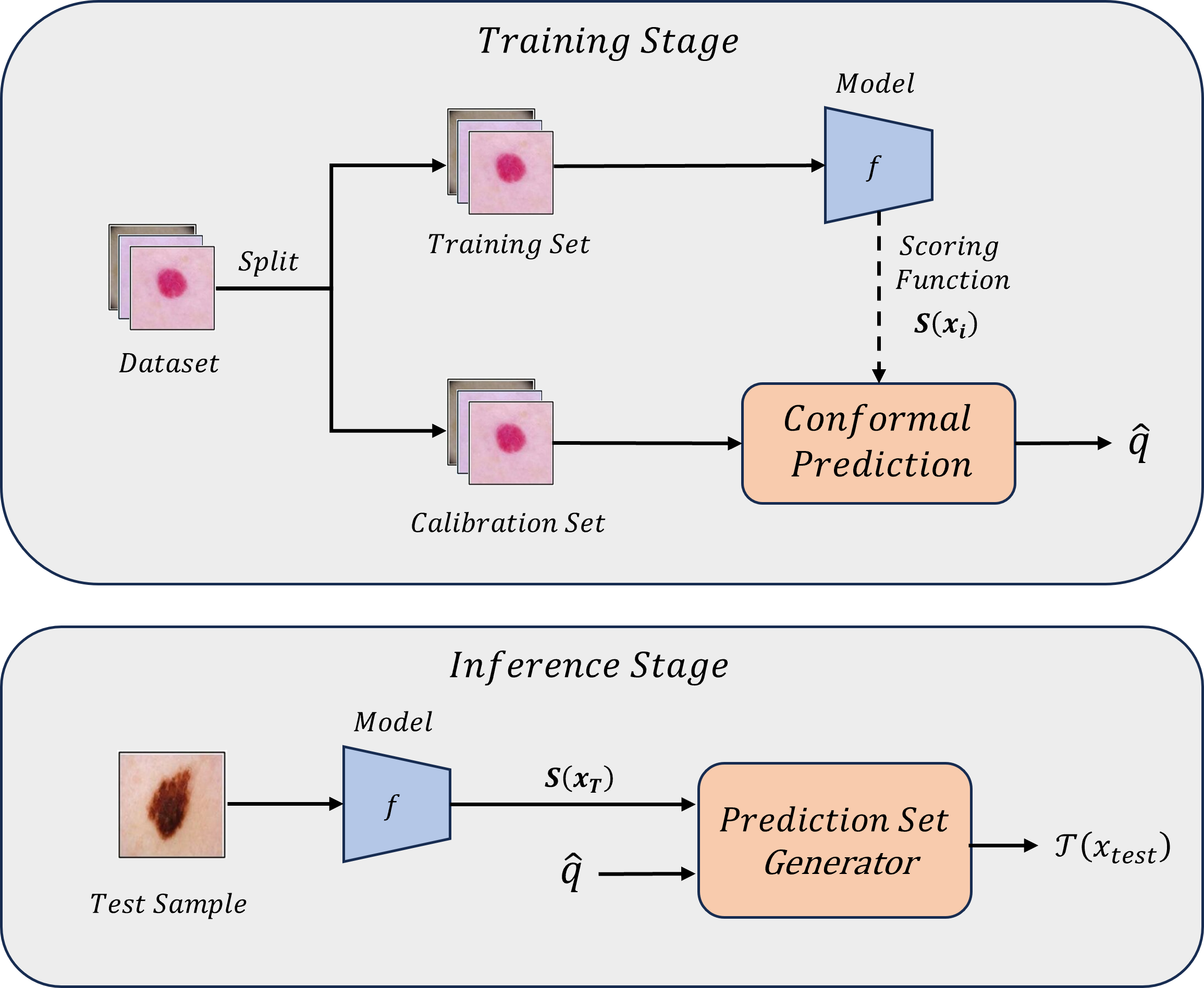
Figure 1: Conformal Prediction Framework. The dataset is split into a training set, a calibration set, and a testing set. Conformal Prediction utilizes the scoring function and calibration set to generate a quantile value. At inference, a test sample is passed to the train network, and the output score along with the quantile value is used to generate prediction sets.

3 Expirements and Results

3.1 Dataset

This paper focuses on the challenge of classifying different types of skin lesions by leveraging deep learning approaches and medical images. For this purpose, we work on the HAM10000 dataset [27], which contains more than 10,000 images captured from real patients with seven distinct lesion classes. The HAM10000 dataset is highly imbalanced, with some classes having more samples than others. To mitigate bias, we applied data augmentation techniques such as flipping and rotations to increase the number of samples in less-represented classes. To train the network, we divided the dataset into 50% training, 20% validation, and 30% for testing. We used samples from both validation and testing datasets to form the calibration dataset used in CP.

3.2 Expiremental Setup

3.2.1 Model Specifications and Training configuration

In all our experiments, ResNet-18 [28] was adopted as the underlying core network for all the uncertainty quantification methods. The network consists of 18 layers, which include convolutional layers, batch normalization, dropout layers, ReLU activation functions, and residual blocks. A classification head is modified to classify the input images into their corresponding 7 classes. We trained the core model using the cross-entropy loss for 100 epochs. The Adam optimizer was used with a learning rate of 1e-4. A learning rate scheduler was added to reduce the learning rate by 0.5 when the validation loss is not improved for 10 consecutive epochs. All the experiments are run on an NVIDIA RTX A5000.

3.2.2 Uncertainty Quantification Models

As previously indicated, the ResNet-18 model serves as the foundational architecture for implementing uncertainty quantification methods. However, distinct modifications are necessitated to incorporate each of the three uncertainty quantification techniques. In this section, we elaborate on the required design settings tailored for the implementation of each method. Furthermore, we address any supplementary training configurations and methodologies employed in the integration of the core model to the uncertainty quantification technique.

CP, as a post-hoc technique, obviates the need for retraining the core network. The implementation simply involves reserving a portion of the dataset, unused during the training phase, for calibration. Following the work in [29] , we assigned 1000 calibration data samples. Furthermore, we have assigned the confidence level to 90%. The overall algorithm is summarized in Algorithm 1. Moreover, the effect of changing the calibration size and the confidence level are further studied in Section 3.4.

Algorithm 1 APS

1:input: (model, calibration set, new input)

2:get scores: Apply the scoring function to all training images as: $E_{j}=\sum_{i=1}^{k^{\prime}}(\hat{\pi}_{(i)}(x_{j})$ where $k^{\prime}$ is the model’s ranking of the true class $y_{j}$, and $\hat{\pi}_{(i)}(x_{j})$ is $i^{th}$ largest score for the $j^{th}$ input.

3:Compute $\hat{q}$: The value corresponding to the $1-\alpha$ quantile of $E_{j}$

4:Output prediction set: $\sum_{i=1}^{k^{*}}(\hat{\pi}_{(i)}(x+1))\geq\hat{q}$

For the implementation of MCD, a dropout layer with a rate of 0.5 was added to the primary ResNet-18 model, positioned before the last classification layer. The uncertainty estimation process entailed conducting 1000 forward passes during the inference stage.

Unlike CP and MCDropout, the EDL algorithm requires retraining the model with different settings. The conventional cross-entropy loss function is replaced with a mean square error loss function, tailored to estimate the $\alpha$ parameters of the Dirichlet distribution, which is used to estimate the predictive uncertainty. The loss function is presented by:

$$\mathcal{L}_{i}(\theta)=\sum_{j=1}^{K}(y_{ij}-\frac{\alpha_{ij}}{S_{i}})^{2}+\frac{\alpha_{ij}(S_{i}-\alpha_{ij})}{S_{i}^{2}(S_{i}+1)}$$ (11)

where $y_{ij}$ is the ground truth class label, $\alpha_{ij}$ is the corresponding Dirichlet parameter, and $S$ is the strength of the Dirichlet distribution, as expressed in Equation 4. Similar to the previous optimizer settings, the Adam optimizer is used with a learning rate of 1e-5, and the model was trained for 150 epochs.

3.3 Evaluation of Uncertainty Quantification methods

This section presents a quantitative assessment and comparative analysis of the three uncertainty quantification methods: CP, MCD, and EDL. Initially, the base classification model was trained without the incorporation of any uncertainty method. The model achieves an 86.7% accuracy rate on the testing dataset that contains 1103 samples. In the context of CP, we set a user-defined confidence interval of $1-\alpha$, where $\alpha$ is chosen to be 0.10, corresponding to a 90% confidence level. This implies that the ground truth label is encompassed within the generated prediction sets with a 90% confidence bound. A larger prediction set indicates higher predictive uncertainty, while a smaller set implies lower uncertainty. As mentioned earlier, CP operates as an add-on algorithm, acting on the SoftMax probabilities produced by the core model. Consequently, deploying CP does not alter the initial accuracy of the model. In the context of predictive uncertainty, CP assigns a mean uncertainty value of 0.40 to correctly classified samples and 0.79 to wrongly classified samples. Meanwhile, for the MCD method, 1000 forward passes are executed during inference to estimate the model’s uncertainty, resulting in an accuracy of 85.8%. Noteworthy is that correctly classified examples in MCD are associated with a mean uncertainty value of 0.01, whereas wrongly classified examples exhibit a mean uncertainty value of 0.09. In contrast, EDL takes a distinct approach by being trained from scratch using the mean square error loss that explicitly accounts for uncertainties. The EDL model achieves an accuracy of 85.7%, with a mean uncertainty value of 0.19 assigned to correctly classified samples and 0.51 to wrongly classified examples. The results are shown in Table 1.

UQ algorithm	Accuracy	$\mathbf{U_{\text{correct}}\pm\text{std}}$	$\mathbf{U_{\text{wrong}}\pm\text{std}}$	Retraining
MCD	85.8%	$0.01\pm 0.03$	$0.09\pm 0.04$	✗
EDL	85.7%	$0.19\pm 0.13$	$0.51\pm 0.25$	✓
CP	86.7%	$0.40\pm 0.3$	$0.79\pm 0.15$	✗

Table 1: Comparison of UQ Algorithms: Accuracy, Uncertainty Estimates, and Retraining Indicator. The table presents model accuracy along with mean uncertainty values for both correctly classified samples and wrongly classified samples, in addition to an indication of whether retraining was performed, for Monte Carlo Dropout (MCD), Evidential Deep Learning (EDL), and Conformal Prediction (CP).

Figure 2 showcases the histogram distributions of the assigned uncertainty values for correctly and wrongly classified samples, across the three aforementioned uncertainty quantification methods. The same is also illustrated in Figure 3 through the kernel density estimation plot, which offers a continuous representation of the probability density function for a more comprehensive understanding of the uncertainty characteristics across the dataset.

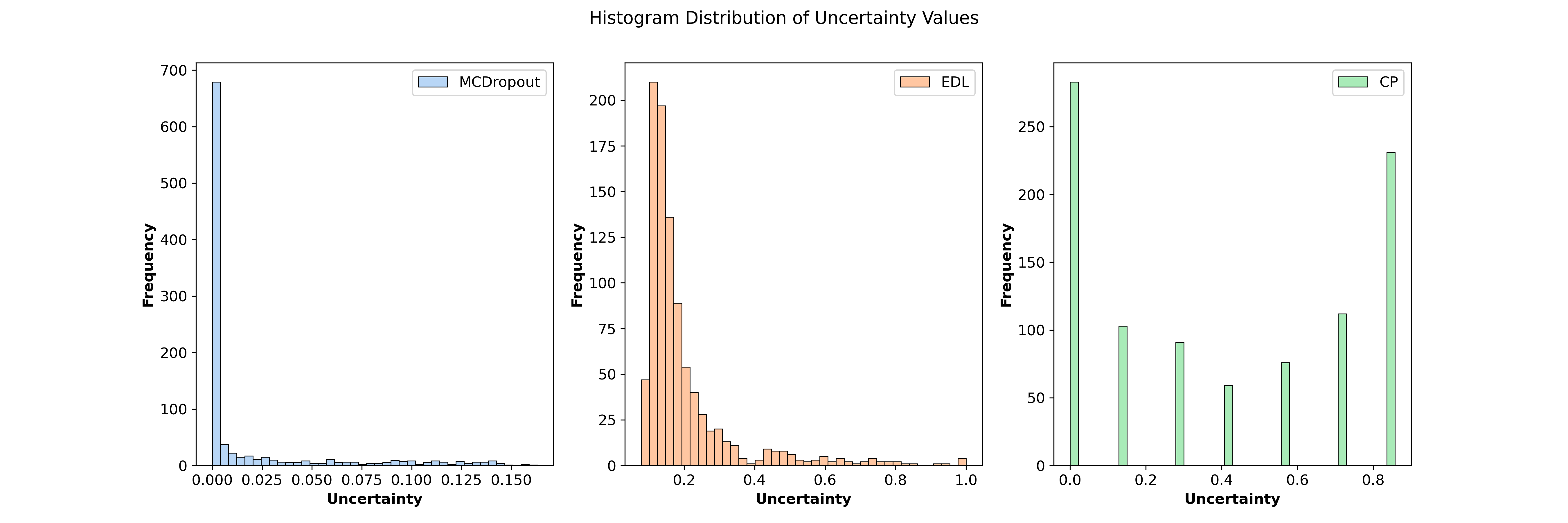
(a) Correctly classified samples

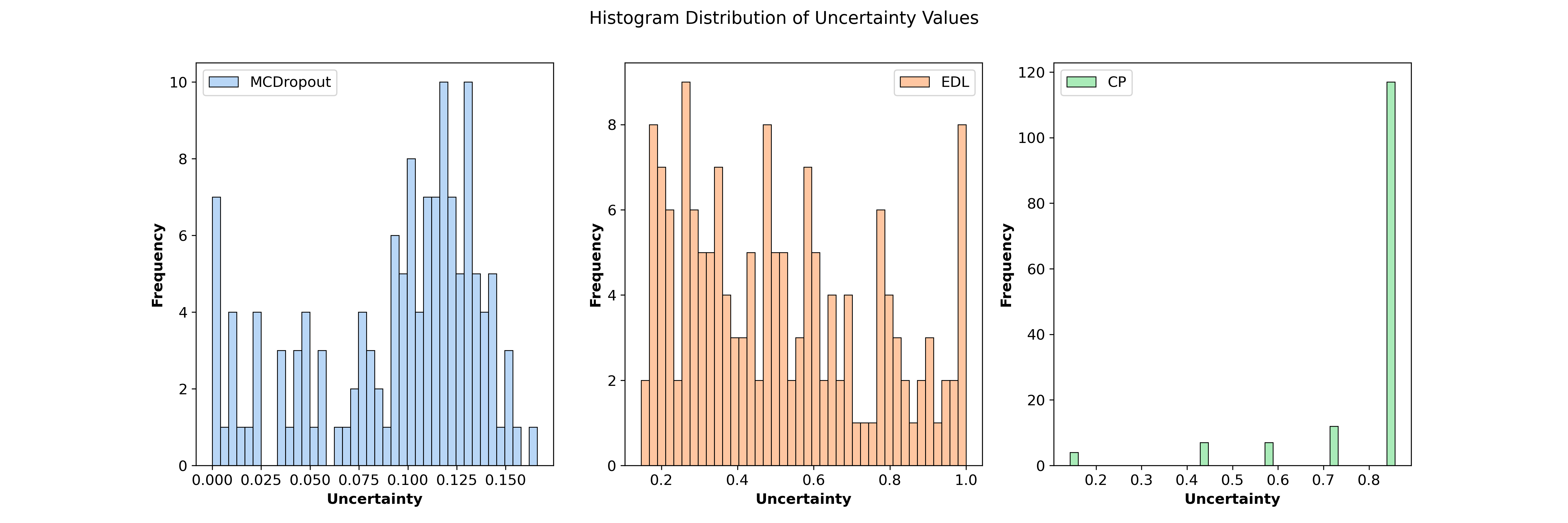
(b) Wrongly classified samples

Figure 2: The histogram distribution of uncertainty values assigned by each uncertainty quantification algorithm to both correctly and wrongly classified samples.

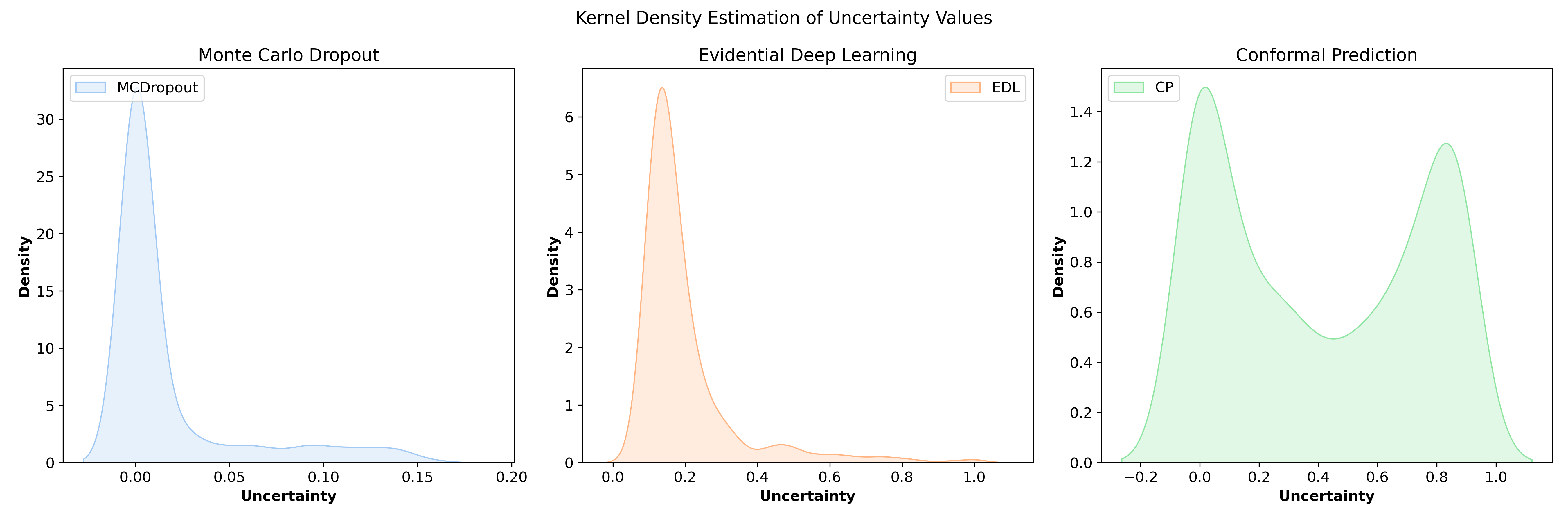
(a) Correctly classified samples

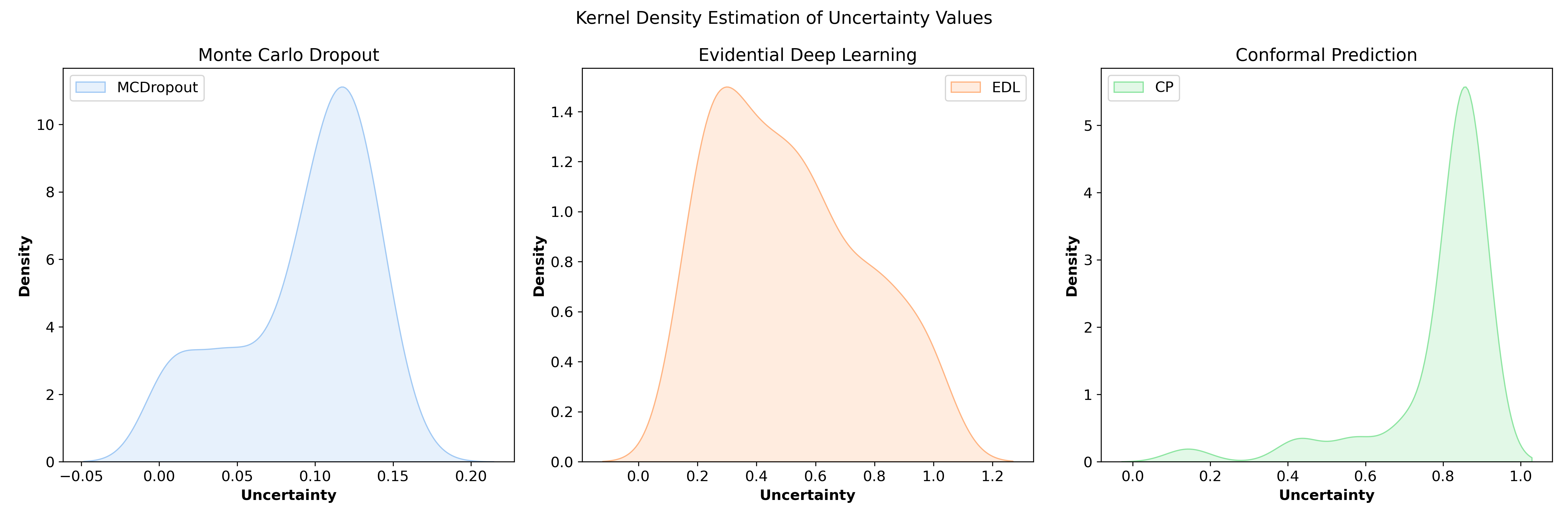
(b) Wrongly classified samples

Figure 3: The density distribution of uncertainty values assigned by each uncertainty quantification algorithm to both correctly and wrongly classified samples.

3.3.1 Discussion

In light of the conducted experiments, the obtained results provide valuable insights and analysis into uncertainty prediction techniques. Before discussing the advantages and drawbacks of each technique, it is imperative to emphasize that predictive uncertainty should not be misconstrued as a definitive indicator of classification output. Instead, it serves as supplementary information that enriches the model’s robustness. It’s typical to find correctly classified samples in the dataset with a mix of both high and low uncertainty values. The variability in uncertainty values is a result of the differences in difficulty levels among individual samples. Ideally, the uncertainty value of the wrongly classified samples should be consistently higher, indicating less confidence in the network’s output. As observed in Figure 2 and Figure 3, CP exhibits such behavior, where the majority of wrongly classified samples are assigned high uncertainty values. When examining the results for both MCD and EDL, we observe a flatter distribution for wrongly classified samples, suggesting a greater variability in uncertainty values.

Compared with MCD and EDL, CP stands out for its simplicity in implementation. The algorithm operates seamlessly, eliminating the need for retraining procedures or modifications to the model’s architecture. This crucial feature facilitates the quantification of uncertainties and ensures that the accuracy of the original model remains unaffected. In MCD, little modifications to the model architecture might be necessary to include dropout layers if not present. Nevertheless, MCD requires running multiple forward passes, contributing to an increased computational load. Moreover, it is crucial to note that high dropout rates have the potential to compromise accuracy, emphasizing the importance of carefully tuning dropout parameters to strike a balance between uncertainty quantification and model performance. Additionally, some studies show that MCD tends to output ill-calibrated uncertainty values that can be unreliable for uncertainty quantification [22]. EDL, on the other hand, generates sharp uncertainty distribution for the correctly classified samples, but a broad distribution with wrongly classified samples, making it less reliable. The implementation of EDL is relatively more complex when compared to CP and MCD. It requires modifying the core model, changing the training loss function, and retraining the modified model from scratch.

3.4 Sensitivity of Conformal Prediction Parameters

In this section, we delve into the details of the model’s performance by conducting a comprehensive sensitivity analysis on key CP parameters. We investigate the impact of three pivotal factors: first, the selection of the scoring function; second, the adjustment of the confidence level $\alpha$; and third, the variation in the calibration set size. Through this exploration, we aim to study the dependencies between these parameters and the model’s performance in the context of uncertainty estimation.

3.4.1 Scoring Function

The scoring function stands out as a critically significant element within the context of CP. While the CP algorithm consistently ensures marginal coverage by regulating the size of the prediction set, it is the scoring function that ultimately determines the utility of the set’s content the scoring function distinguishes whether the predictions included in the set are deemed useful or not. To this end, we study the effect of altering the scoring function and present analysis on two key terms: 1) The distribution of uncertainties on correctly classified samples Vs. wrongly classified samples and 2) the size of the prediction set.

To determine the effect of the scoring function, an additional variation of CP, known as Regularized Adaptive Prediction Sets (RAPS) [20] is implemented. RAPS takes the SoftMax outputs, similar to the APS method implemented in our experimental results, however, it adds a regularization term to the extremely large prediction sets to discourage their presence in the final prediction set. As a result, the average prediction set size produced by RAPS is much smaller than that produced by APS. The RAPS algorithm is summarized in Algorithm 2

Algorithm 2 RAPS

1:input: (model, calibration set, new input)

2:get scores: Apply the scoring function to all training images as: $E_{j}=\sum_{i=1}^{k^{\prime}}(\hat{\pi}_{(i)}(x_{j})+\lambda\textbf{1}[i>k_{\text{reg}}]),$ where $k^{\prime}$ is the model’s ranking of the true class $y_{j}$, and $\hat{\pi}_{(i)}(x_{j})$ is $i^{th}$ largest score for the $j^{th}$ input.

3:Compute $\hat{q}$: The value corresponding to the $1-\alpha$ quantile of $E_{j}$

4:Output prediction set: $\sum_{i=1}^{k^{*}}(\hat{\pi}_{(i)}(x+1)+\lambda\textbf{1}[j>k_{\text{reg}}])\geq\hat{q}$

Results presented in Table 2 show that RASP produces an average prediction set size smaller than that generated by APS. While smaller prediction set sizes are typically preferred as they imply greater certainty, this characteristic may pose challenges, particularly in instances of misclassified samples where the regularization term penalizes larger set sizes that show more uncertainty, as shown in Figure 4

Conformal Method	$C_{correct}$	$C_{wrong}$	Average
ASP	2.84	5.54	4.19
RASP	1.19	2.35	1.77

Table 2: Comparison between the average prediction set size produced by APS and RAPS algorithms for correctly classified samples and misclassified samples.

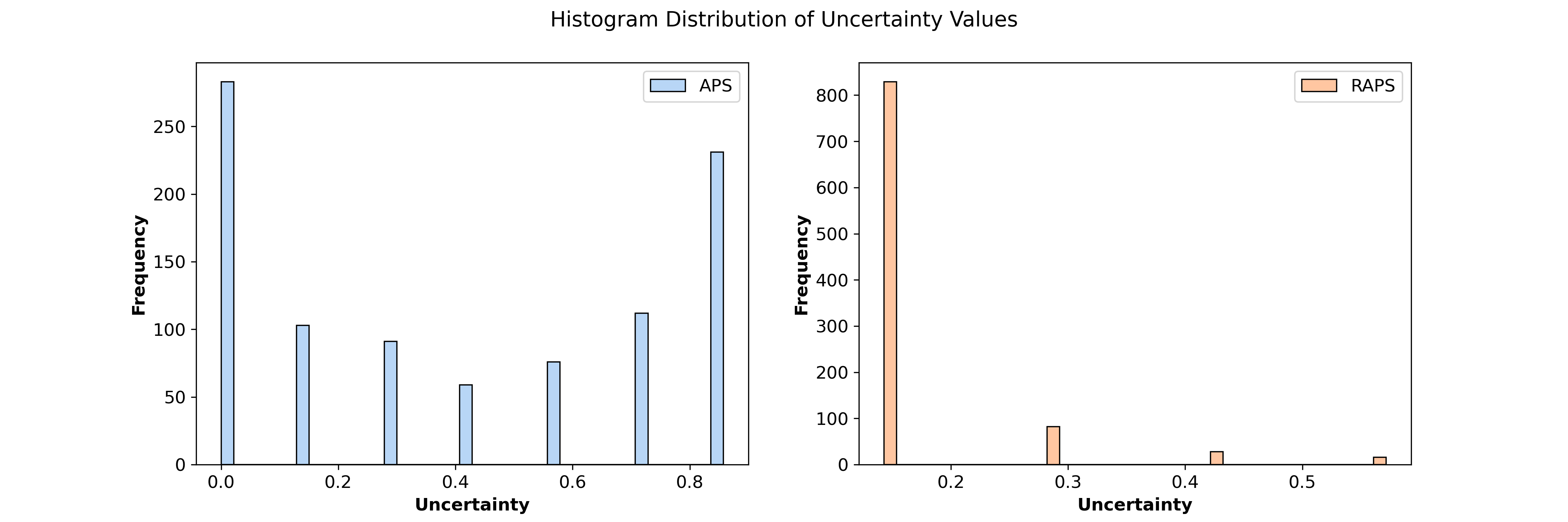
(a) Correctly classified samples

(b) Wrongly classified samples

Figure 4: Comparing the effect of APS Vs. RAPS on uncertainty assignments for both correctly classified samples and misclassified samples.

3.4.2 Confidence Level

The confidence level ($1-\alpha$) is a user-defined parameter, representing the probability of predicting the true label within the generated prediction set. The value of $\alpha$ is also used to compute the empirical quantile that splits the output scores into conforming and nonconforming scores. According to Equation 8, increasing $\alpha$ reduces the value of the quantile. at $\alpha=1.0$, the value of the quantile is $0$, hence the prediction set will produce empty sets of predictions. To further investigate the impact of increasing the value of $\alpha$, we examined the algorithm’s uncertainty assignment through the samples of misclassified data. As illustrated in Figure 5, it is evident that CP assigns high uncertainty values to a higher count of samples at $\alpha=0.1$. This is an expected behavior as the samples are wrongly classified, and hence they belong to the uncertain category. As the value of $\alpha$ increases, and the quantile value decreases, leading to a reduction in the number of samples generated with high uncertainty. Consequently, the count of certain samples increases, and eventually, those samples turn into empty prediction sets at higher $\alpha$ values.

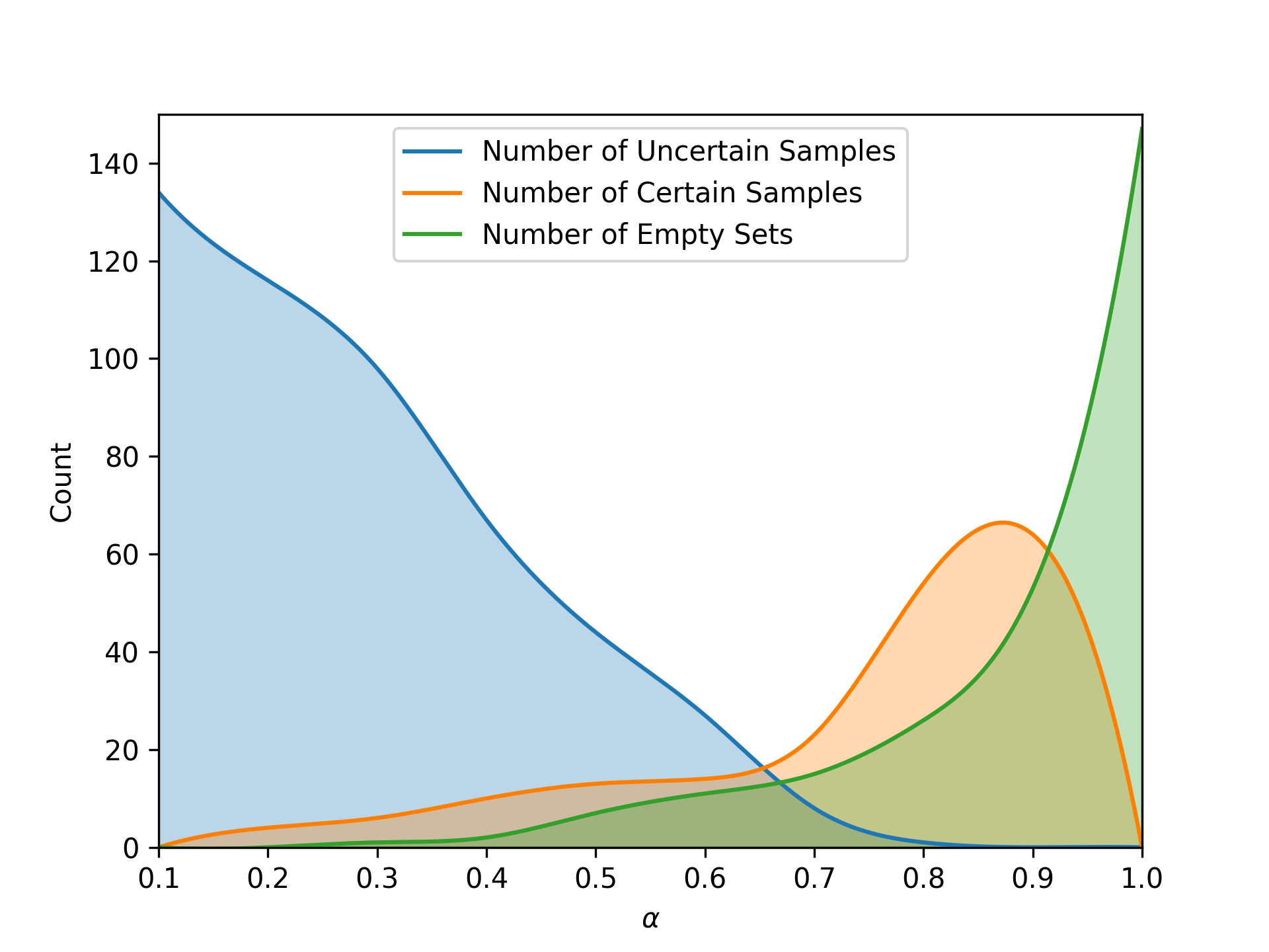
Figure 5: The relationship between the size of the calibration set and the empirical coverage of conformal prediction algorithm

3.4.3 Calibration set size

Varying the calibration set size has an immediate effect on the desired coverage. While conformal prediction guarantees coverage on an average runs on a calibration set, even if the number of samples used in the calibration data is small [29], It is however recommended to use a high number of samples in the calibration data to overcome any fluctuation in coverage and achieve stable performance. The effect of varying the calibration set size is illustrated in Figure 6, where it can be concluded that increasing the number of samples in the calibration size improves the empirical coverage achieved by the CP algorithm.

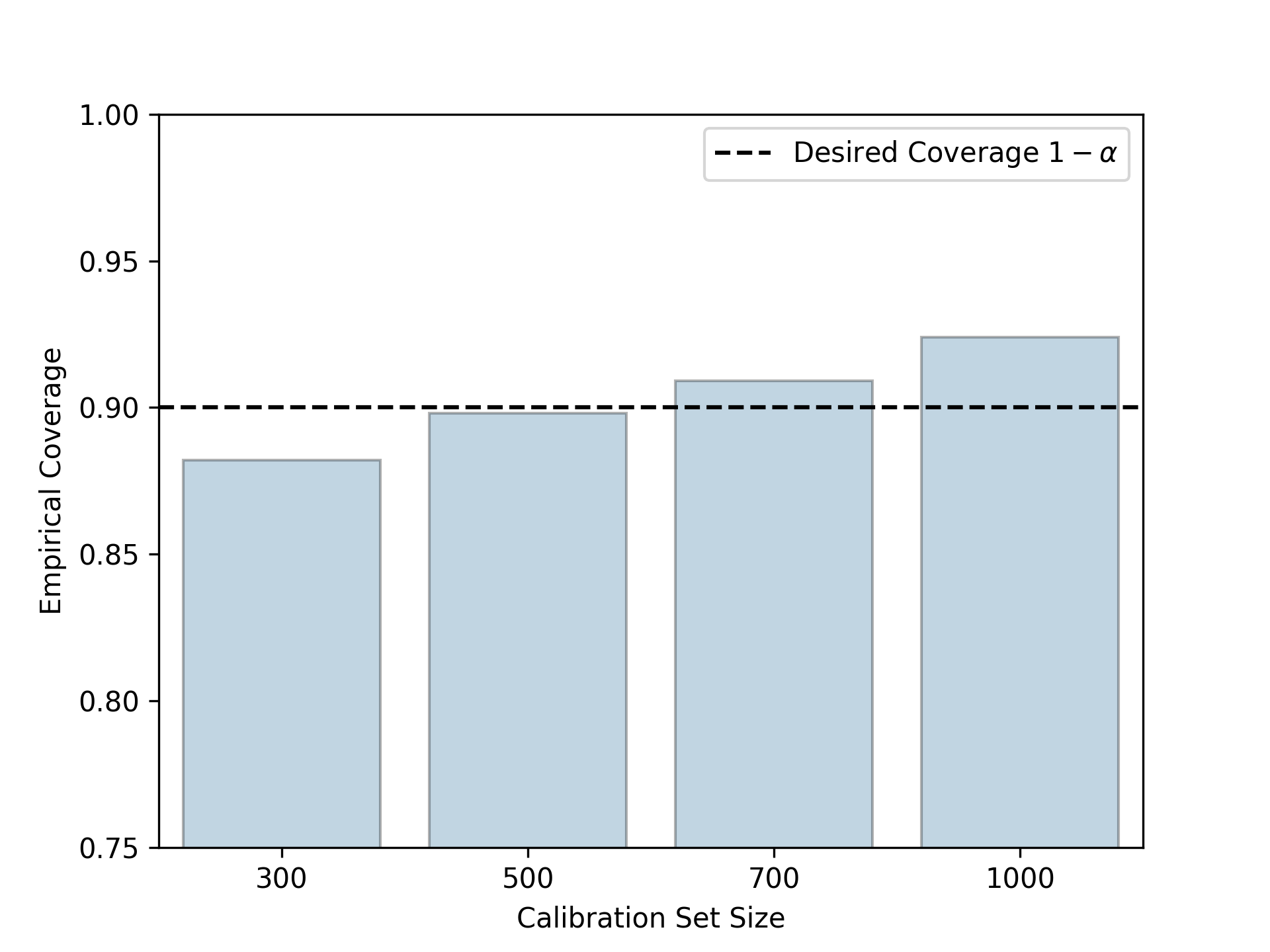
Figure 6: The relationship between the size of the calibration set and the empirical coverage of conformal prediction algorithm

3.5 Uncertainty Quantification with Out-of-Distribution Data

To assess the performance of the three uncertainty quantification methods, Out-of-Distribution (OOD) data is used for testing. OOD is a term that is generally used to refer to the distribution mismatch between the source domain (training data) and the target domain (inferencing data) [30, 31]. Generally, there are two categories of distributional shifts categorized based on the source of discrepancy: semantic shift, where the labels of the target data are different than the source data, and covariate shift, where shifts occur in the input domain, but labels remain unchanged.

In the context of skin lesion classification, we have selected the Dermofit Image Library (DMF) [32] dataset to evaluate the performance of uncertainty quantification algorithms. The DMF dataset contains images from real patients, featuring seven different types of skin lesions. Notably, these lesion types align with those found in the HAM10000 dataset, which was utilized to train the core model. Despite having similar labels for both datasets, each dataset is captured using different medical devices in distinct facilities. This divergence in settings introduces a covariate shift in the distribution of both datasets, presenting a noteworthy challenge for the underlying model. The distribution shift is visualized through a dimensionality reduction t-SNE plot of both datasets, as depicted in Figure 7.

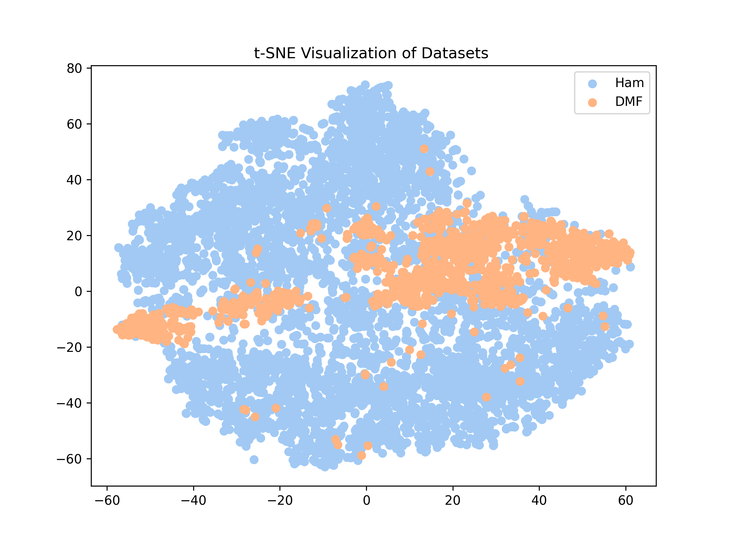
Figure 7: A visualization of the distribution of the HAM10000 and DMF dataset through the t-SNE dimensionailty reduction method.

The assigned uncertainty values during inference are recorded to analyze the reaction of each method to shifted data. The uncertainty distributions are shown in Figure 8. Ideally, high uncertainty values should be assigned to samples drawn from distributions different from those used during training. Figure 8 reveals that MCD exhibits inferior performance compared to both EDL and CP. While EDL effectively assigns high uncertainty values to a larger number of samples, CP achieves the best overall performance, where all the samples are assigned a high uncertainty value, indicating that the network is highly uncertain with the predictions.

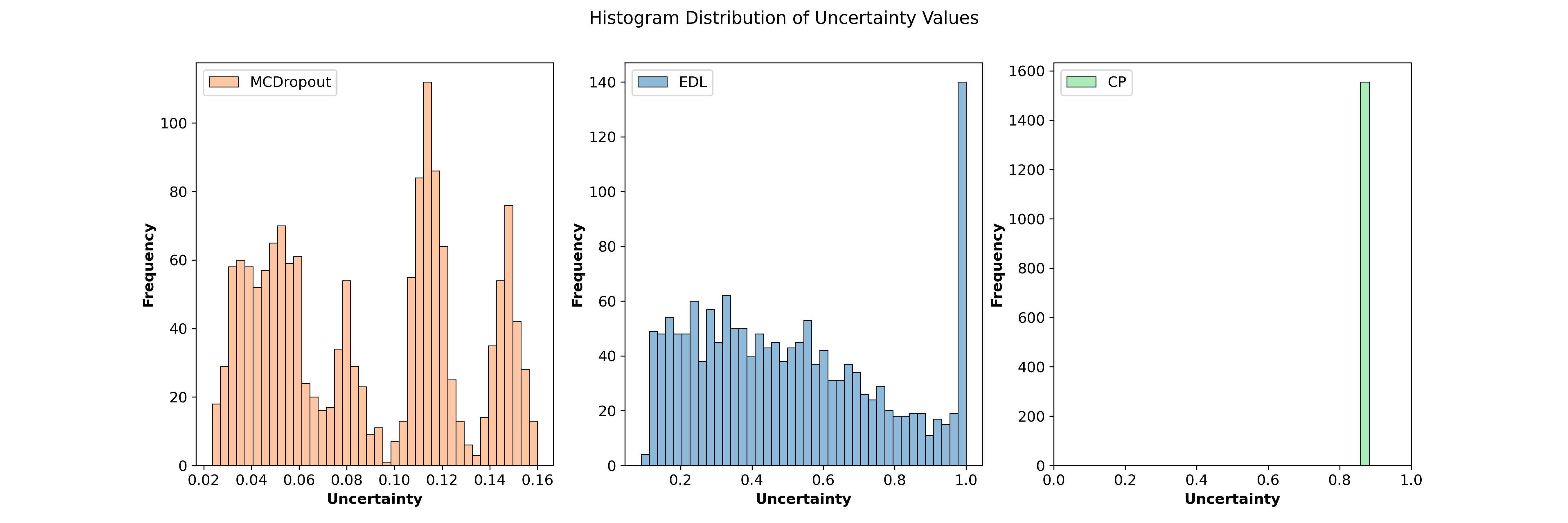
Figure 8: Histogram distribution of uncertainty estimations by Monte Carlo dropout, evidential deep learning, and conformal prediction algorithms. Dataset with covariate shift is used to assess the performance of the three methods.

4 Conclusion

This paper provides a comprehensive analysis of three uncertainty quantification techniques applied in the field of skin lesion medical image classification: Monte Carlo dropout, evidential deep learning, and conformal prediction. The performance of these methods is compared both qualitatively and quantitatively under various experimental conditions, to evaluate their effectiveness in quantifying uncertainty for a safety-critical application.

CP stands out as an emerging method that provides a robust and straightforward approach to quantifying predictive uncertainty. CP generates sets of predictions, where larger sets indicate higher uncertainty and vice versa. Experimental results demonstrate CP’s robustness when evaluated on correctly classified examples, showcasing its ability to generate varying levels of uncertainties that adapt to the difficulty of a given example. Notably, CP maintains consistent performance when assessed on wrongly classified examples, assigning higher uncertainty values compared to correctly classified samples. In contrast, both MCD and EDL lack these properties, leading to a superior performance of CP, as indicated in the comparative results. From an implementation point of view, CP offers lighter and more straightforward requirements compared to EDL or MCD. Unlike EDL, there is no need to retrain the core network, and unlike MCD, there is no requirement to modify the architecture. CP only requires the holdout of a dataset portion for calibration. Consequently, the method remains both model and dataset-agnostic.

In CP, the assumption that the calibration dataset is drawn from an independent and identical distribution (i.i.d) as the training dataset poses a limitation, particularly in real-world scenarios where models encounter diverse data. This assumption becomes restrictive as models are exposed to a broad spectrum of data, making the i.i.d assumption challenging to consistently uphold. While the reported results obtained from the OOD experiment showcase superior CP performance compared to other methods, it’s noteworthy that the testing dataset used doesn’t exhibit significant diversity from the training dataset. This limitation prompts consideration for future research directions, emphasizing the exploration of domain adaptation and generalization techniques to enhance model performance under domain shifts.

References

- [1] J. Fayyad, M. A. Jaradat, D. Gruyer, H. Najjaran, Deep learning sensor fusion for autonomous vehicle perception and localization: A review, Sensors 20 (15) (2020) 4220.
- [2] V. Wiley, T. Lucas, Computer vision and image processing: a paper review, International Journal of Artificial Intelligence Research 2 (1) (2018) 29–36.
- [3] S. Alijani, J. Tanha, L. Mohammadkhanli, An ensemble of deep learning algorithms for popularity prediction of flickr images, Multimedia Tools and Applications 81 (3) (2022) 3253–3274.
- [4] A. Salari, A. Djavadifar, X. Liu, H. Najjaran, Object recognition datasets and challenges: A review, Neurocomputing 495 (2022) 129–152.
- [5] X. X. Zhu, D. Tuia, L. Mou, G.-S. Xia, L. Zhang, F. Xu, F. Fraundorfer, Deep learning in remote sensing: A comprehensive review and list of resources, IEEE geoscience and remote sensing magazine 5 (4) (2017) 8–36.
- [6] B. Lambert, F. Forbes, A. Tucholka, S. Doyle, H. Dehaene, M. Dojat, Trustworthy clinical ai solutions: a unified review of uncertainty quantification in deep learning models for medical image analysis, arXiv preprint arXiv:2210.03736 (2022).
- [7] J. Fayyad, Out-of-distribution detection using inter-level features of deep neural networks, Ph.D. thesis, University of British Columbia (2023).
- [8] F. C. Ghesu, B. Georgescu, A. Mansoor, Y. Yoo, E. Gibson, R. Vishwanath, A. Balachandran, J. M. Balter, Y. Cao, R. Singh, et al., Quantifying and leveraging predictive uncertainty for medical image assessment, Medical Image Analysis 68 (2021) 101855.
- [9] M. Abdar, F. Pourpanah, S. Hussain, D. Rezazadegan, L. Liu, M. Ghavamzadeh, P. Fieguth, X. Cao, A. Khosravi, U. R. Acharya, et al., A review of uncertainty quantification in deep learning: Techniques, applications and challenges, Information fusion 76 (2021) 243–297.
- [10] H. Wei, R. Xie, H. Cheng, L. Feng, B. An, Y. Li, Mitigating neural network overconfidence with logit normalization, in: International Conference on Machine Learning, PMLR, 2022, pp. 23631–23644.
- [11] C. Guo, G. Pleiss, Y. Sun, K. Q. Weinberger, On calibration of modern neural networks, in: International conference on machine learning, PMLR, 2017, pp. 1321–1330.
- [12] M. Sensoy, L. Kaplan, M. Kandemir, Evidential deep learning to quantify classification uncertainty, Advances in Neural Information Processing Systems 31 (2018).
- [13] A. Malinin, M. Gales, Predictive uncertainty estimation via prior networks, Advances in neural information processing systems 31 (2018).
- [14] I. Kononenko, Bayesian neural networks, Biological Cybernetics 61 (5) (1989) 361–370.
- [15] D. M. Blei, A. Kucukelbir, J. D. McAuliffe, Variational inference: A review for statisticians, Journal of the American statistical Association 112 (518) (2017) 859–877.
- [16] S. Brooks, Markov chain monte carlo method and its application, Journal of the royal statistical society: series D (the Statistician) 47 (1) (1998) 69–100.
- [17] B. Lakshminarayanan, A. Pritzel, C. Blundell, Simple and scalable predictive uncertainty estimation using deep ensembles, Advances in neural information processing systems 30 (2017).
- [18] G. Shafer, V. Vovk, A tutorial on conformal prediction., Journal of Machine Learning Research 9 (3) (2008).
- [19] V. Vovk, A. Gammerman, G. Shafer, Algorithmic learning in a random world, Vol. 29, Springer.
- [20] A. Angelopoulos, S. Bates, J. Malik, M. I. Jordan, Uncertainty sets for image classifiers using conformal prediction, arXiv preprint arXiv:2009.14193 (2020).
- [21] A. N. Angelopoulos, A. P. Kohli, S. Bates, M. Jordan, J. Malik, T. Alshaabi, S. Upadhyayula, Y. Romano, Image-to-image regression with distribution-free uncertainty quantification and applications in imaging, in: International Conference on Machine Learning, PMLR, 2022, pp. 717–730.
- [22] W. He, Z. Jiang, A survey on uncertainty quantification methods for deep neural networks: An uncertainty source perspective, arXiv preprint arXiv:2302.13425 (2023).
- [23] J. Caldeira, B. Nord, Deeply uncertain: comparing methods of uncertainty quantification in deep learning algorithms, Machine Learning: Science and Technology 2 (1) (2020) 015002.
- [24] Y. Gal, Z. Ghahramani, Dropout as a bayesian approximation: Representing model uncertainty in deep learning, in: international conference on machine learning, PMLR, 2016, pp. 1050–1059.
- [25] D. Ulmer, G. Cinà, Know your limits: Monotonicity & softmax make neural classifiers overconfident on ood data, arXiv preprint arXiv:2012.05329 (2020).
- [26] G. Shafer, Dempster-shafer theory, Encyclopedia of artificial intelligence 1 (1992) 330–331.
- [27] P. Tschandl, C. Rosendahl, H. Kittler, The ham10000 dataset, a large collection of multi-source dermatoscopic images of common pigmented skin lesions, Scientific data 5 (1) (2018) 1–9.
- [28] K. He, X. Zhang, S. Ren, J. Sun, Deep residual learning for image recognition, in: Proceedings of the IEEE conference on computer vision and pattern recognition, 2016, pp. 770–778.
- [29] A. N. Angelopoulos, S. Bates, A gentle introduction to conformal prediction and distribution-free uncertainty quantification, arXiv preprint arXiv:2107.07511 (2021).
- [30] Z. Shen, J. Liu, Y. He, X. Zhang, R. Xu, H. Yu, P. Cui, Towards out-of-distribution generalization: A survey, arXiv preprint arXiv:2108.13624 (2021).
- [31] J. Yang, K. Zhou, Y. Li, Z. Liu, Generalized out-of-distribution detection: A survey, arXiv preprint arXiv:2110.11334 (2021).
- [32] L. Ballerini, R. B. Fisher, B. Aldridge, J. Rees, A color and texture based hierarchical k-nn approach to the classification of non-melanoma skin lesions, Color medical image analysis (2013) 63–86.