The Pfaffian Structure of CFN Phylogenetic Networks

Abstract.

Algebraic techniques in phylogenetics have historically been successful at proving identifiability results and have also led to novel reconstruction algorithms. In this paper, we study the ideal of phylogenetic invariants of the Cavender-Farris-Neyman (CFN) model on a phylogenetic network with the goal of providing a description of the invariants which is useful for network inference. It was previously shown that to characterize the invariants of any level-1 network, it suffices to understand all sunlet networks, which are those consisting of a single cycle with a leaf adjacent to each cycle vertex. We show that the parameterization of an affine open patch of the CFN sunlet model, which intersects the probability simplex factors through the space of skew-symmetric matrices via Pfaffians. We then show that this affine patch is isomorphic to a determinantal variety and give an explicit Gröbner basis for the associated ideal, which involves only polynomially many coordinates. Lastly, we show that sunlet networks with at least 6 leaves are identifiable using only these polynomials and run extensive simulations, which show that these polynomials can be used to accurately infer the correct network from DNA sequence data.

1. Introduction

Phylogenetic networks are directed acyclic graphs that are used to represent the evolutionary history of a set of species where reticulation events, such as hybridization or horizontal gene transfer, may have occurred. A phylogenetic network is typically equipped with a parametric statistical model of evolution, which enables phylogenetic analyses and network inference from genome data. One recent approach to network inference is rooted in computational algebraic geometry. For example, algebraic methods have recently been used to establish identifiability for several classes of network models [2, 5, 14, 15, 17, 19] and for network inference [1, 6, 21, 30]. In particular, [6] and [21] investigate using algebraic techniques to infer networks from molecular sequence data. Most algebraic results on identifiability or inference utilize the phylogenetic invariants of the model, which are polynomials that vanish on every distribution in the model; thus, one common problem for any statistical model associated with a phylogenetic network is to characterize the set of invariants of the model.

While ideals of phylogenetic invariants are useful for different statistical inference problems, very little is known about these ideals for network-based Markov models, or equivalently, displayed tree models. In [8] a partial description of the invariants for equivariant models is given but these invariants do not suffice to reconstruct a network entirely. One natural place to begin is the study of group-based Markov models, since the discrete Fourier transform can be used to greatly simplify the parameterization [11, 18], which makes it much more amenable to study from an algebraic perspective. This is further evidenced by the fact that invariants of group-based models for trees are completely characterized [27], but for many other equivariant models, they are still unknown [4]. The study of the invariants for group-based models on networks was started in [15] with a focus on identifiability. More recently, in [10], the authors show that the invariants of a group-based model on level-1 phylogenetic networks can be completely determined if the invariants of all sunlet networks are known. The authors then identified all quadratic invariants in the sunlet network ideal for the Cavendar-Farris-Neyman (CFN) model.

In this paper, we complete the study of the invariants of the CFN model on a sunlet network. In particular, we show that the parameterization of the CFN sunlet network model factors through the parameterization of the Pfaffians of a generic skew-symmetric matrix, allowing us to work with the model in a new coordinate system. While this is not directly related to the results in [20], it does provide another surprising link between Pfaffians and phylogenetics. The following theorem summarizes our main results.

Theorem.

Let $V_{n}\subseteq{\mathbb{P}}^{2^{n-1}-1}$ be the phylogenetic variety associated to the $n$-leaf sunlet network. Consider the statistically relevant affine open patch, $U=V_{n}\setminus\mathcal{H}$, of $V_{n}$ where $\mathcal{H}$ is the hyperplane given by the sum of the probability coordinates. Then:

1. $U$ embeds into the space of $n\times n$ skew symmetric matrices.

2. In these new coordinates, $U$ is a determinantal variety which is cut out by certain $2\times 2$ and $3\times 3$ minors of a generic skew-symmetric matrix $\Omega$.

We give an explicit characterization of the $2\times 2$ and $3\times 3$ minors that cut out $U$ in this new coordinate system and also show that these minors form a Gröbner basis for the vanishing ideal of $U$. We then show that the invariants of the original model in projective space can be obtained from our minors, along with the relations between the Pfaffians of a skew-symmetric matrix by homogenization and saturation. These results essentially give a complete description of the invariants of the CFN model. Lastly, we use this new description of the CFN model to show that sunlet networks with at least 6 leaves are identifiable and provide extensive simulations that show that it suffices to use these determinantal invariants for network inference.

The remainder of this paper is organized as follows. In Section 2, we review background material on phylogenetic networks, Markov models, and Pfaffians. In Section 3 we show that the parameterization of the sunlet network model factors through the parameterization of the Pfaffians of a skew-symmetric matrix and utilize this to give a complete description of the invariants of the statistically relevant patch of the model in a new coordinate system. In Section 4 we prove that sunlet networks with at least 6 leaves are identifiable under the CFN model and then show that these invariants can be used to accurately infer the correct network from simulated DNA sequence data. Lastly, in Appendix A, we give an alternative proof of the dimension of the variety and show that it is Cohen-Macaulay by finding a shelling of the Stanley-Reisner complex associated with its initial ideal.

2. Preliminaries

This section provides a brief overview of the Cavender-Farris-Neyman (CFN) model on phylogenetic trees and networks. We then provide some background on the structure of the vanishing ideal of the CFN model associated to a phylogenetic tree, which was characterized in [27], and review the multigrading described in [10] in which the sunlet network ideals are homogeneous.

2.1. Phylogenetic Networks

In this subsection, we provide some brief background on phylogenetic networks. Our notation and terminology are adapted from [10, 15]. For more information on the combinatorics of networks, we refer the reader to [16, 25].

A phylogenetic network on $n$ leaves is a rooted, directed, acyclic graph, where the root vertex is a distinguished vertex of out-degree two, and all other vertices have either in-degree one and out-degree two (these are called tree vertices), in-degree two and out-degree one (these are called reticulation vertices), or in-degree 1 (these are called leaf vertices). The set of leaf vertices is identified with the set of integers $[n]$. Edges directed into a reticulation vertex are called reticulation edges, and all other edges are called tree edges. In this paper, we will focus on the Cavender-Farris-Neyman model, which is group-based and thus time-reversible. This means that it is impossible to identify the location of the root under these models so we restrict our attention to the underlying semi-directed network structure of the phylogenetic network. The underlying semi-directed network is a mixed graph obtained by suppressing the root and undirecting all tree edges in the network. The reticulation edges remain directed into the reticulation vertex. Since the reticulation edges are implicitly directed into the reticulation vertex, we typically omit the arrows when drawing semi-directed networks. This is illustrated in Figure 1.

Figure 1. A four-leaf, level-1 network pictured on the left with all edges directed away from the root. In the center is the associated semidirected network obtained by suppressing the root and undirecting all tree edges. The edges are implicitly assumed to be directed into the vertex adjacent to the leaf $1$, which is the reticulation vertex. On the left, a level-1 network with $2$ connected components is pictured.

The definition of networks above is very general and allows for an extremely wide array of structures, making it difficult to analyze or study general networks. This means that subclasses of networks are often studied instead. In this paper, we restrict to the subclass of level-1 networks which are networks with at most 1 cycle in each 2-connected component. This class of networks is particularly nice since they can be formed by gluing trees and sunlet networks of potentially different sizes together along leaves.

Definition 2.1.

A $n$-sunlet network is a semi-directed network with one reticulation vertex and whose underlying graph is obtained by adding a pendant edge to every vertex of a $n$-cycle. We denote with $\mathcal{S}_{n}$ the $n$-sunlet network with reticulation vertex adjacent to the leaf 1 and the other leaves labeled circularly from 1.

This class of networks was first introduced in [15] and was further studied in [10]. Throughout this paper, we will focus primarily on sunlet networks since the invariants of any level-1 network under the CFN model (or indeed, any group-based model) can be determined if the invariants of all $n$-leaf sunlet networks are known [15, 10].

2.2. Phylogenetic Markov models and the Cavender-Farris-Neyman Model

In this subsection, we briefly describe the phylogenetic Markov models with a particular focus on the Cavender-Farris-Neyman (CFN) model. We begin with phylogenetic Markov models on trees since they will be the main ingredient for constructing models on networks.

A $\kappa$-state Markov model on a $n$-leaf phylogenetic tree $\mathcal{T}$ yields a distribution on all possible states that can be jointly observed at the leaves of $\mathcal{T}$. These states are also called marginal characters, and are often interpreted as being the possible columns representing a single site in aligned sequence data. For example, when $\kappa=4$ and the state space is the nucleic acids $\{\rm{A,G,C,T}\}$, each joint state is a column that can appear in an alignment of DNA sequence data.

The distribution of joint states is produced by associating a $\kappa$-state random variable $X_{v}$ to each vertex $v$ of $\mathcal{T}$ and a $\kappa\times\kappa$ transition matrix $M^{e}$ to each directed edge $(u,v)$ such that $M_{i,j}^{e}=P(X_{v}=j|X_{u}=i)$. Lastly, associate a distribution $\pi$ to the root $\rho$ of $\mathcal{T}$. Observe that this means the state space of each random variable is naturally $[\kappa]=\{1,\ldots,\kappa\}$. Then the probability of observing a joint state $(x_{1},\ldots,x_{n})\in[\kappa]^{n}$ is

$$p_{x_{1}x_{2}\ldots x_{n}}:=P(X_{1}=x_{1},\ldots,X_{n}=x_{n})\leavevmode\nobreak\ =\sum_{j\in[\kappa]^{Int(\mathcal{T})}}\pi_{j_{\rho}}\prod_{(u,v)\in E(\mathcal{T})}M_{j_{u},j_{v}}^{(u,v)},$$

where $X_{1},\ldots,X_{n}$ are the random variables associated to the leaves of $\mathcal{T}$. Observe that the joint distribution $p=(p_{x_{1}x_{2}\ldots x_{n}}\leavevmode\nobreak\ |\leavevmode\nobreak\ (x_{1},\ldots,x_{n})\in[\kappa]^{n})$ of $(X_{1},\ldots X_{n})$ is given by polynomials in the entries of $\pi$ and the $M^{e}$. In other words, the model can be thought of as the image of a polynomial map

$$\varphi_{\mathcal{T}}\leavevmode\nobreak\ :\leavevmode\nobreak\ \Theta_{\mathcal{T}} \to\Delta_{\kappa^{n}-1}=\{p\in{\mathbb{R}}^{\kappa^{n}}\leavevmode\nobreak\ |\leavevmode\nobreak\ \sum_{(x_{1},\ldots,x_{n})\in[\kappa]^{n}}p_{x_{1}x_{2}\ldots x_{n}}=1\leavevmode\nobreak\ \mathrm{and}\leavevmode\nobreak\ p_{x_{1}x_{2}\ldots x_{n}}\geq 0\}$$

$$(\pi,M^{e}) \mapsto\varphi_{\mathcal{T}}(\pi,M^{e})=\sum_{j\in[\kappa]^{Int(\mathcal{T})}}\pi_{j_{\rho}}\prod_{(u,v)\in E(\mathcal{T})}M_{j_{u},j_{v}}^{(u,v)}$$

where $\Theta_{\mathcal{T}}$ is the stochastic parameter space of the model which consists of all possible tuples $(\pi,M^{e}\leavevmode\nobreak\ |\leavevmode\nobreak\ e\in E(\mathcal{T}))$ of root distributions and transition matrices. This means that tools from commutative algebra and algebraic geometry can be used to study the phylogenetic model $M_{\mathcal{T}}=\operatorname{image}(\varphi_{\mathcal{T}})$ which is the main idea behind algebraic statistics [29]. In particular, algebraic tools can be used to determine invariants of the model, prove identifiability results, and can even yield algorithms for network inference as we will see throughout the remainder of this paper.

Phylogenetic Markov models for trees naturally induce a model on phylogenetic networks in the following way. Let $\mathcal{N}$ be a phylogenetic network with reticulation vertices $v_{1},\dots v_{m}$, and let $e_{i}^{0}$ and $e_{i}^{1}$ be the reticulation edges adjacent to $v_{i}$. Associate a transition matrix to each edge of $\mathcal{N}$. Independently at random delete $e_{i}^{0}$ with probability $\lambda_{i}$ and otherwise delete $e_{i}^{1}$ and record which edge is deleted with a vector $\sigma\in\{0,1\}^{m}$ where $\sigma_{i}=0$ indicates that edge $e_{i}^{0}$ was deleted. Each $\sigma$ corresponds to a different tree $T_{\sigma}$, which corresponds to the different possible lineages for the species at the leaves of the network. Then the parameterization $\varphi_{\mathcal{N}}$ is given by

$$\varphi_{\mathcal{N}}=\sum_{\sigma\in\{0,1\}^{m}}\left(\prod_{i=1}^{m}\lambda_{i}^{1-\sigma_{i}}(1-\lambda_{i})^{\sigma_{i}}\right)\varphi_{\mathcal{T}_{\sigma}}$$ (2.1)

where $\varphi_{\mathcal{T}_{\sigma}}$ is the parameterization corresponding to the tree $\mathcal{T}_{\sigma}$ with transition matrices inherited from the original network $\mathcal{N}$. The network model is quite similar to a mixture model; however, the parameters on each tree ${\mathcal{T}_{\sigma}}$ are highly dependent since they are all inherited from the original network, whereas in a mixture model, the parameters on each tree are independent.

The model described above, with no restrictions on root distributions or transition matrices, is called the general Markov model. This has received extensive study for phylogenetic trees, but even in that simpler setting, it can be difficult to analyze [3, 4]. Often, simpler models of DNA evolution are specified by requiring that the transition matrices satisfy additional constraints. One well-studied family of models for phylogenetic trees is the following.

Definition 2.2.

Let $G$ be a finite abelian group of order $\kappa$ and $\mathcal{T}$ a rooted binary tree. Then a group-based model on $\mathcal{T}$ is a phylogenetic Markov model on $\mathcal{T}$ such that for each transition matrix $M^{e}$, there exists a function $f_{e}:G\to{\mathbb{R}}$ such that $M_{g,h}^{e}=f(g-h)$.

Many well-known phylogenetic models are group-based, such as the Jukes-Cantor, Kimura 2-Parameter, and Kimura 3-Parameter models and, of course, the Cavender-Farris-Neyman (CFN) model, which is the main focus of this paper. Group-based models are particularly amenable to study from an algebraic perspective since they allow for a linear change of coordinates, which vastly simplifies the parameterization of the model. This change of coordinates is called the discrete Fourier transform and was first applied to phylogenetic models in [11, 18]. After applying this change of coordinates, the resulting coordinates are typically called the Fourier coordinates and are denoted by $q_{g_{1}g_{2}\ldots g_{n}}$ for $g_{1},\ldots,g_{n}\in G$, where we now identify $G$ with the state space of the model. In what follows, we define the parameterization for the CFN model after this change of coordinates and refer the reader to [25, 29] for more detailed information.

The CFN model is a 2-state group-based model associated with the group ${\mathbb{Z}}/2{\mathbb{Z}}$. In the Fourier coordinates, it is parameterized using the splits of the tree $\mathcal{T}$. Each edge $e\in\mathcal{T}$ has an associated split $A_{e}|B_{e}$, which is the partition of the leaf set of $\mathcal{T}$ obtained by deleting the edge $e$. To parameterize the CFN model in the Fourier coordinates, associate parameters $a_{g}^{e}$ for each $g\in{\mathbb{Z}}/2{\mathbb{Z}}$ and edge $e$. The parameterization of the model is then given by

$$q_{g_{1}\ldots g_{n}}=\begin{cases}\prod_{e\in E(\mathcal{T})}a_{\sum_{i\in A_{e}}g_{i}}^{e}&\mbox{ if }\sum_{i\in[n]}g_{i}=0\\ 0&\mbox{ otherwise}\end{cases}$$ (2.2)

Since this change of coordinates is linear, it naturally extends to networks as well. We end this subsection with the following example illustrating this new parameterization for both trees and networks.

(a) $\mathcal{S}_{4}$

(b) $\mathcal{T}_{0}$

(c) $\mathcal{T}_{1}$

Figure 2. The four leaf sunlet network $\mathcal{S}_{4}$ and the two trees $\mathcal{T}_{0}$ and $\mathcal{T}_{1}$ that are obtained by deleting the reticulation edges $e_{8}$ and $e_{5}$ respectively.

Example 2.3.

Let $\mathcal{S}_{4}$ be the 4-sunlet pictured in Figure 2. The two trees $\mathcal{T}_{0}$ and $\mathcal{T}_{1}$ which are pictured to the right in Figure 2 are obtained from $\mathcal{S}_{4}$ by deleting the reticulation edges $e_{8}$ and $e_{5}$ respectively. The parameterization is given by $\varphi_{\mathcal{S}_{4}}=\lambda\varphi_{\mathcal{T}_{0}}+(1-\lambda)\varphi_{\mathcal{T}_{1}}$, where in the Fourier coordinates $\varphi_{\mathcal{T}_{0}}$ and $\varphi_{\mathcal{T}_{1}}$ are given by Equation 2.2. Explicitly, we have

$$q_{g_{1}g_{2}g_{3}g_{4}}=\begin{cases}\lambda a_{g_{1}}^{1}a_{g_{2}}^{2}a_{g_{3}}^{3}a_{g_{4}}^{4}a_{g_{1}}^{5}a_{g_{1}+g_{2}}^{6}a_{g_{4}}^{7}+(1-\lambda)a_{g_{1}}^{1}a_{g_{2}}^{2}a_{g_{3}}^{3}a_{g_{4}}^{4}a_{g_{3}}^{6}a_{g_{1}+g_{4}}^{7}a_{g_{1}}^{8}&\mbox{ if }\sum_{i\in[4]}g_{i}=0\\ 0&\mbox{ otherwise}\end{cases}$$

Here, the first term comes from the parameterization $\varphi_{\mathcal{T}_{0}}$, and the second term comes from $\varphi_{\mathcal{T}_{1}}$. Observe that for all $g$ in $G$ the parameters $a_{g}^{5}$ and $a_{g}^{8}$ only occur in the first and second terms respectively, since they correspond to the deleted reticulation edges. This means we can make the substitution $\lambda a_{g}^{5}\mapsto a_{g}^{5}$ and $(1-\lambda)a_{g}^{8}\mapsto a_{g}^{8}$ without changing the parameterization of the model as was noted in [15]. So, for example, after this change the coordinate $q_{1001}$ is given by

$$q_{1001}=a_{1}^{1}a_{0}^{2}a_{0}^{3}a_{1}^{4}a_{1}^{5}a_{1}^{6}a_{1}^{7}+a_{1}^{1}a_{0}^{2}a_{0}^{3}a_{1}^{4}a_{0}^{6}a_{0}^{7}a_{1}^{8}=a_{1}^{1}a_{0}^{2}a_{0}^{3}a_{1}^{4}(a_{1}^{5}a_{1}^{6}a_{1}^{7}+a_{0}^{6}a_{0}^{7}a_{1}^{8}).$$

∎

2.3. Phylogenetic Invariants and Algebraic Statistics

In this subsection, we give a brief overview of some algebraic structures which we will need to describe the invariants for the CFN model on trees [27] and the quadratic invariants for the CFN mdoel on networks that were found in [10]. Both of these characterizations will be key in the construction of our alternative parameterization of the CFN sunlet model in Section 3 and our description of all of the invariants in this new coordinate system. For additional information on the algebraic concepts discussed below, we refer the reader to [9, 29].

As discussed in the previous section, all phylogenetic Markov models on a tree or a network can be thought of as the image of a polynomial map $\varphi$. A fundamental problem concerning any such phylogenetic model is to determine the ideal of phylogenetic invariants, also called the vanishing ideal of the model.

Definition 2.4.

Let $\mathbb{K}$ be a field and $S\subseteq\mathbb{K}^{m}$. The vanishing ideal of $S$ is the set of multivariate polynomials

$$\mathcal{I}(S):=\{f\in\mathbb{K}[x_{1},\ldots,x_{m}]\leavevmode\nobreak\ |\leavevmode\nobreak\ f(s)=0\leavevmode\nobreak\ \mbox{for all}\leavevmode\nobreak\ s\in S\}.$$

For instance, if $\varphi=\varphi_{\mathcal{T}}$ is the parameterization of the CFN model on a tree $\mathcal{T}$ in the Fourier coordinates, then the ideal of phylogenetic invariants is $I_{\mathcal{T}}=\mathcal{I}(\operatorname{image}(\varphi_{\mathcal{T}}))$. This means that invariants are just multivariate polynomials in the Fourier coordinates $q_{g_{1}\ldots q_{n}}$, which evaluate to zero on every point in the image of the map $\varphi_{\mathcal{T}}$. We can similarly define the ideal of invariants for a network as $I_{\mathcal{N}}=\mathcal{I}(\operatorname{image}(\varphi_{\mathcal{N}}))$. Every ideal $I$ of a polynomial ring $\mathbb{K}[x_{1},\ldots,x_{m}]$ has an associated affine algebraic variety which is

$$\mathcal{V}(I)=\{s\in\mathbb{K}^{m}\leavevmode\nobreak\ |\leavevmode\nobreak\ f(s)=0\leavevmode\nobreak\ \mbox{for all}\leavevmode\nobreak\ f\in I\}.$$

When $I$ is the vanishing ideal of a set $S$ then $\mathcal{V}(I)$ is the Zariski closure of $S$. The phylogenetic variety of a tree $\mathcal{T}$ is $\mathcal{V}(I_{\mathcal{T}})$ and similarly for networks. This set essentially consists of all points that come from ignoring the stochastic restrictions of the parameter space $\Theta_{\mathcal{T}}$ and extending $\varphi_{\mathcal{T}}$ to a complex polynomial map.

Remark 2.5.

While we have defined the phylogenetic variety as an affine variety, when the model is group-based, it is common to think of these as projective varieties. The CFN parameterization, for example, can be thought of as the image of a map of the form below:

$$\prod_{e\in E(\mathcal{T})}{\mathbb{P}}^{1}\to{\mathbb{P}}^{2^{n-1}-1}$$

where the homogeneous coordinates of each ${\mathbb{P}}^{1}$ are $[a_{0}^{e}:a_{1}^{e}]$, and the projective coordinates of ${\mathbb{P}}^{2^{n-1}-1}$ are the Fourier coordinates. In Section 3, we will consider an affine open patch of this variety where $\sum_{g\in\{0,1\}^{n}}p_{g}=q_{00\dots 0}=1$.

The ideal $I_{T}$ for any tree $T$ under the CFN model was completely characterized by the following theorem from [27].

Theorem 2.6.

[27] Let $\mathcal{T}$ be a tree and $I_{\mathcal{T}}$ be the ideal of phylogenetic invariants of the CFN model. Then $I_{\mathcal{T}}$ is generated by the $2\times 2$ minors of the matrices $M_{0}^{A_{e}|B_{e}}$ and $M_{1}^{A_{e}|B_{e}}$ which correspond to all flattenings along internal edges $e$.

The following example illustrates this construction for a small tree.

Example 2.7.

Let $\mathcal{T}$ be the unrooted binary tree with 4 leaves whose only nontrivial split is split $A|B=12|34$. Then $I_{\mathcal{T}}$ is generated by the $2\times 2$ minors of the following matrices

$$M_{0}^{A|B}=\blockarray{ccc}&0011\\ \block{c(cc)}00q_{0000}q_{0011}\\ 11q_{1100}q_{1111}\\ \leavevmode\nobreak\ \leavevmode\nobreak\ \leavevmode\nobreak\ \leavevmode\nobreak\ \leavevmode\nobreak\ \leavevmode\nobreak\ \leavevmode\nobreak\ \leavevmode\nobreak\ M_{1}^{A|B}=\blockarray{ccc}&0110\\ \block{c(cc)}01q_{0101}q_{0110}\\ 10q_{1001}q_{1010}\\ .$$

So the ideal of phylogenetic invariants for $\mathcal{T}$ is $I_{\mathcal{T}}=\langle q_{0000}q_{1111}-q_{0011}q_{1100},\leavevmode\nobreak\ q_{0101}q_{1010}-q_{0110}q_{1001}\rangle$. ∎

In [10], the authors show that the invariants of any level-1 phylogenetic network under a group-based model can be determined from the invariants of phylogenetic trees and sunlet networks using the toric fiber product [28]. They then give a complete description of the quadratic invariants of the model and conjecture that the ideal $I_{\mathcal{S}_{n}}$ is generated by these quadratics. One key observation in this description of the invariants is that the parameterization $\varphi_{n}=\varphi_{\mathcal{S}_{n}}$ of the $n$-leaf sunlet network is homogeneous in the multigrading defined by

$$\deg(q_{g})=(1,g)\in{\mathbb{Z}}^{n+1},$$

where $g$ is treated as a $0/1$ integer vector instead of as a vector with ${\mathbb{Z}}/2{\mathbb{Z}}$ entries. In the next section, we will provide an alternate perspective on the ideal $I_{\mathcal{S}_{n}}$, which lets us describe the invariants of this model using determinantal constraints.

2.4. Pfaffians of Skew-Symmetric Matrices

In this subsection, we briefly remind the reader of some properties of the Pfaffian of a skew-symmetric matrix, which will be crucial in Section 3.

Definition 2.8.

Let $S_{n}$ be the symmetric group of order $n$, and $A$ an $n\times n$ skew-symmetric matrix where $n=2m$ for some integer $m>1$. The Pfaffian of $A$, denoted $\text{Pf}(A)$, is defined as

$$\text{Pf}(A)=\frac{1}{2^{m}m!}\sum_{\sigma\in S_{n}}\operatorname{sign}(\sigma)\prod_{1\leq j\leq m}a_{\sigma(2j-1),\sigma(2j)}.$$ (2.3)

The following proposition gives us two ways to compute the Pfaffian of a skew-symmetric matrix, the second of which will be of use to us in Section 3.

Proposition 2.9.

Let $A$ be a skew-symmetric matrix. Then

$$(\operatorname{Pf}(A))^{2}=\det(A).$$

Moreover, there is also a Laplace-like expansion for the Pfaffian. If $A$ is a $2n\times 2n$ skew-symmetric matrix, let $A_{ij}$ be the submatrix of $A$ where we delete both the $i^{\text{th}}$ and $j^{\text{th}}$ rows and columns of $A$. Then

$$\mathrm{Pf}(A)=\sum_{j=2}^{2n}(-1)^{j}a_{1,j}\mathrm{Pf}(A_{1j})$$

where $A=(a_{ij})$.

3. The Pfaffian Structure of CFN Network Ideals

In this section, we show that the parameterization of the CFN sunlet network model factors through the space of skew-symmetric matrices via the Pfaffian. We use this to provide an alternative parameterization of the CFN sunlet model and determine a Gröbner basis for the corresponding vanishing ideal. We begin with a motivating example when $n=4$.

Example 3.1.

The CFN phylogenetic variety of the 4-leaf sunlet network is cut out by a single quadratic in ${\mathbb{P}}^{7}$.

$$V_{4}=\mathcal{V}(q_{0000}q_{1111}-q_{0011}q_{1100}+q_{0101}q_{1010}-q_{0110}q_{1001})$$

Upon closer inspection, one might realize that this equation is exactly a homogenized relation among the sub-Pfaffians of a generic skew-symmetric matrix. Indeed, let $\Omega^{4}$ be the skew-symmetric matrix below.

$$\begin{pmatrix}0&x_{12}&x_{13}&x_{14}\\ -x_{12}&0&x_{23}&x_{24}\\ -x_{13}&-x_{23}&0&x_{34}\\ -x_{14}&-x_{24}&-x_{34}&0\end{pmatrix}$$

For a subset $S\subseteq[4]$ of even cardinality, we define $\Omega^{4}_{S}$ to be the matrix whose rows and columns are indexed by $S$, and we can compute their Pfaffians.

$$\mathrm{Pf}(\Omega^{4}_{\emptyset}) =1 \mathrm{Pf}(\Omega^{4}_{\{1,2\}}) =x_{12}$$

$$\mathrm{Pf}(\Omega^{4}_{\{1,3\}}) =x_{13} \mathrm{Pf}(\Omega^{4}_{\{1,4\}}) =x_{14}$$

$$\mathrm{Pf}(\Omega^{4}_{\{2,3\}}) =x_{23} \mathrm{Pf}(\Omega^{4}_{\{2,4\}}) =x_{24}$$

$$\mathrm{Pf}(\Omega^{4}_{\{3,4\}}) =x_{34} \mathrm{Pf}(\Omega^{4}) =x_{12}x_{34}-x_{13}x_{24}+x_{14}x_{23}$$

There is a single homogeneous relation among these given by

$$\mathrm{Pf}(\Omega^{4}_{\emptyset})\mathrm{Pf}(\Omega^{4})-\mathrm{Pf}(\Omega^{4}_{\{1,2\}})\mathrm{Pf}(\Omega^{4}_{\{3,4\}})+\mathrm{Pf}(\Omega^{4}_{\{1,3\}})\mathrm{Pf}(\Omega^{4}_{\{2,4\}})-\mathrm{Pf}(\Omega^{4}_{\{1,4\}})\mathrm{Pf}(\Omega^{4}_{\{2,3\}})=0$$

Now, if we identify $q_{g}$ with $\mathrm{Pf}(\Omega^{4}_{S})$ where $g$ is $\sum_{i\in S}e_{i}$, we see that the relation cutting out $\mathcal{S}_{4}$ is exactly the relation among the Pfaffians of a generic skew-symmetric matrix. Thus, one can identify the affine patch of $V_{4}$ where $q_{0000}\neq 0$ with the space of $4\times 4$ skew-symmetric matrices. ∎

The previous example is not a coincidence, and indeed we will show that a similar story holds for all $n\geq 4$. Consider the following three rings.

$$Q_{n} :=\mathbb{K}[q_{g}\leavevmode\nobreak\ |\leavevmode\nobreak\ g\in({\mathbb{Z}}/2{\mathbb{Z}})^{n}\text{ where }\sum_{i=1}^{n}g_{i}=0]$$

$$A_{n} :=\mathbb{K}[a^{i}\leavevmode\nobreak\ |\leavevmode\nobreak\ 1\leq i\leq 2n]$$

$$X_{n} :=\mathbb{K}[x_{ij}\leavevmode\nobreak\ |\leavevmode\nobreak\ 1\leq i<j\leq n]$$

In Fourier coordinates, the phylogenetic variety of the $n$-sunlet, denoted $V_{n}\subseteq{\mathbb{P}}^{2^{n-1}-1}$, is parameterized by $\prod_{i=1}^{2n}{\mathbb{P}}^{1}$, where the coordinates of each ${\mathbb{P}}^{1}$ are given by $[a^{i}_{0}:a^{i}_{1}]$. We can parameterize the affine open patch $V_{n}\setminus\mathcal{V}(q_{00\ldots 0})$ by $\prod_{i=1}^{2n}({\mathbb{P}}^{1}\setminus\mathcal{V}(a^{i}_{0}))$. This parameterization corresponds to the following ring homomorphism.

$$\varphi_{n}:Q_{n} \rightarrow A_{n}$$

$$q_{g} \mapsto\frac{1}{2}\prod_{\begin{subarray}{c}i\in[n]\\ g_{i}=1\end{subarray}}a^{i}\left(\prod_{\begin{subarray}{c}i\in[1,n-1]\\ \sum_{j=1}^{i}g_{j}=1\end{subarray}}a^{n+i}+\prod_{\begin{subarray}{c}i\in[2,n]\\ \sum_{j=2}^{i}g_{j}=1\end{subarray}}a^{n+i}\right).$$

We denote the kernel of $\varphi_{n}$ as $J_{n}$, so $V_{n}\setminus\mathcal{V}(q_{00\ldots 0})=\mathcal{V}(J_{n})$.

Remark 3.2.

We are more than justified in considering only this affine open patch of $V_{n}$. First of all, in the original probability coordinates, $q_{00\ldots 0}$ is equal to $\sum_{g\in({\mathbb{Z}}/2{\mathbb{Z}})^{n}}p_{g}$, which should always be 1. The coordinates $a^{i}_{0}$ and $a^{i}_{1}$ arise from diagonalizing the transition matrices of the form

$$\begin{pmatrix}\alpha_{i}&\beta_{i}\\ \beta_{i}&\alpha_{i}\end{pmatrix}.$$

In terms of these original parameters, we have that $a^{i}_{0}=\alpha_{i}+\beta_{i}$ and $a^{i}_{1}=\alpha_{i}-\beta_{i}$, but these matrices are stochastic; hence, $a^{i}_{0}=1$. In this way, we see that $J_{n}$ cuts out all possible probability distributions on the leaves of the $n$-sunlet network

Remark 3.3.

Since $\mathcal{V}(J_{n})$ is an irreducible affine variety strictly contained in the irreducible affine cone of $V_{n}$, which has affine dimension $2n$ by Proposition 3.10, we must have $\dim\mathcal{V}(J_{n})\leq 2n-1$.

Our first main result states that $\varphi_{n}$ factors through $X_{n}$. Let $\Omega^{n}=(x_{ij})$ be a generic $n\times n$ skew-symmetric matrix, and let $\{e_{i}\}_{i=1}^{n}$ be the standard basis for the $\mathbb{Z}$-module $({\mathbb{Z}}/2{\mathbb{Z}})^{n}$. Define the ring homomorphism

$$\psi_{n}:Q_{n} \rightarrow X_{n}$$

$$q_{g} \mapsto\frac{1}{2^{k}}\mathrm{Pf}(\Omega^{n}_{g})$$

where $g=\sum_{j=1}^{2k}e_{i_{j}}\in({\mathbb{Z}}/2{\mathbb{Z}})^{n}$ and $\Omega^{n}_{g}$ is the $2k\times 2k$ skew-symmetric sub-matrix of $\Omega^{n}$ whose rows and columns are indexed by the support of $g$. Define

$$\widehat{\varphi_{n}}:X_{n} \rightarrow A_{n}$$

$$x_{ij} \mapsto 2\varphi_{n}(q_{e_{i}+e_{j}})$$

and denote the kernel of this map by $I_{n}$.

Proposition 3.4.

The map $\varphi_{n}$ factors through $X_{n}$, i.e. $\varphi_{n}=\widehat{\varphi_{n}}\circ\psi_{n}$. Moreover, there is an isomorphism $Q_{n}/J_{n}\cong X_{n}/I_{n}$.

Proof.

First, we must show that for $g=\sum_{j=1}^{2k}e_{i_{j}}$ we have $\varphi_{n}(q_{g})=\widehat{\varphi_{n}}(\psi_{n}(q_{g}))$. We proceed by induction on $k$.

The base cases when $k=0$ and $1$ are trivial, so we can assume that $k\geq 2$.

$$\widehat{\varphi_{n}}(\psi_{n}(q_{g})) =\widehat{\varphi_{n}}\left(\frac{1}{2^{k}}\mathrm{Pf}(\Omega^{n}_{g})\right)$$

$$=\widehat{\varphi_{n}}\left(\frac{1}{2^{k}}\sum_{j=2}^{2k}(-1)^{j}x_{i_{1},i_{j}}\mathrm{Pf}(\Omega^{n}_{g+e_{i_{1}}+e_{i_{j}}})\right)$$

$$=\frac{1}{2^{k}}\sum_{j=2}^{2k}(-1)^{j}\widehat{\varphi_{n}}(x_{i_{1},i_{j}})\widehat{\varphi_{n}}\left(\mathrm{Pf}(\Omega^{n}_{g+e_{i_{1}}+e_{i_{j}}})\right)$$

$$=\frac{1}{2^{k}}\sum_{j=2}^{2k}(-1)^{j}(2\varphi_{n}(q_{e_{i_{1}}+e_{i_{j}}}))\widehat{\varphi_{n}}\left(\mathrm{Pf}(\Omega^{n}_{g+e_{i_{1}}+e_{i_{j}}})\right)$$

$$=\frac{1}{2^{k-1}}\sum_{j=2}^{2k}(-1)^{j}\varphi_{n}(q_{e_{i_{1}}+e_{i_{j}}})\widehat{\varphi_{n}}\left(\mathrm{Pf}(\Omega^{n}_{g+e_{i_{1}}+e_{i_{j}}})\right).$$

By the induction hypothesis, we have

$$\widehat{\varphi_{n}}\left(\mathrm{Pf}(\Omega^{n}_{g+e_{i_{1}}+e_{i_{j}}})\right)=2^{k-1}\varphi_{n}(q_{g+e_{i_{1}}+e_{i_{j}}}).$$

So we arrive at the following expression for $\widehat{\varphi_{n}}(\psi_{n}(q_{g}))$:

$$\widehat{\varphi_{n}}(\psi_{n}(q_{g})) =\frac{1}{2^{k-1}}\sum_{j=2}^{2k}(-1)^{j}\varphi_{n}(q_{e_{i_{1}}+e_{i_{j}}})2^{k-1}\varphi_{n}(q_{g+e_{i_{1}}+e_{i_{j}}})$$

$$=\sum_{j=2}^{2k}(-1)^{j}\varphi_{n}(q_{e_{i_{1}}+e_{i_{j}}})\varphi_{n}(q_{g+e_{i_{1}}+e_{i_{j}}}).$$

We claim that $\sum_{j=2}^{2k}(-1)^{j}\varphi_{n}(q_{e_{i_{1}}+e_{i_{j}}})\varphi_{n}(q_{g+e_{i_{1}}+e_{i_{j}}})=\varphi_{n}(q_{0})\varphi_{n}(q_{g})$ or in other words that

$$F=q_{0}q_{g}-\sum_{j=2}^{2k}(-1)^{j}q_{e_{i_{1}}+e_{i_{j}}}q_{g+e_{i_{1}}+e_{i_{j}}}\in\ker\varphi_{n}.$$

Note that the first part of the proposition follows from the claim since we will have

$$\widehat{\varphi_{n}}(\psi_{n}(q_{g}))=\varphi_{n}(q_{0})\varphi_{n}(q_{g})=\varphi_{n}(q_{g})$$

since $\varphi_{n}(q_{0})=1$.

In order to prove this claim, begin by noting that $\deg(F)=(2,g)$ using the grading from the end of Section 2.3. Then to prove that this homogeneous polynomial is an invariant (i.e., belongs to $\ker\varphi_{n}$), we use [10, Theorem 4.5]. We see that $F$ is an invariant if and only if it is in the kernel of two linear maps defined on $(Q_{n})_{(2,g)}$, namely, $M_{\mathbb{E}}$ and $M_{\mathbb{O}}$. Define $\mathcal{F}=[n]\setminus\{i_{1},\dotsc,i_{2k}\}$ to be the complement of the support of $g$, let

$$\mathbb{E}=\{i\leavevmode\nobreak\ |\leavevmode\nobreak\ |[i]\setminus\mathcal{F}|\text{ is even and }2\leq i\leq n-1\},$$

and let

$$\mathbb{O}=\{i\leavevmode\nobreak\ |\leavevmode\nobreak\ |[i]\setminus\mathcal{F}|\text{ is odd and }2\leq i\leq n-1\}.$$

Now, if $h<_{\text{lex}}k$ and the degree of $q_{h}q_{k}$ is $(2,g)$, then we define the two linear maps via

$$M_{\mathbb{E}}(q_{h}q_{k}) =\left(\sum_{i=1}^{j}h_{i}\right)_{j\in\mathbb{E}}\in({\mathbb{Z}}/2{\mathbb{Z}})^{\mathbb{E}},$$

$$M_{\mathbb{O}}(q_{h}q_{k}) =\left(\sum_{i=1}^{j}h_{i}\right)_{j\in\mathbb{O}}\in({\mathbb{Z}}/2{\mathbb{Z}})^{\mathbb{O}}.$$

Now, note that for $j$ even, we have the following.

$$M_{\mathbb{E}}(q_{g+e_{i_{1}}+e_{i_{j}}}q_{e_{i_{1}}+e_{i_{j}}}) =M_{\mathbb{E}}(q_{g+e_{i_{1}}+e_{i_{j-1}}}q_{e_{i_{1}}+e_{i_{j-1}}}),$$

$$M_{\mathbb{O}}(q_{g+e_{i_{1}}+e_{i_{j}}}q_{e_{i_{1}}+e_{i_{j}}}) =M_{\mathbb{O}}(q_{g+e_{i_{1}}+e_{i_{j+1}}}q_{e_{i_{1}}+e_{i_{j+1}}}).$$

In particular, we see that $F$ is in $\ker M_{\mathbb{E}}\cap\ker M_{\mathbb{O}}$; hence, $F\in\ker\varphi_{n}$ as claimed.

To see that $\psi_{n}$ descends to an isomorphism on quotients, note that $\psi_{n}$ is surjective and $\psi_{n}(\ker(\varphi_{n}))=\ker\widehat{\varphi_{n}}$. ∎

The above discussion shows that the variety $\mathcal{V}(I_{n})$ is isomorphic to the affine chart of $V_{n}$ given by $q_{00\ldots 0}\neq 0$ and thus the stochastic piece of the variety $V_{n}$ can be completely understood by studying the variety $\mathcal{V}(I_{n})$ instead. Similarly, the ideal $J_{n}$ is the homogenization of $\psi_{n}^{-1}(I_{n})$ with respect to $q_{00\ldots 0}$, thus many questions concerning $J_{n}$ can be addressed by studying $I_{n}$ which involves only $\binom{n}{2}$ variables instead of $2^{n-1}$. So we now focus on the ideal $I_{n}$ in the Pfaffian coordinates instead. The following result gives a first characterization of $\ker(\widehat{\varphi_{n}})$.

Theorem 3.5.

Let $\widehat{\varphi_{n}}:X_{n}\to A_{n}$ be the map defined above, and let $\Omega^{n}$ be the skew-symmetric matrix naturally associated to $X_{n}$. Then the following polynomials are in $\ker(\widehat{\varphi_{n}})$.

• All $2\times 2$ minors of the form $\det(\Omega^{n}_{\{i,j\}.\{k,\ell\}})$ where $1<i<j<k<\ell$

• All $3\times 3$ minors of the form $\det(\Omega^{n}_{\{1,i_{2},i_{3}\},\{j_{1},j_{2},j_{3}\}})$ where $1<i_{2}<j_{1}<j_{2}<j_{3}<i_{3}$.

Here $\Omega^{n}_{S,T}$ is the submatrix of $\Omega^{n}$ whose rows and columns are indexed by $S$ and $T$, respectively.

Proof.

First, observe that for every entry $x_{ij}$ with $1<i<j$ it holds that

$$\widehat{\varphi_{n}}(x_{ij}/2)=\varphi_{n}(q_{e_{i}+e_{j}})=2\varphi_{T}(q_{e_{i}+e_{j}})$$

where $T$ is the tree obtained by deleting the reticulation vertex and all adjacent edges from the sunlet network [10]. Now recall that the toric ideal $I_{T}$ associated with the tree $T$ is an iterated toric fiber product of 3-leaf trees. This means that for each split $A|B$ of $T$, the $2\times 2$ minors of the flattenings $M_{g}^{A,B}$ are all in the ideal $I_{T}$ [27, 28]. Since $1<i<j<k<\ell$, there is a split $A|B$ of $T$ where $i,j\in A$ and $k,\ell\in B$. Then the following is a submatrix of $M_{1}^{A,B}$:

$$\omega=\begin{pmatrix}q_{e_{i}+e_{k}}&q_{e_{i}+e_{\ell}}\\ q_{e_{j}+e_{k}}&q_{q_{j}+e_{\ell}}\end{pmatrix}.$$

In particular, the determinant of $\omega$ must lie in the kernel of $\varphi_{n}$. Finally, note that $\psi_{n}(\det(\omega))=\frac{1}{4}\det(\Omega^{n}_{\{i,j\},\{k,\ell\}})$, and since $\widehat{\varphi_{n}}\circ\psi_{n}=\varphi_{n}$, we see that $\det(\Omega^{n}_{\{i,j\},\{k,\ell\}})$ lies in the kernel of $\widehat{\varphi_{n}}$.

For the $3\times 3$ minors, fix $1<i_{2}<j_{1}<j_{2}<j_{3}<i_{3}$, and consider $\widehat{\varphi_{n}}(\Omega^{n}_{\{1,i_{2},i_{3}\},\{j_{1},j_{2},j_{3}\}})$ below

$$\begin{pmatrix}(\varphi_{T_{1}}+\varphi_{T_{2}})(q_{e_{1}+e_{j_{1}}})&(\varphi_{T_{1}}+\varphi_{T_{2}})(q_{e_{1}+e_{j_{2}}})&(\varphi_{T_{1}}+\varphi_{T_{2}})(q_{e_{1}+e_{j_{3}}})\\ 2\varphi_{T_{1}}(q_{e_{i_{2}}+e_{j_{1}}})&2\varphi_{T_{1}}(q_{e_{i_{2}}+e_{j_{2}}})&2\varphi_{T_{1}}(q_{e_{i_{2}}+e_{j_{3}}})\\ -2\varphi_{T_{2}}(q_{e_{j_{1}}+e_{i_{3}}})&-2\varphi_{T_{2}}(q_{e_{j_{2}}+e_{i_{3}}})&-2\varphi_{T_{2}}(q_{e_{j_{3}}+e_{i_{3}}})\end{pmatrix}.$$

We are using the facts that $\varphi_{n}=\varphi_{T_{1}}+\varphi_{T_{2}}$ and $\varphi_{n}(q_{g})=2\varphi_{T_{i}}(q_{g})$ when $g_{1}=0$. Now, by [27], we have the following two matrices are of rank 1.

$$\begin{pmatrix}\varphi_{T_{1}}(q_{e_{1}+e_{j_{1}}})&\varphi_{T_{1}}(q_{e_{1}+e_{j_{2}}})&\varphi_{T_{1}}(q_{e_{1}+e_{j_{3}}})\\ \varphi_{T_{1}}(q_{e_{i_{2}}+e_{j_{1}}})&\varphi_{T_{1}}(q_{e_{i_{2}}+e_{j_{2}}})&\varphi_{T_{1}}(q_{e_{i_{2}}+e_{j_{3}}})\end{pmatrix}$$

$$\begin{pmatrix}\varphi_{T_{2}}(q_{e_{1}+e_{j_{1}}})&\varphi_{T_{2}}(q_{e_{1}+e_{j_{2}}})&\varphi_{T_{2}}(q_{e_{1}+e_{j_{3}}})\\ \varphi_{T_{2}}(q_{e_{j_{1}}+e_{i_{3}}})&\varphi_{T_{2}}(q_{e_{j_{2}}+e_{i_{3}}})&\varphi_{T_{2}}(q_{e_{j_{3}}+e_{i_{3}}})\end{pmatrix}$$

It follows that we can use row operations to zero out the first row of $\widehat{\varphi_{n}}(\Omega^{n}_{\{1,i_{2},i_{3}\},\{j_{1},j_{2},j_{3}\}})$. Hence, $\widehat{\varphi_{n}}(\det(\Omega^{n}_{\{1,i_{2},i_{3}\},\{j_{1},j_{2},j_{3}\}}))=0$ as claimed. ∎

Example 3.6.

Consider the ideal $I_{6}=\ker(\widehat{\varphi_{6}})$. This ideal is generated by the following minors of $\Omega^{6}$: all five $2\times 2$ minors strictly above the diagonal that do not include the first row, which are

$$\mathrm{det}(\Omega_{\{2,3\},\{4,5\}}^{6}) =x_{2,4}x_{3,5}-x_{2,5}x_{3,4}, \mathrm{det}(\Omega_{\{2,3\},\{4,6\}}^{6}) =x_{2,4}x_{3,6}-x_{2,6}x_{3,4},$$

$$\mathrm{det}(\Omega_{\{2,3\},\{5,6\}}^{6}) =x_{2,5}x_{3,6}-x_{2,6}x_{3,5}, \mathrm{det}(\Omega_{\{2,4\},\{5,6\}}^{6}) =x_{2,5}x_{4,6}-x_{2,6}x_{4,5},$$

$$\mathrm{det}(\Omega_{\{3,4\},\{5,6\}}^{6}) =x_{3,5}x_{4,6}-x_{3,6}x_{4,5},$$

and the following $3\times 3$ minor $\Omega_{\{1,2,6\},\{3,4,5\}}^{6}$ highlighted in blue below.

$$\begin{pmatrix}0&x_{1,2}&{\color[rgb]{0,0,1}\boldsymbol{x_{1,3}}}&{\color[rgb]{0,0,1}\boldsymbol{x_{1,4}}}&{\color[rgb]{0,0,1}\boldsymbol{x_{1,5}}}&x_{1,6}\\ -x_{1,2}&0&{\color[rgb]{0,0,1}\boldsymbol{x_{2,3}}}&{\color[rgb]{0,0,1}\boldsymbol{x_{2,4}}}&{\color[rgb]{0,0,1}\boldsymbol{x_{2,5}}}&x_{2,6}\\ -x_{1,3}&-x_{2,3}&0&x_{3,4}&x_{3,5}&x_{3,6}\\ -x_{1,4}&-x_{2,4}&-x_{3,4}&0&x_{4,5}&x_{4,6}\\ -x_{1,5}&-x_{2,5}&-x_{3,5}&-x_{4,5}&0&x_{5,6}\\ -x_{1,6}&-x_{2,6}&{\color[rgb]{0,0,1}\boldsymbol{-x_{3,6}}}&{\color[rgb]{0,0,1}\boldsymbol{-x_{4,6}}}&{\color[rgb]{0,0,1}\boldsymbol{-x_{5,6}}}&0\end{pmatrix}$$

∎

Let $G_{n}$ be the set of minors described in the Theorem 3.5. The previous result establishes that $G_{n}\subseteq I_{n}$. We now will show that $G_{n}$ actually forms a Gröbner basis for $I_{n}$ with respect to the following lexicographic term order $>$ which is given by:

• $x_{1,i}>x_{j,k}$ for all $j>1$ and any $i,k$.

• $x_{1,i}>x_{1,j}\iff i<j$.

• $x_{i,j}>x_{k,\ell}\iff i>k$ or $i=k$ and $j<\ell$.

Under this lexicographic ordering, the initial terms of the minors in $G_{n}$ are

$$\text{in}_{>}(\det(\Omega^{n}_{\{i,j\}.\{k,\ell\}}))=-x_{i,\ell}x_{k,j},\leavevmode\nobreak\ \leavevmode\nobreak\ \leavevmode\nobreak\ \leavevmode\nobreak\ \leavevmode\nobreak\ \leavevmode\nobreak\ \leavevmode\nobreak\ \text{in}_{>}(\det(\Omega^{n}_{\{1,i_{2},i_{3}\},\{j_{1},j_{2},j_{3}\}}))=-x_{1,j_{1}}x_{i_{2},j_{2}}x_{j_{3},i_{3}}$$

Lemma 3.7.

For the cases $4\leq n\leq 11$ and the term order given above, $G_{n}$ forms a Gröbner basis.

Proof.

We prove this by explicit computation in Macaulay2 [13]. The code for this computation can be found on our MathRepo page [23]. ∎

Corollary 3.8 (The Eleven-to-Infinity Theorem).

For the term order given above and for all $n\geq 6$, $G_{n}$ forms a Gröbner basis.

Proof.

By Buchberger’s criterion, it is sufficient to show that on division by $G_{n}$ the remainder of the $S$-polynomial $S(M_{1},M_{2})$ is $0$, for all $M_{1},M_{2}\in G_{n}$. First, consider $M_{1}$ and $M_{2}\in G_{n}$ both of which are $2\times 2$ minors. Then $S(M_{1},M_{2})$ has remainder 0 on division by $G_{n}$ since the $2\times 2$ minors of $G_{n}$ constitute a ladder ideal, and under this term order (restricted to monomials $x_{i,j}$ with $i>1$), it is known that these minors form a Gröbner basis [12].

Next, consider $M_{1}$ and $M_{2}\in G_{n}$, at least one of which is a $3\times 3$ minor. Let $\mathcal{I}=\{i_{1},\ldots,i_{m}\}$ be the set of indices that appear in the indices of all monomials in $M_{1}$ and $M_{2}$ so that $6\leq m\leq 11$ and consider the subalgebra $\mathbb{K}[x_{ij}\ |\ i<j,\ i,j\in\mathcal{I}]$ of $X_{n}$.

Let $X_{m}=\mathbb{K}[y_{kl}|1\leq k<l\leq m]$. Label the elements of $\mathcal{I}$ so that $1=i_{1}<i_{2}<\cdots<i_{m}$. Then $\mathbb{K}[x_{ij}\ |\ i<j,\ i,j\in\mathcal{I}]$ is isomorphic to $X_{m}$ via $\pi(x_{i_{k},i_{l}})=y_{kl}$. It is clear that $\pi(G_{n}\cap\mathbb{K}[x_{ij}\ |\ i<j,\ i,j\in\mathcal{I}])=G_{m}$. Since $G_{m}$ is a Gröbner basis by Lemma 3.7, we have that $S(\pi(M_{1}),\pi(M_{2}))$ has remainder 0 on division by $G_{m}$. Observe that $y_{kl}<y_{k^{\prime}l^{\prime}}$ if and only if $x_{i_{k}i_{l}}<x_{i_{k^{\prime}}i_{l^{\prime}}}$ so that $\pi$ preserves initial terms, from which it follows that $S(\pi(M_{1}),\pi(M_{2}))=\pi(S(M_{1},M_{2}))$, and therefore $S(M_{1},M_{2})$ has remainder 0 on division by $\pi^{-1}(G_{m})$. Since $\pi^{-1}(G_{m})\subset G_{n}$, the result follows. ∎

The previous corollary shows that the set of minors $G_{n}$ form a Gröbner basis for the ideal they generate and Theorem 3.5 shows that $\langle G_{n}\rangle\subset I_{n}$. For the rest of this section, our goal is to show that $\langle G_{n}\rangle=I_{n}$. Our approach will be based on the following fact.

Lemma 3.9.

Let $I,J\subseteq\mathbb{K}[x_{1},\ldots x_{n}]$ be prime ideals such that $J\subseteq I$ and $\dim(I)=\dim(J)$, then $I=J$.

From this lemma, it is clear that if $\dim(\mathcal{V}(\langle G_{n}\rangle))=\dim((\mathcal{V}(I_{n}))$ and $\langle G_{n}\rangle$ is a prime ideal, then $\langle G_{n}\rangle=I_{n}$ and thus $G_{n}$ forms a Gröbner basis for $I_{n}$. For group-based models on level-1 phylogenetic networks, the dimension of the variety associated to the model was studied in [14].

Proposition 3.10.

[14, Proposition 4.4] Let $\mathcal{N}$ be an $n$-sunlet network with $n\geq 5$ under the CFN model. Then the dimension of the projective variety $\mathcal{V}(I_{\mathcal{N}})\subseteq{\mathbb{P}}^{2^{n-1}-1}$ is $2n-1$.

By the proposition above, we know that the affine dimension of $\mathcal{V}(I_{n})$ is also $2n-1$ since it is an affine open patch of $\mathcal{V}(I_{\mathcal{N}})$. We now show that $\dim(\mathcal{V}(\langle G_{n}\rangle))=2n-1$ and that $\langle G_{n}\rangle$ is prime.

Proposition 3.11.

For all $n\geq 5$ , $\dim(\langle G_{n}\rangle)=2n-1$.

Proof.

We prove this statement here for all $n\geq 6$. The remaining case, when $n=5$ is easily handled by explicit computation. By Corollary 3.8 the minors in $G_{n}$ form a Gröbner basis, thus $\text{in}_{>}(\langle G_{n}\rangle)$ is generated by the monomials

$$x_{i,\ell}x_{j,k} \quad\text{ where }1<i<j<k<\ell\leq n$$

$$x_{1,j_{1}}x_{i_{2},j_{2}}x_{j_{3},i_{3}} \quad\text{ where }1<i_{2}<j_{1}<j_{2}<j_{3}<i_{3}\leq n.$$

In particular, we have for the first monomial that $1<i<\ell-2$ and for the second that $4\leq j_{2}\leq n-2$. Let $U$ be the following subset of generators of $X_{n}$,

$$U=\{x_{1,2},x_{1,n-2},x_{1,n-1},x_{1,n}\}\cup\{x_{i,i+1}\,|\,i=2,\ldots,n-1\}\cup\{x_{i,i+2}\,|\,i=2\ldots,n-2\}.$$

We claim that $U$ is independent modulo $\text{in}_{>}(I)$ (i.e. $\mathbb{K}[U]\cap\text{in}_{>}(I)=\{0\}$). Observe that $x_{1,j_{1}}\not\in U$ for $3\leq j_{1}\leq n-3$ so $x_{1,j_{1}}x_{i_{2},j_{2}}x_{j_{3},i_{3}}\not\in\mathbb{K}[U]$. Similarly, $x_{i,\ell}\not\in U$ for all $1<i<\ell-2$ so $x_{i,\ell}x_{j,k}\not\in\mathbb{K}[U]$. Since $\text{in}_{>}(I)$ is monomial, the claim is proven which implies that

$$\dim(\langle G_{n}\rangle)\geq|U|=4+n-2+n-3=2n-1.$$

Since $\langle G_{n}\rangle\subseteq I_{n}$, it holds that $\dim(\langle G_{n}\rangle)\leq\dim(I_{n})=2n-1$ which completes the proof. ∎

We now show that the ideal generated by the set of minors $G_{n}$ is prime, thereby showing that $I_{n}=\langle G_{n}\rangle$. We do this by providing an alternate parameterization of $\mathcal{V}(G_{n})$, which is clearly irreducible, and then show that $\langle G_{n}\rangle$ is also radical and thus prime.

Lemma 3.12.

The ideal $\langle G_{n}\rangle$ is radical.

Proof.

First, recall that the leading terms of the minors in $G_{n}$ are

$$\text{in}_{>}(\det(\Omega^{n}_{\{i,j\}.\{k,\ell\}}))=-x_{i,\ell}x_{k,j},\leavevmode\nobreak\ \leavevmode\nobreak\ \leavevmode\nobreak\ \leavevmode\nobreak\ \leavevmode\nobreak\ \leavevmode\nobreak\ \leavevmode\nobreak\ \text{in}_{>}(\det(\Omega^{n}_{\{1,i_{2},i_{3}\},\{j_{1},j_{2},j_{3}\}}))=-x_{1,j_{1}}x_{i_{2},j_{2}}x_{j_{3},i_{3}}.$$

Thus we see that $\mathrm{in}_{>}(\langle G_{n}\rangle)$ is generated by square-free monomials and thus is radical. Since the initial ideal $\mathrm{in}_{>}(\langle G_{n}\rangle)$ is radical, $\langle G_{n}\rangle$ is as well [9, Chapter 4]. ∎

Proposition 3.13.

The ideal $\langle G_{n}\rangle$ is prime for $n\geq 4$.

Proof.

We will show that $\langle G_{n}\rangle$ is the kernel of a ring homomorphism whose image is a domain. Let $S=\mathbb{K}[s_{i},t_{j}\leavevmode\nobreak\ |\leavevmode\nobreak\ 1\leq i,j\leq n]$, and consider the ring homomorphism $\beta:X_{n}\to S$ defined by

$$x_{ij}\mapsto\begin{cases}s_{1}t_{j}+s_{j}t_{1}&\text{if }i=1\\ s_{i}t_{j}&\text{if }i>1\end{cases}.$$

Let $\hat{\beta}:\mathbb{K}^{2n}\to\mathbb{K}^{n\choose 2}$ be the corresponding polynomial map. We will show that $\mathcal{V}(G_{n})=\mathrm{im}(\hat{\beta})$ which implies $\mathcal{I}(\mathcal{V}(G_{n}))=\mathcal{I}(\mathrm{im}(\hat{\beta}))=\ker(\beta)$. Since $\langle G_{n}\rangle$ is radical by Lemma 3.12, this implies that $\mathcal{I}(\mathcal{V}(G_{n}))=\langle G_{n}\rangle=\ker(\beta)$ which is prime.

To see that $\langle G_{n}\rangle\subseteq\ker(\beta)$ (i.e. $\mathcal{V}(G_{n})\supseteq\mathrm{im}(\hat{\beta})$), we must show that the $2\times 2$ and $3\times 3$ minors in $G_{n}$ vanish under $\beta$. Consider the minor $M_{\{i,j\},\{k,\ell\}}$ where $1<i<j<k<\ell$. We have

$$\beta(M_{\{i,j\},\{k,\ell\}})=(s_{i}t_{k})(s_{j}t_{\ell})-(s_{j}t_{k})(s_{i}t_{\ell})=0.$$

For $M_{\{1,i_{2},i_{3}\},\{j_{1},j_{2},j_{3}\}}$ with $1<i_{2}<j_{1}<j_{2}<j_{3}<i_{3}$, we have

$$\beta(M_{\{1,i_{2},i_{3}\},\{j_{1},j_{2},j_{3}\}}) =\det\begin{pmatrix}s_{1}t_{j_{1}}+s_{j_{1}}t_{1}&s_{1}t_{j_{2}}+s_{j_{2}}t_{1}&s_{1}t_{j_{3}}+s_{j_{3}}t_{1}\\ s_{i_{2}}t_{j_{1}}&s_{i_{2}}t_{j_{2}}&s_{i_{2}}t_{j_{3}}\\ -s_{j_{1}}t_{i_{3}}&-s_{j_{2}}t_{i_{3}}&-s_{j_{3}}t_{i_{3}}\end{pmatrix},$$

which is 0 since the first row is in the row span of the last two rows.

Now suppose that $A=(a_{ij})$ is a point in $\mathcal{V}(G_{n})$. This means $A$ is a skew-symmetric matrix where all the corresponding $2\times 2$ and $3\times 3$ minors vanish. To see that $A$ lies in the image of $\hat{\beta}$, we must show that $A$ is of the form

$$\begin{pmatrix}0&s_{1}t_{2}+s_{2}t_{1}&s_{1}t_{3}+s_{3}t_{1}&s_{1}t_{4}+s_{4}t_{1}&s_{1}t_{5}+s_{5}t_{1}&\ldots&s_{1}t_{n}+s_{n}t_{1}\\ &0&s_{2}t_{3}&s_{2}t_{4}&s_{2}t_{5}&\ldots&\vdots\\ &&0&s_{3}t_{4}&s_{3}t_{5}&\ldots&\vdots\\ &&&\ddots&&&\vdots\\ &&&&&0&s_{n-1}t_{n}\\ &&&&&&0\end{pmatrix}.$$

Using the fact that the $2\times 2$ minors vanish, one can solve $s_{i}t_{j}=a_{ij}$ for $i>1$. In particular, this can be done so that $s_{i}$ and $t_{i}$ do not simultaneously vanish. Hence, we can find parameters $s_{1},t_{1}$ so that $s_{1}t_{j}+s_{j}t_{1}=a_{1,j}$ for all $j\geq 2$. These equations are consistent only because of the restrictions placed on the parameters $a_{ij}$. We conclude that $\mathcal{V}(G_{n})=\mathrm{im}(\hat{\beta})$ and hence $\langle G_{n}\rangle$ is prime. ∎

As discussed above, the previous proposition, together with Remark 3.3 and Corollary 3.10, yields the following two corollaries, which provide complete generating sets for $I_{n}$ and $J_{n}$, respectively.

Corollary 3.14.

The set of $2\times 2$ and $3\times 3$ minors $G_{n}$ forms a Gröbner basis for $I_{n}=\ker(\widehat{\varphi_{n}})$.

Corollary 3.15.

Let $J_{n}=\ker(\varphi_{n})$ and $I_{n}=\langle G_{n}\rangle$. For any minor $g\in G_{n}$, let $\tilde{g}\in Q_{n}$ be the polynomial obtained by replacing each $x_{ij}$ with $q_{e_{i}+e_{j}}$ and let $\tilde{G_{n}}=\{\tilde{g}\leavevmode\nobreak\ |\leavevmode\nobreak\ g\in G_{n}\}$. Then $J_{n}=\langle\tilde{G_{n}}\rangle+\ker(\psi_{n})$.

Proof.

Recall that $J_{n}=\ker(\varphi_{n})$ and by Proposition 3.4 $\varphi_{n}=\widehat{\varphi_{n}}\circ\psi_{n}$. Thus we have that

$$J_{n}=\ker(\varphi_{n})=\psi_{n}^{-1}(\ker(\widehat{\varphi_{n})})=\psi_{n}^{-1}(I_{n}).$$

Now observe that $\psi_{n}$ is essentially identity on the coordinates $q_{e_{i}+e_{j}}$ since $\psi_{n}(q_{e_{i}+e_{j}})=x_{ij}/2$. Thus we can naturally identify any $g\in G_{n}$ with the polynomial $\tilde{g}\in Q_{n}$ obtained by simply replacing each $x_{ij}$ with $2q_{e_{i}+e_{j}}$ and similarly defined $\tilde{G}_{n}$ to be the collection of all such $\tilde{g}$. Now, we claim that $\psi_{n}^{-1}(I_{n})=\langle\tilde{G_{n}}\rangle+\ker(\psi_{n})$. By definition of $\tilde{G_{n}}$ we have $\psi_{n}(\tilde{G_{n}})\subset I_{n}=\langle G_{n}\rangle$, so clearly, $\psi_{n}^{-1}(I_{n})\supseteq\langle\tilde{G_{n}}\rangle+\ker(\psi_{n})$. It remains to show that $\psi_{n}^{-1}(I_{n})\subseteq\langle\tilde{G_{n}}\rangle+\ker(\psi_{n})$.

Suppose that $f\in\psi_{n}^{-1}(I_{n})$, then $\psi_{n}(f)\in I_{n}$ and since $G_{n}$ generates $I_{n}$ it holds that $\psi_{n}(f)=\sum_{g\in G_{n}}h_{g}g$ for some polynomials $h_{g}\in X_{n}$. Similar to before, let $\tilde{h_{g}}\in Q_{n}$ again be the polynomial obtained by replacing each $x_{ij}$ with $2q_{e_{i}+e_{j}}$ and let $\tilde{f}=\sum_{g\in G_{n}}\tilde{h_{g}}\tilde{g}\in Q_{n}$. Observe that $\psi_{n}(f-\tilde{f})=0$ by construction thus $f-\tilde{f}\in\ker(\psi_{n})$ but $\tilde{f}\in\langle\tilde{G_{n}}\rangle$ thus $f\in\langle\tilde{G_{n}}\rangle+\ker(\psi_{n})$. ∎

We now use these corollaries to describe the original vanishing ideal $I_{\mathcal{S}_{n}}=\mathcal{I}(V_{n})$ of the sunlet network model. To do this, we first need the following lemma.

Lemma 3.16.

[26, Section 9] Let $J\subseteq R=\mathbb{K}[x_{0},\ldots,x_{n}]$ be a homogeneous prime ideal such that $x_{0}\notin J$ and let $I$ be the vanishing ideal of the affine patch corresponding to $x_{0}=1$. Then $J=I^{h}:x_{0}^{\infty}$ where $I^{h}$ is the homogenization of $I$ with respect to $x_{0}$.

Corollary 3.17.

Let $I_{\mathcal{S}_{n}}=\mathcal{I}(V_{n})$ be the vanishing ideal of the sunlet model. Then $I_{\mathcal{S}_{n}}=J_{n}^{h}:q_{00\cdots 0}^{\infty}$ where $J_{n}^{h}$ is the homogenization of $J_{n}$ with respect to $q_{00\cdots 0}$. ∎

So we see that the set $G_{n}$ essentially gives a complete description of the invariants of the $n$-leaf sunlet network in the Pfaffian coordinates. In the next section, we will show that these invariants can be used to provide a very effective and efficient algorithm for network inference.

4. Inferring Phylogenetic Networks in Pfaffian Coordinates

In this section, we demonstrate how to use our results to infer leaf-labeled sunlet networks from aligned DNA sequence data. First, however, we begin with an identifiability result for sunlet networks using the Gröbner basis described in the previous section.

4.1. Identifiability of Sunlets

Proposition 4.1.

For $n\geq 6$ let $\mathcal{N}_{1}$ and $\mathcal{N}_{2}$ be two distinct $n$-sunlet networks under the CFN model, with corresponding phylogenetic network varieties $V_{\mathcal{N}_{1}}$ and $V_{\mathcal{N}_{2}}$. Then $V_{\mathcal{N}_{1}}\not\subset V_{\mathcal{N}_{2}}$ and $V_{\mathcal{N}_{2}}\not\subset V_{\mathcal{N}_{1}}$.

Proof.

It is sufficient to prove the result on the affine open patch where $q_{00\cdots 0}\neq 0$. For $i=1,2$ let $I_{i}$ be the kernel of the corresponding map $\alpha_{i}$. Since $\mathcal{N}_{1}$ and $\mathcal{N}_{2}$ have the same underlying mixed graph and differ only by a permutation of the leaf labels, the elements of $I_{i}$ are given by the minors described in the previous section, with permuted rows and columns. (i.e. if $\theta\in S_{n}$ is a permutation of the $n$ leaves then $\theta(\det(M_{\{i,j\}\{k,l\}})=\det(M_{\{\theta(i),\theta(j)\}\{\theta(k),\theta(l)\}}$).

Let us assume that $\mathcal{N}_{1}$ is the $n$-sunlet with leaf $1$ below the reticulation and leaves $2,\ldots,n$ ordered clockwise (as in Figure 2A). Then $I_{1}$ has Gröbner basis $G_{n}$. Let $\theta\in S_{n}$ be the permutation which, when applied to the leaves of $\mathcal{N}_{1}$ gives $\mathcal{N}_{2}$. Then for some $i<j$ we must have $\theta(i)>\theta(j)$. If $i=1$ then $\det(M_{\{1,2,6\}\{3,4,5\}})\in I_{1}$ so $\theta(\det(M_{\{1,2,6\}\{3,4,5\}}))=\det(M_{\{\theta(1),\theta(2),\theta(6)\}\{\theta(3),\theta(4),\theta(5)\}})\in I_{2}$, but then $\theta(\det(M_{\{1,2,6\}\{3,4,5\}}))\not\in I_{1}$ since the first row of this minor is not indexed by $1$. If $i>1$, suppose that $j<n-1$, and consider $\det(M_{\{i,j\}\{n-1,n\}})$. Then $\theta(\det(M_{\{i,j\}\{n-1,n\}})\in I_{2}\setminus I_{1}$. We leave the remaining cases (i.e. when $j\geq n-1$) to the reader. It follows that $I_{2}\not\subset I_{1}$. All other cases can be obtained by symmetry. ∎

The result above tells us that for a fixed $n\geq 6$, distinct $n$-sunlets are generically identifiable from the marginal distribution of purines/pyrimidines at the leaves of the sunlet. In particular, we can determine the reticulation vertex of the network from this distribution. In the remainder of this section, our aim is to evaluate the minors of $G_{n}$ at a matrix formed from the empirical distributions obtained from sequence data for each possible leaf-labeling of the $n$-sunlet. Proposition 4.1 tells us that for the true leaf-labeling, all of the minors should evaluate to 0 (although accounting for error in the empirical distribution, we expect it to lie very close to 0), and for all other leaf-labelings, the minors should not all evaluate to zero.

4.2. Implementation and Results on Simulated Data

We simulated multiple sequence alignments of DNA sequence data from sunlets for $n=6,7,$ and $8$ under the K3P model of evolution. For each $n$, we simulated 1,000 alignments of lengths 1,000bp, 10,000bp, and 100,000bp. Note that a multiple-sequence alignment of DNA data can be converted to a multiple-sequence alignment of purine/pyrimidine data. When identifying the state space $\{\rm{A,G,C,T}\}$ with $\mathbb{Z}/2\mathbb{Z}\times\mathbb{Z}/2\mathbb{Z}$ (as is the case for the K3P model), we can think of this conversion as a projection from $\mathbb{Z}/2\mathbb{Z}\times\mathbb{Z}/2\mathbb{Z}$ onto $\mathbb{Z}/2\mathbb{Z}$. If our DNA sequence data is generated under the K3P model on a network $\mathcal{N}$, when we apply this projection to the Fourier coordinates, we are left with coordinates satisfying the CFN relations on the same network $\mathcal{N}$ (see the proof of [19, Theorem 4.7] for further details). We therefore have a multiple sequence alignment generated under the CFN model on the network $\mathcal{N}$.

Our algorithm to infer a leaf-labeled $n$-sunlet from aligned DNA sequence data is as follows. First, an input multiple sequence alignment of $n$ DNA sequences is converted to a multiple sequence alignment of purine/pyrimidine data. From this, an empirical distribution of observed leaf patterns is calculated for every possible leaf-labeling of the $n$-sunlet (up to network equivalence) by permuting the sequences in the alignment. Each distribution is then transformed via the discrete Fourier transform, and the matrix $\Omega^{n}$ is constructed. Each minor from Corollary 3.15 is then calculated, and the absolute values are summed to give a score for the leaf labeling. Each leaf labeling is then ranked by this score from lowest to highest, and the labeling with the lowest score is chosen as the ‘correct’ labeling of the sunlet. Python scripts that implement this and simulate aligned sequence data are available at [23], and use the Python packages scikit-bio [24] and mpmath [22].

Tables 1, 2, and 3 give the distribution of the ranking of the true network for the three alignment lengths we simulated. We observe that as sequence lengths approach $100,000$bp, the percent of datasets where the true network was identified approaches $100$%.

Table 1. Rankings of the true network for $n=6$.

Alignment Length	1	2	3	4	5	6	7	8	9	$\geq$ 10
1,000	64.0%	13.2%	4.5%	2.6%	5.3%	4.1%	0.5%	0.4%	1.3%	4.1 %
10,000	95.4%	3.6%	0.2%	0%	0.6%	0.1%	0%	0%	0%	0.1%
100,000	99.5%	0.5%	0%	0%	0%	0%	0%	0%	0%	0%

Table 2. Rankings of the true network for $n=7$.

Alignment Length	1	2	3	4	5	6	7	8	9	$\geq$ 10
1,000	71.1%	17.5%	1.7%	1.9%	4.1%	1.1%	0%	0.1%	0.8%	1.7%
10,000	96.2%	3.5%	0%	0.1%	0.2%	0%	0%	0%	0%	0%
100,000	99.6%	0.3%	0%	0%	0.1%	0%	0%	0%	0%	0%

Table 3. Rankings of the true network for $n=8$.

Alignment Length	1	2	3	4	5	6	7	8	9	$\geq$ 10
1,000	70.6%	18.7%	1.3%	1.7%	4.6%	0.6%	0.1%	0.2%	1.1%	1.1%
10,000	96.4%	3.2%	0%	0%	0.3%	0.1%	0%	0%	0%	0%
100,000	99.6%	0.4%	0%	0%	0%	0%	0%	0%	0%	0%

4.3. Discussion of Results

Methods for inferring quartet trees directly from topology invariants were proposed in [7], and more recently for small phylogenetic networks in [6] and [21]. In both cases for phylogenetic networks, calculating a Gröbner basis from which to choose the invariants is a significant hurdle, and indeed, this limited [21] to looking at 4-leaf networks under the K2P evolutionary model. Here, we have explicitly described the invariants of $n$-sunlets under the CFN model for all $n\geq 6$, thereby removing this difficulty for these cases. Whilst the set of invariants we give is not a full generating set for the whole projective variety, it is a full generating set for an affine open patch of the model that contains the ‘stochastic’ part of the model and is therefore sufficient for use on real data. Furthermore, Proposition 4.1 tells us that our method is statistically consistent, and in our results, we observe a convergence rate higher than that observed in [21].

For each $n$-sunlet, we have $\frac{n!}{2}$ possible leaf-labeling. At the same time, the number of minors we evaluate for each leaf labeling grows with each $n$, so we expect the running time to grow with each increase in $n$. Nonetheless, the growth of the number of minors is polynomial in $n$, which is a significant improvement on the exponential growth in the number of generators for the whole sunlet ideal. Furthermore, the number of variables in the ring $Q_{n}$, where the sunlet ideal lives, also grows exponentially, whereas the number of variables in the ring $X_{n}$ grows polynomially. Thus by considering only the affine open patch $\mathcal{V}(J_{n})$, we can significantly decrease the growth rate against the full sunlet variety.

Our implementation of the algorithm is parallelized so that the score for each sunlet network can be evaluated simultaneously. Figure 3a shows the times taken for each dataset, where each dataset was analyzed on a machine with 4 CPUs so that at most 4 leaf-labelings were evaluated simultaneously. Here, the running time for alignments of length 100kbp for $n=8$ can take several days. Using more CPUs and making further optimizations to our algorithm could decrease this running time. However, the majority ($>80\%$) of the running time is spent calculating the empirical distribution of leaf patterns for each multiple sequence alignment, so this will be an obstacle for any method based on leaf pattern distributions. Only a small proportion is spent on performing the Fourier transformation, and an even smaller proportion is spent on evaluating invariants (see figure 3b).

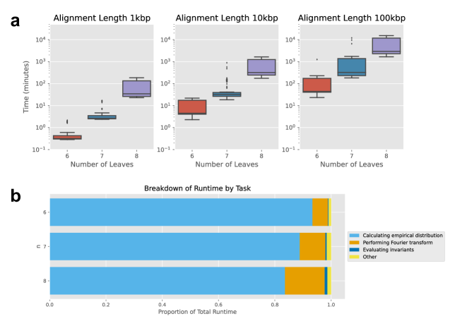
Figure 3. a. Box plots displaying the run times for $n=6,7,$ and $8$, split by alignment length.b. Breakdown of run time by task over 100 alignments of length 1kbp for each $n=6,7,8$.

Appendix A The Cohen-Macaulay Property

In this section, we use the fact that $G_{n}$ is a Gröbner basis of $\langle G_{n}\rangle$ to give an alternate proof of the dimension of $\langle G_{n}\rangle$ with Stanley-Reisner theory. We then show that the ideal $\langle G_{n}\rangle$ is Cohen-Macualay by showing that the associated simplicial complex is shellable.

Recall that the monomial ideal $\mathrm{in}_{<}(\langle G_{n}\rangle)$ is generated by the monomials $x_{i,\ell}x_{j,k}$ where $1<i<j<k<\ell<n$ and $x_{1,j_{1}}x_{i_{2},j_{2}}x_{j_{3},i_{3}}$ where $1<i_{2}<j_{1}<j_{2}<j_{3}<i_{3}\leq n$.

Now consider the simplicial complex $\Delta_{n}$ with ground set $S_{n}=\{(i,j)\leavevmode\nobreak\ |\leavevmode\nobreak\ 1\leq i<j\leq n\}$ whose minimal non-faces are given by indices appearing in each of the monomials appearing above. Given a face $F$ of $\Delta_{n}$, we define $x_{F}$ to be the product of all $x_{i,j}$ such that $(i,j)\in F$. In order to describe the facets of $\Delta_{n}$, we need to recall the definition of a Dyck path.

Definition A.1.

A Dyck path $\mathcal{D}$ from $(2,3)$ to $(n-1,n)$ is a lattice path $P=(p_{1},\dotsc,p_{2n-5})$ where

• $p_{1}=(2,3)$,

• $p_{2n-5}=(n-1,n)$,

• $p_{i+1}-p_{i}=(1,0)$ or $(0,1)$ for all $1\leq i<2n-5$, and

• if $p_{i}=(a,b)$, then $a<b$.

We say a Dyck path $\mathcal{D}$ dominates another Dyck path $\mathcal{D}^{\prime}$ if $\mathcal{D}^{\prime}$ lies between the Dyck path $\mathcal{D}$ and the line $y=x+1$.

Remark A.2.

We can partially order the set of Dyck paths via $\mathcal{D}<\mathcal{D}^{\prime}$ if $\mathcal{D}$ dominates $\mathcal{D}^{\prime}$. This poset on the set of Dyck paths from $(2,3)$ to $(n-1,n)$ has meets and joins.

For a face $F\prec\Delta_{n}$ we break it up into two pieces $F=F_{1}\cup F_{2}$ where $F_{1}=\{(1,j)\leavevmode\nobreak\ |\leavevmode\nobreak\ (1,j)\in F\}$ and $F_{2}=F\setminus F_{1}$.

Lemma A.3.

Suppose $F=F_{1}\cup F_{2}$ is a face of $\Delta_{n}$ with $F_{1}$ and $F_{2}$ as above. Then $F_{2}\subseteq\mathcal{D}$ for some Dyck path $\mathcal{D}$. If $F$ is a facet, then $(1,2),(1,n-2),(1,n-1),(1,n)\in F$.

Proof.

For the first statement, this is exactly what it means for $x_{i,\ell}x_{j,k}$ not to divide $x_{F}$ for all $1<i<j<k<\ell<n$. The second statement follows since none of these indices appear in any leading term. ∎

In the following proposition, we stratify the facets of $\Delta_{n}$ in terms of $F_{1}$ and $F_{2}$.

Proposition A.4.

$\Delta_{n}$ is a pure simplicial complex of dimension $2n-2$. If $F\prec\Delta_{n}$ is a facet, then for each $3\leq j\leq n-3$, one of the following has to occur.

1. If $x_{1,j}\leavevmode\nobreak\ |\leavevmode\nobreak\ x_{F}$, then we must be in exactly one of the following situations.

   1. $x_{F_{2}}$ is not divisible by any term in the following rectangular region of $\Omega^{n}$.

      $$\begin{pmatrix}x_{2,j+1}&\ldots&x_{2,n-2}\\ \vdots&\ddots&\vdots\\ x_{j-1,j+1}&\ldots&x_{j-1,n-2}\end{pmatrix}$$

      Moreover, $x_{F_{2}}$ divides a Dyck path monomial $x_{\mathcal{D}}$. Let $x_{i,j}$ be the last point on $\mathcal{D}$ before it enters this region, and let $x_{k,\ell}$ be the first point that exits this region on $\mathcal{D}$. Then, there are two possibilities for the Dyck path.

      1. Either $(i,j)=(j-1,j)$ and $(k,\ell)=(j,j+1)$ for some $j+1\leq\ell\leq n-2$, and the Dyck path contains $(j-1,j+1)$, or

      2. $(k,\ell)=(i,n-1)$, and the Dyck path is a horizontal line across this region. In this case, we must have $x_{1,j^{\prime}}\leavevmode\nobreak\ |\leavevmode\nobreak\ x_{F}$ for all $j^{\prime}\geq j$.

   2. $x_{F_{2}}$ is not divisible by any term in the following upper triangular region of $\Omega^{n}$.

      $$\begin{pmatrix}0&x_{j+2,j+3}&\ldots&\ldots&x_{j+2,n}\\ &0&\ddots&\ddots&\vdots\\ &&\ddots&\ddots&\vdots\\ &&&0&x_{n-1,n}\\ &&&&0\end{pmatrix}$$

      Moreover, $x_{F_{2}}$ divides a Dyck path monomial $x_{\mathcal{D}}$ where $x_{j+1,n}$ is a factor of $x_{\mathcal{D}}$. Also, in this case, we must have that $x_{1,j^{\prime}}\leavevmode\nobreak\ |\leavevmode\nobreak\ x_{F_{1}}$ for all $j^{\prime}\geq j$.

2. If $x_{1,j}$ does not divide $x_{F}$, then $j$ places no further restrictions on the Dyck path from $x_{2,3}$ to $x_{n-1,n}$.

Proof.

Let $F$ be a facet. As a first case, consider when there is no $x_{1,j}\leavevmode\nobreak\ |\leavevmode\nobreak\ x_{F}$ for $3\leq j\leq n-3$. Then $F$ is of the form $\{(1,2),(1,n-2),(1,n-1),(1,n)\}\cup\mathcal{D}$ where $\mathcal{D}$ is any Dyck path from $(2,3)$ to $(n-1,n)$. Indeed, first note that $F$ is in $\Delta_{n}$ since $x_{F}$ is not divisible by any leading term of the Gröbner basis. Second, note that if $F^{\prime}$ strictly contains $F$, then there is some $(i,j)\in F^{\prime}\setminus F$. Note that if $i=1$, there would be a degree $3$ initial term which divides $x_{F^{\prime}}$. On the other hand, if $i>1$, there would be a degree 2 initial term dividing $x_{F^{\prime}}$. It follows that if $F^{\prime}\supset F$, then $F^{\prime}\notin\Delta_{n}$; hence, $F$ is a facet of $\Delta_{n}$. Then the cardinality of $F$ is $4+(2n-5)=2n-1$, so $\dim(F)=2n-2$.

Now, suppose that $x_{1,j}\leavevmode\nobreak\ |\leavevmode\nobreak\ x_{F}$. In order for $F$ to be a face of $\Delta_{n}$, $x_{F}$ cannot be divisible by any term of the form

$$x_{1,j}x_{i_{2},j_{2}}x_{j_{3},i_{3}}\text{ where }1<i_{2}<j<j_{2}<j_{3}<i_{3}\leq n.$$

Since $x_{1,j}\leavevmode\nobreak\ |\leavevmode\nobreak\ x_{F}$, we must either omit all such $x_{i_{2},j_{2}}$ or all such $x_{j_{3},i_{3}}$. Since $F$ is a facet, we only want to omit one such collection. Suppose we are in the first case and we want to omit all $x_{i_{2},j_{2}}$. The indices of interest here are

$$U_{j}=\{(i_{2},j_{2})\leavevmode\nobreak\ |\leavevmode\nobreak\ 2\leq i_{2}\leq j-1\text{ and }j+1\leq j_{2}\leq n-2\}.$$

This is exactly the rectangular region in (1a) from the statement of the proposition. Now $F_{2}$ is contained in possibly many Dyck paths $\mathcal{D}$, we will associate $F_{2}$ with the “most efficient” such Dyck path. Suppose $(i,j)$ is the last point in $F_{2}$ before the path enters $U_{j}$, and let $(k,\ell)$ be the first point in $F_{2}$ after it leaves the region $U_{j}$.

First, we will suppose that $\ell=j+1$, i.e., the Dyck path passes through the bottom of the rectangular region $U_{j}$ in the matrix. Since we are removing all the points that are contained in the $U_{j}$, we could append all points of the form $(i^{\prime},j)$ and $(j,j^{\prime})$ where $i\leq i^{\prime}\leq j-1$ and $j+1\leq j^{\prime}\leq\ell$ to $F_{2}$ and still have a face of $\Delta_{n}$. However, since $F_{2}$ is a facet, this cannot be possible and $(i,j)=(j-1,j)$, $(k,\ell)=(j,j+1)$ and $\mathcal{D}$ must be as claimed. Note that this does not change the cardinality of $F$ from $2n-1$ since we included $(1,j)$ and removed $(j-1,j+1)$.

Secondly, suppose that $\ell=n-1$, so the first point that leaves $U_{j}$ is in the $(n-1)^{\text{th}}$ column of $\Omega^{n}$. We claim that $i=k$. Indeed, if this were not the case, then we could append all points $(k^{\prime},n-1)$ to $F_{2}$ where $i\leq k^{\prime}\leq n-1$ and still lie in $\Delta_{n}$. As $F$ is a facet, this is not possible, and $(k,\ell)=(i,n-1)$, and the Dyck path associated to $F$ is as claimed. Moreover, in this case, we evidently do not have any points in $F_{2}$ which are contained in $U_{j^{\prime}}$ for any $j\leq j^{\prime}\leq n-3$; therefore, in order for $F$ to be a facet, $(1,j^{\prime})$ must be in $F$ for all $j^{\prime}\geq j$. In this case, as well, the cardinality of $F$ remains unchanged since we removed $n-j-3$ elements from the Dyck path but added in $n-j-3$ elements from the first row.

This covers all cases when $F$ contains $(1,j)$ but does not contain any elements of the form $(i_{2},j_{2})$ where $1<i_{2}<j<j_{2}<j_{3}<i_{3}\leq n$. It remains to consider the case when $F$ contains $(1,j)$ but does not contain any elements of the form $(j_{3},i_{3})$. In this final case, we need to omit all points in the Dyck path from the following set:

$$L_{j}=\{(j_{3},i_{3})\leavevmode\nobreak\ |\leavevmode\nobreak\ j+2\leq j_{3}<i_{3}\leq n\}.$$

Note that these are the indices of the upper triangular region of the matrix from (1b) in the statement of the theorem.

Suppose $(j+1,\ell)$ is the last point in $F_{2}$ before the Dyck path enters $L_{j}$. We claim that $\ell=n$. Indeed, if it were not, then we could append $(j+1,\ell^{\prime})$ to $F_{2}$ for all $\ell^{\prime}\geq\ell$ and still be a face $\Delta_{n}$, but as $F$ is a facet, this cannot be possible, so $\ell=n$. Moreover, since we have no elements from $L_{j}$ and $L_{j^{\prime}}\subseteq L_{j}$ for all $j^{\prime}\geq j$, we are free to add $(1,j^{\prime})$ to $F_{1}$ for all such $j^{\prime}$, and since $F$ is a facet, $F$ must have already contained these elements. Finally, note that we have removed $n-j-3$ elements from the Dyck path $\mathcal{D}$ to get $F_{2}$; however, we have added in $n-j-3$ elements of the form $(1,j^{\prime})$ to $F_{1}$, so the cardinality of $F$ remains constant at $2n-1$.

We have now enumerated all facets of $\Delta_{n}$. Each facet has cardinality $2n-1$, so $\Delta_{n}$ is pure of dimension $2n-2$. ∎

Corollary A.5.

The dimension of $\mathcal{V}(\langle G_{n}\rangle)$ is $2n-1$.

Proof.

The dimension of a Stanley-Reisner ring $\mathbb{K}[\Delta]$ for a simplicial comlex $\Delta$ is $1+\dim(\Delta)$. The dimension of the variety in question is the Krull dimension of $X_{n}/\langle G_{n}\rangle$ which is equal to the Krull dimension of $X_{n}/\mathrm{in}_{>}(\langle G_{n}\rangle)$. It then follows by Proposition A.4 that the dimension of $\mathcal{V}(\langle G_{n}\rangle)=2n-1$. ∎

We end this section by showing that $\Delta_{n}$, in addition to being pure, is shellable. In particular, this implies that $\mathcal{V}(\langle G_{n}\rangle)$ is Cohen-Macaulay. To this end, we make another definition and then define a partial ordering on the facets of $\Delta_{n}$.

Definition A.6.

Let $F$ be a facet of $\Delta_{n}$. We assign a desicion function

$$\mathbf{d}_{F}:\{j\leavevmode\nobreak\ |\leavevmode\nobreak\ 3\leq j\leq n-3\}\to\{N,U,L\}$$

as follows.

1. If $(1,j)$ is not in $F$, then $\mathbf{d}_{F}(j)=N$.

2. If $(1,j)\in F$, $F_{2}\cap U_{j}=\emptyset$, and $F_{2}\cap L_{j}\neq\emptyset$, then $\mathbf{d}_{F}(j)=U$.

3. If $(1,j)\in F$, $F_{2}\cap U_{j}\neq\emptyset$, and $F_{2}\cap L_{j}=\emptyset$, then $\mathbf{d}_{F}(j)=L$.

Remark A.7.

Note the the decision function $\mathbf{d}_{F}$ tells us on what regions of the matrix $\Omega^{n}$ that $F_{2}$ is supported.

If $F,F^{\prime}\in\Delta$ are facets and $\mathcal{D},\mathcal{D}^{\prime}$ are the Dyck paths associated to $F$ and $F^{\prime}$ as in Proposition A.4, then $F\preceq F^{\prime}$ if and only if the following conditions hold.

1. $F_{1}\subseteq F_{1}^{\prime}$

2. $\mathcal{D}$ dominates $\mathcal{D}^{\prime}$

3. $\mathbf{d}_{F}(j)=\mathbf{d}_{F^{\prime}}(j)$ for all $3\leq j\leq n-3$ such that $(1,j)\in F_{1}$

Lemma A.8.

Suppose $F^{\prime}$ covers $F$. One of the following holds

1. $F_{1}=F_{1}^{\prime}$, then $F_{2}$ and $F_{2}^{\prime}$ differ in exactly one position, i.e., the cardinality of their symmetric difference is 2.

2. They are supported on the same Dyck path, $F_{1}\subseteq F_{1}^{\prime}$ where $|F_{1}^{\prime}|=|F_{1}|+1$ and $F_{2}^{\prime}\subseteq F_{2}$ with $|F_{2}^{\prime}|+1=|F_{2}|$.

In either case, $F^{\prime}\cap F$ is a facet of $\partial F^{\prime}$.

Proof.

First, suppose that $F^{\prime}$ covers $F$ and $F_{1}=F_{1}^{\prime}$. We know that $\mathcal{D}$ dominates $\mathcal{D}^{\prime}$. Since $\mathbf{d}_{F}(j)=\mathbf{d}_{F^{\prime}}(j)$ for all $3\leq j\leq n-3$ such that $(1,j)\in F_{1}$, we know that $F_{2}$ and $F_{2}^{\prime}$ are supported on the same regions of the matrix $\Omega^{n}$. If $F_{2}$ and $F_{2}^{\prime}$ differ in more than one position, then there are at least two corners of $\mathcal{D}^{\prime}\cap F_{2}^{\prime}$ which could be “flipped”, i.e. there are two elements of the form $(i,j)$ which could be replaced by $(i-1,j+1)$ in $F_{2}^{\prime}$ and the resulting Dyck path would still be dominated by $\mathcal{D}$. Flipping just one such corner gives an intermediate facet between $F^{\prime}$ and $F$. Therefore, if $F^{\prime}$ covers $F$ and $F_{1}=F_{1}^{\prime}$, then $F_{2}$ and $F_{2}^{\prime}$ differ in exactly one position and $F_{2}\triangle F_{2}^{\prime}=\{(i,j),(i-1,j+1)\}$ for some $(i,j)$. In this case, $F^{\prime}\cap F=F^{\prime}\setminus\{(i,j)\}$ which is a facet of $\partial F^{\prime}$.

Now, suppose $F^{\prime}$ covers $F$ and $F_{1}\subset F_{1}^{\prime}$. In this case, $F_{2}$ must contain $F_{2}^{\prime}$. If this were not the case, then as $\mathcal{D}$ dominates $\mathcal{D}^{\prime}$ and since $\mathbf{d}_{F}(j)=\mathbf{d}_{F^{\prime}}(j)$ for all $3\leq j\leq n-3$ such that $(1,j)\in F_{1}$, there would be an intermediate $F^{\prime\prime}$ where we take $F_{1}^{\prime\prime}$ to be $F_{1}$ and $F_{2}^{\prime\prime}$ to be $\mathcal{D}$ supported on the same regions as $\mathcal{D}^{\prime}$. As we have established that $F_{2}\supset F_{2}^{\prime}$, we must have that $F_{1}^{\prime}=F_{1}\cup\{(1,j)\}$ for some $j$ as there can be no intermediate subsets between $F_{1}$ and $F_{1}^{\prime}$. Finally, note that $F^{\prime}\cap F=F^{\prime}\setminus\{(1,j)\}$ which is a facet of $\partial F^{\prime}$. ∎

Lemma A.9.

Let $<$ be any linear extension of the partial order $\prec$. Suppose $F$ and $F^{\prime}$ are facets with $F<F^{\prime}$, and let $G_{1},\dotsc,G_{k}$ be all facets that are covered by $F^{\prime}$. Then $F\cap F^{\prime}\subset\left(\bigcup_{i=1}^{k}G_{i}\right)\cap F^{\prime}$.

Proof.

We will construct a facet $G$ with $G\prec F^{\prime}$ so that $F\cap F^{\prime}\subset G\cap F^{\prime}$. Let $\mathcal{D}^{\prime}$ and $\mathcal{D}$ be the Dyck paths associated to the facets $F^{\prime}$ and $F$, respectively. Let $\mathcal{D}_{G}$ be the join of $\mathcal{D}$ and $\mathcal{D}^{\prime}$, i.e., $\mathcal{D}_{G}$ dominates both $\mathcal{D}$ and $\mathcal{D}^{\prime}$ and is dominated by all other Dyck paths with this property. Let $G_{1}$ be the intersection $F_{1}\cap F_{1}^{\prime}$, and define a decision function $\mathbf{d}$ to be as follows.

$$\mathbf{d}(j)=\begin{cases}\mathbf{d}_{F^{\prime}}(j)&\text{if }j\in G_{1}\\ N&\text{otherwise}\end{cases}$$

Let

$$G_{2}=\mathcal{D}_{G}\setminus\left(\left(\bigcup_{j\leavevmode\nobreak\ :\leavevmode\nobreak\ \mathbf{d}(j)=L}U_{j}\right)\cup\left(\bigcup_{j\leavevmode\nobreak\ :\leavevmode\nobreak\ \mathbf{d}(j)=U}L_{j}\right)\right).$$

Finally, let $G=G_{1}\cup G_{2}$. By construction, we have that $G\prec F^{\prime}$ and $F\cap F^{\prime}\subset F\cap G$. Thus, we have reduced to the case when $F\prec F^{\prime}$.

Now that we have reduced to the case when $F\prec F^{\prime}$, consider a chain

$$F=F^{(0)}\prec\dotsc\prec F^{(k)}=F^{\prime}$$

in the poset where $F^{(i+1)}$ covers $F^{(i)}$ for all $i$. We may choose this chain so that the first say $\ell$ facets are adding elements to $F^{(i)}_{1}$ and removing an element from $F^{(i)}_{2}$; then past $\ell$, the elements in $F^{(i)}_{1}$ remain constant and then each subsequent facet in the chain is obtained by “flipping a corner” of the previous Dyck path. Going through this process, we see that $F^{(i-1)}\cap F^{\prime}$ is a subset of $F^{(i)}\cap F^{\prime}$ for all $1\leq i\leq k$. In particular, $F\cap F^{\prime}$ is a subset of $F^{(k-1)}\cap F^{\prime}$ which lies in the boundary of $\partial F^{\prime}$. ∎

Proposition A.10.

Let $<$ be any linear extension of the partial order $\prec$. Then $<$ is a shelling order for $\Delta_{n}$.

Proof.

Let $<$ be such a linear extension, so we have $F^{(1)}<F^{(2)}<\dots$ for the facets of $\Delta_{n}$. We must show for every $k>1$ that

$$B_{k}=\left(\bigcup_{i=1}^{k-1}F^{(i)}\right)\cap F^{(k)}$$

is a non-empty union of facets of $\partial F^{(k)}$. This follows from Lemma A.8 and Lemma A.9. ∎

Corollary A.11.

The quotient ring $X_{n}/\langle G_{n}\rangle$ is Cohen-Macualay.

References

• [1] Elizabeth S Allman, Hector Baños, and John A Rhodes. Nanuq: a method for inferring species networks from gene trees under the coalescent model. Algorithms for Molecular Biology, 14:1–25, 2019.
• [2] Elizabeth S. Allman, Colby Long, and John A. Rhodes. Species tree inference from genomic sequences using the log-det distance. SIAM Journal on Applied Algebra and Geometry, 3(1):107–127, 2019.
• [3] Elizabeth S. Allman and John A. Rhodes. Phylogenetic invariants for the general markov model of sequence mutation. Mathematical Biosciences, 186(2):113–144, 2003.
• [4] Elizabeth S. Allman and John A. Rhodes. Phylogenetic ideals and varieties for the general markov model. Advances in Applied Mathematics, 40(2):127–148, 2008.
• [5] Hector Baños. Identifying species network features from gene tree quartets under the coalescent model. Bulletin of mathematical biology, 81:494–534, 2019.
• [6] Travis Barton, Elizabeth Gross, Colby Long, and Joseph Rusinko. Statistical learning with phylogenetic network invariants. arXiv 2211.11919, 2022.
• [7] Marta Casanellas and Jesús Fernández-Sánchez. Performance of a new invariants method on homogeneous and nonhomogeneous quartet trees. Molecular Biology and Evolution, 24(1):288–293, 2007.
• [8] Marta Casanellas and Jesús Fernández-Sánchez. Rank conditions on phylogenetic networks. In Extended Abstracts GEOMVAP 2019: Geometry, Topology, Algebra, and Applications; Women in Geometry and Topology, pages 65–69. Springer, 2021.
• [9] David A. Cox, John Little, and Donal O’Shea. Ideals, Varieties, and Algorithms: An Introduction to Computational Algebraic Geometry and Commutative Algebra. Springer Publishing Company, Incorporated, 3rd edition, 2010.
• [10] Joseph Cummings, Benjamin Hollering, and Christopher Manon. Invariants for level-1 phylogenetic networks under the Cavendar-Farris-Neyman model. Advances in Applied Mathematics, 153:102633, 2024.
• [11] Steven N. Evans and T. P. Speed. Invariants of some probability models used in phylogenetic inference. Ann. Statist., 21(1):355–377, 1993.
• [12] Elisa Gorla. Mixed ladder determinantal varieties from two-sided ladders. J. Pure Appl. Algebra, 211(2):433–444, 2007.
• [13] Daniel R. Grayson and Michael E. Stillman. Macaulay2, Version 1.20, 2022. http://www.math.uiuc.edu/Macaulay2/.
• [14] Elizabeth Gross, Robert Krone, and Samuel Martin. Dimensions of level-1 group-based phylogenetic networks. arXiv:2307.15166, 2023.
• [15] Elizabeth Gross and Colby Long. Distinguishing phylogenetic networks. SIAM Journal on Applied Algebra and Geometry, 2(1):72–93, 2018.
• [16] Elizabeth Gross, Colby Long, and Joseph Rusinko. Phylogenetic networks. A Project-Based Guide to Undergraduate Research in Mathematics: Starting and Sustaining Accessible Undergraduate Research, pages 29–61, 2020.
• [17] Elizabeth Gross, Leo van Iersel, Remie Janssen, Mark Jones, Colby Long, and Yukihiro Murakami. Distinguishing level-1 phylogenetic networks on the basis of data generated by markov processes. Journal of Mathematical Biology, 83:1–24, 2021.
• [18] Michael D Hendy and David Penny. Complete families of linear invariants for some stochastic models of sequence evolution, with and without the molecular clock assumption. Journal of Computational Biology, 3(1):19–31, 1996.
• [19] Benjamin Hollering and Seth Sullivant. Identifiability in phylogenetics using algebraic matroids. Journal of Symbolic Computation, 104:142–158, 2021.
• [20] Colby Long. Initial ideals of Pfaffian ideals. Journal of Commutative Algebra, 12(1):91 – 105, 2020.
• [21] Samuel Martin, Vincent Moulton, and Richard M. Leggett. Algebraic invariants for inferring 4-leaf semi-directed phylogenetic networks. bioRxiv 2023.09.11.557152, 2023.
• [22] The mpmath development team. mpmath: a Python library for arbitrary-precision floating-point arithmetic, 2023. http://mpmath.org/.
• [23] MATHREPO Mathematical Data and Software. https://mathrepo.mis.mpg.de/PfaffianPhylogeneticNetworks, 2023. [Online; accessed 17 October 2023].
• [24] The scikit-bio development team. scikit-bio: A Bioinformatics Library for Data Scientists, Students, and Developers, 2020. http://scikit-bio.org/.
• [25] Mike Steel. Phylogeny: discrete and random processes in evolution. SIAM, 2016.
• [26] Bernd Sturmfels. Solving systems of polynomial equations, volume 97 of CBMS Regional Conference Series in Mathematics. Conference Board of the Mathematical Sciences, Washington, DC; by the American Mathematical Society, Providence, RI, 2002.
• [27] Bernd Sturmfels and Seth Sullivant. Toric ideals of phylogenetic invariants. Journal of Computational Biology, 12(2):204–228, 2005.
• [28] Seth Sullivant. Toric fiber products. J. Algebra, 316(2):560–577, 2007.
• [29] Seth Sullivant. Algebraic statistics, volume 194 of Graduate Studies in Mathematics. American Mathematical Society, Providence, RI, 2018.
• [30] Zhaoxing Wu and Claudia Solis-Lemus. Ultrafast learning of 4-node hybridization cycles in phylogenetic networks using algebraic invariants. arXiv preprint arXiv:2211.16647, 2022.