Simplifying QCD event generation with chirality flow, reference vectors and spin directions

Abstract

The chirality-flow formalism, combined with good choices of gauge reference vectors, simplifies tree-level calculations to the extent that it is often possible to write down amplitudes corresponding to Feynman diagrams immediately. It has also proven to give a very sizable speedup in a proof of concept implementation of massless tree-level QED in MadGraph5_aMC@NLO. In the present paper we extend this analysis to QCD, including massive quarks. We define helicity-dependent versions of the gluon vertices, derive constraints on the spinor structure of propagating gluons, and explore the Schouten identity to simplify the four-gluon vertex further. For massive quarks, the chirality-flow formalism sheds light on how to exploit the freedom to measure spin along any direction to shorten the calculations. Overall, this results in a clear speedup for treating the Lorentz structure at high multiplicities.

1 Introduction

Tools for simulating events at the LHC and other collider experiments tend to employ Feynman diagram methods to compute helicity amplitudes, i.e., amplitudes with assigned helicities Gleisberg:2008fv ; Alwall:2014hca ; Sjostrand:2014zea ; Bellm:2015jjp ; Sherpa:2019gpd . Such calculations, especially for massless particles, benefit from utilizing the spinor-helicity formalism Farrar:1983wk ; Berends:1987cv ; Berends:1987me ; Berends:1988yn ; Berends:1988zn ; Berends:1989hf ; Murayama:1992gi ; Dittmaier:1993bj ; Dittmaier:1998nn ; Weinzierl:2005dd ; Gleisberg:2008fv . For treating the color structure, orthogonal bases, based on representation theory could be used Keppeler:2012ih ; Sjodahl:2015qoa ; Du:2015apa ; Alcock-Zeilinger:2022hrk , but so far, in practice typically trace or color-flow bases are employed tHooft:1973alw ; Kanaki:2000ms ; Maltoni:2002mq ; Weinzierl:2005dd ; Kilian:2012pz ; Sjodahl:2012nk ; Reuschle:2013qna ; Sjodahl:2014opa .

In a few recent papers Lifson:2020pai ; Alnefjord:2020xqr ; Lifson:2023wow the Lorentz structure analogue of the color-flow picture was developed, by also “flowing” the spin and momentum structure of amplitudes. Similar to the color-flow Feynman rules, a complete set of chirality-flow Feynman rules were developed for the standard model in Alnefjord:2020xqr ; Lifson:2023wow . These chirality-flow rules, where the Fierz identity has been built in (like the color Fierz identity for color flow), is easily seen to significantly simplify tree-level calculations by hand Lifson:2020pai ; Alnefjord:2020xqr . Recently it has also proven to give a sizable speedgain for a numerical tree-level massless QED implementation within MadGraph5_aMC@NLO Alwall:2014hca , where the computation time is reduced by more than a factor 10 for $e^{+}e^{-}$ going to seven photons Lifson:2022ijv .

This improvement is in part attributed to the simpler Lorentz structure for the (massless) QED vertex, and in part due the choice of gauge reference vector for external photons. While polarization vectors typically are taken to be orthogonal to the momentum $p$ and a four-vector with the sign of the spatial part swapped, one may perfectly well describe polarization vectors as being orthogonal to some other (lightlike) reference momentum $r$, aside from $p$ Xu:1986xb ; Mangano:1987xk .

In this paper we address QCD and explore the simplifications and speedgains achieved by clever choices of reference and spin vectors, combined with simplified versions of the chiral three- and four-gluon vertices. In particular, this makes it possible to retain information about the spinor structure of internal gluons. In this context we also exploit the Schouten identity.

Although most strongly interacting particles effectively are massless, the top quark requires a mass. We therefore address the complications brought about by adding fermion masses; while massless fermions naturally lend themselves to a description in terms of single Weyl spinors, massive fermions necessarily come with both a left- and a right-chiral component, which unavoidably complicates the calculations. However, also in this case, a clever choice of the reference vector — which now has acquired a physical interpretation, being related to the direction in which spin is measured — can be explored to reduce the computational complexity. Effectively, we thereby take advantage of the freedom to measure spin in any direction in order to simplify calculations.

To set the stage of our implementation, we introduce the chirality-flow formalism in the following section. After that, we describe the context within which the chirality-flow version of QCD is implemented in section 3, where we outline the HELAS algorithm Murayama:1992gi and its implementation within MadGraph5_aMC@NLO. The algebraic simplifications from gauge dependent Feynman rules are explored in section 4, and the resulting speedgains in section 5. Finally, we conclude and discuss future perspectives in section 6.

2 Chirality flow

By noting that the Lie algebra $\mathfrak{so}(1,3)$ of the restricted Lorentz group SO(1,3) can be decomposed into two copies of the SL(2,$\mathbb{C}$) Lie algebra $\mathfrak{sl}(2,\mathbb{C})$, the spinor-helicity (DeCausmaecker:1981jtq, ; Berends:1981rb, ; Berends:1981uq, ; DeCausmaecker:1981wzb, ; Berends:1983ez, ; Kleiss:1984dp, ; Berends:1984gf, ; Gunion:1985bp, ; Gunion:1985vca, ; Kleiss:1986qc, ; Hagiwara:1985yu, ; Kleiss:1985yh, ; Kleiss:1986ct, ; Xu:1986xb, ; Gastmans:1987qz, ; Schwinn:2005pi, ) and Weyl-van-der-Waerden (Farrar:1983wk, ; Berends:1987me, ; Berends:1987cv, ; Berends:1988yn, ; Berends:1988zn, ; Berends:1989hf, ; Dittmaier:1993bj, ; Dittmaier:1998nn, ; Weinzierl:2005dd, ) formalisms split Minkowski four-space into two two-component spinor spaces. In chirality flow, we further incorporate the Fierz identity for the Pauli matrices,

$$\sigma^{\mu,\dot{\alpha}\beta}\bar{\sigma}_{\mu,\alpha\dot{\beta}}=2\delta^{\dot{\alpha}}_{\ \dot{\beta}}\delta^{\ \beta}_{\alpha},$$ (2.0.1)

directly into our Feynman rules, analogous to how gluons are split into color and anti-color lines in QCD tHooft:1973alw ; Kanaki:2000ms ; Maltoni:2002mq . This gives rise to a flow-description of chiral representations of Feynman rules and diagrams, dubbed the chirality-flow formalism (Lifson:2020pai, ; Alnefjord:2020xqr, ; Lifson:2023wow, ). Below we go through the essence of chirality-flow Feynman rules. Our conventions are extensively detailed in ref. (Lifson:2020pai, ).

2.1 A graphical representation of fermions and gauge bosons

The fundamental building blocks for calculations in the spinor helicity formalism in general are the left- and right-chiral Weyl spinors, which we graphically represent as

$${\color[rgb]{1,0,0}\langle}i{\color[rgb]{1,0,0}|} =\raisebox{-0.3pt}{\includegraphics[scale={0.4}]{Jaxodraw/MS/ExtSpinorSolidiCol}},\qquad{\color[rgb]{0,0,1}[}i{\color[rgb]{0,0,1}|} =\raisebox{-0.3pt}{\includegraphics[scale={0.4}]{Jaxodraw/MS/ExtSpinorDottediCol}},$$

$${\color[rgb]{1,0,0}|}j{\color[rgb]{1,0,0}\rangle} =\raisebox{-0.3pt}{\includegraphics[scale={0.4}]{Jaxodraw/MS/ExtSpinorSolidjCol}},\qquad{\color[rgb]{0,0,1}|}j{\color[rgb]{0,0,1}]} =\raisebox{-0.3pt}{\includegraphics[scale={0.4}]{Jaxodraw/MS/ExtSpinorDottedjCol}},$$ (2.1.1)

where ${\color[rgb]{1,0,0}\langle}i{\color[rgb]{1,0,0}|}={\color[rgb]{1,0,0}\langle}p_{i}{\color[rgb]{1,0,0}|}$ etc. We define the direction of chirality flow such that following the arrow direction is equivalent to reading from left to right in an equation. Thus the Lorentz invariant spinor inner products are given by

$${\color[rgb]{1,0,0}\langle}ij{\color[rgb]{1,0,0}\rangle}\equiv\epsilon^{\alpha\beta}\lambda_{i,\beta}\lambda_{j,\alpha}={\includegraphics[scale={0.4}]{Jaxodraw/MS/SpinorProdAngleijCol}}~{},\;\;\;{\color[rgb]{0,0,1}[}ij{\color[rgb]{0,0,1}]}\equiv\epsilon_{{\dot{\alpha}}{\dot{\beta}}}\tilde{\lambda}_{i}^{{\dot{\beta}}}\tilde{\lambda}_{j}^{{\dot{\alpha}}}=\raisebox{-0.2pt}{\includegraphics[scale={0.4}]{Jaxodraw/MS/SpinorProdSquareijCol}}~{},$$ (2.1.2)

with (antisymmetric) ${\color[rgb]{1,0,0}\langle}ij{\color[rgb]{1,0,0}\rangle}\sim{\color[rgb]{0,0,1}[}ij{\color[rgb]{0,0,1}]}\sim\sqrt{2p_{i}\cdot p_{j}}$, up to a phase factor.

While there is a simple relationship between massless fermions and Weyl spinors, e.g.

$$u^{+}(p)\;=\;\begin{pmatrix}0\\ \raisebox{-5.5pt}{\includegraphics[scale={0.375}]{./Jaxodraw/MS/ExtSpinorAntiSolid_pCol}}\end{pmatrix}\rightarrow\raisebox{-5.5pt}{\includegraphics[scale={0.375}]{./Jaxodraw/MS/ExtSpinorAntiSolid_pCol}},\quad p^{2}=0,$$ (2.1.3)

we also need to describe vector bosons and massive fermions. In order to treat massive momenta $p$, we decompose them in terms of two lightlike momenta $p^{\flat}$ and $q$ by

$$p^{\mu}=p^{\flat,\mu}+\alpha q^{\mu}~{},\qquad(p^{\flat})^{2}=q^{2}=0,\qquad p^{2}=m^{2}~{},\qquad\alpha=\frac{m^{2}}{2p^{\flat}\cdot q}=\frac{m^{2}}{2p\cdot q}~{}.$$ (2.1.4)

Note that eq. (2.1.4) does not determine the decomposition $p=p^{\flat}+\alpha q$ uniquely. This is related to the freedom to measure spin along any axis (Kleiss:1985yh, ; Dittmaier:1998nn, ),

$$s^{\mu}=\frac{1}{m}\left(p^{\flat,\mu}-\alpha q^{\mu}\right)=\frac{1}{m}\left(p^{\mu}-2\alpha q^{\mu}\right).$$ (2.1.5)

Measuring spin along the direction of motion (corresponding to $q=\frac{1}{2}(p_{0}-|\vec{p}|)(1,-\frac{\vec{p}}{|\vec{p}|})$, $\alpha=1$, $s=\frac{1}{m}(|\vec{p}|,p^{0}\frac{\vec{p}}{|\vec{p}|})$, cf. Alnefjord:2020xqr ) reproduces the helicity basis, but we will instead keep the spin direction arbitrary here, such that we can use it to reduce the complexity of the computations, a topic we discuss further in section 4.5. With this decomposition, e.g. an incoming fermion with positive spin is given by

$$u^{+}(p)=\begin{pmatrix}\frac{m}{{\color[rgb]{0,0,1}[}p^{\flat}q{\color[rgb]{0,0,1}]}}\raisebox{-0.2pt}{\includegraphics[scale={0.40}]{Jaxodraw/MS/ExtSpinorAntiDotted_qCol}}\\ \phantom{\frac{m}{{\color[rgb]{0,0,1}[}p^{\flat}q{\color[rgb]{0,0,1}]}}}\raisebox{-0.2pt}{\includegraphics[scale={0.40}]{Jaxodraw/MS/ExtSpinorAntiSolid_pflatCol}}\end{pmatrix}\;,$$ (2.1.6)

which reduces to a right-chiral Weyl spinor in the massless limit $m\rightarrow 0$, $p^{\flat}\rightarrow p$. Spinors for the other external fermions are given in appendix A.

Vector bosons necessitate both a left- and a right-chiral spinor, and can be represented by Berends:1981rb ; DeCausmaecker:1981jtq ; Mangano:1987xk ; Gunion:1985bp ; Gunion:1985vca ; Kleiss:1986qc ; Xu:1986xb ; Gastmans:1990xh ,

$$\epsilon_{\color[rgb]{0,0,1}{L}}(p_{i},r) =\frac{{\color[rgb]{0,0,1}|}i{\color[rgb]{0,0,1}]}{\color[rgb]{1,0,0}\langle}r{\color[rgb]{1,0,0}|}}{{\color[rgb]{1,0,0}\langle}ri{\color[rgb]{1,0,0}\rangle}}=\frac{1}{{\color[rgb]{1,0,0}\langle}ri{\color[rgb]{1,0,0}\rangle}}\raisebox{-0.2pt}{\includegraphics[scale={0.35}]{Jaxodraw/MS/PhotonExtFlowPlaRevCol}}\;\;\text{or}\;\;\,\,\frac{{\color[rgb]{1,0,0}|}r{\color[rgb]{1,0,0}\rangle}{\color[rgb]{0,0,1}[}i\color[rgb]{0,0,1}{|}}{{\color[rgb]{1,0,0}\langle}ri{\color[rgb]{1,0,0}\rangle}}=\frac{1}{{\color[rgb]{1,0,0}\langle}ri{\color[rgb]{1,0,0}\rangle}}\raisebox{-0.2pt}{\includegraphics[scale={0.35}]{Jaxodraw/MS/PhotonExtFlowPlaCol}},$$

$$\epsilon_{\color[rgb]{1,0,0}{R}}(p_{i},r) =\frac{{\color[rgb]{0,0,1}|}r{\color[rgb]{0,0,1}]}{\color[rgb]{1,0,0}\langle}i{\color[rgb]{1,0,0}|}}{{\color[rgb]{0,0,1}[}ir{\color[rgb]{0,0,1}]}}=\frac{1}{{\color[rgb]{0,0,1}[}ir{\color[rgb]{0,0,1}]}}\raisebox{-0.2pt}{\includegraphics[scale={0.35}]{Jaxodraw/MS/PhotonExtFlowMiaCol}}\;\;\text{or}\;\;\,\,\frac{{\color[rgb]{1,0,0}|}i{\color[rgb]{1,0,0}\rangle}{\color[rgb]{0,0,1}[}r\color[rgb]{0,0,1}{|}}{{\color[rgb]{0,0,1}[}ir{\color[rgb]{0,0,1}]}}=\frac{1}{{\color[rgb]{0,0,1}[}ir{\color[rgb]{0,0,1}]}}\raisebox{-0.2pt}{\includegraphics[scale={0.35}]{Jaxodraw/MS/PhotonExtFlowMiaRevCol}},$$ (2.1.7)

with $\epsilon_{\color[rgb]{0,0,1}{L}}$ corresponding to an incoming left helicity state or outgoing right helicity state, and $\epsilon_{\color[rgb]{1,0,0}{R}}$ corresponding to an incoming right helicity state or outgoing left helicity state. Note that the “chirality” (L/R) of a gauge boson is given by the spinor carrying its physical momentum $p_{i}$, and that $r$ is a gauge reference momentum, with $p_{i}\cdot r\neq 0$ and $r^{2}=0$. The chirality-flow directions (arrows above) can be chosen arbitrarily, as long as the two arrows making up the polarization vector are opposing each other, and are consistent with the rest of the diagram, the details of which we leave for section 2.4. The unphysical reference vector $r$ is typically set to $r=(p^{0},-\vec{p})$ both in MadGraph5_aMC@NLO and in standard QFT literature (such as for example (Peskin:1995ev, )). We will instead use this as a freedom to significantly speed up calculations, by making diagrams vanish.

In principle these simplifications are not new to chirality flow Mangano:1987xk , but the flow picture makes it obvious how to use the simplification even far inside Feynman diagrams. To the authors’ knowledge, the freedoms of choosing gauge reference vectors as well as spin directions are unexploited in major event generators. We discuss this subject further in section 2.3, and explore the benefits in section 4.

2.2 Propagators and vertices

In the previous section, we detailed the necessary structures to describe free particles within the chirality-flow formalism. To evaluate scattering amplitudes we also need to represent propagators and vertices.

As there are two non-scalar particle types within the standard model, two types of propagators are needed. We first treat the gauge boson, which in the Feynman gauge has the structure of the Minkowski metric, translating to two opposing chirality-flow lines

$$=\quad-i\frac{g_{\mu\nu}}{p^{2}} \rightarrow -\frac{i}{p^{2}}\raisebox{-0.25pt}{\includegraphics[scale={0.45}]{Jaxodraw/PhotonPropFlowa}}\;,$$ (2.2.1)

with directions to be matched with the rest of the Feynman diagram.

The fermion propagator has a more complicated structure, with a slashed momentum in the numerator. In the flow picture, this can be represented using the momentum-dot notation introduced in (Lifson:2020pai, ),

$$\not{p}\equiv\sqrt{2}p^{\mu}\tau_{\mu}^{{\dot{\alpha}}\beta}=\raisebox{-0.25pt}{\includegraphics[scale={0.4}]{./Jaxodraw/MS/FermionMomDotaColab}},\quad\quad\bar{\not{p}}\equiv\sqrt{2}p_{\mu}\bar{\tau}^{\mu}_{\alpha{\dot{\beta}}}=\raisebox{-0.25pt}{\includegraphics[scale={0.4}]{./Jaxodraw/MS/FermionMomDotbColab}}\;,$$ (2.2.2)

where we work in the chiral (Weyl) basis and use normalized versions of the Pauli matrices, $\sqrt{2}\tau^{\mu}=\sigma^{\mu}$ and $\sqrt{2}\bar{\tau}^{\mu}=\bar{\sigma}^{\mu}$, to avoid factors of 2 in the Fierz identity.

The arrow direction aligned with the rest of the diagram must be chosen, as elaborated on in section 2.4. For future purposes, we recall that these momentum-dots can be rewritten in terms of outer products of Weyl spinors,

$$=\sum_{i}{\color[rgb]{0,0,1}|}i{\color[rgb]{0,0,1}]}{\color[rgb]{1,0,0}\langle}i{\color[rgb]{1,0,0}|} =\sum_{i}{\color[rgb]{1,0,0}|}i{\color[rgb]{1,0,0}\rangle}{\color[rgb]{0,0,1}[}i{\color[rgb]{0,0,1}|}$$ and (2.2.3)

for $p_{i}^{2}=0$ such that $p=\sum_{i}p_{i}$. The fermion propagator is then

$$=\ \frac{i}{p^{2}-m^{2}}\begin{pmatrix}m{\delta^{{\dot{\alpha}}}}_{{\dot{\beta}}}&\sqrt{2}p^{{\dot{\alpha}}\beta}\\ \sqrt{2}\bar{p}_{\alpha{\dot{\beta}}}&m{\delta_{\alpha}}^{\beta}\end{pmatrix}=\frac{i}{p^{2}-m^{2}}\begin{pmatrix}m\includegraphics[scale={0.34}]{Jaxodraw/MS/KroneckerDeltaDottedPropCol}&\includegraphics[scale={0.34}]{Jaxodraw/MS/FermionPropFlowDottedSolodAlphaBetaCol}\\ \includegraphics[scale={0.34}]{Jaxodraw/MS/FermionPropFlowSolidDottedAlphaBetaCol}&m\includegraphics[scale={0.34}]{Jaxodraw/MS/KroneckerDeltaUndottedCol}\end{pmatrix}\;.$$ (2.2.4)

Finally, external particles and propagators are combined in QCD vertices. The simplest vertex is the fermion-vector vertex, represented by just a flow,

$$\includegraphics[scale={0.45},valign={c}]{Jaxodraw/fPhotonVertexMassless}\!\!\!\!\!=\frac{ig_{s}t^{a}_{i\bar{j}}}{\sqrt{2}}\gamma^{\mu} =\frac{ig_{s}t^{a}_{i\bar{j}}}{\sqrt{2}}\begin{pmatrix}0&\sqrt{2}\tau^{\mu,{\dot{\alpha}}\beta}\\ \sqrt{2}\bar{\tau}^{\mu}_{\alpha{\dot{\beta}}}&0\end{pmatrix}$$

$$\rightarrow ig_{s}t^{a}_{i\bar{j}}\begin{pmatrix}0&\raisebox{-0.35pt}{\includegraphics[scale={0.35}]{Jaxodraw/FermionVectorVertexRab}}\\ \raisebox{-0.4pt}{\includegraphics[scale={0.35}]{./Jaxodraw/FermionVectorVertexLab}}&0\end{pmatrix}~{},$$ (2.2.5)

with $g_{s}$ being the strong coupling constant and where the $\sqrt{2}$ in the denominator comes from the normalization of our SU(3) generators $t^{a}_{i\bar{j}}$, which as our matrices $\tau$, are normalized to one, $\textrm{Tr}(t^{a}t^{b})=\delta^{ab}$, $\textrm{Tr}(\tau^{i}\tau^{j})=\delta^{ij}$.

The four-gluon vertex has a simple form in chirality flow, being represented by Kronecker deltas that can be connected in three different ways,

$$=\;\;i\left(\!\frac{g_{s}}{\sqrt{2}}\right)^{\!\!2}\!\!\;\sum\limits_{Z(2,3,4)}if^{a_{1}a_{2}b}if^{ba_{3}a_{4}}\;\Big{(}g^{\mu_{1}\mu_{3}}g^{\mu_{2}\mu_{4}}-g^{\mu_{1}\mu_{4}}g^{\mu_{2}\mu_{3}}\Big{)}\;$$

$$\rightarrow\;\;i\left(\!\frac{g_{s}}{\sqrt{2}}\right)^{\!\!2}\!\!\;\sum\limits_{Z(2,3,4)}if^{a_{1}a_{2}b}if^{ba_{3}a_{4}}\left(\includegraphics[scale={0.225},valign={c}]{Jaxodraw/MS/4GluonVertex_Kin13}-\includegraphics[scale={0.225},valign={c}]{Jaxodraw/MS/4GluonVertex_Kin14}\right)~{},$$ (2.2.6)

where $Z(2,3,4)$ denotes the set of cyclic permutations of the integers $2,3,$ and $4$, $f^{abc}$ are the SU(3) structure constants, and where arrow directions which give flows aligned with the rest of the diagram are chosen, as elaborated on in section 2.4,

Finally, we address the triple-gluon vertex, which comes with the highest complexity from the chirality-flow perspective as it involves a momentum-dot. Chirality can flow between any two of the gluons (connected with the metric), while the third gluon is contracted with a momentum-dot,

$$=\;i\frac{g_{s}}{\sqrt{2}}if^{a_{1}a_{2}a_{3}}\Big{(}g^{\mu_{1}\mu_{2}}(p_{1}-p_{2})^{\mu_{3}}+g^{\mu_{2}\mu_{3}}(p_{2}-p_{3})^{\mu_{1}}+g^{\mu_{3}\mu_{1}}(p_{3}-p_{1})^{\mu_{2}}\Big{)}$$

$$\rightarrow\;i\frac{g_{s}}{\sqrt{2}}if^{a_{1}a_{2}a_{3}}\frac{1}{\sqrt{2}}\left(\includegraphics[scale={0.325},valign={c}]{Jaxodraw/MS/3GluonVertex_HelFlow1p}\!\!\!+\includegraphics[scale={0.325},valign={c}]{Jaxodraw/MS/3GluonVertex_HelFlow2p}\!\!\!+\includegraphics[scale={0.325},valign={c}]{Jaxodraw/MS/3GluonVertex_HelFlow3p}\!\!\!\right)~{},$$ (2.2.7)

where the implicit arrows again should be chosen to give a continuous flow.

2.3 Gauge based diagram removal and chirality-flow diagram removal

In a recent paper we explored the benefits of gauge based diagram removal (Lifson:2022ijv, ), i.e, the freedom to choose reference momenta for external massless gauge bosons in such a way as to make a maximal number of Feynman diagrams vanish. There we worked with QED, and set the reference momenta $r_{R}$ of all right-chiral photons to be the physical momentum of a left-chiral lepton, and similarly for left-chiral photons with a right-chiral lepton.

As a simple example, before moving on to QCD, we consider the chiral structure of the process $e^{-}_{L}e^{+}_{R}\rightarrow n\gamma$, using the chirality-flow part of the vertex in eq. (2.2.5), the massless fermion propagator from eq. (2.2.4), and massless external fermions and bosons. The corresponding diagram can then be immediately written down as

(2.3.1)

$$\propto {{\color[rgb]{0,0,1}[p_{e^{-}}\,1_{L}]}}\times{{\color[rgb]{1,0,1}\langle 1_{R}|\bar{\not{p}}_{e^{-}-1}|2_{L}]}}\times{{\color[rgb]{0,0.88,0}\langle 2_{R}|\bar{\not{p}}_{e^{-}-1-2}|3_{L}]}}\times\ldots\times{{\color[rgb]{1,0,0}\langle n_{R}\,p_{e^{+}}\rangle}}\;.$$

In passing, we note that the chirality-flow arrows are chosen to align along the fermion line, but to oppose each other for the photons, and that we could equally well have chosen to swap all arrows since, employing eq. (2.2.3), we have an even number of spinor inner products. As there is only one fermion line, each Feynman diagram can be described by the ordering of the photons. However, by setting the reference momentum of right-chiral photons to the momentum of the left-chiral fermion (and opposite),

$$i_{L}=r_{R}=p_{e^{-}_{L}}\quad\textrm{for right-chiral and}\quad i_{R}=r_{L}=p_{e^{+}_{R}}\quad\text{for left-chiral},$$ (2.3.2)

any diagram where a right-chiral photon is contracted with the left-chiral fermion will include a factor ${\color[rgb]{0,0,1}[}p_{e^{-}_{L}}{\color[rgb]{0,0,1}|}p_{e^{-}_{L}}{\color[rgb]{0,0,1}]}=0$ and vanish, and similarly for left-chiral photons. It is therefore not possible to attach a right-chiral photon next to $e^{-}_{L}$ or a left-chiral photon next to $e^{+}_{R}$. In principle this simplification is present in the spinor-helicity formalism itself, but the chirality-flow formalism makes it completely transparent.

As we consider non-abelian gauge theories, we encounter structures with several contributing chirality flows from the gauge boson vertices. Similarly massive fermion propagators give rise to more than one chirality flow. Here the choice of reference momenta or spin axes may not remove the full Feynman diagram despite removing some of the corresponding chirality-flow diagrams. Consider e.g. the chiral structure of the Feynman diagram (now counting all momenta as outgoing)

$$\raisebox{-0.5pt}{\includegraphics[scale={0.4}]{./Jaxodraw/QCDPaper/Example}}\rightarrow\underbrace{\raisebox{-0.5pt}{\includegraphics[scale={0.4}]{./Jaxodraw/QCDPaper/ExampleRHS1}}}_{0}$$ (2.3.3)

$$+\raisebox{-0.5pt}{\includegraphics[scale={0.4}]{./Jaxodraw/QCDPaper/ExampleRHS2}}+\raisebox{-0.5pt}{\includegraphics[scale={0.4}]{./Jaxodraw/QCDPaper/ExampleRHS3}}\;,\;$$

which contributes to the process $q_{1,R}\bar{q}_{5,L}\rightarrow g_{2,R}\,g_{3,L}\,g_{4,L}$ for massless quarks. Here we note that setting the gauge reference vectors of the left-chiral gluons, to the same momentum $r_{3}=r_{4}=r_{L}$, the first chirality-flow diagram vanishes for any $r_{L}$.

Despite not having removed the total contribution from this Feynman diagram, we have reduced the complexity of the Lorentz structures, by removing some chirality-flow diagrams. Therefore, we shall refer to this simplification as gauge based chirality-flow diagram removal, rather than gauge based Feynman diagram removal.

Further, if we let $r_{3}=r_{4}=r_{L}=p_{1}$, the gluons $g_{3}$ and $g_{4}$ cannot attach to $q_{1}$, implying that all such Feynman diagrams vanish. Similarly, letting $r_{2}=r_{R}=p_{5}$ gluon 2 cannot attach to $\bar{q}_{5}$. This type of simplification is in direct analogy with the gauge based Feynman diagram removal for QED as in eq. (2.3.1). However, the simplification that arises from the contraction between external gauge bosons is new for QCD. This is elaborated upon in section 4, where gauge specific Feynman rules are introduced. Additionally, by considering sums over measurements on general spin axes, rather than helicity sums, there will at times be gauge based chirality-flow diagram removal in the fermion-vector vertex, where only one of the chiral components of a massive fermion contributes to the scattering amplitude.

2.4 Chirality-flow direction

In the previous sections, we have largely neglected the question of chirality-flow direction, simply stating that it has to be made consistent. With the examples in eq. (2.3.1) and eq. (2.3.3) at hand, we are now in a good position to comment on this. To this end, we remind the reader that momentum-dots can be written as sums of massless spinor outer products (cf. eq. (2.2.3)).

Each single chirality-flow line maps to a spinor inner product, and considering massless fermions, we note that the momentum-dot in the fermion propagator ensures that every massless fermion line will have an even number of chirality-flow lines. Additionally, all vector bosons have two chirality-flow lines with opposing flow direction. In massless QCD and QED, there is thus always an even number of flow lines, making it impossible to flip an odd number of spinor inner products as long as flow continuity and the opposing arrow convention for gauge bosons are respected. By the antisymmetry of the inner product, all consistent choices of flow directions then give the same amplitude. As an example, we may choose the arrow assignment

(2.4.1)

for the second term in eq. (2.3.3).

The massive fermion propagator, however, gives rise to terms with an odd number of flows. It is then necessary to keep track of the relative sign of the mass terms and the momentum terms.

3 Flowing HELAS

MadGraph5_aMC@NLO evaluates helicity amplitudes using ALOHA-generated deAquino:2011ub code based on a recursive algorithm as for HELAS (Murayama:1992gi, ). The key principle of this HELAS-like code is the recursive construction of propagating off-shell particles (wavefunctions), as described in figure 1.

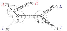
Figure 1: Example of the HELAS algorithm. Helicity amplitudes are calculated by iteratively combining particles to off-shell particles/wavefunctions. In the above case, particle 1 and 2 would be combined to a new off-shell fermion in vertex (1), and gluon 3 and 4 would be combined to one new particle in vertex (2). These two off-shell particles would merge with particle 5 in the last vertex (3).

Every intermediate state (constructed in a vertex combining two or three existing, on- or off-shell, particles) is numerically evaluated as an off-shell wavefunction which feeds into the rest of the calculation. Eventually three or four (on- or off-shell) particles may join in a vertex, to create the amplitude corresponding to the Feynman diagram in question. We will refer to this algorithm as the HELAS algorithm.

In line with previous work (Lifson:2022ijv, ) this structure is maintained in the current chirality-flow implementation, immediately enabling the same level of (off-shell) wavefunction recycling as in standalone MadGraph5_aMC@NLO, as well as a transparent speed comparison, where it is ensured that any speedgain comes either from the simplified Lorentz structures or from the use of reference and spin vectors. Consequently, there are only two major changes made in our implementation:

• Rather than exporting ALOHA-generated (HELAS-like) code, subroutines are called from a rewritten flow-based version of the HELAS library, which makes use of the simplified chirality-flow Lorentz structures in the numerical evaluation of propagators and amplitudes.

• The diagram generation routine is modified to account for particles with definite chiral (or spin) states. In particular, chiral massless fermions are introduced, and external gauge bosons are supplied with a reference vector (cf. eq. (2.1.7)), allowing for gauge based Feynman and chirality-flow diagram removal already at code generation time.

Compared to the default MadGraph5_aMC@NLO implementation this implies simplifications which in essence appear at two different levels:

• Simplified Lorentz structures: Chirality flow makes subroutines smaller than the corresponding routines in e.g. HELAS. This applies in particular to vertices with chiral fermions, but even massive fermion vertices are less computationally demanding.

• Gauge based Feynman or chirality-flow diagram removal: The numerical evaluation is simplified further by the choice of reference momenta and spin axes, as contributions may be known to vanish already at code generation time. This reduces the computation length, either directly at the Feynman diagram generation level (as some vertices and thereby Feynman diagrams may vanish), or at the level of chirality-flow diagrams (since chirality-flow diagrams which are known to evaluate to 0 can be ignored). For example, the kinematic factor multiplying one of the color structures in the four-gluon vertex may vanish. These simplifications are further described in section 4, and they provide acceleration primarily to the gluon-only vertices and the massless fermion-vector vertex.

3.1 Arrow direction for the HELAS algorithm

As discussed in section 2.4, the choice of flow direction is simple for pen and paper calculations. For automated algorithms, however, it is necessary to ensure that a consistent choice of chirality flow can be set not just for a single chirality-flow diagram, but for all possible chirality-flow diagrams, while working at the level of single vertices. Hence, a convention which can be translated to a simple algorithmic choice must be used.

Instead of assigning chirality-flow direction for each diagram individually, we therefore use the convention that all left-chiral spinors are treated as having inflowing chirality (i.e. they are given by a left-chiral bra $\color[rgb]{0,0,1}{{\color[rgb]{0,0,1}[}|}$) whereas right-chiral spinors are considered outflowing (i.e. they are given by a right-chiral ket $\color[rgb]{1,0,0}{|{\color[rgb]{1,0,0}\rangle}}$). The same convention is applied to gauge bosons, but we note that while external gauge bosons can be treated as direct products of left- and right-chiral spinors (cf. eq. (2.1.7)), internal propagators require a description in terms of a matrix ($\sim M_{{\alpha}{\dot{\beta}}}$) due to the presence of the triple-gluon vertex and contributions from more than one term. For simplicity, we therefore represent all gluons in this form.

With these conventions, spinor inner products are always constructed from spinors of the same form (i.e. a bra with a bra and a ket with a ket). As an example, the second chirality-flow diagram in eq. (2.3.3) is mapped to the arrow assignment

    (in code) (3.1.1)

in our HELAS algorithm (figure 1). Contractions then have to include systematic multiplication with the Levi-Civita tensor to align the flows, i.e., always contract an upper spinor index with a lower. Since the ALOHA code is written in component form, this implies no speed loss.

4 Gauge specific Feynman rules and simplifications from spin-direction

In this section we explore how knowledge of chirality and spin can be used to define gauge dependent Feynman rules, and how these can be exploited in the context of the HELAS algorithm. Although, clearly, the gluon reference vectors can be chosen independently for each external gauge boson (for example, for a gluon with momentum $(p^{0},\vec{p})$, the custom choice is $(p^{0},-\vec{p})$), there are advantages with choosing them similarly for all left- and right-chiral gluons respectively, as this gives rise to the vanishing of more contractions. We therefore limit our study to gauge choices where all external gluons of the same chirality have the same reference vector, which we further take to equal some other spinor occurring in the process.

For internal gluons, the flow representation will make it transparent how to deduce information about their spinor structure. For example, the off-shell gluon arising in vertex 2 in figure 1 will necessarily come with the reference vector $r_{L}$ in its right-chiral spinor, as seen from eq. (2.3.3). This means that we need to distinguish four different types of gluons, left-chiral $g_{L}$, right-chiral $g_{R}$, general $g$ (i.e. no specific knowledge of spinor structure), and gluons which are used for setting the reference momentum of opposite-chirality gluons, $g_{LR}$ (or internal gluons which inherit this spinor structure). These gluons behave both as left- and right-chiral gluons in the contractions.

A left-chiral gluon thus comes with a spinor structure ${\color[rgb]{1,0,0}|}r_{L}{\color[rgb]{1,0,0}\rangle}{\color[rgb]{0,0,1}[}p_{g}{\color[rgb]{0,0,1}|}$ in the code (generally alternatively ${\color[rgb]{0,0,1}|}p_{g}{\color[rgb]{0,0,1}]}{\color[rgb]{1,0,0}\langle}r_{L}{\color[rgb]{1,0,0}|}$), and a right-chiral gluon comes with ${\color[rgb]{1,0,0}|}p_{g}{\color[rgb]{1,0,0}\rangle}{\color[rgb]{0,0,1}[}r_{R}{\color[rgb]{0,0,1}|}$ in the code (or generally ${\color[rgb]{0,0,1}|}r_{R}{\color[rgb]{0,0,1}]}{\color[rgb]{1,0,0}\langle}p_{g}{\color[rgb]{1,0,0}|}$), whereas $g_{LR}$-gluons come with ${\color[rgb]{1,0,0}|}r_{L}{\color[rgb]{1,0,0}\rangle}{\color[rgb]{0,0,1}[}p_{g}=r_{R}{\color[rgb]{0,0,1}|}$ or ${\color[rgb]{1,0,0}|}p_{g}=r_{L}{\color[rgb]{1,0,0}\rangle}{\color[rgb]{0,0,1}[}r_{R}{\color[rgb]{0,0,1}|}$ in the code (or generally ${\color[rgb]{0,0,1}|}p_{g}=r_{R}{\color[rgb]{0,0,1}]}{\color[rgb]{1,0,0}\langle}r_{L}{\color[rgb]{1,0,0}|}$ or ${\color[rgb]{0,0,1}|}r_{R}{\color[rgb]{0,0,1}]}{\color[rgb]{1,0,0}\langle}p_{g}=r_{L}{\color[rgb]{1,0,0}|}$). Here we note that $p_{g}$ is the momentum of the gluon for an external gluon, but is an “inherited” momentum entering as a spinor argument for an internal gluon. The inherited spinor structure can be exploited for subsequent simplifications “further in” in the Feynman diagram, and we will refer to gluons carrying the spinors ${\color[rgb]{1,0,0}|}r_{L}{\color[rgb]{1,0,0}\rangle}$ and ${\color[rgb]{0,0,1}[}r_{R}{\color[rgb]{0,0,1}|}$ as effectively chiral.

If we consider a process with only gluons, it is clear that picking the reference momentum $r_{L}$ of the left-chiral gluons to equal the momentum of a right-chiral gluon, additional spinor contractions vanish, implying additional simplifications. For processes with both quarks and gluons it is less obvious if the most advantageous choice is to set the reference vector after a right-chiral gluon or after a right-chiral quark, something we discuss further in section 4.4.

For massive particles, the corresponding degree of freedom becomes physical, and is related to the direction in which spin is measured, but we can still use the freedom to measure spin in any direction to shorten the calculations. We discuss this further in section 4.5. Beyond simplifications obvious from the chirality flow, we explore how the Schouten identity can be used to further simplify the four-gluon vertex.

For the purpose of the HELAS algorithm, as discussed in section 3, we need to distinguish between vertices resulting in off-shell particles (wavefunctions) and vertices resulting in amplitudes. At the first steps of the HELAS algorithm we have external gluons with manifest helicities. However, we will see that the internal (off-shell) gauge bosons often end up being effectively chiral.

4.1 The triple-gluon vertex

We first consider the chiral structure of the three-gluon vertex,

$$\includegraphics[scale={0.35},valign={c}]{Jaxodraw/QCDPaper/3g1}\!\!\!\quad+\includegraphics[scale={0.35},valign={c}]{Jaxodraw/QCDPaper/3g2}\!\!\!\quad+\includegraphics[scale={0.35},valign={c}]{Jaxodraw/QCDPaper/3g3}\!\!\!,$$ (4.1.1)

assuming that all left-chiral gluons have the same reference momentum, and similarly for all right-chiral gluons. It is then immediately obvious that a vertex between three gluons with equal chirality vanishes as the directly connected double line gives ${\color[rgb]{0,0,1}[}r_{\color[rgb]{1,0,0}R}|r_{\color[rgb]{1,0,0}R}{\color[rgb]{0,0,1}]}$ or ${\color[rgb]{1,0,0}\langle}r_{\color[rgb]{0,0,1}L}|r_{\color[rgb]{0,0,1}L}{\color[rgb]{1,0,0}\rangle}$ for all three terms, for example

$$\underbrace{\includegraphics[scale={0.35},valign={c}]{Jaxodraw/QCDPaper/3g1LLL}}_{\propto\,{\color[rgb]{1,0,0}\langle}r_{\color[rgb]{0,0,1}{L}}r_{\color[rgb]{0,0,1}{L}}{\color[rgb]{1,0,0}\rangle}\,=\,0}\!\!\!\quad+\underbrace{\includegraphics[scale={0.35},valign={c}]{Jaxodraw/QCDPaper/3g2LLL}}_{\propto\,{\color[rgb]{1,0,0}\langle}r_{\color[rgb]{0,0,1}{L}}r_{\color[rgb]{0,0,1}{L}}{\color[rgb]{1,0,0}\rangle}\,=\,0}\!\!\!\quad+\underbrace{\includegraphics[scale={0.35},valign={c}]{Jaxodraw/QCDPaper/3g3LLL}}_{\propto\,{\color[rgb]{1,0,0}\langle}r_{\color[rgb]{0,0,1}{L}}r_{\color[rgb]{0,0,1}{L}}{\color[rgb]{1,0,0}\rangle}\,=\,0}\;.$$ (4.1.2)

Similarly, if two of the gluons share a known chirality, say left, the term where the two left-chiral gluons are contracted vanishes and only two terms remain.

Now consider vertices with $g_{LR}$. This effectively left-right gluon will induce all of the simplifications for left and right gluons above, for example in the $g_{L}\,g_{R}\,g_{LR}$ vertex, where with $g_{1}=g_{L}$, $g_{2}=g_{R}$, and $g_{3}=g_{LR}$ two out of three chiral structures are removed,

$$\includegraphics[scale={0.35},valign={c}]{Jaxodraw/QCDPaper/3g1L_R_LR}\!\!\!\quad+\underbrace{\includegraphics[scale={0.35},valign={c}]{Jaxodraw/QCDPaper/3g2L_R_LR}}_{\propto\,{\color[rgb]{0,0,1}[}r_{\color[rgb]{1,0,0}R}r_{\color[rgb]{1,0,0}R}{\color[rgb]{0,0,1}]}\,=\,0}\!\!\!\quad+\underbrace{\includegraphics[scale={0.35},valign={c}]{Jaxodraw/QCDPaper/3g3L_R_LR}}_{\propto\,{\color[rgb]{1,0,0}\langle}r_{\color[rgb]{0,0,1}L}r_{\color[rgb]{0,0,1}L}{\color[rgb]{1,0,0}\rangle}\,=\,0}\!\!\!.$$ (4.1.3)

Similarly a vertex between the left and right reference gluon will always vanish since if say $g_{1}=g_{L}$, $g_{2}=g_{R}$ and $r_{R}=p_{1}$, $r_{L}=p_{2}$, the first term vanishes immediately, whereas, for external $g_{1}$ and $g_{2}$, the second and third term vanishes by contractions with the momentum-dot using momentum conservation,

$$\underbrace{\includegraphics[scale={0.35},valign={c}]{Jaxodraw/QCDPaper/3g1LRLR}}_{\propto\,{\color[rgb]{0,0,1}[}p_{1}\,p_{1}\,{\color[rgb]{0,0,1}]}=0,\;{\color[rgb]{1,0,0}\langle}p_{2}p_{2}{\color[rgb]{1,0,0}\rangle}\,=\,0}\!\!\!\quad+\underbrace{\includegraphics[scale={0.35},valign={c}]{Jaxodraw/QCDPaper/3g2LRLR}}_{0}\!\!\!\quad+\underbrace{\includegraphics[scale={0.35},valign={c}]{Jaxodraw/QCDPaper/3g3LRLR}}_{0}\;,$$ (4.1.4)

since $p_{2}-p_{3}=2p_{2}+p_{1}$ giving $2{\color[rgb]{1,0,0}\langle}p_{2}\,p_{2}{\color[rgb]{1,0,0}\rangle}{\color[rgb]{0,0,1}[}p_{2}p_{1}{\color[rgb]{0,0,1}]}+{\color[rgb]{1,0,0}\langle}p_{2}\,p_{1}{\color[rgb]{1,0,0}\rangle}{\color[rgb]{0,0,1}[}p_{1}p_{1}{\color[rgb]{0,0,1}]}=0$, etc. Therefore the external reference gluons can never couple directly to each other.

For the $g\,g_{L}\,g_{R}$-vertex, $g_{L}$ and $g_{R}$ contract to each other as if they were unpolarized, implying that there is no gain to be found in this case (unless one of them is a reference gluon, $g_{LR}$). Similarly there is no simplification for vertices with no or only one gluon with known chirality. A systematic treatment of all versions of the triple-gluon vertex is given in appendix B.

4.1.1 Vertices resulting in off-shell wavefunctions

In the context of the HELAS algorithm, we note that the above treatment, with three gluons of (potentially) known chirality, is only applicable to the last step, where three gluons result in an amplitude. For the other steps, the created off-shell gluon will a priori be of unknown chirality, and we rather want to derive information about its chiral structure. Thus we need to consider two (on- or off-shell) gluons, $g_{1}$ and $g_{2}$ of (potentially) known chirality, coming into a vertex which results in a third off-shell gluon with derived chiral structure.

If both $g_{1}$ and $g_{2}$ are left-chiral, we have

$$\underbrace{\includegraphics[scale={0.35},valign={c}]{Jaxodraw/QCDPaper/3g1LLV}}_{\propto\,{\color[rgb]{1,0,0}\langle}r_{\color[rgb]{0,0,1}{L}}r_{\color[rgb]{0,0,1}{L}}{\color[rgb]{1,0,0}\rangle}\,=\,0}\!\!\!\quad+\includegraphics[scale={0.35},valign={c}]{Jaxodraw/QCDPaper/3g2LLV}\!\!\!\quad+\includegraphics[scale={0.35},valign={c}]{Jaxodraw/QCDPaper/3g3LLV}\!\!\!\quad,$$ (4.1.5)

where the first term disappears due to the contraction between the (right-chiral) reference spinors for left-chiral gluons. From the above spinor structure, we also deduce that the off-shell gluon will effectively be left-chiral, i.e., when two gluons of the same chirality enter a three-gluon vertex, the resulting propagator will also act as having a well-defined chiral structure, which may continue to lead to further simplifications further inside the Feynman diagram. For example, the off-shell internal gluon resulting in vertex (2) in figure 1 will be effectively left-chiral.

Next, assume that $g_{1}$ and $g_{2}$ have opposite chirality, say $g_{1}$ left and $g_{2}$ right. Then, generally, none of the terms in eq. (4.1.1) disappear, and the resulting off-shell gluon can neither be treated as left nor right. However, if we set e.g. the right-chiral reference momentum to be the momentum of $g_{1}$ (which thus must be an external gluon), $r_{R}=p_{1}$, and thereby make $g_{1}$ act as “doubly chiral” $g_{LR}$, we find

$$\underbrace{\includegraphics[scale={0.35},valign={c}]{Jaxodraw/QCDPaper/3g1RefLRV}}_{\propto\,{\color[rgb]{0,0,1}[}p_{1}\,p_{1}{\color[rgb]{0,0,1}]}\,=\,0}\!\!\!\quad+\underbrace{\includegraphics[scale={0.35},valign={c}]{Jaxodraw/QCDPaper/3g2RefLRV}}_{\text{effectively right-chiral}}\!\!\!\quad+\underbrace{\includegraphics[scale={0.35},valign={c}]{Jaxodraw/QCDPaper/3g3RefLRV}}_{=\,0,\text{ (if also $g_{2}$ external)}}\!\!\!,$$ (4.1.6)

where, for external $g_{2}$, the third term disappears due to contractions in the momentum-dot. Regardless of whether $g_{2}$ is external or not, the resulting gluon will effectively act as right-chiral in further vertices.

If $r_{R}\neq p_{1}$, but $r_{L}=p_{2}$ in eq. (4.1.6), s.t. $g_{2}=g_{LR}$, the propagating gluon would instead act as left-chiral. Additionally, if $g_{1}=g_{LR}$ and $g_{2}=g_{LR}$, all three terms vanish by momentum conservation for external gluons. A systematic treatment of all versions of the vertex is given in appendix B.

4.2 The four-gluon vertex

Next, we turn to the four-gluon vertex, which comes with three chiral structures multiplying three different color structures

$$if^{a_{1}a_{2}b}if^{ba_{3}a_{4}}\left(\includegraphics[scale={0.225},valign={c}]{Jaxodraw/MS/4GluonVertexV2_Kin13}-\includegraphics[scale={0.225},valign={c}]{Jaxodraw/MS/4GluonVertexV2_Kin14}\right)+if^{a_{1}a_{3}b}if^{ba_{4}a_{2}}\left(\includegraphics[scale={0.225},valign={c}]{Jaxodraw/MS/4GluonVertexV2_Kin14}-\includegraphics[scale={0.225},valign={c}]{Jaxodraw/MS/4GluonVertexV2_Kin12}\right)$$

$$+if^{a_{1}a_{4}b}if^{ba_{2}a_{3}}\left(\includegraphics[scale={0.225},valign={c}]{Jaxodraw/MS/4GluonVertexV2_Kin12}-\includegraphics[scale={0.225},valign={c}]{Jaxodraw/MS/4GluonVertexV2_Kin13}\right)~{},$$ (4.2.1)

where we remark that the gluons which are contracted in color are not contracted in the chiral structure.

We first note that this vertex vanishes fully whenever three (or four) gluons share the same chirality. By considering eq. (4.2.1), but taking two gluons to be general, while keeping two gluons left (same chirality), we immediately see that one of the three spinor contractions vanishes. For three or four general gluons, or for two gluons of opposite chirality, no simplifications arise, whereas four-gluon vertices with $g_{LR}$ may result in many vanishing terms since these gluons can neither be contracted with $g_{L}$ nor $g_{R}$. For example the vertex $g_{LR}g_{L}g_{R}g$ only has one surviving spinor contraction since $g_{LR}$ must be contracted with $g$ for a non-vanishing result.

Additionally, we note that further simplifications can be obtained by exploiting the Schouten identity, which in the flow picture can be represented as

$$\underbrace{\includegraphics[scale={0.45},valign={c}]{Jaxodraw/MS/SchoutenHorSolidCol}}_{{\color[rgb]{1,0,0}\langle}ij{\color[rgb]{1,0,0}\rangle}{\color[rgb]{1,0,0}\langle}kl{\color[rgb]{1,0,0}\rangle}} =\underbrace{\includegraphics[scale={0.45},valign={c}]{Jaxodraw/MS/SchoutenCrossSolidCol}}_{{\color[rgb]{1,0,0}\langle}ik{\color[rgb]{1,0,0}\rangle}{\color[rgb]{1,0,0}\langle}jl{\color[rgb]{1,0,0}\rangle}}+\underbrace{\includegraphics[scale={0.45},valign={c}]{Jaxodraw/MS/SchoutenVertSolidCol}}_{{\color[rgb]{1,0,0}\langle}il{\color[rgb]{1,0,0}\rangle}{\color[rgb]{1,0,0}\langle}kj{\color[rgb]{1,0,0}\rangle}}~{},$$ (4.2.2)

and similarly for left-chiral spinors. Applying this to the four-gluon vertex yields simplifications beyond those immediately apparent from the flow. As an example, consider the $g_{L}g_{L}g_{R}g_{R}$-vertex (again with the particle positions from eq. (4.2.1)), and apply the Schouten identity

$$\includegraphics[scale={0.25},valign={c}]{Jaxodraw/MS/4GluonVertexLLRR_Kin13Sch}=-\underbrace{\includegraphics[scale={0.225},valign={c}]{Jaxodraw/MS/4GluonVertexLLRR_Sch1}}_{\text{0}}+\includegraphics[scale={0.25},valign={c}]{Jaxodraw/MS/4GluonVertexLLRR_Sch2}=-\underbrace{\includegraphics[scale={0.225},valign={c}]{Jaxodraw/MS/4GluonVertexLLRR_Sch4}}_{0}+\includegraphics[scale={0.25},valign={c}]{Jaxodraw/MS/4GluonVertexLLRR_Sch3}\;.$$ (4.2.3)

Thus two of the chiral structures in eq. (4.2.1) are equal and need only be evaluated once. We therefore see that the chiral structures multiplying the first color structure cancel by the Schouten identity. On top of that, the chirality flow with vertical lines immediately vanishes, implying that the two remaining color factors in eq. (4.2.1) multiply the same kinematic amplitude.

4.2.1 Vertices resulting in off-shell wavefunctions

We now consider vertices resulting in an off-shell gluon, assuming that $g_{4}$ will be the returned off-shell particle. Assume first that $g_{1}$ and $g_{2}$ have the same chirality, e.g $g_{1}$ and $g_{2}$ are both left-chiral whereas $g_{3}$ is right-chiral. Then (keeping the same gluon positions as above) we have

$$if^{a_{1}a_{2}b}if^{ba_{3}a_{4}}\left(\underbrace{\includegraphics[scale={0.225},valign={c}]{Jaxodraw/MS/4GluonVertexOffLLR_Kin13}-\includegraphics[scale={0.225},valign={c}]{Jaxodraw/MS/4GluonVertexOffLLR_Kin14}}_{\text{left}}\right)+if^{a_{1}a_{3}b}if^{ba_{4}a_{2}}\left(\underbrace{\includegraphics[scale={0.225},valign={c}]{Jaxodraw/MS/4GluonVertexOffLLR_Kin14}}_{\text{left}}-\underbrace{\includegraphics[scale={0.225},valign={c}]{Jaxodraw/MS/4GluonVertexOffLLR_Kin12}}_{0}\right)$$

$$+if^{a_{1}a_{4}b}if^{ba_{2}a_{3}}\left(\underbrace{\includegraphics[scale={0.225},valign={c}]{Jaxodraw/MS/4GluonVertexOffLLR_Kin12}}_{0}-\underbrace{\includegraphics[scale={0.225},valign={c}]{Jaxodraw/MS/4GluonVertexOffLLR_Kin13}}_{\text{left}}\right)~{},$$ (4.2.4)

i.e. the propagator resulting from a vertex with two gluons of the same (effective) chirality will also have a definite effective chirality. Since external particles have a well-defined chirality, ambiguity in the internal chiral states of gauge bosons arises only from quark-gluon and three-gluon vertices.

We leave out the details here, but for vertices with only one chiral gluon or with two gluons of opposite chirality, no simplifications arise, whereas further simplifications arise for the $g_{LR}$ gluons. In total, identifying chiralities of internal gluons and applying Schouten identities allows for extensive gauge based (chirality-flow) diagram removal. Again we leave out further details here, but provide the number of remaining kinematic terms for the different chiral configurations ($g_{LR}$, $g_{L}$, $g_{R}$ and $g$) in appendix B.

We also remark that the three spinor contractions multiplying different color structures, have to be treated independently for further steps in the HELAS algorithm.

4.3 The fermion-gluon vertex

The final vertex we treat is the fermion-gauge boson vertex, for which we consider the case of a massless and a massive fermion separately. For massless quarks, we always have a well-defined chiral state, while for massive fermions we can explore the freedom to choose spin direction in such a way that at least some chirality-flow diagrams vanish.

4.4 The massless fermion-gluon vertex

The (massless) fermion-gluon vertex has the structure of

(4.4.1)

from which it is immediately clear that if one of the spinors of the gluon matches one of the spinors of the quark, the vertex will vanish. This will happen for example if the gluon is right-chiral and has the quark momentum $p_{1}$ as reference momentum, ${\color[rgb]{0,0,1}[}p_{1}|g_{L}=r_{R}=p_{1}{\color[rgb]{0,0,1}]}=0$. This is in direct analogy to QED in eq. (2.3.1), where right-chiral photons can not attach to the left-chiral reference fermion. While we could alternatively set the gluon reference momenta according to the momenta of other gluons, setting them to the momenta of quarks turns out to give the best speedgain for high multiplicities, as some vertices — and thereby Feynman diagrams — can be fully removed, rather than (typically) just be simplified, as in the gluon-only case.

4.4.1 Vertices resulting in off-shell wavefunctions

As for the gluon vertices, we need to distinguish vertices resulting in off-shell wavefunctions from vertices resulting in amplitudes for the purpose of the HELAS algorithm. If the vertex results in an off-shell fermion we have one of the situations

$$\includegraphics[scale={0.4},valign={c}]{Jaxodraw/QCDPaper/gqRinp}\quad\text{or}\quad\includegraphics[scale={0.4},valign={c}]{Jaxodraw/QCDPaper/gqLinp}\;,$$ (4.4.2)

where we also display the momentum-dot coming from the massless fermion propagator.

We note that if the gluon and the external quark share a spinor, the contraction vanishes. Again this will only happen if the gluon has the quark momentum as reference spinor. If the diagram does not vanish, the fermion continues in to a fermion propagator containing a momentum-dot. The end of that propagator will then again have an explicit chirality (the same chirality as the original incoming quark), while entering the next vertex (gray blob above). The quark thus remains chiral. Technically this momentum-dot is included in the vertex implementation.

If instead, the fermions give an off-shell gluon, we note that the gluon can be effectively chiral if one of the fermion momenta is used for the gluon reference momentum.

4.5 Massive fermions with general spin direction

As discussed in section 2.1 we may explore the freedom of choosing the spin axis $s^{\mu}$ to our benefit, such that some chirality-flow diagrams vanish. We recall that the spin operator is defined as (see e.g. Ohlsson:2011zz ),

$$\frac{1}{2}\Sigma^{\mu}=-\frac{1}{4m}\epsilon^{\mu\nu\lambda\omega}P_{\nu}\sigma_{\lambda\omega}~{},$$ (4.5.1)

where $P_{\nu}$ is the momentum operator ($P_{\nu}=i\partial/\partial x^{\nu}$), $\epsilon^{\mu\nu\lambda\omega}$ ($\epsilon^{0123}\equiv 1\Rightarrow\epsilon_{0123}=-1$) is the four-dimensional Levi-Civita tensor, and $\sigma^{\mu\nu}$ (giving the Lorentz generators for the $(1/2,1/2)$-representation) is defined as

$$\sigma^{\mu\nu}=\frac{i}{2}\left[\gamma^{\mu},\gamma^{\nu}\right]~{}.$$ (4.5.2)

The spin projected onto $s^{\mu}$ is then given by the operator

$$\mathcal{O}_{s}=-\frac{\Sigma^{\mu}s_{\mu}}{2}=\frac{1}{4m}\epsilon^{\mu\nu\lambda\omega}s_{\mu}P_{\nu}\sigma_{\lambda\omega}~{},$$ (4.5.3)

such that the spin direction, in this sense, is actually only defined up to a four-momentum proportional to the particle’s momentum $p$. Adding any linear combination of $p$ to $s=(1/m)\left(p-2\alpha q\right)$ (eq. (2.1.5)) will result in the same $\mathcal{O}_{s}$. Therefore, we could equally well have used $s^{\prime}=-2\alpha q/m=-mq/(p\cdot q)$ for the spin direction. Thus $q$ plays the role of defining the other four-vector (aside from $p$) which determines the operator $\mathcal{O}_{s}$, and thereby what we mean with positive and negative spin.

This we will use to our advantage. While the direction $s=(1/m)\left(p-2\alpha q\right)$ clearly depends on the particle’s momentum, the momentum $q$ can be taken to be the same for all particles. For further simplifications, we may choose it to be the same as the momentum for some other spinor in the process, such as for example the reference vector of left-chiral gluons.

4.6 The massive fermion-gluon vertex

The structure of the massive fermion vertex (itself) contains the flows

and (4.6.1)

for some spinors, for external fermions either ${\color[rgb]{0,0,1}[}p_{L}{\color[rgb]{0,0,1}|}={\color[rgb]{0,0,1}[}q{\color[rgb]{0,0,1}|}$ and ${\color[rgb]{1,0,0}\langle}p_{R}{\color[rgb]{1,0,0}|}={\color[rgb]{1,0,0}\langle}p^{\flat}{\color[rgb]{1,0,0}|}$ or ${\color[rgb]{0,0,1}[}p_{L}{\color[rgb]{0,0,1}|}={\color[rgb]{0,0,1}[}p^{\flat}{\color[rgb]{0,0,1}|}$ and ${\color[rgb]{1,0,0}\langle}p_{R}{\color[rgb]{1,0,0}|}={\color[rgb]{1,0,0}\langle}q{\color[rgb]{1,0,0}|}$, as given in eqs. (A.0.1) and (A.0.4) in appendix A (and accompanied by the phases and factors stated there).

As in eq. (4.4.1), we may thus remove vertices with for example ${\color[rgb]{0,0,1}[}p_{L}=q=r_{R}|g_{L}=r_{R}{\color[rgb]{0,0,1}]}$ if $p_{L}$ is set to equal the reference spinor of the right-chiral gluons. This momentum ($r_{R}$) may in turn be taken to equal the physical momentum of a left-chiral gluon.

Alternatively the reference vector $r_{R}$ of all right-chiral gluons may be put to equal the $p^{\flat}$ vector of some quark. For a low number of gluons this will lead to many vanishing chirality-flow diagrams, since the reference quark can not couple to one of the gluons. However the number of terms that can be removed in this way scales badly with the number of gluons. Overall, we have rather found it advantageous to let the physical momentum of an opposite-chirality gluon dictate the vector $q$ for the quarks, with $q=r_{L}/r_{R}=p_{\text{some right/left gluon}}$.

With this choice, the full vertex will never vanish, but for processes with many gluons, it turns out to give the best overall speedup, due to the simplifications in the gluon vertices. We remark that this is contrary to the situation with massless quarks, where the best high-multiplicity speedup is found by setting the reference momenta to be the momentum of a quark (with opposite chirality). From this, it is clear that (for example) if the left gluon spinor equals ${\color[rgb]{0,0,1}|}p_{L}{\color[rgb]{0,0,1}]}$ the first part of the vertex disappears, but the second term remains.

4.6.1 Vertices resulting in off-shell wavefunctions

In general, for a vertex resulting in an off-shell fermion wavefunction, we have terms of the form

,,

and, (4.6.2)

where, like in the massless case, we choose to include the chiral structure of the propagator, to get the spinor structure entering the next vertex.

In general all four such terms may survive, but again, if the gluon spinor contracted with the incoming quark is given by the same momentum $p_{L}$ or $p_{R}$, two of the terms above will vanish, which is used to build faster versions of the code. However, due to the massive propagator, the simple structure of one outgoing helicity is nevertheless lost for the fermion entering the next vertex. In spite of this, our representation of the fermion-gauge boson vertices are less computationally demanding.

Finally, we note that the vertex may alternatively result in an off-shell gluon, which then is of general type $g$.

5 Results

In this section, we present time measurements for amplitude evaluations in the chirality-flow implementation, and comparisons to the standalone version of MadGraph5_aMC@NLO. Since we use the same diagram generation and code generation routines as the native MadGraph5_aMC@NLO  framework, and only (i) speed up numerical subroutines using a flow-based library, and (ii) remove (chirality-flow) diagrams known not to contribute, we are confident that any improvement in performance can be attributed entirely to chirality flow. Since we only address the Lorentz structure, the squaring of the color structure has been turned off for both versions of the code, to assess the speedup of the Lorentz structure. This would otherwise be a bottleneck for high multiplicities.

We first explore the speedup in the pure Yang-Mills case. Then, bearing in mind that almost all fermions are effectively massless at LHC energies, we consider massless up quarks. Finally we explore gluon induced $t\bar{t}$ production in association with up to three additional gluons. In all cases we find an increasing speedgain with increasing multiplicity.

Time measurements were made on a MacBook Pro laptop with an Intel Core i7-4980HQ CPU and runtime measurements are taken over 100 000 randomly generated phase space points. At present, our code generates each chirality/spin configuration as a different runtime process, and phase space points are hence generated with RAMBO Kleiss:1985gy separately for each spin configuration for chirality flow, whereas this is done outside the spin sum for MadGraph5_aMC@NLO. For high multiplicities, the runtime for RAMBO is negligible, but for small multiplicities this overhead slows down our implementation. Even so, we find for all processes that the chirality-flow implementation outperforms MadGraph5_aMC@NLO  already for five external particles.

It should be noted that our results are from the standalone version. For helicity sampling, we expect them to carry over to the full version, but it should be noted that since recently MadGraph5_aMC@NLO  comes with helicity recycling, where parts of Feynman diagrams are recycled between processes with different helicities Mattelaer:2021xdr . This can be applied to our version as well. However some adjustment would be needed, since to fully exploit helicity recycling, one needs to use the same reference vectors ($r_{L}$ and $r_{R}$) for all helicity configurations, whereas we have chosen them differently. Picking different $r_{L}/r_{R}$ for different helicities will result in some speed loss, although the bulk of the improvement will remain.

5.1 Gluon processes

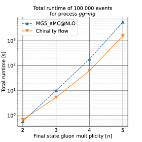
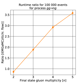
Figure 2: Runtimes (left) and ratio (right) for $gg\rightarrow ng$ for standalone MadGraph5_aMC@NLO and for the chirality-flow branch of the code. The squaring of the color structure has been turned off to compare only the Lorentz structure treatment. In the current chirality-flow implementation, the RAMBO momentum sampling is done separately for each spin configuration, and this overhead has a runtime impact for low multiplicities. The amplitude evaluations themselves are consistently faster for chirality flow, but this code artifact outweighs the acceleration at multiplicity four. For high multiplicities, the phase space sampling takes a negligible fraction of the total runtime.

We here explore the benefits of chirality flow in the pure gluon case, $gg\rightarrow ng$, $n=2\ldots 5$. Our reference vectors are set as discussed in section 4, i.e., left-chiral gluons with a reference vector for the right spinor are treated as ${\color[rgb]{1,0,0}|}r_{L}{\color[rgb]{1,0,0}\rangle}{\color[rgb]{0,0,1}[}p_{g}{\color[rgb]{0,0,1}|}$, where the reference vector $r_{L}$ is taken to be the same for all left gluons. Further, it is taken to equal the momentum of a right-chiral gluon (the right-chiral gluon with lowest number in MadGraph5_aMC@NLO). Reference vectors for right-chiral gluons are set similarly.

Runtime comparisons are shown in figure 2. We note that there is an increased speedup for high multiplicity. This speedgain can be attributed to a high number of vanishing chirality-flow diagrams when the vanishing of ${\color[rgb]{0,0,1}[}r_{R}{\color[rgb]{0,0,1}|}r_{R}{\color[rgb]{0,0,1}]}$, ${\color[rgb]{0,0,1}[}p_{\text{ref}}=r_{R}{\color[rgb]{0,0,1}|}r_{R}{\color[rgb]{0,0,1}]}$, ${\color[rgb]{1,0,0}\langle}r_{L}{\color[rgb]{1,0,0}|}r_{L}{\color[rgb]{1,0,0}\rangle}$ and ${\color[rgb]{1,0,0}\langle}\tilde{p}_{\text{ref}}=r_{L}{\color[rgb]{1,0,0}|}r_{L}{\color[rgb]{1,0,0}\rangle}$, but also the Schouten identity, is used. As detailed in appendix B, this leads to many vanishing chirality-flow terms. However, as opposed to the case of the (massless) fermion-gauge boson vertex (cf. ref. Lifson:2022ijv and section 5.2 below), there is no speedup in the vertex subroutines themselves, which are comparable in number of instructions to the native MadGraph5_aMC@NLO  implementation (as measured using Valgrind Nethercote:2007vaf ; Weidendorfer:2004ccs ).

5.2 Processes with massless quarks

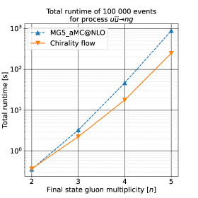
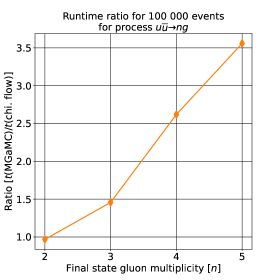
Figure 3: Runtime (left) and ratio (right) for the Lorentz structure for $u\bar{u}\rightarrow ng$ for the standalone version of MadGraph5_aMC@NLO  and for the chirality-flow branch, cf. figure 2.

We next address amplitudes with one $q\bar{q}$ pair. As discussed in section 4.4, we have found it advantageous (for high multiplicities) to set reference momenta according to the quarks, since this allows for the removal of all diagrams where any left-chiral gluon is attached to the right-chiral reference quark, and similarly for right-chiral gluons attached to the left-chiral reference quark.

In figure 3 we display our results for $u\bar{u}\rightarrow ng$ (again with the squaring of color turned off, although here this effect is only sizable for the five-gluon case). As for the pure Yang-Mills case, we find an increased speedgain for high multiplicities, but as opposed to the the gluon case, this is not only due to the gauge based (chirality-flow) diagram removal, but also due to the compact nature of the fermion-gauge boson vertex, as in ref. Lifson:2022ijv .

5.3 Processes with massive quarks

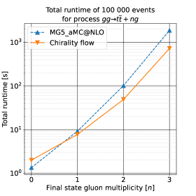
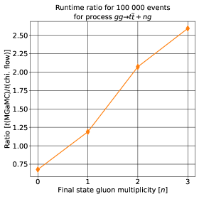
Figure 4: Runtime (left) and ratio (right) for the Lorentz structure of $gg\rightarrow t\bar{t}+ng$, for standalone MadGraph5_aMC@NLO  and for the chirality-flow version of it, cf. figure 2.

As described in section 4 we here have two kinds of vectors to choose: The unphysical reference vectors of the gluons (which may in principle be picked differently for processes with different fermion spins) and the physical vector $q$, related to the spin direction as described in section 4.5.

The reference vector of a gluon can thus be set according to the momentum of another gluon (as in the gluon-only case) or according to one of the two spinors describing a massive quark. In the latter case, we note that — as opposed to for massless quarks — this will not remove the entire vertex (and thereby Feynman diagram), but will only remove one chirality-flow configuration. In the massive fermion case we have therefore found it advantageous to set the reference momenta of the gluons according to the momentum of a gluon with opposite chirality (as for the pure Yang-Mills case). The physical reference vector for the quarks ($q$) is then set to equal the most frequently occurring gluon reference vector.

The exception to this is when all gluons have the same chirality. In this case, the momentum $q$ for the quarks is set to equal one gluon momentum, and the gluon reference momenta (all $r_{L}$ or $r_{R}$) are set to equal the $p^{\flat}$ of the same quark.

A runtime comparison between the standalone version of MadGraph5_aMC@NLO  and its chirality-flow branch is shown in figure 4. Despite that this represents the worst possible case from the chirality-flow perspective, as the fermions are not chiral, and the vertices with gluons are naively not faster than their native MadGraph5_aMC@NLO  versions, there is an increasing speedgain. This is both due to vanishing chirality-flow contributions and the simplified massive fermion-gluon vertex.

5.4 Validation

In order to ensure the accuracy of the chirality-flow implementation, validations were performed by comparing the squared amplitudes for several classes of processes to those obtained using default MadGraph5_aMC@NLO. For each process, a randomly generated phase space point was evaluated by both implementations for pure QCD. The spin summed squares of the amplitudes were found to be equal within numerical precision. The processes included in the validation were:

• Pure gluon: $gg\rightarrow ng$, $2\leq n\leq 5$.

• Massless quarks: $u\bar{u}\rightarrow ng$, $2\leq n\leq 5$; $ug\rightarrow ug$; $ug\rightarrow ugg$.

• Massive quarks: $gg\rightarrow t\bar{t}\,ng$, $0\leq n\leq 3$; $t\bar{t}\rightarrow ng$, $2\leq n\leq 5$; $tg\rightarrow tg$; $tg\rightarrow t\,gg$; $t\bar{t}\rightarrow t\bar{t}\,g$; $t\bar{t}\rightarrow t\bar{t}\,gg$; $gu\rightarrow t\bar{t}u$; $u\bar{u}\rightarrow t\bar{t}\,g$; $u\bar{u}\rightarrow t\bar{t}\,gg$.

6 Conclusion and outlook

The chirality-flow formalism represents a recast of the treatment of the Lorentz structure giving reformulated chirality-flow Feynman rules. This parallels the construction of color-flow Feynman rules Kanaki:2000ms ; Maltoni:2002mq , with the difference that there are two types of flows, left- and right-chiral, instead of just one color flow. Furthermore, the chirality-flow lines necessarily end in well-defined spinors for the external particles, rather than unobserved color states which may be summed/averaged over.

This can be exploited to make many diagrams/terms vanish by setting the gauge reference vectors for external gluons to be the same for all left- and right-chiral gluons respectively, and by further equating them to some other massless spinors in the amplitude. In this way, simplified gauge-specific versions of the gluon vertices can be defined, and many Feynman diagrams or contributions to Feynman diagrams vanish as a spinor is contracted with itself. Superficial simplifications from good choices of reference vectors are present in the spinor-helicity formalism itself, but the flow representation makes it obvious how to identify vanishing terms arbitrarily deep inside Feynman diagrams. The flow nature of chirality flow also lends itself to the application of the Schouten identity already at the level of the four-gluon vertex, allowing for further simplified versions of it.

For massive quarks, we remark that the choice of reference vector carries physical meaning, as it gives the direction in which spin is measured. Thus, we here explore the freedom to measure spin in arbitrary directions, rather than in the direction of motion for each particle separately. Again, we find the flow description ideally suited to shed light on this largely unexploited degree of freedom.

We have investigated the numerical speedup of scattering amplitude evaluations achieved in a MadGraph5_aMC@NLO  standalone implementation of chirality flow for QCD, including massive quarks. In short, we find an increasing speedgain for high multiplicities. For the highest multiplicities, we find the Lorentz structure treatment to be approximately a factor three faster, a bit more for massless QCD, and a bit less for processes with a $t\bar{t}$-pair. Largely the acceleration is due to the vanishing of either entire Feynman diagrams or contributing chirality-flow diagrams. These contributions are removed before compile time, and tailored vertex subroutines, already encoding the simplifications, are used at runtime. When applying helicity-recycling Mattelaer:2021xdr a similar setup can be used, with the exception that the same reference vectors would have to be used across processes of different helicity structure, which would somewhat reduce the speedgain.

There is also some speedup due to the smaller Lorentz structure of the quark-fermion vertex — especially in the massless case. However, as gluon vertices (which carry a similar number of instructions as the ALOHA-generated versions) tend to dominate for high multiplicities, this effect is not as pronounced as in the massless QED implementation Lifson:2022ijv .

In the present paper, we have addressed QCD, but it is worth remarking that the weak interaction is in principle even better suited for chirality flow, due to the chiral nature of the $W$-coupling. Addressing the weak interaction is therefore a next natural step, along with treating processes beyond tree level.

Appendix A Additional chirality-flow rules

The Dirac spinors for outgoing fermions $\bar{u}^{J_{s}}(p)$ and anti-fermions $v^{J_{s}}(p)$ in the chirality-flow picture may be written as

$$\bar{u}^{+}(p)=\raisebox{-5.5pt}{\includegraphics[scale={0.375}]{Jaxodraw/uBarPl_massive}} =\bigg{(}\!\raisebox{-5.5pt}{\includegraphics[scale={0.375}]{./Jaxodraw/CR/ExtSpinorDotted_pflat}}\;,\;-e^{i\varphi}\sqrt{\alpha}\raisebox{-5.5pt}{\includegraphics[scale={0.375}]{./Jaxodraw/CR/ExtSpinorSolid_q}}\bigg{)}\;,$$

$$\bar{u}^{-}(p)=\raisebox{-5.5pt}{\includegraphics[scale={0.375}]{Jaxodraw/uBarMi_massive}} =\bigg{(}e^{\!-i\varphi}\sqrt{\alpha}\raisebox{-5.5pt}{\includegraphics[scale={0.375}]{./Jaxodraw/CR/ExtSpinorDotted_q}}\;,\raisebox{-5.5pt}{\includegraphics[scale={0.375}]{./Jaxodraw/CR/ExtSpinorSolid_pflat}}\bigg{)}\;,$$

$$v^{+}(p)=\raisebox{-5.5pt}{\includegraphics[scale={0.375}]{Jaxodraw/vPl_massive}} =\begin{pmatrix}\phantom{\,-e^{i\varphi}\!\sqrt{\alpha}}\raisebox{-5.5pt}{\includegraphics[scale={0.375}]{./Jaxodraw/CR/ExtSpinorAntiDotted_pflat}}\\ \,-e^{i\varphi}\!\sqrt{\alpha}\raisebox{-5.5pt}{\includegraphics[scale={0.375}]{./Jaxodraw/CR/ExtSpinorAntiSolid_q}}\end{pmatrix}\;,$$

$$v^{-}(p)=\raisebox{-5.5pt}{\includegraphics[scale={0.375}]{Jaxodraw/vMi_massive}} =\begin{pmatrix}e^{-i\varphi}\!\sqrt{\alpha}\raisebox{-5.5pt}{\includegraphics[scale={0.375}]{./Jaxodraw/CR/ExtSpinorAntiDotted_q}}\\ \phantom{e^{-i\varphi}\!\sqrt{\alpha}}\raisebox{-5.5pt}{\includegraphics[scale={0.375}]{./Jaxodraw/CR/ExtSpinorAntiSolid_pflat}}\end{pmatrix}\;,$$ (A.0.1)

where in the massless limit $p^{\flat}=p$ and $\alpha=0$. The factors

$$e^{i\varphi}\sqrt{\alpha}=\frac{m}{{\color[rgb]{1,0,0}\langle}p^{\flat}q{\color[rgb]{1,0,0}\rangle}}\;,\qquad e^{\!-i\varphi}\sqrt{\alpha}=\frac{m}{{\color[rgb]{0,0,1}[}qp^{\flat}{\color[rgb]{0,0,1}]}}~{},$$ (A.0.2)

are required such that the spinors satisfy the Dirac equation, and the phase is given by

$${\color[rgb]{0,0,1}[}qp^{\flat}{\color[rgb]{0,0,1}]}=e^{i\varphi}\sqrt{2p^{\flat}\!\cdot q}\;,\qquad{\color[rgb]{1,0,0}\langle}p^{\flat}q{\color[rgb]{1,0,0}\rangle}=e^{-i\varphi}\sqrt{2p^{\flat}\!\cdot q}~{}.$$ (A.0.3)

Explicit forms of the Weyl spinors (fixing the phase $\varphi$), as well as other conventions can be found in ref. Alnefjord:2020xqr .

Similarly, for incoming anti-fermions $\bar{v}^{J_{s}}(p)$ and fermions $u^{J_{s}}(p)$ we write

$$\bar{v}^{+}(p) =\raisebox{-5.5pt}{\includegraphics[scale={0.375}]{Jaxodraw/vBarPl_massive}}=\bigg{(}-e^{\!-i\varphi}\!\sqrt{\alpha}\raisebox{-5.5pt}{\includegraphics[scale={0.375}]{./Jaxodraw/CR/ExtSpinorDotted_q}}\;,\;\raisebox{-5.5pt}{\includegraphics[scale={0.375}]{./Jaxodraw/CR/ExtSpinorSolid_pflat}}\bigg{)}\;,$$

$$\bar{v}^{-}(p) =\raisebox{-5.5pt}{\includegraphics[scale={0.375}]{Jaxodraw/vBarMi_massive}}=\bigg{(}\!\raisebox{-5.5pt}{\includegraphics[scale={0.375}]{./Jaxodraw/CR/ExtSpinorDotted_pflat}}\;,\;e^{i\varphi}\!\sqrt{\alpha}\raisebox{-5.5pt}{\includegraphics[scale={0.375}]{./Jaxodraw/CR/ExtSpinorSolid_q}}\bigg{)}\;,$$

$$u^{+}(p) =\raisebox{-5.5pt}{\includegraphics[scale={0.375}]{Jaxodraw/uPl_massive}}=\begin{pmatrix}-e^{\!-i\varphi}\!\sqrt{\alpha}\raisebox{-5.5pt}{\includegraphics[scale={0.375}]{./Jaxodraw/CR/ExtSpinorAntiDotted_q}}\\ \phantom{-e^{\!-i\varphi}\!\sqrt{\alpha}}\raisebox{-5.5pt}{\includegraphics[scale={0.375}]{./Jaxodraw/CR/ExtSpinorAntiSolid_pflat}}\end{pmatrix}\;,$$

$$u^{-}(p) =\raisebox{-5.5pt}{\includegraphics[scale={0.375}]{Jaxodraw/uMi_massive}}=\begin{pmatrix}\phantom{e^{i\varphi}\!\sqrt{\alpha}}\raisebox{-5.5pt}{\includegraphics[scale={0.375}]{./Jaxodraw/CR/ExtSpinorAntiDotted_pflat}}\\ e^{i\varphi}\!\sqrt{\alpha}\raisebox{-5.5pt}{\includegraphics[scale={0.375}]{./Jaxodraw/CR/ExtSpinorAntiSolid_q}}\end{pmatrix}\;.$$ (A.0.4)

In eqs. (A.0.1) and (A.0.4) the leftmost graphical rules correspond to the conventional Feynman rules (showing the fermion-flow arrows, momentum labels and spin labels; the thicker lines imply massive particles), and the rightmost graphical rules correspond to the chirality-flow rules. Explicit spinors can be found in appendix B.1 in ref. Alnefjord:2020xqr .

Appendix B Simplifications in three- and four-gluon vertices

3-gluon vertex	No. structures	3-gluon vertex	No. structures
$g_{LR}\,g_{LR}\,g_{LR}$	0	$g_{R}\,g_{R}\,g_{R}$	0
$g_{LR}\,g_{LR}\,g_{R}$	0	$g_{R}\,g_{R}\,g_{L}$	2
$g_{LR}\,g_{LR}\,g$	2	$g_{R}\,g_{R}\,g$	2
$g_{LR}\,g_{R}\,g_{R}$	0	$g_{R}\,g_{L}\,g$	3
$g_{LR}\,g_{R}\,g_{L}$	1	$g_{R}\,g\,g$	3
$g_{LR}\,g_{R}\,g$	2	$g\,g\,g$	3
$g_{LR}\,g\,g$	3
4-gluon vertex	No. structures	4-gluon vertex	No. structures
$g_{LR}\,g_{LR}\,g_{LR}\,g_{LR}$	0	$g_{R}\,g_{R}\,g_{R}\,g_{R}$	0
$g_{LR}\,g_{LR}\,g_{LR}\,g_{R}$	0	$g_{R}\,g_{R}\,g_{R}\,g_{L}$	0
$g_{LR}\,g_{LR}\,g_{LR}\,g$	0	$g_{R}\,g_{R}\,g_{R}\,g$	0
$g_{LR}\,g_{LR}\,g_{R}\,g_{R}$	0	$g_{R}\,g_{R}\,g_{L}\,g_{L}$	1
$g_{LR}\,g_{LR}\,g_{R}\,g_{L}$	0	$g_{R}\,g_{R}\,g_{L}\,g$	2
$g_{LR}\,g_{LR}\,g_{R}\,g$	0	$g_{R}\,g_{R}\,g\,g$	2
$g_{LR}\,g_{LR}\,g\,g$	2	$g_{R}\,g_{L}\,g\,g$	3
$g_{LR}\,g_{R}\,g_{R}\,g_{R}$	0	$g_{R}\,g\,g\,g$	3
$g_{LR}\,g_{R}\,g_{R}\,g_{L}$	0	$g\,g\,g\,g$	3
$g_{LR}\,g_{R}\,g_{R}\,g$	0
$g_{LR}\,g_{R}\,g_{L}\,g$	1
$g_{LR}\,g_{R}\,g\,g$	2
$g_{LR}\,g\,g\,g$	3

Table 1: Gauge specific Feynman rules for the gluon vertices, with the first and third columns detailing the (explicitly chiral) particle configurations, and the second and fourth columns enumerating non-vanishing Lorentz structures for the corresponding configuration. Missing vertex configurations are obtained by applying a chirality flip, $L\leftrightarrow R$.

Incoming	Propagator	No. structures	Incoming	Propagator	No. structures
$g_{LR}\,g_{LR}$	$g_{LR}$	2	$g_{R}\,g_{R}$	$g_{R}$	2
$g_{LR}\,g_{R}$	$g_{R}$	2	$g_{R}\,g_{L}$	$g$	3
$g_{LR}\,g$	$g$	3	$g_{R}\,g$	$g$	3
			$g\,g$	$g$	3
Incoming	Propagator	No. structures	Incoming	Propagator	No. structures
$g_{LR}\,g_{LR}\,g_{LR}$	0	0	$g_{R}\,g_{R}\,g_{R}$	0	0
$g_{LR}\,g_{LR}\,g_{R}$	0	0	$g_{R}\,g_{R}\,g_{L}$	$g_{R}$	2
$g_{LR}\,g_{LR}\,g$	$g_{LR}$	1	$g_{R}\,g_{R}\,g$	$g_{R}$	2
$g_{LR}\,g_{R}\,g_{R}$	0	0	$g_{R}\,g_{L}\,g$	$g$	3
$g_{LR}\,g_{R}\,g_{L}$	$g_{LR}$	1	$g_{R}\,g\,g$	$g$	3
$g_{LR}\,g_{R}\,g$	$g_{R}$	2	$g\,g\,g$	$g$	3
$g_{LR}\,g\,g$	$g$	3

Table 2: Gauge specific Feynman for use in the HELAS algorithm described in section 3, with the first and fourth columns detailing the (explicitly chiral) particle configurations, the second and fifth columns showing the resulting propagator, and the third and sixth columns enumerating non-vanishing Lorentz structures for the corresponding configuration. Missing vertex configurations are obtained by $L\leftrightarrow R$. Note that vertices with explicitly chiral particles as arguments return explicitly chiral propagators, with the sole exception of the $g_{R}\,g_{L}\,g$-vertex.

In this appendix we list the simplifications in the three- and four-gluon vertices. We first, in table 1, address the gauge dependent Feynman rules in the case when all gluons have a known chirality status ($g_{LR}$, $g_{L}$, $g_{R}$ or $g$). In the context of the HELAS algorithm, this is applicable to the last step of the evaluation. We then, in table 2, address the case when two or three gluons give rise to an off-shell wavefunction, used in the first steps in the Feynman diagram evaluation.

References

- (1) T. Gleisberg and S. Hoeche, Comix, a new matrix element generator, JHEP 12 (2008) 039 [0808.3674].
- (2) J. Alwall, R. Frederix, S. Frixione, V. Hirschi, F. Maltoni, O. Mattelaer et al., The automated computation of tree-level and next-to-leading order differential cross sections, and their matching to parton shower simulations, JHEP 07 (2014) 079 [1405.0301].
- (3) T. Sjöstrand, S. Ask, J. R. Christiansen, R. Corke, N. Desai, P. Ilten et al., An introduction to PYTHIA 8.2, Comput. Phys. Commun. 191 (2015) 159 [1410.3012].
- (4) J. Bellm et al., Herwig 7.0/Herwig++ 3.0 release note, Eur. Phys. J. C 76 (2016) 196 [1512.01178].
- (5) Sherpa collaboration, E. Bothmann et al., Event Generation with Sherpa 2.2, SciPost Phys. 7 (2019) 034 [1905.09127].
- (6) G. R. Farrar and F. Neri, How to Calculate 35640 O() Feynman Diagrams in Less Than an Hour, Phys. Lett. 130B (1983) 109.
- (7) F. A. Berends and W. Giele, The Six Gluon Process as an Example of Weyl-Van Der Waerden Spinor Calculus, Nucl. Phys. B294 (1987) 700.
- (8) F. A. Berends and W. T. Giele, Recursive Calculations for Processes with n Gluons, Nucl. Phys. B306 (1988) 759.
- (9) F. A. Berends, W. T. Giele and H. Kuijf, Exact Expressions for Processes Involving a Vector Boson and Up to Five Partons, Nucl. Phys. B321 (1989) 39.
- (10) F. A. Berends and W. T. Giele, Multiple Soft Gluon Radiation in Parton Processes, Nucl. Phys. B313 (1989) 595.
- (11) F. A. Berends, W. T. Giele and H. Kuijf, Exact and Approximate Expressions for Multi - Gluon Scattering, Nucl. Phys. B333 (1990) 120.
- (12) H. Murayama, I. Watanabe and K. Hagiwara, HELAS: HELicity amplitude subroutines for Feynman diagram evaluations, tech. rep., 1, 1992.
- (13) S. Dittmaier, Full O(alpha) radiative corrections to high-energy Compton scattering, Nucl. Phys. B423 (1994) 384 [hep-ph/9311363].
- (14) S. Dittmaier, Weyl-van der Waerden formalism for helicity amplitudes of massive particles, Phys. Rev. D59 (1998) 016007 [hep-ph/9805445].
- (15) S. Weinzierl, Automated computation of spin- and colour-correlated Born matrix elements, Eur. Phys. J. C45 (2006) 745 [hep-ph/0510157].
- (16) S. Keppeler and M. Sjodahl, Orthogonal multiplet bases in SU(Nc) color space, JHEP 09 (2012) 124 [1207.0609].
- (17) M. Sjodahl and J. Thorén, Decomposing color structure into multiplet bases, JHEP 09 (2015) 055 [1507.03814].
- (18) Y.-J. Du, M. Sjödahl and J. Thorén, Recursion in multiplet bases for tree-level MHV gluon amplitudes, JHEP 05 (2015) 119 [1503.00530].
- (19) J. Alcock-Zeilinger, S. Keppeler, S. Plätzer and M. Sjodahl, Wigner 6j symbols for SU(N): Symbols with at least two quark-lines, J. Math. Phys. 64 (2023) 023504 [2209.15013].
- (20) G. ’t Hooft, A Planar Diagram Theory for Strong Interactions, Nucl. Phys. B72 (1974) 461.
- (21) A. Kanaki and C. G. Papadopoulos, HELAC-PHEGAS: Automatic computation of helicity amplitudes and cross-sections, hep-ph/0012004.
- (22) F. Maltoni, K. Paul, T. Stelzer and S. Willenbrock, Color Flow Decomposition of QCD Amplitudes, Phys. Rev. D67 (2003) 014026 [hep-ph/0209271].
- (23) W. Kilian, T. Ohl, J. Reuter and C. Speckner, QCD in the Color-Flow Representation, JHEP 10 (2012) 022 [1206.3700].
- (24) M. Sjödahl, ColorMath - A package for color summed calculations in SU(Nc), Eur. Phys. J. C73 (2013) 2310 [1211.2099].
- (25) C. Reuschle and S. Weinzierl, Decomposition of one-loop QCD amplitudes into primitive amplitudes based on shuffle relations, Phys. Rev. D88 (2013) 105020 [1310.0413].
- (26) M. Sjodahl, ColorFull – a C++ library for calculations in SU(Nc) color space, Eur.Phys.J. C75 (2015) 236 [1412.3967].
- (27) A. Lifson, C. Reuschle and M. Sjodahl, The chirality-flow formalism, Eur. Phys. J. C 80 (2020) 1006 [2003.05877].
- (28) J. Alnefjord, A. Lifson, C. Reuschle and M. Sjodahl, The chirality-flow formalism for the standard model, Eur. Phys. J. C 81 (2021) 371 [2011.10075].
- (29) A. Lifson, S. Plätzer and M. Sjodahl, One-loop calculations in the chirality-flow formalism, 2303.02125.
- (30) A. Lifson, M. Sjodahl and Z. Wettersten, Automating scattering amplitudes with chirality flow, Eur. Phys. J. C 82 (2022) 535 [2203.13618].
- (31) Z. Xu, D.-H. Zhang and L. Chang, Helicity Amplitudes for Multiple Bremsstrahlung in Massless Nonabelian Gauge Theories, Nucl. Phys. B291 (1987) 392.
- (32) M. L. Mangano, S. J. Parke and Z. Xu, Duality and Multi - Gluon Scattering, Nucl. Phys. B298 (1988) 653.
- (33) P. De Causmaecker, R. Gastmans, W. Troost and T. T. Wu, Multiple Bremsstrahlung in Gauge Theories at High-Energies. 1. General Formalism for Quantum Electrodynamics, Nucl. Phys. B206 (1982) 53.
- (34) F. A. Berends, R. Kleiss, P. De Causmaecker, R. Gastmans and T. T. Wu, Single Bremsstrahlung Processes in Gauge Theories, Phys. Lett. 103B (1981) 124.
- (35) F. A. Berends, R. Kleiss, P. De Causmaecker, R. Gastmans, W. Troost and T. T. Wu, Multiple Bremsstrahlung in Gauge Theories at High-Energies. 2. Single Bremsstrahlung, Nucl. Phys. B206 (1982) 61.
- (36) P. De Causmaecker, R. Gastmans, W. Troost and T. T. Wu, Helicity Amplitudes for Massless QED, Phys. Lett. 105B (1981) 215.
- (37) CALKUL collaboration, F. A. Berends, R. Kleiss, P. de Causmaecker, R. Gastmans, W. Troost and T. T. Wu, Multiple Bremsstrahlung in Gauge Theories at High-energies. 3. Finite Mass Effects in Collinear Photon Bremsstrahlung, Nucl. Phys. B239 (1984) 382.
- (38) R. Kleiss, The Cross-section for , Nucl. Phys. B241 (1984) 61.
- (39) F. A. Berends, P. H. Daverveldt and R. Kleiss, Complete Lowest Order Calculations for Four Lepton Final States in electron-Positron Collisions, Nucl. Phys. B253 (1985) 441.
- (40) J. F. Gunion and Z. Kunszt, Four jet processes: gluon-gluon scattering to nonidentical quark - anti-quark pairs, Phys. Lett. 159B (1985) 167.
- (41) J. F. Gunion and Z. Kunszt, Improved Analytic Techniques for Tree Graph Calculations and the G g q anti-q Lepton anti-Lepton Subprocess, Phys. Lett. 161B (1985) 333.
- (42) R. Kleiss and W. J. Stirling, Cross-sections for the Production of an Arbitrary Number of Photons in Electron - Positron Annihilation, Phys. Lett. B179 (1986) 159.
- (43) K. Hagiwara and D. Zeppenfeld, Helicity Amplitudes for Heavy Lepton Production in e+ e- Annihilation, Nucl. Phys. B274 (1986) 1.
- (44) R. Kleiss and W. J. Stirling, Spinor Techniques for Calculating p anti-p W± / Z0 + Jets, Nucl. Phys. B262 (1985) 235.
- (45) R. Kleiss, Hard Bremsstrahlung Amplitudes for Collisions With Polarized Beams at LEP / SLC Energies, Z. Phys. C33 (1987) 433.
- (46) CALKUL collaboration, R. Gastmans, F. A. Berends, D. Danckaert, P. De Causmaecker, R. Kleiss, W. Troost et al., New techniques and results in gauge theory calculations, in Electroweak effects at high-energies. Proceedings, 1st Europhysics study conference, Erice, Italy, February 1-12, 1983, pp. 599–609, 1987.
- (47) C. Schwinn and S. Weinzierl, Scalar diagrammatic rules for Born amplitudes in QCD, JHEP 05 (2005) 006 [hep-th/0503015].
- (48) R. Gastmans and T. T. Wu, The Ubiquitous photon: Helicity method for QED and QCD, Int. Ser. Monogr. Phys. 80 (1990) 1.
- (49) M. E. Peskin and D. V. Schroeder, An Introduction to quantum field theory. Addison-Wesley, Reading, USA, 1995.
- (50) P. de Aquino, W. Link, F. Maltoni, O. Mattelaer and T. Stelzer, ALOHA: Automatic libraries of helicity amplitudes for Feynman diagram computations, Computer Physics Communications 183 (2012) 2254–2263.
- (51) T. Ohlsson, Relativistic quantum physics: From advanced quantum mechanics to introductory quantum field theory. Cambridge University Press, 2, 2012.
- (52) R. Kleiss, W. J. Stirling and S. D. Ellis, A New Monte Carlo Treatment of Multiparticle Phase Space at High-energies, Comput. Phys. Commun. 40 (1986) 359.
- (53) O. Mattelaer and K. Ostrolenk, Speeding up MadGraph5_aMC@NLO, Eur. Phys. J. C 81 (2021) 435 [2102.00773].
- (54) N. Nethercote and J. Seward, Valgrind: a framework for heavyweight dynamic binary instrumentation, in PLDI ’07, 2007.
- (55) J. Weidendorfer, M. Kowarschik and C. Trinitis, A tool suite for simulation based analysis of memory access behavior, vol. 3038, pp. 440–447, 06, 2004, DOI.