Multi-Modal Conformal Prediction Regions
by Optimizing Convex Shape Templates

Abstract

Conformal prediction is a statistical tool for producing prediction regions for machine learning models that are valid with high probability. A key component of conformal prediction algorithms is a non-conformity score function that quantifies how different a model’s prediction is from the unknown ground truth value. Essentially, these functions determine the shape and the size of the conformal prediction regions. However, little work has gone into finding non-conformity score functions that produce prediction regions that are multi-modal and practical, i.e., that can efficiently be used in engineering applications. We propose a method that optimizes parameterized shape template functions over calibration data, which results in non-conformity score functions that produce prediction regions with minimum volume. Our approach results in prediction regions that are multi-modal, so they can properly capture residuals of distributions that have multiple modes, and practical, so each region is convex and can be easily incorporated into downstream tasks, such as a motion planner using conformal prediction regions. Our method applies to general supervised learning tasks, while we illustrate its use in time-series prediction. We provide a toolbox and present illustrative case studies of F16 fighter jets and autonomous vehicles, showing an up to 68% reduction in prediction region area.

1 Introduction

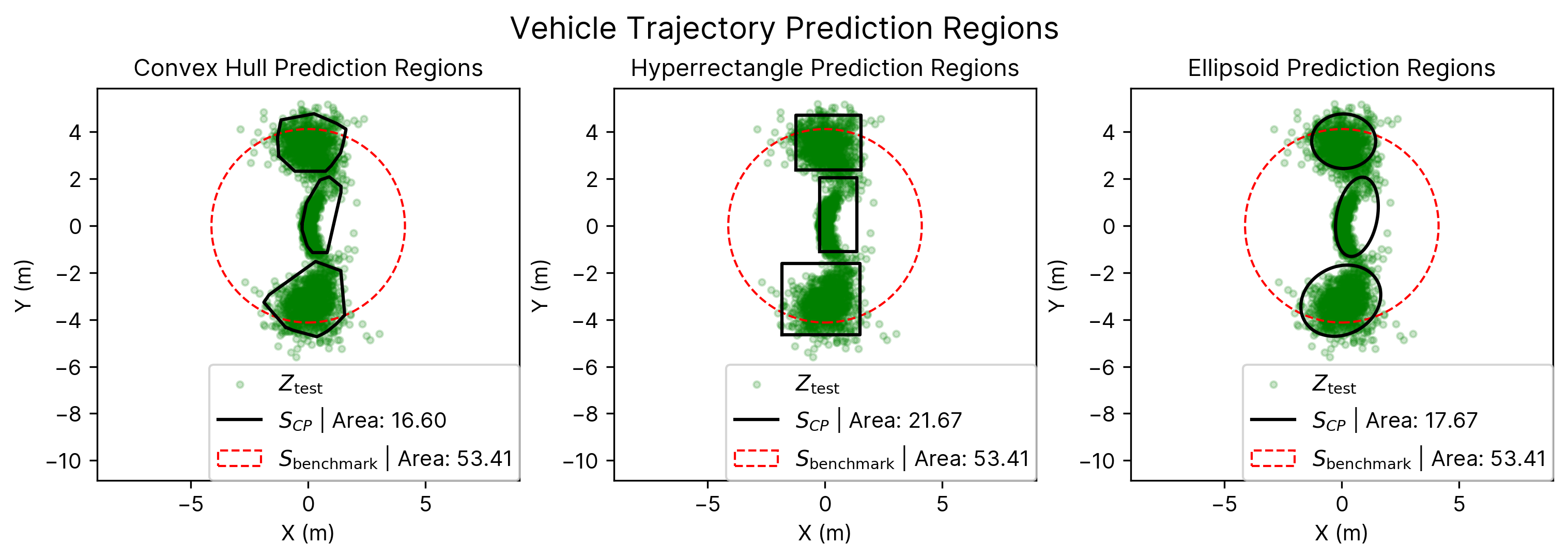
Figure 1: Vehicle Trajectory Prediction regions, $S_{CP}$, plotted alongside benchmark prediction regions $S_{\text{benchmark}}$, which are based on the 2-norm of the residual. All methods achieve the target $90\%$ coverage rate. The Convex Hull, Hyperrectangle, and Ellipsoid Regions are $68.92\%$, $59.43\%$, and $66.92\%$ smaller respectively.

Conformal prediction (CP) has emerged as a popular method for statistical uncertainty quantification [Shafer and Vovk(2008), Vovk et al.(2005)Vovk, Gammerman, and Shafer]. It aims to construct regions around a predictor’s output, called prediction regions, that contain the true but unknown quantity of interest with a user-defined probability. CP does not require any assumptions about the underlying distribution of the data or the predictor itself and instead one only needs a calibration dataset. This means that CP can be applied to learning-enabled predictors, such as neural networks [Angelopoulos et al.(2023)Angelopoulos, Bates, et al.].

Conformal prediction regions take the form $\{y|R(y,\hat{y})\leq C\}$, where $\hat{y}$ is a prediction and $R(y,\hat{y})\in\mathbb{R}$ is a non-conformity score function. This function quantifies the difference between the ground truth $y$ and the prediction $\hat{y}$, while $C\in\mathbb{R}$ is a bound produced by the CP procedure. The choice of non-conformity score function plays a vital role as it defines what shape and size the prediction regions take. For example, using the L2 norm on the error between $y$ and $\hat{y}$ ensures that the CP regions will be circles or hyperspheres depending on the dimension of $y$. However, if the distribution of errors from the predictor does not resemble a sphere, e.g., when there are dependencies across dimensions, then the L2 norm is not the right choice as it will result in unnecessarily large prediction regions. While there is initial work in this direction, see e.g., [Tumu et al.(2023)Tumu, Lindemann, Nghiem, and Mangharam] and [Cleaveland et al.(2023)Cleaveland, Lee, Pappas, and Lindemann], a systematic approach to generate non-conservative conformal prediction regions is missing.

Additionally, standard non-conformity score functions do not allow for disjoint prediction regions. This further leads to overly large prediction regions when prediction errors have multi-modal distributions, such as when predicting which way a vehicle will turn at an intersection, as shown by the dotted red circles in Figure 1. To address this issue, [Zecchin et al.(2023)Zecchin, Park, and Simeone] build prediction regions using multiple predictions. [Lei et al.(2011)Lei, Robins, and Wasserman, Smith et al.(2014)Smith, Nouretdinov, Craddock, Offer, and Gammerman] employ kernel density estimators (KDEs) which can capture disjoint prediction regions. However, KDE based prediction regions are mathematically difficult to handle and not suitable for real-time decision making. For example, [Lindemann et al.(2023a)Lindemann, Cleaveland, Shim, and Pappas, Dixit et al.(2023)Dixit, Lindemann, Wei, Cleaveland, Pappas, and Burdick] use conformal prediction regions for model predictive control which cannot handle prediction regions from KDEs efficiently. With this in mind, we also seek to produce conformal prediction regions that are practical. For our purposes, we generate prediction regions that are sets of either ellipsoids or convex polytopes. Another feature of our work is that we will optimize over template shapes under suitable optimality criteria.

Contributions. To address the conservatism from improper choices of non-conformity score functions, this paper proposes using optimization to create non-conformity score functions that produce non-conservative conformal prediction regions that are multi-modal and practical. Our main idea is to use an extra calibration dataset to i) cluster the residuals of this calibration data to identify different modes in the error distribution, ii) define parameterized shape generating functions which specify template shapes, iii) solve an optimization problem to fit parameterized shape functions for each cluster over the calibration data while minimizing the volume of the shape template, and iv) use the resulting set of shape template functions to define a non-conformity score function. Finally, we use a separate calibration dataset to apply CP using the new non-conformity score function. Our contributions are as follows:

• We propose a framework for generating non-conformity score functions that result in non-conservative conformal prediction regions that are multi-modal and practical. We capture multi-modality using clustering algorithms and obtain non-conservative convex regions by fitting parameterized shape template functions to each cluster.

• We provide a python toolbox of our method that can readily be used. We further demonstrate that our method produces non-conservative conformal prediction regions on case studies of F16 fighter jets and autonomous vehicles, showing an up to 68% reduction in prediction region area.

Related Work. The original conformal prediction approach, introduced by [Vovk et al.(2005)Vovk, Gammerman, and Shafer, Shafer and Vovk(2008)] to quantify uncertainty of prediction models, required training one prediction model per training datapoint, which is computationally intractable for complex predictors. To alleviate this issue, [Papadopoulos(2008)] introduce inductive conformal prediction, which can also be referred to as split conformal prediction. This method employs a calibration dataset for applying conformal prediction. Split conformal prediction has been extended to allow for quantile regression [Romano et al.(2019)Romano, Patterson, and Candes], to provide conditional statistical guarantees [Vovk(2012)], and to handle distribution shifts [Tibshirani et al.(2019)Tibshirani, Foygel Barber, Candes, and Ramdas, Fannjiang et al.(2022)Fannjiang, Bates, Angelopoulos, Listgarten, and Jordan]. Applications of split conformal prediction include out-of-distribution detection [Kaur et al.(2022a)Kaur, Jha, Roy, Park, Dobriban, Sokolsky, and Lee, Kaur et al.(2023)Kaur, Sridhar, Park, Yang, Jha, Roy, Sokolsky, and Lee], guaranteeing safety in autonomous systems [Luo et al.(2022)Luo, Zhao, Kuck, Ivanovic, Savarese, Schmerling, and Pavone], performing reachability analysis [Hashemi et al.(2023)Hashemi, Qin, Lindemann, and Deshmukh, Lindemann et al.(2023b)Lindemann, Qin, Deshmukh, and Pappas], and bounding errors in F1/10 car predictions [Tumu et al.(2023)Tumu, Lindemann, Nghiem, and Mangharam], while in [Stutz et al.(2022)Stutz, Dvijotham, Cemgil, and Doucet] the authors encode the width of the generated prediction sets directly into the loss function of a neural network during training. Additionally, prior works have constructed probably approximately correct prediction sets around conformal prediction regions [Park et al.(2020)Park, Bastani, Matni, and Lee, Angelopoulos et al.(2022)Angelopoulos, Bates, Fisch, Lei, and Schuster].

However, the aforementioned methods use either standard or handcrafted non-conformity score functions that may not fit the residuals of their predictors well, which could result in unnecessarily large prediction regions. Previous works have addressed this limitation by employing density estimators as non-conformity score functions. In [Lei et al.(2011)Lei, Robins, and Wasserman, Lei et al.(2013)Lei, Robins, and Wasserman, Lei and Wasserman(2014), Smith et al.(2014)Smith, Nouretdinov, Craddock, Offer, and Gammerman] the authors use kernel density estimators (KDEs) to produce conformal prediction regions. Another work uses conditional density estimators, which estimate the conditional distribution of the data $p(Y|X)$, to produce non-conformity scores [Izbicki et al.(2022)Izbicki, Shimizu, and Stern], while [Han et al.(2022)Han, Tang, Ghosh, and Liu] partitions the input space and employs KDEs over the partitions to compute density estimates, which allow for conditional coverage guarantees. While these approaches can produce small prediction regions, they may not have mathematical forms that are easy for downstream tasks to make use of. In a different vein, [Bai et al.(2022)Bai, Mei, Wang, Zhou, and Xiong] uses parameterized conformal prediction sets and expected risk minimization to produce small prediction regions.

Finally, some work has gone into producing multi-modal prediction regions. These works use set based predictors to compute multiple predictions and conformalize around these sets of predictions [Wang et al.(2023)Wang, Gao, Yin, Zhou, and Blei, Zecchin et al.(2023)Zecchin, Park, and Simeone, Parente et al.(2023)Parente, Darabi, Stutts, Tulabandhula, and Trivedi].

2 Preliminaries: Conformal Prediction Regions

Split Conformal Prediction. Conformal prediction was introduced in [Vovk et al.(2005)Vovk, Gammerman, and Shafer, Shafer and Vovk(2008)] to obtain valid prediction regions, e.g., for complex predictive models such as neural networks. Split conformal prediction is a computationally tractable variant of conformal prediction [Papadopoulos(2008)] where a calibration dataset is available that has not been used to train the predictor. Let $R_{0},R_{1}\ldots,R_{n}$ be $n+1$ exchangeable random variables, usually referred to as the nonconformity scores. Here, $R_{0}$ can be viewed as a test datapoint, and $R_{i}$ with $i\in\{1,\ldots,n\}$ as a set of calibration data. The nonconformity scores are often defined as $R:=\|Y-h(X)\|$ and $R_{i}:=\|Y_{i}-h(X_{i})\|$ where $h$ is a predictor that attempts to predict the output from the input. Our goal is now to obtain a probabilistic bound for $R_{0}$ based on $R_{1},\ldots,R_{n}$. Formally, given a failure probability $\delta\in(0,1)$, we want to compute a constant $C$ so that

$$\text{Prob}(R_{0}\leq C)\geq 1-\delta.$$ (1)

In conformal prediction, we compute $C:=\text{Quantile}(\{R_{1},\ldots,R_{n},\infty\},1-\delta)$ which is the $(1-\delta)$th quantile of the empirical distribution of the values $R_{1},\ldots,R_{n}$ and $\infty$. Alternatively, by assuming that $R_{1},\ldots,R_{n}$ are sorted in non-decreasing order and by adding $R_{n+1}:=\infty$, we can obtain $C=R_{p}$ where $p:=\lceil(n+1)(1-\delta)\rceil$ with $\lceil\cdot\rceil$ being the ceiling function, i.e., $C$ is the $p$th smallest nonconformity score. By a quantile argument, see [Tibshirani et al.(2019)Tibshirani, Foygel Barber, Candes, and Ramdas, Lemma 1], one can prove that this choice of $C$ satisfies  Equation 1. Note that $n\geq\lceil(n+1)(1-\delta)\rceil$ is required to hold to obtain meaningful, i.e., bounded, prediction regions.

Existing Choices for Non-Conformity Score Functions. The guarantees from (1) bound the non-conformity scores, and we need to convert this bound into prediction regions. Specifically, let $(X,Y)$ and $(X_{i},Y_{i})$ with $i\in\{1,\ldots,n\}$ be test and calibration data, respectively, drawn from a distribution $\mathcal{D}$, with $X,X_{i}\in\mathcal{X}\subseteq\mathbb{R}^{l}$ and $Y,Y_{i}\in\mathcal{Y}\subseteq\mathbb{R}^{p}$. Assume also that we are given a predictor $h:\mathcal{X}\rightarrow\mathcal{Y}$. First, we define a non-conformity score function $R$, which maps outputs and predicted outputs to the non-conformity scores from the previous section as $R:\mathcal{Y}\times\mathcal{Y}\rightarrow\mathbb{R}$.

Then, for a non-conformity score $R(Y,\hat{Y})$ with prediction $\hat{Y}:=h(X)$ and a constant $C$ that satisfies (1), e.g., obtained from calibration data $R(Y_{i},\hat{Y}_{i})$ with $\hat{Y}_{i}:=h(X_{i})$ using conformal prediction, we define the prediction region $S_{CP}$ as the set of values in $\mathcal{Y}$ that result in a non-conformity score not greater than $C$, i.e., such that

$$S_{CP}:=\{y\in\mathcal{Y}|R(y,\hat{Y})\leq C\}.$$ (2)

The choice of the score function $R$ greatly affects the shape and size of the prediction region $S_{CP}$. For example, if we use the L2 norm as $R(Y,\hat{Y}):=\|Y-\hat{Y}\|_{2}$, then the conformal prediction regions will be hyper-spheres (circles in two dimensions). However, the errors of the predictor $h$ may have asymmetric, e.g., more accurate in certain dimensions, and multi-modal distributions, which will result in unnecessarily conservative prediction regions. We are interested in constructing non-conservative and multi-modal prediction regions, e.g., as shown in Figure 1.

Often non-conformity score functions are fixed a-priori, e.g., as the aforementioned L2 norm distance [Lindemann et al.(2023a)Lindemann, Cleaveland, Shim, and Pappas] or by using softmax functions for classification tasks [Angelopoulos et al.(2023)Angelopoulos, Bates, et al.]. More tailored functions were presented in [Tumu et al.(2023)Tumu, Lindemann, Nghiem, and Mangharam] for F1/10 racing applications, in [Kaur et al.(2022b)Kaur, Sridhar, Park, Jha, Roy, Sokolsky, and Lee] for predictor equivariance, and in [Cleaveland et al.(2023)Cleaveland, Lee, Pappas, and Lindemann] for multi-step prediction regions of time series.

Data-driven techniques instead compute non-conformity scores from data. Existing techniques generally rely on density estimation techniques which aim to estimate the conditional distribution $p(Y|X)$ [Lei et al.(2011)Lei, Robins, and Wasserman]. Let $\hat{p}(Y|X)$ denote an estimate of $p(Y|X)$. One can then use the estimate $\hat{p}(Y|X)$ to define the non-conformity score as $R(Y,X):=-\hat{p}(Y|X)$. For this non-conformity score function, one can apply the conformal prediction to get a bound $C$ which results in the prediction region $S_{CP}=\{y|\hat{p}(y|X)\leq C\}$. These regions can take any shape and potentially be multi-modal. However, these regions are difficult to work with in downstream decision making tasks, especially if the model used to form $\hat{p}(Y|X)$ is complex (e.g. a deep neural network), as $\hat{p}$ needs to be inverted to obtain the region.

Problem Formulation. In this work, we present a combination of a data-driven technique with parameterized template non-conformity score functions. As a result, we obtain parameterized conformal prediction regions which we denote as $S_{CP,\theta}:=\{y\in\mathcal{Y}|R_{\theta}(y,\hat{Y})\leq C\}$ where $\theta$ is a set of parameters. Our high level problem is now to find values for $\theta$ that minimize the size of $S_{CP,\theta}$ while still achieving the desired coverage level $1-\delta$.

Problem 1

Let $(X,Y)\sim\mathcal{D}$ be a random variable, $D_{cal}:=\{(X_{1},Y_{1}),\ldots,(X_{n},Y_{n})\}$ be a calibration set of random variables independently drawn from $\mathcal{D}$, $h:\mathcal{X}\rightarrow\mathcal{Y}$ be a predictor, and $\delta\in(0,1)$ be a failure probability. Define parameterized template non-conformity score functions $R_{\theta}(Y,h(X))$ for parameters $\theta$ that result in convex multi-modal prediction regions $S_{CP,\theta}$, and use the calibration set $D_{cal}$ to solve the optimization problem:

$$\min_{\theta}\;\; \text{Volume}(S_{CP,\theta})$$ (3a)

s.t. $$\text{Prob}\left(Y\in S_{CP,\theta}\right)\geq 1-\delta$$ (3b)

We cannot exactly solve (3a), especially since one can run into trouble when using the same data to both compute the values of $\theta$ and compute the prediction region $S_{CP,\theta}$ based on $\theta$. So we aim to find heuristic solutions to (3a), with an added focus on having $S_{CP,\theta}$ be multi-modal and practical for downstream tasks.

3 Computing Convex Multi-Modal Conformal Prediction Regions

To enable multi-modal prediction regions, we first cluster the residuals $Y-\hat{Y}$ over a subset $D_{cal,1}$ of our calibration data $D_{cal}$, i.e., $D_{cal,1}\subset D_{cal}$. More specifically, we perform a density estimation step by using Kernel Density Estimation (KDE) to find high-density modes of residuals in $D_{cal,1}$. We then perform a clustering step by using Mean Shift Clustering to identify multi-modality in the high-density modes of the KDE. We next perform a shape construction step by defining parameterized shape template functions and by fitting a separate shape template function to each cluster. These shape template functions generate convex approximations of the identified clusters. We then perform a conformal prediction step where we combine all shape template functions into a single non-conformity score function. Finally, we apply conformal prediction to this non-conformity score over the calibration data $D_{cal,2}:=D_{cal}\setminus D_{cal,1}$. The use of a separate calibration set $D_{cal,2}$ guarantees the validity of our method. We explain each of these steps now in detail.

Density Estimation

Let us define the residuals $Z_{i}:=Y_{i}-\hat{Y}_{i}$ with $\hat{Y}_{i}:=h(X_{i})$ for each calibration point $(X_{i},Y_{i})\in D_{cal,1}$. We then define the set of residuals $Z:=\{Z_{1},\ldots,Z_{n_{1}}\}$ where $n_{1}:=|D_{cal,1}|$. We seek to understand the distribution of these residuals to build multi-modal prediction regions. For this purpose, we perform Kernel Density Estimation (KDE) over the residuals $Z$ of $D_{cal,1}$. In doing so, we will be able to capture high-density modes of the residual distribution.

KDE is an approach for estimating the probability density function of a variable from data [Parzen(1962), Rosenblatt(1956)]. The estimated density function using KDE takes the form

$$\hat{p}(z|\bar{K},b,Z_{1},\ldots,Z_{n_{1}})=\frac{1}{n_{1}b}\sum_{i=1}^{n_{1}}\bar{K}\left(\frac{z-Z_{i}}{b}\right)$$ (4)

where $Z_{1},\ldots,Z_{n_{1}}$ are the residuals from $D_{cal,1}$, $\bar{K}$ is a kernel function, and $b$ is the bandwidth parameter. The kernel $\bar{K}$ must be a non-negative, real-valued function. In this work, we use the Gaussian kernel $\bar{K}(z):=\frac{1}{\sqrt{2\pi}}\exp(-z^{2}/2)$, which is the density of the standard normal distribution. The bandwidth parameter $b$ controls how much the density estimates spread out from each residual $Z_{i}$, with larger values causing the density estimates to spread out less. We use Silverman’s rule of thumb [Silverman(1986)] to select the value of $b$. Using a combination of KDE with Silverman’s rule of thumb yields a parameter-free method of estimating the probability density of a given variable.

We use the KDE $\hat{p}$ to find a set $\bar{L}\subseteq\mathcal{Y}$ that covers a $1-\delta$ portion of the residuals, i.e., we want to compute $\bar{L}$ such that $1-\delta\leq\int_{\bar{L}}\hat{p}(z|\bar{K},b,Z_{1},\ldots,Z_{n_{1}})\,dz$. As $\bar{L}$ is difficult to compute in practice, our algorithm first grids the $Z$ domain. Let $J$ be the number of grid cells and let $g_{j}\subseteq\mathcal{Y}$ denote the $j$th grid cell. Next, we compute $\hat{p}(z_{j}^{c}|\bar{K},b,Z_{1},\ldots,Z_{n_{1}})$ for a single point $z_{j}^{c}\in g_{j}$ of each grid cell (e.g., its center) and multiply $\hat{p}(z_{j}^{c}|\bar{K},b,Z_{1},\ldots,Z_{n_{1}})$ by the volume of the grid cell to obtain its probability density. Finally, we sort the probability densities of all grid cells in decreasing order and add grid cells (start from high-density cells) to $\bar{L}$ until the cumulative sum of probability densities in $\bar{L}$ is greater than $1-\delta$. Having computed high density modes in $\bar{L}$, we construct the discrete set $L:=\{z_{1}^{c},\ldots,z_{J}^{c}\}$. We note that we will get valid prediction regions despite this discretization.

Clustering

In the next step, we identify clusters of points within $L$ toward obtaining multi-modal prediction regions. To accomplish this, we use the Mean Shift algorithm [Comaniciu and Meer(2002)] since it does not require a pre-specified number of clusters. The algorithm attempts to find local maxima of the probability density $\hat{p}$ within $L$. The algorithm requires a single bandwidth parameter, which we estimate from data using the bandwidth estimator package in [Pedregosa et al.(2011)Pedregosa, Varoquaux, Gramfort, Michel, Thirion, Grisel, Blondel, Prettenhofer, Weiss, Dubourg, Vanderplas, Passos, Cournapeau, Brucher, Perrot, and Duchesnay]. Due to space limitations, we direct the reader to [Comaniciu and Meer(2002)] for more details. Once the local maxima are found, we group all of the points within $L$ according to their nearest maxima, resulting in the set $L=:\{L_{1},\ldots,L_{K}\}$, where $K$ denotes the number of clusters.

Shape Construction

For each cluster $L_{k}\in L$, we now construct convex over-approximations. Our approximations are defined by parameterized shape template functions $f_{\theta_{k}}$ and take the form $S_{\theta_{k}}=\{z|f_{\theta_{k}}(z)\leq 0\}$. We specifically consider shape template functions for ellipsoid, convex hulls, and hyperrectangles (details are provided below). Given a cluster of points $L_{k}$ and a parameterized template function $f_{\theta_{k}}$, we find the parameters ${\theta_{k}}$ that minimize the volume of $S_{\theta_{k}}$ while covering all of the points in $L_{k}$. This is formulated as the following optimization problem:

$$\min_{\theta_{k}}\;\; \textrm{Volume}(S_{\theta_{k}})$$ (5a)

s.t. $$S_{\theta_{k}}=\{z|f_{\theta_{k}}(z)\leq 0\}$$ (5b)

$$z\in S_{\theta_{k}}\;\;\forall z\in L_{k}.$$ (5c)

After solving this optimization problem for each cluster $L_{k}\in L$, we get the set of shapes $S_{c}:=\{S_{\theta_{1}},\ldots,S_{\theta_{k}}\}$. Below, we provide our three choices of template shapes.

Ellipsoid: The definition for an ellipsoid in $\mathbb{R}^{p}$ parameterized by ${\theta_{k}}:=\{Q\succ 0\in\mathbb{R}^{p\times p},c\in\mathbb{R}^{p}\}$ is $\text{Ell}_{\theta_{k}}\coloneqq\{z\in\mathbb{R}^{p}|(z-c)^{T}Q(z-c)\leq 1\}$. The shape template function for an ellipsoid is

$$f_{\theta_{k}}(z):=(z-c)^{T}Q(z-c)-1.$$ (6)

We solve the problem in Equation 5 for $\theta_{k}$ (consisting of $Q$ and $c$) under this parameterization by using CMA-ES, a genetic algorithm [Hansen et al.(2003)Hansen, Müller, and Koumoutsakos, Hansen et al.(2023)Hansen, Yoshihikoueno, ARF1, Kadlecová, Nozawa, Rolshoven, Chan, Youhei Akimoto, Brieglhostis, and Brockhoff].

Convex Hull: The definition for a Convex Hull in $\mathbb{R}^{p}$ parameterized by ${\theta_{k}}:=\{A\in\mathbb{R}^{r\times p},b\in\mathbb{R}^{r}\}$ is $\textrm{CXH}_{\theta_{k}}:=\left\{z\in\mathbb{R}^{p}|Az-b\leq 0\right\}$, where $r$ is the number of facets in the Convex Hull. This way, the shape template function for a convex hull is

$$f_{\theta_{k}}(z):=\max_{j\in\{1,\ldots,r\}}A_{j}z-b_{j}$$ (7)

where $A_{j}$ and $b_{j}$ denote the $j^{th}$ row of $A$ and $b$, respectively. We solve the problem in Equation 5 for $\theta_{k}$ (consisting of $A$ and $b$) under this parameterization by using the Quickhull Algorithm from [Barber et al.(1996)Barber, Dobkin, and Huhdanpaa]. This algorithm generates a convex polytope that contains every point in $L_{k}$.

Hyper-Rectangle: The definition for a (non-rotated) hyper-rectangle parameterized by ${\theta_{k}}:=\{b_{min}\in\mathbb{R}^{p},b_{max}\in\mathbb{R}^{p}\}$ is $\textrm{HypRect}_{\theta_{k}}:=\left\{z\in\mathbb{R}^{p}|b_{min}\leq z\leq b_{max}\right\}$. Consequently, the shape template function for a hyper-rectangle is

$$f_{\theta_{k}}(z):=\max_{j\in\{1,\ldots,p\}}\max\left\{b_{min,j}-z_{j},z_{j}-b_{max,j}\right\}$$ (8)

We solve the problem in Equation 5 for $\theta_{k}$ (consisting of $b_{min}$ and $b_{max}$) under this parameterization by computing the element-wise minimum and maximum of the datapoints in $L_{k}$.

Conformalization

Note that the set $S_{c}=\{S_{\theta_{1}},\ldots,S_{\theta_{k}}\}$, while capturing information about the underlying distribution of residuals, may not be a valid prediction region. To obtain valid prediction regions, we define a new nonconformity score based on the shape template functions $\{f_{\theta_{1}},\ldots,f_{\theta_{k}}\}$ to which we then apply conformal prediction over the second dataset $D_{cal,2}$. To account for scaling differences in $f_{\theta_{k}}$, which each describe different regions, we normalize first. Specifically, we compute a normalization constant $\alpha_{k}$ for each $f_{\theta_{k}}$ as

$$\mathcal{R}_{k}:=\left\{f_{\theta_{k}}(z)\middle|z\in D_{cal,1}\right\}$$

$$\alpha_{k}:=1/\left(\text{Quantile}(\mathcal{R}_{k},1-\delta)-\min(\mathcal{R}_{k})\right)$$ (9)

We then define the non-conformity score for each shape as the normalized shape template function

$$R_{\theta_{k}}(z):=\alpha_{k}f_{\theta_{k}}(z).$$ (10)

Finally, we define the joint non-conformity score over all shapes using the smallest normalized non-conformity score as

$$R_{S_{c}}(z):=\text{min}(R_{\theta_{1}}(z),\ldots,R_{\theta_{K}}(z))$$ (11)

We remark here that we take the minimum because we only need the residual point $z$ to lie within one shape. We can then apply conformal prediction to this non-conformity score function over the second dataset $D_{cal,2}$ to obtain a valid multi-modal prediction region. The next result follows immediately by [Tibshirani et al.(2019)Tibshirani, Foygel Barber, Candes, and Ramdas, Lemma 1] and since we split $D_{cal}$ into $D_{cal,1}$ and $D_{cal,2}$.

Theorem 3.1.

Let the conditions from Problem 1 hold. Let $R_{S_{c}}$ be the non-conformity score function according to equation (11) where the parameters $\theta_{1},\ldots,\theta_{K}$ are obtained by solving Equation 5. Define $R:=R_{S_{c}}(Y-\hat{Y})$ for the random variable $(X,Y)\sim\mathcal{D}$ and $R_{i}:=R_{S_{c}}(Y_{i}-\hat{Y}_{i})$ for the calibration data $(X_{i},Y_{i})\in D_{cal,2}$ with $i\in\{n_{1}+1,\ldots,n\}$. Then, it holds that

$$Prob(R\leq C)\geq 1-\delta$$ (12)

where $C\coloneqq Quantile(\{R_{n_{1}+1},\ldots,R_{n},\infty\},1-\delta)$.

To convert the probabilistic guarantee in equation (12) into valid prediction regions, we note that

$$R=\text{min}(R_{\theta_{1}}(Z),\ldots,R_{\theta_{K}}(Z))\leq C\iff\exists k\in\{1,\ldots,K\}\;s.t.\;f_{\theta_{k}}(Z)\leq C/\alpha_{k}.$$ (13)

For a prediction $\hat{Y}$, this means in essence that a valid prediction region is defined by

$$S_{CP}:=\{y|\exists k\in\{1,\ldots,K\}\;s.t.\;f_{\theta_{k}}(y-\hat{Y})\leq C/\alpha_{k}\}=\cup_{k=1}^{K}\{y|f_{\theta_{k}}(y-\hat{Y})\leq C/\alpha_{k}\}$$ (14)

Intuitively, the conformal prediction region $S_{CP}$ is the union of the prediction regions around each shape in $S_{c}$ which illustrates its multi-modality. We summarize our results as a Corollary.

Corollary 3.2.

Let the conditions of Theorem 3.1 hold. Then, it holds that $\text{Prob}\left(Y\in S_{CP}\right)\geq 1-\delta$.

Dealing with Time-Series Data

Let us now illustrate how we can handle time series data. Assume that $S_{0},S_{1},\ldots,S_{T}\in\mathbb{R}^{p(T+1)}$ is a time series of length $T$ that follows the distribution $\mathcal{D}$. At time $t>0$, we observe the inputs $X:=(S_{0},\ldots,S_{t})$ and want to predict the outputs $Y:=(S_{t+1},\ldots,S_{T})$ with a trajectory predictor $h$, e.g., a recurrent neural network. Our calibration dataset $D_{cal,1}$ consists of pairs $(X,Y)\sim\mathcal{D}$ where $X=(S_{0},\ldots,S_{t})$ and $Y=(S_{t+1},\ldots,S_{T})$ and the residuals are $Z_{\tau}=S_{\tau}-h(X)_{\tau}$ for $\tau=t+1,\ldots,T$. Now, our desired prediction region should contain every future value of the time series, $S_{t+1},\ldots,S_{T}$, with probability $1-\delta$. To achieve this in a computationally efficient manner, we follow the previously proposed optimization procedure for each future time $\tau\in\{t+1,\ldots,T\}$ independently again with a desired coverage of $1-\delta$. As a result, we get a non-conformity score $R_{S_{c}}^{\tau}$ for each time $\tau$, similarly to Equation 11. We normalize these scores over the future times, obtaining normalization constants $\beta_{\tau}$, as in Equation 15. Finally, we need to compute the joint non-conformity score over all future times as in Equation 16.

$$\bar{\mathcal{R}}_{\tau}:=\left\{R_{S_{c}}^{\tau}(Z_{\tau})\middle|Z_{\tau}\in D_{cal,1}\right\}$$

$$\beta_{\tau}:=1/\left(\text{Quantile}(\bar{\mathcal{R}}_{\tau},1-\delta)-\min(\bar{\mathcal{R}}_{\tau})\right)$$ (15)

$$R_{S_{c}}(Z):=\max_{\tau\in\{t+1,\ldots,T\}}\beta_{\tau}R_{S_{c}}^{\tau}(Z_{\tau})$$ (16)

Note here that we take the maximum, as inspired by our prior work [Cleaveland et al.(2023)Cleaveland, Lee, Pappas, and Lindemann], to obtain valid coverage over all future times. We can now apply conformal prediction to $R_{S_{c}}$ in the same way as in Theorem 3.1 to obtain valid prediction regions for time series.

4 Simulations

The toolbox and all experiments below are available on Github. To evaluate our approaches, we perform case studies on simulations of an F16 fighter jet performing ground avoidance maneuvers and a vehicle trajectory prediction scenario. Our method can be applied to our examples in two simple function calls after initialization.

⬇

pcr = ConformityOptimizer(”kde”, ”meanshift”, ”convexhull”, 0.90)

pcr.fit(Z_cal_one)

pcr.conformalize(Z_cal_two)

4.1 F16

In this case study, we analyze an F16 fighter jet performing ground avoidance maneuvers using the open source simulator from [Heidlauf et al.(2018)Heidlauf, Collins, Bolender, and Bak]. We use an LSTM to predict the altitude and pitch angle of the F16 up to $2.5$ seconds into the future at a rate of $10$ Hz ($25$ predictions in total) with the altitude and pitch from the previous $2.5$ seconds as input. The LSTM architecture consists of two layers of width $25$ and a final linear layer. We used $1500$ trajectories to train the network.

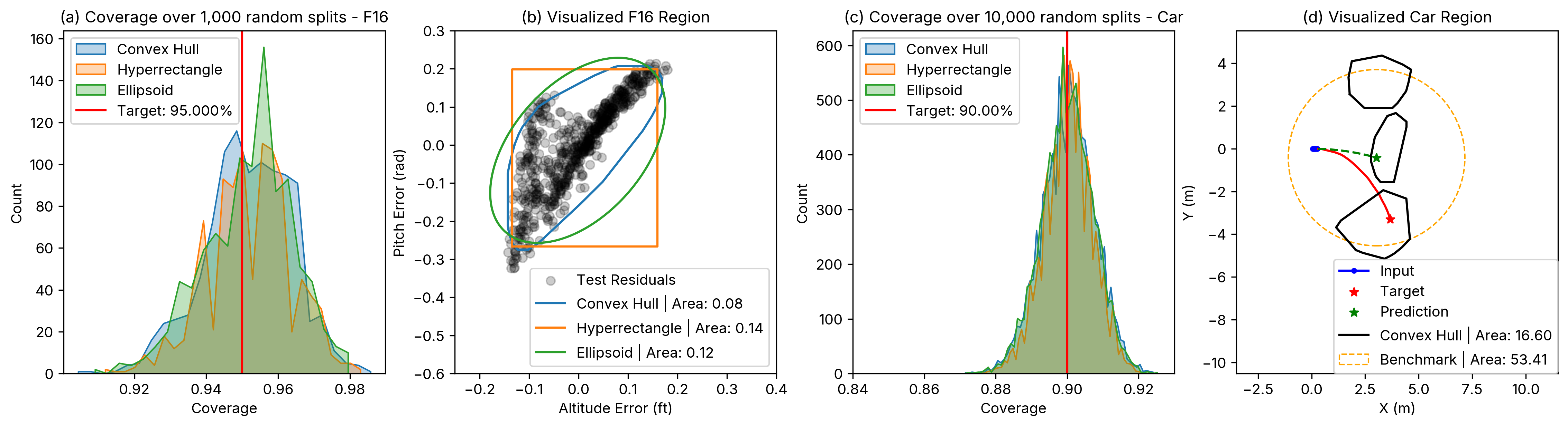
Figure 2: (a) Shows the coverage rates over 1,000 random splits of $D_{cal,2}$ and $D_{val}$ for the F16 example. (b) Shows fit conformal regions for the F16 example. (c) Shows the coverage rates over 10,000 random splits of $D_{cal,2}$ and $D_{val}$ for the car example. (d) Shows an example of the prediction regions shown on an actual prediction of the trajectories.

For calibration and validation, we collect a dataset of 1,900 trajectories all with length $5$ seconds. We randomly select 627 trajectories for $D_{cal,1}$, 627 for $D_{cal,2}$, and 646 for $D_{val}$. To account for the spread of the data, the bandwidth estimate was adjusted by a factor of $0.2$. Shapes were fit using the procedure described above, using a target coverage of $1-\delta=0.9$. The density estimation took $0.2949\text{s}$ on average and the clustering took $7.4222\text{s}$ on average. The average shape fitting times were $1.19\text{s}$ for the ellipse, $0.0030\text{s}$ for the convex hull, and $0.00086\text{s}$ for the hyperrectangle. Plots of the computed regions are shown in Figure 2(b) and coverage over 1000 random splits of $D_{cal,2}$ and $D_{val}$ are shown in Figure 2(a). The L2 norm benchmark region has a volume of $0.205$. Our regions provide a $31.7-60.9\%$ decrease in the area of the region, depending on the shape template used. In this example, differing units in each dimension are better compensated for in our approach.

4.2 Vehicle Trajectory Prediction

In this example application, we apply our method to the prediction of a vehicle’s trajectory. The vehicle is governed according to kinematic dynamics, which are given by Equation 17. The vehicle state contains its 2D position $x,y$, yaw $\theta$, and velocity $v$. The control inputs are the acceleration $a$ and steering angle $\omega$. For simplicity, we assume no acceleration commands (so $a=0$).

$$\dot{x}=v\cos(\theta),\quad\dot{y}=v\sin(\theta),\quad\dot{\theta}=v\tan(\omega)/L,\quad\dot{v}=a;\quad s=[x,y,\theta,v],\quad u=[\omega,a]$$ (17)

We use a physics-based, Constant Turn Rate and Velocity (CTRV) method to predict the trajectories of the car. The predictor takes as input the previous $0.5$ seconds of the state of the car (sampled at $10$Hz). It then estimates $\dot{\theta}$ by computing the average rate of change of $\theta$ over the inputs. It then uses this estimate along with the current state of the car to predict the future position of the car up to $5$ seconds into the future at a rate of $10$Hz ($50$ predictions total) using (17).

The predictor is evaluated on a scenario which represents an intersection. The vehicle proceeds straight for $0.5$ seconds, then either proceeds forward, turns left, or turns right for $5$ seconds, all with equal probability. The predictor makes its predictions at the end of the $0.5$ straight period. We generated $10000$ samples from this scenario. Of these, $3333$ samples were placed in $D_{cal,1}$, $3333$ in $D_{cal,2}$, and $3334$ in the test set.

First, we fit shapes for just the last timestep of the scenario, $5$ seconds into the prediction window, using the procedure described above with a target coverage of $1-\delta=0.9$. To account for the spread of the data, the bandwidth estimation was adjusted by a factor of $0.2$. We evaluated our approach on $10000$ random splits of the data in $D_{cal,1}$ and $D_{test}$. Computing the density estimate took $0.832\text{s}$ on average and the clusters took $0.856\text{s}$ on average. Fitting the shape templates took an average of $0.002\text{s}$ for the Convex Hull and Hyperrectangle and $3.760\text{s}$ for the Ellipse. The online portion, evaluating region membership, took $0.0029\text{s}$ on average for $3334$ points for all shapes. For each of the shape templates, we show that the mean coverage is close to our target coverage of $90\%$ in Figure 2(c). The figure is shown in Figure 2(d), and can be compared to the baseline circular region. Our method provides a $68.9\%$ improvement in the prediction region area while still providing the desired coverage. This figure also showcases the multi-modal capabilities of our approach, where each of the three behaviors has its own shape.

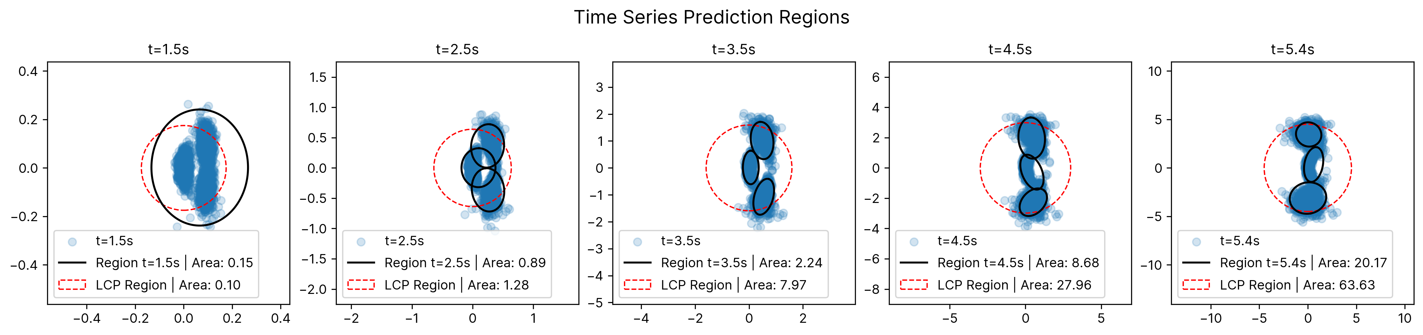
Figure 3: This figure shows the size of conformal prediction regions created for a time series prediction of vehicle motion over fifty timesteps. We generate a prediction region for only the timesteps shown, using the method in [Cleaveland et al.(2023)Cleaveland, Lee, Pappas, and Lindemann], labeled the LCP region. We also generate conformal prediction regions using our method, which are shown in black. Each figure includes the area of the regions shown, and all methods achieve the desired coverage.

Finally, we computed regions over multiple timesteps. Figure 3 shows the size and shape of the regions designed to achieve $90\%$ coverage over 5 timesteps. This prediction region takes $28\text{s}$ to compute, and $0.008\text{s}$ to compute region membership. The total volume of the prediction region is $68.17\%$ smaller than the benchmark approach from [Cleaveland et al.(2023)Cleaveland, Lee, Pappas, and Lindemann].

5 Conclusion

In this paper, we have presented a method for generating practical, multi-modal conformal prediction regions. Our approach uses an extra calibration dataset to find parameters of shape template functions over clusters of the calibration data. These shape template functions then get converted into a non-conformity score function, which we can use alongside standard inductive conformal prediction to get valid prediction regions. We demonstrate the approach on case studies of F16 fighter jets and autonomous vehicles, showing an up to 68% reduction in prediction region area.

References

- [Angelopoulos et al.(2022)Angelopoulos, Bates, Fisch, Lei, and Schuster] Anastasios N Angelopoulos, Stephen Bates, Adam Fisch, Lihua Lei, and Tal Schuster. Conformal risk control. arXiv preprint arXiv:2208.02814, 2022.
- [Angelopoulos et al.(2023)Angelopoulos, Bates, et al.] Anastasios N Angelopoulos, Stephen Bates, et al. Conformal prediction: A gentle introduction. Foundations and Trends® in Machine Learning, 16(4):494–591, 2023.
- [Bai et al.(2022)Bai, Mei, Wang, Zhou, and Xiong] Yu Bai, Song Mei, Huan Wang, Yingbo Zhou, and Caiming Xiong. Efficient and differentiable conformal prediction with general function classes. arXiv preprint arXiv:2202.11091, 2022.
- [Barber et al.(1996)Barber, Dobkin, and Huhdanpaa] C. Bradford Barber, David P. Dobkin, and Hannu Huhdanpaa. The quickhull algorithm for convex hulls. ACM Transactions on Mathematical Software, 22(4):469–483, December 1996. ISSN 0098-3500. 10.1145/235815.235821.
- [Cleaveland et al.(2023)Cleaveland, Lee, Pappas, and Lindemann] Matthew Cleaveland, Insup Lee, George J Pappas, and Lars Lindemann. Conformal prediction regions for time series using linear complementarity programming. arXiv preprint arXiv:2304.01075, 2023.
- [Comaniciu and Meer(2002)] D. Comaniciu and P. Meer. Mean shift: a robust approach toward feature space analysis. IEEE Transactions on Pattern Analysis and Machine Intelligence, 24(5):603–619, May 2002. ISSN 1939-3539. 10.1109/34.1000236. Conference Name: IEEE Transactions on Pattern Analysis and Machine Intelligence.
- [Dixit et al.(2023)Dixit, Lindemann, Wei, Cleaveland, Pappas, and Burdick] Anushri Dixit, Lars Lindemann, Skylar X Wei, Matthew Cleaveland, George J Pappas, and Joel W Burdick. Adaptive conformal prediction for motion planning among dynamic agents. In Learning for Dynamics and Control Conference, pages 300–314. PMLR, 2023.
- [Fannjiang et al.(2022)Fannjiang, Bates, Angelopoulos, Listgarten, and Jordan] Clara Fannjiang, Stephen Bates, Anastasios N Angelopoulos, Jennifer Listgarten, and Michael I Jordan. Conformal prediction under feedback covariate shift for biomolecular design. Proceedings of the National Academy of Sciences, 119(43):e2204569119, 2022.
- [Han et al.(2022)Han, Tang, Ghosh, and Liu] Xing Han, Ziyang Tang, Joydeep Ghosh, and Qiang Liu. Split localized conformal prediction. arXiv preprint arXiv:2206.13092, 2022.
- [Hansen et al.(2003)Hansen, Müller, and Koumoutsakos] Nikolaus Hansen, Sibylle D. Müller, and Petros Koumoutsakos. Reducing the Time Complexity of the Derandomized Evolution Strategy with Covariance Matrix Adaptation (CMA-ES). Evolutionary Computation, 11(1):1–18, March 2003. ISSN 1063-6560. 10.1162/106365603321828970.
- [Hansen et al.(2023)Hansen, Yoshihikoueno, ARF1, Kadlecová, Nozawa, Rolshoven, Chan, Youhei Akimoto, Brieglhostis, and Brockhoff] Nikolaus Hansen, Yoshihikoueno, ARF1, Gabriela Kadlecová, Kento Nozawa, Luca Rolshoven, Matthew Chan, Youhei Akimoto, Brieglhostis, and Dimo Brockhoff. CMA-ES/pycma: r3.3.0, January 2023.
- [Hashemi et al.(2023)Hashemi, Qin, Lindemann, and Deshmukh] Navid Hashemi, Xin Qin, Lars Lindemann, and Jyotirmoy V Deshmukh. Data-driven reachability analysis of stochastic dynamical systems with conformal inference. arXiv preprint arXiv:2309.09187, 2023.
- [Heidlauf et al.(2018)Heidlauf, Collins, Bolender, and Bak] Peter Heidlauf, Alexander Collins, Michael Bolender, and Stanley Bak. Reliable prediction intervals with directly optimized inductive conformal regression for deep learning. 5th International Workshop on Applied Verification for Continuous and Hybrid Systems (ARCH 2018), 2018.
- [Izbicki et al.(2022)Izbicki, Shimizu, and Stern] Rafael Izbicki, Gilson Shimizu, and Rafael B. Stern. Cd-split and hpd-split: Efficient conformal regions in high dimensions. J. Mach. Learn. Res., 23(1), jan 2022. ISSN 1532-4435.
- [Kaur et al.(2022a)Kaur, Jha, Roy, Park, Dobriban, Sokolsky, and Lee] Ramneet Kaur, Susmit Jha, Anirban Roy, Sangdon Park, Edgar Dobriban, Oleg Sokolsky, and Insup Lee. idecode: In-distribution equivariance for conformal out-of-distribution detection. Proceedings of the AAAI Conference on Artificial Intelligence, 36(7):7104–7114, Jun. 2022a. 10.1609/aaai.v36i7.20670.
- [Kaur et al.(2022b)Kaur, Sridhar, Park, Jha, Roy, Sokolsky, and Lee] Ramneet Kaur, Kaustubh Sridhar, Sangdon Park, Susmit Jha, Anirban Roy, Oleg Sokolsky, and Insup Lee. Codit: Conformal out-of-distribution detection in time-series data. arXiv preprint arXiv:2207.11769, 2022b.
- [Kaur et al.(2023)Kaur, Sridhar, Park, Yang, Jha, Roy, Sokolsky, and Lee] Ramneet Kaur, Kaustubh Sridhar, Sangdon Park, Yahan Yang, Susmit Jha, Anirban Roy, Oleg Sokolsky, and Insup Lee. Codit: Conformal out-of-distribution detection in time-series data for cyber-physical systems. In Proceedings of the ACM/IEEE 14th International Conference on Cyber-Physical Systems (with CPS-IoT Week 2023), pages 120–131, 2023.
- [Lei and Wasserman(2014)] Jing Lei and Larry Wasserman. Distribution-free prediction bands for non-parametric regression. Journal of the Royal Statistical Society Series B: Statistical Methodology, 76(1):71–96, 2014.
- [Lei et al.(2011)Lei, Robins, and Wasserman] Jing Lei, James Robins, and Larry Wasserman. Efficient nonparametric conformal prediction regions. arXiv preprint arXiv:1111.1418, 2011.
- [Lei et al.(2013)Lei, Robins, and Wasserman] Jing Lei, James Robins, and Larry Wasserman. Distribution-free prediction sets. Journal of the American Statistical Association, 108(501):278–287, 2013.
- [Lindemann et al.(2023a)Lindemann, Cleaveland, Shim, and Pappas] Lars Lindemann, Matthew Cleaveland, Gihyun Shim, and George J. Pappas. Safe planning in dynamic environments using conformal prediction. IEEE Robotics and Automation Letters, 8(8):5116–5123, 2023a. 10.1109/LRA.2023.3292071.
- [Lindemann et al.(2023b)Lindemann, Qin, Deshmukh, and Pappas] Lars Lindemann, Xin Qin, Jyotirmoy V. Deshmukh, and George J. Pappas. Conformal prediction for stl runtime verification. In Proceedings of the ACM/IEEE 14th International Conference on Cyber-Physical Systems (with CPS-IoT Week 2023), ICCPS ’23, page 142–153, 2023b. ISBN 9798400700361. 10.1145/3576841.3585927.
- [Luo et al.(2022)Luo, Zhao, Kuck, Ivanovic, Savarese, Schmerling, and Pavone] Rachel Luo, Shengjia Zhao, Jonathan Kuck, Boris Ivanovic, Silvio Savarese, Edward Schmerling, and Marco Pavone. Sample-efficient safety assurances using conformal prediction. In Algorithmic Foundations of Robotics XV: Proceedings of the Fifteenth Workshop on the Algorithmic Foundations of Robotics, pages 149–169. Springer, 2022.
- [Papadopoulos(2008)] Harris Papadopoulos. Inductive conformal prediction: Theory and application to neural networks. In Tools in artificial intelligence. Citeseer, 2008.
- [Parente et al.(2023)Parente, Darabi, Stutts, Tulabandhula, and Trivedi] Domenico Parente, Nastaran Darabi, Alex C Stutts, Theja Tulabandhula, and Amit Ranjan Trivedi. Conformalized multimodal uncertainty regression and reasoning. arXiv preprint arXiv:2309.11018, 2023.
- [Park et al.(2020)Park, Bastani, Matni, and Lee] Sangdon Park, Osbert Bastani, Nikolai Matni, and Insup Lee. Pac confidence sets for deep neural networks via calibrated prediction. In International Conference on Learning Representations, 2020.
- [Parzen(1962)] Emanuel Parzen. On Estimation of a Probability Density Function and Mode. The Annals of Mathematical Statistics, 33(3):1065–1076, 1962. ISSN 0003-4851. Publisher: Institute of Mathematical Statistics.
- [Pedregosa et al.(2011)Pedregosa, Varoquaux, Gramfort, Michel, Thirion, Grisel, Blondel, Prettenhofer, Weiss, Dubourg, Vanderplas, Passos, Cournapeau, Brucher, Perrot, and Duchesnay] F. Pedregosa, G. Varoquaux, A. Gramfort, V. Michel, B. Thirion, O. Grisel, M. Blondel, P. Prettenhofer, R. Weiss, V. Dubourg, J. Vanderplas, A. Passos, D. Cournapeau, M. Brucher, M. Perrot, and E. Duchesnay. Scikit-learn: Machine learning in Python. Journal of Machine Learning Research, 12:2825–2830, 2011.
- [Romano et al.(2019)Romano, Patterson, and Candes] Yaniv Romano, Evan Patterson, and Emmanuel Candes. Conformalized quantile regression. Advances in neural information processing systems, 32, 2019.
- [Rosenblatt(1956)] Murray Rosenblatt. Remarks on Some Nonparametric Estimates of a Density Function. The Annals of Mathematical Statistics, 27(3):832–837, September 1956. ISSN 0003-4851, 2168-8990. 10.1214/aoms/1177728190. Publisher: Institute of Mathematical Statistics.
- [Shafer and Vovk(2008)] Glenn Shafer and Vladimir Vovk. A tutorial on conformal prediction. Journal of Machine Learning Research, 9(3), 2008.
- [Silverman(1986)] Bernard W. Silverman. Density Estimation for Statistics and Data Analysis. CRC Press, April 1986. ISBN 978-0-412-24620-3.
- [Smith et al.(2014)Smith, Nouretdinov, Craddock, Offer, and Gammerman] James Smith, Ilia Nouretdinov, Rachel Craddock, Charles Offer, and Alexander Gammerman. Anomaly detection of trajectories with kernel density estimation by conformal prediction. In Lazaros Iliadis, Ilias Maglogiannis, Harris Papadopoulos, Spyros Sioutas, and Christos Makris, editors, Artificial Intelligence Applications and Innovations, pages 271–280, Berlin, Heidelberg, 2014. Springer Berlin Heidelberg.
- [Stutz et al.(2022)Stutz, Dvijotham, Cemgil, and Doucet] David Stutz, Krishnamurthy Dj Dvijotham, Ali Taylan Cemgil, and Arnaud Doucet. Learning optimal conformal classifiers. In International Conference on Learning Representations, 2022.
- [Tibshirani et al.(2019)Tibshirani, Foygel Barber, Candes, and Ramdas] Ryan J Tibshirani, Rina Foygel Barber, Emmanuel Candes, and Aaditya Ramdas. Conformal prediction under covariate shift. Advances in neural information processing systems, 32, 2019.
- [Tumu et al.(2023)Tumu, Lindemann, Nghiem, and Mangharam] Renukanandan Tumu, Lars Lindemann, Truong Nghiem, and Rahul Mangharam. Physics Constrained Motion Prediction with Uncertainty Quantification. In 2023 IEEE Intelligent Vehicles Symposium (IV), pages 1–8, Anchorage, AK, USA, June 2023. IEEE. 10.1109/IV55152.2023.10186812.
- [Vovk(2012)] Vladimir Vovk. Conditional validity of inductive conformal predictors. In Asian conference on machine learning, pages 475–490. PMLR, 2012.
- [Vovk et al.(2005)Vovk, Gammerman, and Shafer] Vladimir Vovk, Alexander Gammerman, and Glenn Shafer. Algorithmic learning in a random world. Springer Science & Business Media, 2005.
- [Wang et al.(2023)Wang, Gao, Yin, Zhou, and Blei] Zhendong Wang, Ruijiang Gao, Mingzhang Yin, Mingyuan Zhou, and David Blei. Probabilistic conformal prediction using conditional random samples. In Proceedings of The 26th International Conference on Artificial Intelligence and Statistics, pages 8814–8836, 25–27 Apr 2023.
- [Zecchin et al.(2023)Zecchin, Park, and Simeone] Matteo Zecchin, Sangwoo Park, and Osvaldo Simeone. Forking uncertainties: Reliable prediction and model predictive control with sequence models via conformal risk control. arXiv preprint arXiv:2310.10299, 2023.