Schwarzschild black hole and redshift rapidity:
A new approach towards measuring cosmic distances

Abstract

Motivated by recent achievements of a full general relativistic method in estimating the mass-to-distance ratio of supermassive black holes hosted at the core of active galactic nuclei, we introduce the new concept redshift rapidity in order to express the Schwarzschild black hole mass and its distance from the Earth just in terms of observational quantities. The redshift rapidity is also an observable relativistic invariant that represents the evolution of the frequency shift with respect to proper time in the Schwarzschild spacetime. We extract concise and elegant analytic formulas that allow us to disentangle mass and distance to black holes in the Schwarzschild background and estimate these parameters separately. This procedure is performed in a completely general relativistic way with the aim of improving the precision in measuring cosmic distances to astrophysical compact objects. Our exact formulas are valid on the midline and close to the line of sight, having direct astrophysical applications for megamaser systems, whereas the general relations can be employed in black hole parameter estimation studies.

Keywords: Schwarzschild black hole, black hole rotation curves, redshift and blueshift, redshift rapidity.

I Introduction

Black holes first have been found just as mathematical solutions to Einstein field equations of the general relativity theory by Karl Schwarzschild whereas their existence in the cosmos has been recently approved through gravitational wave detections GW  and electromagnetic wave observations EHTM87 ; EHTSgr . However, investigating the motion of stars around the center of our galaxy has already provided convincing evidence for the presence of a supermassive black hole hosted at the core of the Milky Way galaxy Ghez ; Morris ; Eckart ; Gillessen .

Even though the aforementioned methods are fairly accurate in obtaining the black hole parameters, they are not always applicable to existing data from black holes and black hole environments. Therefore, we have been inventing and developing an independent general relativistic approach to measure the black hole and cosmological parameters PRDhn ; PRDbhmn ; KdS . This method is based on the observational frequency-shifted photons emitted by massive geodesic particles orbiting central black holes and has been initially suggested in PRDhn , generalizing previous Keplerian models Herrnstein2005 ; Argon2007 ; Humphreys2013 . Recently, this approach has been developed to analytically express the mass and spin parameters of the Kerr black hole in terms of a few directly observational quantities PRDbhmn . Besides, it has been demonstrated that the Kerr black hole in asymptotically de Sitter background allows us to measure the Hubble constant and black hole parameters, simultaneously KdS .

The initial method of PRDhn  has been employed to obtain the kinematic redshift and blueshift in terms of black hole parameters for several black hole solutions, such as Kerr-Newman black holes in de Sitter spacetime KNdS , the Plebanski-Demianski black holes PlebanskiDemianski , higher dimensional Myers-Perry spacetime MyersPerry , and regular black holes in nonlinear electrodynamics RegularBH . Furthermore, a similar relation for the kinematic redshift has been found for black holes in modified gravity MOG , black holes coupled to nonlinear electrodynamics NED , black holes immersed in a strong magnetic field SMF , and the boson stars BosonStar .

These studies have been performed based on the kinematic frequency shift which is not an observable quantity, unlike the total frequency shift of photons. Hence, this fact has motivated us to consider the total frequency shift as a directly observable element and extract concise and elegant analytic formulas for the mass and spin of the Kerr black hole in terms of few observable quantities PRDbhmn . With the help of this general relativistic method, the free parameters of polymerized black holes have been expressed in terms of the total redshift as well FuZhang . More recently, this approach has been extended to general spherically symmetric spacetimes in order to extract the information of free parameters of black holes in alternative gravitational theories beyond Einstein gravity Diego .

From a practical point of view, the mass-to-distance ratio of several supermassive black holes hosted at the core of the active galactic nuclei (AGNs) NGC 4258 ApJL , TXS-2226-184 TXS , and an additional $15$ galaxies TenAGNs ; FiveAGNs has been estimated by employing this general relativistic approach. These supermassive black holes enjoy circularly orbiting water vapor clouds within accretion disks that emit redshifted photons toward a distant observer. This allows us to utilize the general relativistic method in order to estimate the $M/D$ ratio and quantify the gravitational redshift produced by the spacetime curvature which is a general relativistic effect.

In the parameter estimation studies of the supermassive black holes performed in ApJL ; TXS ; TenAGNs ; FiveAGNs , just the mass-to-distance ratio $M/D$ of these compact objects has been estimated with the help of observational redshifted and blueshifted photons due to the fact that this ratio is degenerate in this general relativistic formalism. In this paper, we are going to introduce a new general relativistic invariant observable quantity, the redshift rapidity, which is the derivative of the redshift with respect to proper time. With the aid of the redshift rapidity, we shall disentangle $M$ and $D$ in the Schwarzschild background to extract concise and elegant analytic formulas for mass and distance to the black hole just in terms of observational elements. Thus, these formulas will help us to break the degeneracy in the $M/D$ ratio of the Schwarzschild black hole and compute the mass and distance to the black hole separately. We would like to remark that these new formulas enable us to compute the distance to black holes and other astrophysical compact objects in a completely general relativistic framework with the aim of improving the precision in measuring cosmic distances with respect to previous Keplerian approaches that compute the angular-diameter distance to several megamaser galaxies like UGC 3789 MCP2 , NGC 6264 MCPV , NGC 5765b MCPVIII , NGC 4258 Humphreys2013 ; Reid2019 , CGCG 074-064 MCPXI , among others.

The outline of this paper is as follows. The next section is devoted to a brief review of our general relativistic formalism in the Schwarzschild black hole spacetime. Then, we express the mass-to-distance ratio of the Schwarzschild black hole in terms of observable frequency shifts for three spacial points of the circular motion of orbiting massive particles, namely, on the midline and close to the line of sight. In Sec. III, we define redshift rapidity as the proper time evolution of the frequency shift in the Schwarzschild background and employ this observable quantity in order to express the black hole mass and distance just in terms of observational elements on the midline and close to the line of sight. We finish our paper with some concluding remarks.

II Schwarzschild black hole and the frequency shift

In order to describe our formalism to measure cosmic distances, we start with a brief review on frequency shift formulas of massive probe particles in the Schwarzschild background based on PRDbhmn . The Schwarzschild black hole metric is given by the following line element

$$ds^{2}=g_{tt}dt^{2}+g_{rr}dr^{2}+g_{\theta\theta}d\theta^{2}+g_{\varphi\varphi}d\varphi^{2},$$ (1)

with the metric components

$$g_{\mu\nu}=diag\left[-\left(1-\frac{2M}{r}\right),\left(1-\frac{2M}{r}\right)^{-1},r^{2},r^{2}\sin^{2}\theta\right],$$ (2)

where $M$ is the total mass of the black hole and the event horizon is located at the Schwarzschild radius $r_{+}=2M$.

The massive geodesic particles revolving the Schwarzschild black hole feel the curvature of spacetime produced by the black hole mass and keep memory of it. Besides, the observers located on these particles can exchange redshifted photons that have information about the Schwarzschild black hole mass in their frequency from emission till detection. Thus, the shifts in the frequency of photons along with the orbital parameters of the emitter can be used to determine the black hole parameters ApJL ; TXS ; TenAGNs ; FiveAGNs . Therefore, this formalism allows one to compute the black hole parameters in terms of directly measured observational quantities and the orbital parameter of the emitter PRDbhmn ; FuZhang ; Diego .

Within General Relativity, the frequency of a photon that is emitted/detected by an emitter/observer with the proper $4$-velocity $U_{p}^{\mu}=(U^{t},U^{r},U^{\theta},U^{\varphi})\mid_{p}$ at some position $x_{p}^{\mu}=(x^{t},x^{r},x^{\theta},x^{\varphi})\mid_{p}$ reads

$$\omega_{p}=-\left(k_{\mu}U^{\mu}\right)\mid_{p}\,,$$ (3)

where $k_{p}^{\mu}=\left(k^{t},k^{r},k^{\theta},k^{\varphi}\right)\mid_{p}$ is the $4$-momentum of the photons with the null condition $k_{\mu}k^{\mu}=0$ and the index _p refers to either the emission point $x_{e}^{\mu}$ or detection point $x_{d}^{\mu}$ of the photons. Additionally, the $4$-velocity of particles is normalized to unity $U_{\mu}U^{\mu}=-1$, and when the detector’s orbit is located far away from the emitter-black hole system, $U_{d}^{\mu}$ reduces to

$$U_{d}^{\mu}=(1,0,0,0)\,.$$ (4)

The frequency shift of light signals emitted by massive geodesic particles in equatorial circular orbits revolving the spherically symmetric background (1) is given by PRDhn ; PRDbhmn

$$1+z_{{}_{Schw}}\!=\frac{\omega_{e}}{\omega_{d}}=\frac{(E_{\gamma}U^{t}-L_{\gamma}U^{\varphi})\mid_{e}}{(E_{\gamma}U^{t}-L_{\gamma}U^{\varphi})\mid_{d}},$$ (5)

where the conserved quantities $E_{\gamma}$ and $L_{\gamma}$ stand for the total energy and axial angular momentum of the photons. By considering Eq. (4), this relation reduces to

$$1+z_{{}_{Schw}}\!=(U^{t}-b_{\gamma}U^{\varphi})\mid_{e},$$ (6)

for distant observers and $b_{\gamma}=L_{\gamma}/E_{\gamma}$ is the deflection of light parameter that takes into account the light bending generated by the gravitational field in the vicinity of the Schwarzschild black hole. The non-vanishing components of the $4$-velocity of particles in the equatorial circular motion read Diego

$$U_{e}^{t}=\left.\sqrt{\frac{2}{2g_{tt}-rg_{tt}^{\prime}}}\right|_{r=r_{e}}=\sqrt{\frac{r_{e}}{r_{e}-3M}},$$ (7)

$$U_{e}^{\varphi}=\left.\frac{1}{r}\sqrt{\frac{rg_{tt}^{\prime}}{2g_{tt}-rg_{tt}^{\prime}}}\right|_{r=r_{e}}=\frac{1}{r_{e}}\sqrt{\frac{M}{r_{e}-3M}},$$ (8)

where a prime denotes $\partial_{r}$ and $r_{e}$ is the radius of the emitter. In addition, the ($\varphi+\delta$)-dependent light bending parameter is given by [see Eq. (42) of the Appendix]

$$b_{\gamma} = \frac{-g_{\varphi\varphi}\sin\left(\varphi+\delta\right)}{\sqrt{-g_{tt}}\sqrt{g_{\varphi\varphi}\sin^{2}\left(\varphi+\delta\right)+r_{e}^{2}g_{rr}\cos^{2}\left(\varphi+\delta\right)}}$$ (9)

$$= -\frac{r_{e}^{3/2}\sin\left(\varphi+\delta\right)}{\sqrt{r_{e}-2M\sin^{2}\left(\varphi+\delta\right)}},$$

where $\varphi$ is the azimuthal angle ranging $0\leq\varphi\leq 2\pi$ and $\delta$ is the aperture angle of the telescope (angular distance) that is a measurable quantity. Now, by substituting Eqs. (7)-(9) into the redshift formula (6), we can find the frequency shift of photons emitted by massive geodesic particles on an arbitrary point of equatorial circular orbits in the Schwarzschild background as follows

$$1+z_{Schw}\!\!=\sqrt{\frac{r_{e}}{r_{e}-3M}}\times$$

$$\left(1+\sqrt{\frac{Mr_{e}}{r_{e}-2M\sin^{2}\left(\varphi+\delta\right)}}\sin\left(\varphi+\delta\right)\right),$$ (10)

with the contribution of the gravitational redshift $z_{g}$ and the kinematic redshift $z_{kin}$ as

$$z_{g}=-1+\sqrt{\frac{r_{e}}{r_{e}-3M}},$$ (11)

$$z_{kin}=\sqrt{\frac{r_{e}}{r_{e}-3M}}\sqrt{\frac{Mr_{e}}{r_{e}-2M\sin^{2}\left(\varphi+\delta\right)}}\sin\left(\varphi+\delta\right),$$ (12)

satisfying $z_{{}_{Schw}}=z_{{}_{g}}+z_{kin}$. In the Newtonian limit $M/r_{e}\rightarrow 0$, the frequency shift in the Schwarzschild spacetime (10) reduces to the projection of the Keplerian velocity of a particle in circular motion on the line of sight in the following way

$$z_{N}=\sqrt{\frac{M}{r_{e}}}\sin(\varphi+\delta)+\mathcal{O}\left(\frac{M}{r_{e}}\right),$$ (13)

as we expected. Besides, the azimuthal angle $\varphi$ is a function of the observable $\delta$ for an arbitrary point on the circular orbit as follows [see Eq. (47) of the Appendix]

$$\delta=\arccos\left(\frac{D-r_{e}\cos\varphi}{\sqrt{D^{2}+r_{e}^{2}-2Dr_{e}\cos\varphi}}\right),$$ (14)

where $D$ is the radial distance between the black hole center and the observer.

Fig. 1 illustrates the redshift formula (10) versus the azimuthal angle $\varphi$. This figure shows how the frequency shift in the Schwarzschild spacetime changes with the motion of the massive test particle and the non-vanishing value of the frequency shift at the line of sight indicates the gravitational redshift. Besides, on the midline where $\varphi=\pm\pi/2$, the total frequency shift is maximal, hence easier to be identified observationally.

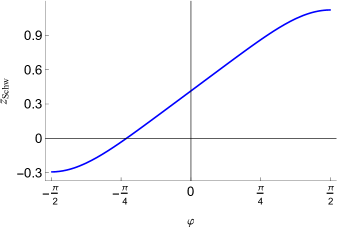
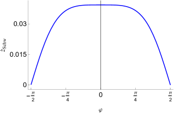
Figure 1: The frequency shift $z_{Schw}$ (left panel) and the redshift rapidity $\dot{z}_{Schw}$ (right panel) versus the azimuthal angle in the Schwarzschild background for $M=1$, $r_{e}=6$, and $D=10^{3}r_{e}$. The shift in the frequency is maximal on the midline where $\varphi=\pm\pi/2$, whereas the maximum redshift rapidity is at the line of sight $\varphi=0$. In Eqs. (10) and (23), we replaced $\delta$ with Eq. (14) to plot these curves.

In order to express the mass-to-distance ratio of the Schwarzschild black hole in terms of observational quantities, it is convenient to consider two special important cases useful for describing accretion disks revolving supermassive black holes hosted at the core of AGNs.

II.1 Midline case

The first case is related to highly shifted frequency photons emitted from particles located at the midline where $\varphi=\pm\pi/2$. The position vector of these particles with respect to the black hole center is orthogonal to the observer’s line of sight. Hence, by substituting $\varphi=\pm\pi/2$ in the frequency shift formula (10), one can find the highly redshifted ($\varphi=+\pi/2$) and blueshifted ($\varphi=-\pi/2$) photons as below

$$1+z_{{}_{Schw_{1,2}}}^{m}\!=\sqrt{\frac{r_{e}}{r_{e}-3M}}\left(1\pm\sqrt{\frac{Mr_{e}}{r_{e}-2M\cos^{2}\delta_{m}}}\cos\delta_{m}\right),$$ (15)

where the index “$m$” means the aperture angle $\delta$ should be measured on the midline and the plus (minus) sign refers to the redshifted (blueshifted) photons denoted by $z_{{}_{Schw_{1}}}^{m}$ ($z_{{}_{Schw_{2}}}^{m}$) on the midline. By multiplying $R_{m}:=1+z_{{}_{Schw_{1}}}^{m}$ and $B_{m}:=1+z_{{}_{Schw_{2}}}^{m}$, it is straightforward to obtain the mass-to-distance ratio of the Schwarzschild black hole in terms of observational quantities on the midline as follows

$$\frac{M}{D\delta_{m}}=\frac{R_{m}B_{m}-1}{2R_{m}B_{m}}-\frac{\left(1-R_{m}B_{m}\right)\left(3-4R_{m}B_{m}\right)}{6R_{m}B_{m}(3-R_{m}B_{m})}\delta_{m}^{2},$$ (16)

where we used the approximation (45) where $D\gg r_{e}$ is the radial distance between the black hole and the detector. Additionally, we considered the limit $\delta_{m}\rightarrow 0$ in consistency with the condition (4) for distant observers as well. As we can see from Eq. (16), the mass-to-distance ratio of the Schwarzschild black hole is expressed in terms of directly observational elements $\left\{R_{m},B_{m},\delta_{m}\right\}$.

II.2 Line of sight case

The second case is describing the frequency shift of photons emitted close to the line of sight where $\varphi\rightarrow 0$. Hence, by substituting $\varphi=\varphi_{s}\sim 0$ in the frequency shift formula (10), we find the expressions for slightly redshifted and slightly blueshifted photons as below

$$1+z_{{}_{Schw_{1,2}}}^{s}\!=\sqrt{\frac{r_{e}}{r_{e}-3M}}\pm\sqrt{\frac{M}{r_{e}-3M}}\left(\varphi_{s}+\delta_{s}\right),$$ (17)

where the index “$s$” means the measurement should be performed for systemic particles (particles close to the line of sight) and we applied the limit $\delta_{s}\rightarrow 0$ simultaneously. Additionally, we have just the gravitational redshift $z_{g}$ exactly at the line of sight with $\varphi_{s}=0=\delta_{s}$. In this relation, the angles $\delta_{s}$ and $\varphi_{s}$ should be measured close to the line of sight, and the plus (minus) sign refers to the redshifted (blueshifted) photons close to the line of sight denoted by $z_{{}_{Schw_{1}}}^{s}$ ($z_{{}_{Schw_{2}}}^{s}$), respectively. Now, by multiplying $R_{s}:=1+z_{{}_{Schw_{1}}}^{s}$ and $B_{s}:=1+z_{{}_{Schw_{2}}}^{s}$, we can obtain the mass-to-distance ratio of the Schwarzschild black hole close to the line of sight as follows

$$\frac{M\varphi_{s}}{D\delta_{s}}=\frac{R_{s}B_{s}-1}{3R_{s}B_{s}}+\mathcal{O}\left(\varphi_{s}^{2}\right),$$ (18)

in which we used the approximation $r_{e}\sim D\delta_{s}/\varphi_{s}$ from Eq. (46) valid close to the line of sight and considered the limits $\left\{\delta_{s}\rightarrow 0,\varphi_{s}\rightarrow 0\right\}$ simultaneously to derive this equation. Furthermore, this relation is a function of a set of purely observational quantities $\left\{R_{s},B_{s}\right\}$.

III Disentangling mass and distance

The mass-to-distance ratio formulas (16) and (18) of the Schwarzschild black hole can be employed to estimate the $M/D$ ratio of real astrophysical systems as it was accomplished for the central supermassive black holes of $17$ galaxies in ApJL ; TXS ; TenAGNs ; FiveAGNs . As the next step in this direction, we are going to disentangle the mass $M$ and the distance to the black hole $D$ to obtain closed formulas for each parameter in terms of the set of observational elements $\left\{R_{m},B_{m},\delta_{m};R_{s},B_{s},\delta_{s}\right\}$. To do so, we define the redshift rapidity as the proper time evolution of the frequency shift $z_{Schw}$ (6) in the Schwarzschild background as follows

$$\dot{z}_{Schw,e}=\frac{dz_{Schw}}{d\tau}=\frac{d}{d\tau}(U_{e}^{t}-b_{\gamma}U_{e}^{\varphi}),$$ (19)

which is the redshift rapidity at the emission point. Notwithstanding, we should note that the redshift rapidity needs to be measured from the Earth. Therefore, by making use of the chain rule, we rewrite Eq. (19) at the observer position as

$$\dot{z}_{Schw}=\frac{dz_{Schw}}{dt}=\frac{d\tau}{dt}\frac{dz_{Schw}}{d\tau}=\frac{1}{U_{e}^{t}}\frac{d}{d\tau}(U_{e}^{t}-b_{\gamma}U_{e}^{\varphi}),$$ (20)

which is an observable quantity that we measure here on the Earth. For massive geodesic particles circularly orbiting the black hole in the equatorial plane, the redshift rapidity (20) reduces to

$$\dot{z}_{Schw}=-\frac{db_{\gamma}}{d\tau}\ \frac{U_{e}^{\varphi}}{U_{e}^{t}},$$ (21)

since the $t$-component $U_{e}^{t}$ (7) and $\varphi$-component $U_{e}^{\varphi}$ (8) of the $4$-velocity are constant quantities for circular orbits whereas the light bending parameter (9) is time dependent through $\delta$ and $\varphi$. By employing the chain rule, we have

$$\dot{z}_{Schw}=-\left(\frac{\partial b_{\gamma}}{\partial\varphi}+\frac{\partial b_{\gamma}}{\partial\delta}\frac{\partial\delta}{\partial\varphi}\right)\frac{\left(U_{e}^{\varphi}\right)^{2}}{U_{e}^{t}},$$ (22)

where we used $U_{e}^{\varphi}=\left.\frac{d\varphi}{d\tau}\right|_{r=r_{e}}$. Now, we perform the aforementioned derivatives by taking into account the light bending parameter (9) and the $\delta\left(\varphi\right)$-relation (14) to obtain the redshift rapidity for an arbitrary point on the circular orbit as below

$$\dot{z}_{Schw}\!\!=\frac{1}{\left[r_{e}-2M\sin^{2}(\varphi+\text{$\delta$})\right]^{\frac{3}{2}}}\times$$

$$\frac{DM\left(D-r_{e}\cos\varphi\right)\cos(\varphi+\text{$\delta$})}{\sqrt{r_{e}-3M}\left(D^{2}+r_{e}^{2}-2Dr_{e}\cos\varphi\right)}\!.$$ (23)

Fig. 1 shows the behavior of the redshift rapidity versus the azimuthal angle $\varphi$. As one can see from this figure, the redshift rapidity at the line of sight is maximal, hence it is easier to measure this quantity at $\varphi=0$.

It is worth noting that the redshift rapidity (23) reduces to the projection of the Keplerian acceleration of a particle in circular motion on the line of sight in the Newtonian limit $M/r_{e}\rightarrow 0$ and large distances $r_{e}/D\rightarrow 0$

$$\dot{z}_{N}=\frac{M}{r_{e}^{2}}\cos(\varphi+\delta)+\mathcal{O}\left(\frac{M^{2}}{r_{e}^{3}}\right),$$ (24)

as it should be.

As the final step, based on the emitter-black hole system configuration and observational data availability, we can employ the redshift rapidity (23) as well as either Eq. (16) or Eq. (18) to disentangle the Schwarzschild black hole mass $M$ and the distance to the black hole $D$. Here, we are going to disentangle $M$ and $D$ for two important cases describing astrophysical photon sources within accretion disks circularly orbiting central supermassive black holes at the core of AGNs.

III.1 Midline case

The first important case is related to the emitters on the midline where their emitted photons are highly redshifted/blueshifted. The mass-to-distance ratio of the central black hole in terms of these frequency shifted photons is given in Eq. (16). In order to find the redshift rapidity of the same redshifted particles, we substitute the approximation (45) for $r_{e}$ in the redshift rapidity relation (23) and consider the limit $\delta_{m}\rightarrow 0$ to get

$$\dot{z}_{Schw}^{m} = \frac{\frac{M}{D\delta_{m}}}{D\sqrt{1-3\frac{M}{D\delta_{m}}}\left(1-2\frac{M}{D\delta_{m}}\right)^{\frac{3}{2}}}\times$$ (25)

$$\left(1+\frac{11-28\frac{M}{D\delta_{m}}-12\left(\frac{M}{D\delta_{m}}\right)^{2}}{6\left(1-3\frac{M}{D\delta_{m}}\right)\left(1-2\frac{M}{D\delta_{m}}\right)}\delta_{m}^{2}\right),$$

up to second order in $\delta_{m}$. Finally, one can find the explicit form of the Schwarzschild black hole mass and distance to the black hole by solving Eqs. (16) and (25) as below

$$M=\frac{\left(R_{m}B_{m}-1\right)^{2}}{2\dot{z}_{Schw}^{m}\sqrt{6-2R_{m}B_{m}}}\delta_{m}+\mathcal{O}\left(\delta_{m}^{3}\right),$$ (26)

$$D\!\!=\frac{R_{m}B_{m}\left(R_{m}B_{m}-1\right)}{\dot{z}_{Schw}^{m}\sqrt{6-2R_{m}B_{m}}}\times$$ (27)

$$\left(1+\frac{R_{m}B_{m}(3R_{m}B_{m}-7)(8R_{m}B_{m}-27)-36}{6(R_{m}B_{m}-3)^{2}}\delta_{m}^{2}\right)\!,$$

fully expressed in terms of observational quantities $\left\{R_{m},B_{m},\dot{z}_{Schw}^{m},\delta_{m}\right\}$ that should be measured on the midline.

III.2 Line of sight case

The second important case belongs to the photon sources that lie close to the line of sight where their emitted photons are slightly redshifted/blueshifted but have maximum redshift rapidity. The mass-to-distance ratio of the central black hole in terms of these frequency shifted photons is given by Eq. (18). Thus, we substitute $r_{e}=D\delta_{s}/\varphi_{s}$ from the approximation (46) into the redshift rapidity formula (23) and apply the limits $\left\{\delta_{s}\rightarrow 0,\varphi_{s}\rightarrow 0\right\}$ to get

$$\dot{z}_{Schw}^{s}=\frac{1}{M}\left(1-3\frac{M\varphi_{s}}{D\delta_{s}}\right)^{-\frac{1}{2}}\left(\frac{M\varphi_{s}}{D\delta_{s}}\right)^{2},$$ (28)

for the photon sources close to the line of sight. Now, by substituting Eq. (18) in this relation, we can find the Schwarzschild black hole mass as follows

$$M=\frac{\left(R_{s}B_{s}-1\right)^{2}}{9\dot{z}_{Schw}^{s}\left(R_{s}B_{s}\right)^{\frac{3}{2}}},$$ (29)

fully in terms of observational quantities $\left\{R_{s},B_{s},\dot{z}_{Schw}^{s}\right\}$ that should be measured close to the line of sight. As the next step, we take advantage of this relation and Eq. (16) in order to combine observations from both midline and line of sight to get the distance to the black hole as

$$D=\frac{\left(R_{s}B_{s}-1\right)^{2}}{9\dot{z}_{Schw}^{s}\left(R_{s}B_{s}\right)^{\frac{3}{2}}}\frac{2R_{m}B_{m}}{\delta_{m}\left(R_{m}B_{m}-1\right)},$$ (30)

which is a significant relation because it contains information on both high-frequency shifted particles on the midline $\left\{R_{m},B_{m}\right\}$ and maximum redshift rapidity close to the line of sight $\dot{z}_{Schw}^{s}$ (see Fig. 1 and related discussion). From an observational point of view, this formula is important due to the fact that it is easier to identify frequency shifts on the midline and the redshift rapidity close to the line of sight.

IV Discussion and final remarks

In this paper, we have presented two relations for the mass-to-distance ratio of the Schwarzschild black hole in terms of observable frequency shifts for three spacial points of the circular motion of orbiting massive particles: on the midline and close to the line of sight. Then, we calculated the derivative of the frequency shift in the Schwarzschild background with respect to proper time in order to introduce the redshift rapidity. Then, we employed the redshift rapidity to express the Schwarzschild black hole mass and its distance from the Earth just in terms of observational quantities. In this formalism, the redshift rapidity is also a general relativistic invariant observable element, indicating the proper time evolution of the frequency shift in the Schwarzschild spacetime.

We have extracted concise and elegant analytic formulas that allow us to disentangle mass and distance to the black hole in the Schwarzschild background and compute these parameters separately, not the mass-to-distance ratio that we have estimated before in ApJL ; TXS ; TenAGNs ; FiveAGNs . Our exact formulas have been obtained on the midline and close to the line of sight whereas the general relations could be employed in black hole parameter estimation studies. The next step in this research direction would be estimating the mass of supermassive Schwarzschild black holes hosted at the core of AGNs and their distance to the Earth with the help of the general relativistic formalism developed in the present paper. A task that we shall address in future works.

Appendix A ($\varphi+\delta$)-dependent light bending parameter and the angular distance $\delta$ as a function of the azimuthal angle $\varphi$

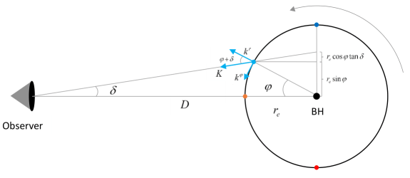
Figure 2: The geometrical illustration of the bidimensional vector $K$, and the relation between the azimuthal angle $\varphi$ and the angular distance $\delta$.

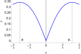
Figure 3: The profile of the angular distance versus the azimuthal angle for $D=3r_{e}$. The vertical dashed lines denote $\phi_{\pm}=\pm\arccos(1/3)$ where $d\delta/d\varphi$ vanishes.

In a similar manner to PRDbhmn , we obtain the light bending parameter for a general point of the circular orbit in the equatorial plane. However, unlike the previous work where the angular distance $\delta$ was neglected due to the large distances between the black holes and the Earth, we consider the contribution of this measurable parameter in our analysis. This is because even though the angular distance is very small, its variation with respect to time, especially close to the line of sight, is quite important. The other aim of this Appendix is to show the mathematical relation between the observable angular distance $\delta$ and the unobservable azimuthal angle $\varphi$.

In order to obtain the light bending parameter of photons coming from a general point of the circular orbit in the equatorial plane (see Fig. 2), we take into account the equation of motion of photons in the equatorial plane ($k^{\theta}=0$) of the Schwarzschild spacetime (1)

$$g_{\mu\nu}k^{\mu}k^{\nu}=g_{tt}\left(k^{t}\right)^{2}+g_{rr}\left(k^{r}\right)^{2}+g_{\varphi\varphi}\left(k^{\varphi}\right)^{2}=0,$$ (31)

where $k^{t}$ and $k^{\varphi}$ can be found through the temporal Killing vector field $\xi^{\mu}=\delta_{0}^{\mu}$ and the rotational Killing vector field $\psi^{\mu}=\delta_{3}^{\mu}$ as follows

$$E_{\gamma}=-\xi_{\mu}k^{\mu}=-g_{tt}k^{t},$$ (32)

$$L_{\gamma}=\psi_{\mu}k^{\mu}=g_{\varphi\varphi}k^{\varphi},$$ (33)

which $E_{\gamma}$ and $L_{\gamma}$ are the energy and angular momentum of the photons, respectively.

By introducing (32) and (33) into (31), the equation of motion takes the following form

$$g_{rr}\left(k^{r}\right)^{2}+\frac{E_{\gamma}^{2}}{g_{tt}}+\frac{L_{\gamma}^{2}}{g_{\varphi\varphi}}=0,$$ (34)

that can be employed to express $k^{r}$ in terms of the constants of motion and metric components as below

$$\left(k^{r}\right)^{2}=-\frac{1}{g_{rr}}\left(\frac{E_{\gamma}^{2}}{g_{tt}}+\frac{L_{\gamma}^{2}}{g_{\varphi\varphi}}\right).$$ (35)

Now, by considering the non-vanishing angular distance $\delta\neq 0$, we geometrically introduce the auxiliary bidimensional vector $K$ defined by the following decomposition (see Fig. 2 for more details)

$$k^{r}=K\cos\left(\varphi+\delta\right),$$ (36)

$$r_{e}k^{\varphi}=K\sin\left(\varphi+\delta\right),$$ (37)

with

$$K^{2}=\left(k^{r}\right)^{2}+r_{e}^{2}\left(k^{\varphi}\right)^{2}.$$ (38)

Hence, by substituting Eqs. (33) and (35) into (38), one can find $K^{2}$ versus the constants of motion and metric components as follows

$$K^{2}=-\frac{1}{g_{rr}}\left(\frac{E_{\gamma}^{2}}{g_{tt}}+\frac{L_{\gamma}^{2}}{g_{\varphi\varphi}}\right)+r_{e}^{2}\frac{L_{\gamma}^{2}}{g_{\varphi\varphi}^{2}}.$$ (39)

On the other hand, by introducing Eq. (36) into (35), we can find a similar relation for $K^{2}$ as

$$K^{2}=-\frac{1}{g_{rr}\cos^{2}\left(\varphi+\delta\right)}\left(\frac{E_{\gamma}^{2}}{g_{tt}}+\frac{L_{\gamma}^{2}}{g_{\varphi\varphi}}\right).$$ (40)

Equating previous relations gives an equation for the $\left(\varphi+\delta\right)$-dependent light bending parameter $b_{\gamma}$ as below

$$\left(g_{tt}b_{\gamma}^{2}+g_{\varphi\varphi}\right)g_{\varphi\varphi}\tan^{2}\left(\varphi+\delta\right)+r_{e}^{2}g_{rr}g_{tt}b_{\gamma}^{2}=0,$$ (41)

that leads to the following solution for $b_{\gamma}$

$$b_{\gamma}=\frac{-g_{\varphi\varphi}\sin\left(\varphi+\delta\right)}{\sqrt{-g_{tt}}\sqrt{g_{\varphi\varphi}\sin^{2}\left(\varphi+\delta\right)+r_{e}^{2}g_{rr}\cos^{2}\left(\varphi+\delta\right)}},$$ (42)

which is the light bending parameter for an arbitrary point of the circular orbit on the equatorial plane.

On the other hand, we assume the emitter is far enough from the black hole and consider the geometrical configuration illustrated in Fig. 2 to obtain a relation between the observable angular distance $\delta$ and the unobservable azimuthal angle $\varphi$. This is necessary to express $\varphi$ in terms of the observable quantity $\delta$ in order to obtain $M$ and $D$ just in terms of observational elements, hence being able to break the degeneracy of the $M/D$ ratio.

By taking into account the right triangle in Fig. 2, one can immediately identify the following relation between the set $\left\{D,r_{e};\varphi,\delta\right\}$

$$D\tan\delta=r_{e}\left(\sin\varphi+\cos\varphi\tan\delta\right),$$ (43)

where only $\delta$ is observable and the rest of the parameters are unknown in the case of black holes since we cannot identify the black hole position by observations. After doing some straightforward simplifications, this relation reduces to

$$D\sin\delta=r_{e}\sin\left(\varphi+\delta\right),$$ (44)

in which for the far away detectors where $D\gg r_{e}$ and $\delta\rightarrow 0$, we have

$$r_{e}\approx D\delta_{m}\left(1+\frac{\delta_{m}^{2}}{3}\right),\text{ \ for \ }\varphi=\pm\frac{\pi}{2},$$ (45)

$$r_{e}\approx\frac{D\delta_{s}}{\varphi_{s}},\text{ \ for \ }\varphi\rightarrow 0,$$ (46)

for the midline $\varphi=\pm\pi/2$ and close to the line of sight $\varphi\rightarrow 0$, respectively.

Now, we solve the relation (44) in order to express $\delta$ in terms of the rest of the parameters. This equality has four solutions, and we choose the physical one as below

$$\delta=\arccos\left(\frac{D-r_{e}\cos\varphi}{\sqrt{D^{2}+r_{e}^{2}-2Dr_{e}\cos\varphi}}\right),$$ (47)

since as $\varphi$ decreases/increases, $\delta$ should also decrease/increase in the same direction (see Fig. 2).

Fig. 3 illustrates the behavior of $\delta$ versus $\varphi$. As one can see from this figure, if we solve the azimuthal angle $\varphi$ in terms of $\delta$, we shall have four expressions as follows

$$\varphi=\left\{\begin{array}[]{cc}\pm\delta\mp\arcsin\left(\frac{D\sin\delta}{r_{e}}\right),&\phi_{-}\leq\varphi\leq\phi_{+}\\ \pm\pi\mp\delta\mp\arcsin\left(\frac{D\sin\delta}{r_{e}}\right),&\left\{\begin{array}[]{c}-\frac{\pi}{2}\leq\varphi\leq\phi_{-}\\ \phi_{+}\leq\varphi\leq\frac{\pi}{2}\end{array}\right.\end{array}\right.,$$ (48)

to cover the whole semicircular path from $\varphi=-\pi/2$ to $\varphi=\pi/2$. In these relations, $\phi_{+}$ ($\phi_{-}$) denotes a special point where $d\delta/d\varphi$ vanishes for $\varphi>0$ ($\varphi<0$), as indicated in Fig. 3.

References

- (1) B. P. Abbott et al. (LIGO Scientific and Virgo Collaborations), Observation of Gravitational Waves from a Binary Black Hole Merger, Phys. Rev. Lett. 116, 061102 (2016).
- (2) K. Akiyama et al. (Event Horizon Telescope Collaboration), First M87 Event Horizon Telescope Results. IV. Imaging the Central Supermassive Black Hole, Astrophys. J. Lett. 875, L4 (2019).
- (3) K. Akiyama et al. (Event Horizon Telescope Collaboration), First Sagittarius A* Event Horizon Telescope Results. VI. Testing the Black Hole Metric, Astrophys. J. Lett. 930, L17 (2022).
- (4) A. M. Ghez, S. Salim, N. N. Weinberg, J. R. Lu, T. Do, J. K. Dunn, K. Matthews, M. R. Morris, S. Yelda, E. E. Becklin, T. Kremenek, M. Milosavljevic and J. Naiman, Measuring Distance and Properties of the Milky Way’s Central Supermassive Black Hole with Stellar Orbits, Astrophys. J. 689, 1044 (2008).
- (5) M. R. Morris, L. Meyer and A. M. Ghez, Galactic center research: manifestations of the central black hole, Res. Astron. Astrophys. 12, 995 (2012).
- (6) A. Eckart and R. Genzel, Observations of stellar proper motions near the Galactic Centre, Nature 383, 415 (1996).
- (7) S. Gillessen, F. Eisenhauer, S. Trippe, T. Alexander, R. Genzel, F. Martins and T. Ott, Monitoring stellar orbits around the massive black hole in the galactic center, Astrophys. J. 692, 1075 (2009).
- (8) A. Herrera-Aguilar and U. Nucamendi, Kerr black hole parameters in terms of the redshift/blueshift of photons emitted by geodesic particles, Phys. Rev. D 92, 045024 (2015).
- (9) P. Banerjee, A. Herrera-Aguilar, M. Momennia and U. Nucamendi, Mass and spin of Kerr black holes in terms of observational quantities: The dragging effect on the redshift, Phys. Rev. D 105, 124037 (2022).
- (10) M. Momennia, A. Herrera-Aguilar and U. Nucamendi, Kerr black hole in de Sitter spacetime and observational redshift: Toward a new method to measure the Hubble constant, Phys. Rev. D 107, 104041 (2023).
- (11) J. R. Herrnstein, J. M. Moran, L. J. Greenhill and A. S. Trotter, The Geometry of and Mass Accretion Rate through the Maser Accretion Disk in NGC 4258, Astrophys. J. 629, 719 (2005).
- (12) A. L. Argon, L. J. Greenhill, M. J. Reid, J. M. Moran and E. M. L. Humphrey, Toward a new geometric distance to the active Galaxy NGC 4258. I. VLBI monitoring of water maser emission, Astrophys. J. 659, 1040 (2007).
- (13) E. M. L. Humphreys, M. J. Reid, J. M. Moran, L. J. Greenhill and A. L. Argon, Toward a new geometric distance to the active galaxy NGC 4258. III. Final results and the Hubble constant, Astrophys. J. 775, 13 (2013).
- (14) G. V. Kraniotis, Gravitational redshift/blueshift of light emitted by geodesic test particles, frame-dragging and pericentre-shift effects, in the Kerr-Newman-de Sitter and Kerr-Newman black hole geometries, Eur. Phys. J. C 81, 147 (2021).
- (15) D. Ujjal, Motion and collision of particles near Plebanski-Demianski black hole: Shadow and gravitational lensing, Chin. J. Phys. 70, 213 (2021).
- (16) M. Sharif and S. Iftikhar, Dynamics of particles near black hole with higher dimensions, Eur. Phys. J. C 76, 404 (2016).
- (17) R. Becerril, S. Valdez-Alvarado, U. Nucamendi, P. Sheoran and J. M. Davila, Mass parameter and the bounds on redshifts and blueshifts of photons emitted from geodesic particle orbiting in the vicinity of regular black holes, Phys. Rev. D 103, 084054 (2021).
- (18) P. Sheoran, A. Herrera-Aguilar and U. Nucamendi, Mass and spin of a Kerr black hole in modified gravity and a test of the Kerr black hole hypothesis, Phys. Rev. D 97, 124049 (2018).
- (19) L. A. Lopez and J. C. Olvera, Frequency shifts of photons emitted from geodesics of nonlinear electromagnetic black holes, Eur. Phys. J. Plus 136, 64 (2021).
- (20) L. A. Lopez and N. Breton, Redshift of light emitted by particles orbiting a black hole immersed in a strong magnetic field, Astrophys. Space Sci. 366, 55 (2021).
- (21) R. Becerril, S. Valdez-Alvarado and U. Nucamendi, Obtaining mass parameters of compact objects from red-blue shifts emitted by geodesic particles around them, Phys. Rev. D 94, 124024 (2016).
- (22) Q. M. Fu and X. Zhang, Probing a polymerized black hole with the frequency shifts of photons, Phys. Rev. D 107, 064019 (2023).
- (23) D. A. Martinez-Valera, M. Momennia and A. Herrera-Aguilar, Observational redshift from general spherically symmetric black holes, [arXiv:2311.17993].
- (24) U. Nucamendi, A. Herrera-Aguilar, R. Lizardo-Castro and O. Lopez-Cruz, Toward the gravitational redshift detection in NGC 4258 and the estimation of its black hole mass-to-distance ratio, Astrophys. J. Lett. 917, L14 (2021).
- (25) A. Villalobos-Ramirez, O. Gallardo-Rivera, A. Herrera-Aguilar and U. Nucamendi, A general relativistic estimation of the black hole mass-to-distance ratio at the core of TXS 2226-184, Astron. Astrophys. 662, L9 (2022).
- (26) D. Villaraos, A. Herrera-Aguilar, U. Nucamendi, G. Gonzalez-Juarez and R. Lizardo-Castro, A general relativistic mass-to-distance ratio for a set of megamaser AGN black holes, MNRAS 517, 4213 (2022).
- (27) A. Villalobos-Ramirez, A. Gonzalez-Juarez, M. Momennia and A. Herrera-Aguilar, A general relativistic mass-to-distance ratio for a set of megamaser AGN black holes II, [arXiv:2211.06486].
- (28) J. A. Braatz, M. J. Reid, E. M. L. Humphreys, C. Henkel, J. J. Condon and K. Y. Lo, The megamaser cosmology project. II. The angular-diameter distance to UGC 3789, Astrophys. J. 718, 657 (2010).
- (29) C. Y. Kuo, J. A. Braatz, M. J. Reid, K. Y. Lo, J. J. Condon, C. M. V. Impellizzeri and C. Henkel, The megamaser cosmology project. V. An angular-diameter distance to NGC 6264 at 140 Mpc, Astrophys. J. 767, 155 (2013).
- (30) F. Gao, J. A. Braatz, M. J. Reid, K. Y. Lo, J. J. Condon, C. Henkel, C. Y. Kuo, C. M. V. Impellizzeri, D. W. Pesce and W. Zhao, The megamaser cosmology project. VIII. A geometric distance to NGC 5765b, Astrophys. J. 817, 128 (2016).
- (31) M. J. Reid, D. W. Pesce and A. G. Riess, An improved distance to NGC 4258 and its implications for the Hubble constant, Astrophys. J. Lett. 886, L27 (2019).
- (32) D. W. Pesce, J. A. Braatz, M. J. Reid, J. J. Condon, F. Gao, C. Henkel, C. Y. Kuo, K. Y. Lo and W. Zhao, The Megamaser Cosmology Project. XI. A Geometric Distance to CGCG 074-064, Astrophys. J. 890, 118 (2020).