Neural Entropic Gromov-Wasserstein Alignment

Abstract.

The Gromov-Wasserstein (GW) distance, rooted in optimal transport (OT) theory, provides a natural framework for aligning heterogeneous datasets. Alas, statistical estimation of the GW distance suffers from the curse of dimensionality and its exact computation is NP hard. To circumvent these issues, entropic regularization has emerged as a remedy that enables parametric estimation rates via plug-in and efficient computation using Sinkhorn iterations. Motivated by further scaling up entropic GW (EGW) alignment methods to data dimensions and sample sizes that appear in modern machine learning applications, we propose a novel neural estimation approach. Our estimator parametrizes a minimax semi-dual representation of the EGW distance by a neural network, approximates expectations by sample means, and optimizes the resulting empirical objective over parameter space. We establish non-asymptotic error bounds on the EGW neural estimator of the alignment cost and optimal plan. Our bounds characterize the effective error in terms of neural network (NN) size and the number of samples, revealing optimal scaling laws that guarantee parametric convergence. The bounds hold for compactly supported distributions, and imply that the proposed estimator is minimax-rate optimal over that class. Numerical experiments validating our theory are also provided.

1. Introduction

The Gromov-Wasserstein (GW) distance, proposed in [Mém11], quantifies discrepancy between probability distributions supported on (possibly) distinct metric spaces. Specifically, given two metric measure (mm) spaces $\left(\mathcal{X},\mathsf{d}_{\mathcal{X}},\mu\right)$ and $\left(\mathcal{Y},\mathsf{d}_{\mathcal{Y}},\nu\right)$, the $(p,q)$-GW distance between them is

$$\mathsf{D}_{p,q}(\mu,\nu)\coloneqq\inf_{\pi\in\Pi(\mu,\nu)}\left(\int_{\mathcal{X}\times\mathcal{Y}}\int_{\mathcal{X}\times\mathcal{Y}}\left|\mathsf{d}_{\mathcal{X}}\left(x,x^{\prime}\right)^{q}-\mathsf{d}_{\mathcal{Y}}\left(y,y^{\prime}\right)^{q}\right|^{p}d\pi\otimes\pi\left(x,y,x,y^{\prime}\right)\right)^{\frac{1}{p}}$$ (1)

where $\Pi(\mu,\nu)$ is the set of all couplings between $\mu$ and $\nu$. This approach, which is based on optimal transport (OT) theory [V⁺09], serves as a relaxation of the Gromov-Hausdorff distance between metric spaces and defines a metric on the space of all mm spaces quotiented by measure preserving isometries. From an applied standpoint, a solution to the GW problem between two heterogeneous datasets yields not only a quantification of discrepancy, but also an optimal matching $\pi_{\star}$ between them. As such, alignment methods inspired by the GW problem have been proposed for many applications, encompassing single-cell genomics [DSS⁺20, BCM⁺20], alignment of language models [AMJ18], shape matching [DSS⁺20, Mém09], graph matching [XLZD19], heterogeneous domain adaptation [YLW⁺18], and generative modelling [BAMKJ19].

Despite this empirical progress, the aforementioned methods are largely heuristic and lack formal guarantees due to the statistical and computational hardness of the GW problem. Indeed, estimation of the GW distance suffers from the curse of dimensionality [ZGMS22], whereby convergence rates deteriorate exponentially with the dimension. Computationally, the GW problem is equivalent to a quadratic assignment problem (QAP), whose exact solution is NP complete [Com05]. To circumvent these issues, entropic regularization has emerged as a popular alternative [SPKS16, PCS16]:

$$\mathsf{S}_{p,q}^{\varepsilon}(\mu,\nu)\coloneqq\inf_{\pi\in\Pi\left(\mu,\nu\right)}\int\left|\mathsf{d}_{\mathcal{X}}\left(x,x^{\prime}\right)^{q}-\mathsf{d}_{\mathcal{Y}}\left(y,y^{\prime}\right)^{q}\right|^{p}d\pi\otimes\pi\left(x,y,x^{\prime},y^{\prime}\right)+\varepsilon\mathsf{D}_{\mathsf{KL}}(\pi\|\mu\otimes\nu),$$ (2)

where $\mathsf{D}_{\mathsf{KL}}$ is the Kullback-Leibler divergence. Recently, [ZGMS22] derived a novel variational representation of the entropic GW (EGW) distance that connected it to the well-understood entropic OT (EOT) problem, which unlocked powerful tools for analysis. This enabled establishing parametric estimation rates for the EGW distance [ZGMS22], as well as developing first-order methods for computing it subject to non-asymptotic convergence guarantees [RGK23]. While these new algorithms are the first to provide formal guarantees, they rely on a Sinkhorn oracle [Cut13], whose quadratic time complexity is prohibitive when dealing with large and high-dimensional datasets that appear in modern machine learning tasks. Motivated to scale up GW alignment methods to such regimes, this work develops a novel neural estimation approach that is end-to-end trainable via backpropagation, compatible with minibatch-based optimization, and adheres to strong performance guarantees.

1.1. Contributions

We focus on the nominal case of the quadratic EGW distance, i.e., when $p=q=2$, between Euclidean mm spaces $\left(\mathbb{R}^{d_{x}},\|\cdot\|,\mu\right)$ and $\left(\mathbb{R}^{d_{y}},\|\cdot\|,\nu\right)$ of possibly different dimensions. Thanks to the recently developed EGW variational representation from [ZGMS22, Theorem 1] and the EOT semi-dual form, we have

$$\mathsf{S}_{2,2}^{\varepsilon}(\mu,\nu)=\mathsf{C}_{\mu,\nu}+\inf_{\mathbf{A}\in\mathcal{D}_{M_{\mu,\nu}}}\left\{32\|\mathbf{A}\|_{\mathrm{F}}^{2}+\sup_{\varphi\in L^{1}(\mu)}\mathbb{E}_{\mu}[\varphi]+\mathbb{E}_{\nu}[\varphi^{c_{\mathbf{A},\varepsilon}}]\right\},$$ (3)

where $\mathsf{C}_{\mu,\nu}$ is a constant that depends only on the marginals (and is easy to estimate; see (10) ahead), $\mathcal{D}_{M_{\mu,\nu}}\subsetneq\mathbb{R}^{d_{x}\times d_{y}}$ is compact whenever $\mu,\nu$ have finite 2nd moments, and $\varphi^{c_{\mathbf{A},\varepsilon}}$ is $(c,\varepsilon)$-transform of $\varphi$ (cf. (7)) with respect to (w.r.t.) the cost function $c_{\mathbf{A}}(x,y)=-4\|x\|^{2}\|y\|^{2}-32x^{\intercal}\mathbf{A}y$. We study regularity of optimal dual potentials $\varphi$ and show that they belong to a Hölder class of arbitrary smoothness, uniformly in $\mathbf{A}\in\mathcal{D}_{M_{\mu,\nu}}$. Leveraging this, we define our neural estimator (NE) by parametrizing dual potentials using a neural network (NN), approximating expectations by sample means, and employing an alternating routine to optimize over the $\mathbf{A}$ matrices and the NN parameters. Our approach yields not only an estimate of the EGW distance but also a neural alignment plan that is induced by the learned NN. As the estimator is trainable via gradient methods using backpropagation and minibatches, it can seamlessly integrate into downstream tasks as a loss, a regularizer, or an alignment module.

We provide formal guarantees on the quality of the NE of the EGW cost and the corresponding alignment plan. Our analysis relies on non-asymptotic function approximation theorems and tools from empirical process theory to bound the two sources of error involved: function approximation and empirical estimation. Given $n$ samples from the population distributions, we show that the effective error of a NE realized by a shallow NN of $k$ neurons scales as

$$O\left(\mathrm{poly}(1/\varepsilon)\big{(}k^{-1/2}+n^{-1/2}\big{)}\right),$$ (4)

with the polynomial dependence on $1/\varepsilon$ explicitly characterized (see Theorems 1-3). This bound on the EGW cost estimation error holds for arbitrary, compactly supported distributions. This stands in struck contrast to existing neural estimation error bounds for other divergences [NWJ10, AMJ18, SG22, GGNR22, TGG23], which typically require strong regularity assumptions on the population distributions (e.g., Hölder smoothness of densities). This is unnecessary in our setting thanks to the inherit regularity of dual EOT potentials for smooth cost functions, which our $c_{\mathbf{A}}$ cost indeed is.

The above bound reveals the optimal scaling of the NN and dataset sizes, namely $k\asymp n$, which achieves the parametric convergence rate of $n^{-1/2}$ and guarantees minimax-rate optimality of our NE. The explicitly characterized polynomial dependence on $\varepsilon$ in our bound matches the bounds for EGW estimation via empirical plug-in [ZGMS22, GH23] (as well as analogous results for entropic OT (EOT); cf. [MNW19]). We also note that our neural estimation results readily extend to the inner product EGW distance and the EOT problem with general cost functions. The developed NE is empirically tested on synthetic and real-world datasets, demonstrating its scalability to high dimensions and validating our theory.

1.2. Related Literature

Several reformulations have been proposed to alleviate the computational intractability of the GW problem. The sliced GW distance [VFT⁺19] seeks to reduce the computational burden by averaging GW costs between one-dimensional projections of the marginal distributions. The utility of this approach, however, is contingent on resolving the GW problem on $\mathbb{R}$, which remains open [BHS23]. The unbalanced GW distance was proposed in [SVP21], along with a computationally tractable convex relaxation thereof. A Gromov-Monge map-type formulation was explored in [ZMGS22], which directly optimizes over bi-directional maps to attain structured solutions. Yet, it is the entropically regularized GW distance [PCS16, SPKS16] that has been widely adopted in practice, thanks to its compatibility with iterative methods based on Sinkhorn’s algorithm [Cut13]. Under certain low-rank assumptions on the cost matrix, [SPC22] presented an adaptation of the mirror descent approach from [PCS16] that speeds up its runtime from $O(n^{3})$ to $O(n^{2})$. More recently, [RGK23] proposed an accelerated first-order method based on the dual formulation from (3) and derived non-asymptotic convergence guarantees for it. To the best of our knowledge, the latter is the only algorithm for computing a GW variant subject to formal convergence claims. However, all the above EGW methods use iterates that run Sinkhorn’s algorithm, whose time and memory complexity scale quadratically with $n$. This hinders applicability to large-scale problems.

Neural estimation is a popular approach for enhancing scalability. Prior research explored the tradeoffs between approximation and estimation errors in non-parametric regression [Bar94, Bac17, Suz18] and density estimation [YB99, USP19] tasks. More recently, neural estimation of statistical divergences and information measures has been gaining attention. The mutual information NE (MINE) was proposed in [BBR⁺18], and has seen various improvements since [POvdO⁺18, SE19, CABH⁺19, MMD⁺21]. Extensions of the neural estimation approach to directed information were studied in [MGBS21, TAGP23b, TAGP23a]. Theoretical guarantees for $f$-divergence NEs, accounting for approximation and estimation errors, as we do here, were developed in [SSG21, SG22] (see also [NWJ10] for a related approach based on reproducing kernel Hilbert space parameterization). Neural methods for approximate computation of the Wasserstein distances have been considered under the Wasserstein generative adversarial network (GAN) framework [ACB17, GAA⁺17], although these approaches are heuristic and lack formal guarantees. Utilizing entropic regularization, [DMH21] studied a score-based generative neural EOT model, while an energy-based model was considered in [MKB23].

2. Background and Preliminaries

2.1. Notation

Let $\|\cdot\|$ denote the Euclidean norm and $\langle\cdot,\cdot\rangle$ designate the inner product. The Euclidean ball is designated as $B_{d}(r)\coloneqq\{x\in\mathbb{R}^{d}:\|x\|<r\}$. We use $\|\cdot\|_{\operatorname{op}}$ and $\|\cdot\|_{\mathrm{F}}$ for the operator and Frobenius norms of matrices, respectively. For $1\leq p<\infty$, the $L^{p}$ space over $\mathcal{X}\subseteq\mathbb{R}^{d}$ with respect to (w.r.t.) the measure $\mu$ is denoted by $L^{p}(\mu)$, with $\|\cdot\|_{p,\mu}$ representing the norm. For $p=\infty$, we use $\|\cdot\|_{\infty,\mathcal{X}}$ for standard sup-norm on $\mathcal{X}\subseteq\mathbb{R}^{d}$. Slightly abusing notation, we also set $\|\mathcal{X}\|\coloneqq\sup_{x\in\mathcal{X}}\|x\|_{\infty}$.

The class of Borel probability measures on $\mathcal{X}\subseteq\mathbb{R}^{d}$ is denoted by $\mathcal{P}(\mathcal{X})$. To stress that the expectation of $f$ is taken w.r.t. $\mu\in\mathcal{P}(\mathcal{X})$, we write $\mathbb{E}_{\mu}[f]\coloneqq\int fd\mu$. For $\mu,\nu\in\mathcal{P}(\mathcal{X})$ with $\mu\ll\nu$, i.e., $\mu$ is absolutely continuous w.r.t. $\nu$, we use $\frac{d\mu}{d\nu}$ for the Radon-Nikodym derivative of $\mu$ w.r.t. $\nu$. The subset of probability measures that are absolutely continuous w.r.t. Lebesgue is denoted by $\mathcal{P}_{\mathsf{ac}}(\mathcal{X})$. For $p\in[1,\infty)$, further let $\mathcal{P}_{p}(\mathcal{X})\subseteq\mathcal{P}(\mathcal{X})$ contain only measures with finite $p$-th absolute moment, i.e., $M_{p}(\mu)\coloneqq\int_{\mathcal{X}}\|x\|^{p}d\mu(x)<\infty$ for any $\mu\in\mathcal{P}_{p}(\mathcal{X})$.

For any multi-index $\alpha=(\alpha_{1},\dots,\alpha_{d})\in\mathbb{N}_{0}^{d}$ with $|\alpha|=\sum_{j=1}^{d}\alpha_{j}$ ($\mathbb{N}_{0}=\mathbb{N}\cup\{0\}$), define the differential operator $D^{\alpha}=\frac{\partial^{|\alpha|}}{\partial x_{1}^{\alpha_{1}}\cdots\partial x_{d}^{\alpha{}_{d}}}$ with $D^{0}f=f$. We write $N(\delta,\mathcal{F},\mathsf{d})$ for the $\delta$-covering number of a function class $\mathcal{F}$ w.r.t. a metric $\mathsf{d}$, and $N_{[\,]}(\delta,\mathcal{F},\mathsf{d})$ for the bracketing number. For an open set $\mathcal{U}\subseteq\mathbb{R}^{d}$, $b\geq 0$, and an integer $m\geq 0$, let $\mathcal{C}_{b}^{m}(\mathcal{U})\coloneqq\big{\{}f\in\mathcal{C}^{m}(\mathcal{U}):\,\max_{\alpha:|\alpha|\leq m}\left\|D^{\alpha}f\right\|_{\infty,\mathcal{U}}\leq b\big{\}}$ denote the Hölder space of smoothness index $m$ and radius $b$. The restriction of $f:\mathbb{R}^{d}\rightarrow\mathbb{R}$ to a subset $\mathcal{X}\subseteq\mathbb{R}^{d}$ is denoted by $f\big{|}_{\mathcal{X}}$. We use $\lesssim_{x}$ to denote inequalities up to constants that only depend on $x$; the subscript is dropped when the constant is universal. For $a,b\in\mathbb{R}$, we use the shorthands $a\vee b=\max\{a,b\}$ and $a\land b=\min\{a,b\}$.

2.2. Entropic Optimal Transport

Our NE of the EGW distance leverages the dual formulation form [ZGMS22], which represents it in terms of a class of entropically regularized OT problems. We therefore start by setting up EOT. Given distributions $(\mu,\nu)\in\mathcal{P}(\mathcal{X})\times\mathcal{P}(\mathcal{Y})$ and a cost function $c:\mathcal{X}\times\mathcal{Y}\to\mathbb{R}$, the primal EOT formulation is obtained by regularizing the OT cost by the KL divergence,

$$\mathsf{OT}_{c}^{\varepsilon}(\mu,\nu)\coloneqq\inf_{\gamma\in\Pi(\mu,\nu)}\int c\,d\gamma+\varepsilon\mathsf{D}_{\mathsf{KL}}(\gamma\|\mu\otimes\nu),$$ (5)

where $\varepsilon>0$ is a regularization parameter and $\mathsf{D}_{\mathsf{KL}}(\mu\|\nu)\coloneqq\int\log\left(\frac{d\mu}{d\nu}\right)d\mu$ if $\mu\ll\nu$ and $+\infty$ otherwise. Classical OT [Vil08, San15] is obtained from (5) by setting $\varepsilon=0$. When $c\in L^{1}(\mu\otimes\nu)$, EOT admits the dual and semi-dual formulations, which are, respectively, given by

$$\mathsf{OT}_{c}^{\varepsilon}(\mu,\nu) =\sup_{(\varphi,\psi)\in L^{1}(\mu)\times L^{1}(\nu)}\int\varphi d\mu+\int\psi d\nu-\varepsilon\int e^{\frac{\varphi\oplus\psi-c}{\varepsilon}}d\mu\otimes\nu+\varepsilon,$$ (6)

$$=\sup_{\varphi\in L^{1}(\mu)}\int\varphi d\mu+\int\varphi^{c,\varepsilon}d\nu,$$ (7)

where we have defined $(\varphi\oplus\psi)(x,y)=\varphi(x)+\psi(y)$ and the $(c,\varepsilon)$-transform of $\varphi$ is given by $\varphi^{c,\varepsilon}=-\varepsilon\log\left(\int_{\mathcal{X}}\exp\left(\frac{\varphi(x)-c(x,\cdot)}{\varepsilon}\right)d\mu(x)\right)$. There exist functions $(\varphi,\psi)$ that achieve the supremum in $\eqref{eq:EOT_dual}$, which we call EOT potentials. These potentials are almost surely (a.s.) unique up to additive constants, i.e., if $(\tilde{\varphi},\tilde{\psi})$ is another pair of EOT potentials, then there exists a constant $a\in\mathbb{R}$ such that $\tilde{\varphi}=\varphi+a$ $\mu$-a.s. and $\tilde{\psi}=\psi-a$ $\nu$-a.s.

A pair $(\varphi,\psi)\in L^{1}(\mu)\times L^{1}(\nu)$ are EOT potentials if and only if they satisfy the Schrödinger system

$$\int e^{\frac{\varphi(x)+\psi(\cdot)-c(x,\cdot)}{\varepsilon}}d\mu(x)=1\quad\nu\text{-a.s. }\quad\text{ and }\quad\int e^{\frac{\varphi(\cdot)+\psi(y)-c(\cdot,y)}{\varepsilon}}d\nu(y)=1\quad\mu\text{-a.s. }$$ (8)

Furthermore, $\varphi$ solves the semi-dual from (7) if an only if $(\varphi,\varphi^{c,\varepsilon})$ is a solution to the full dual in (6). Given EOT potentials $(\varphi,\psi)$, the unique EOT plan can be expressed in their terms as $d\gamma^{\varepsilon}_{\star}=$ $e^{\frac{\varphi\oplus\psi-c}{\varepsilon}}d\mu\otimes\nu$. Subject to smoothness assumptions on the cost function and the population distributions, various regularity properties of EOT potentials can be derived; cf., e.g., [GKRS22, Lemma 1].

2.3. Entropic Gromov-Wasserstein Distance

We consider the quadratic EGW distance (i.e., when $p=q=2$) between Euclidean mm spaces $(\mathbb{R}^{d_{x}},\|\cdot\|,\mu)$ and $(\mathbb{R}^{d_{y}},\|\cdot\|,\nu)$, where $\mu,\nu$ are assumed to have finite 4th absolute moments:

$$\mathsf{S}^{\varepsilon}(\mu,\nu)\coloneqq\mathsf{S}_{2,2}^{\varepsilon}(\mu,\nu)=\inf_{\pi\in\Pi(\mu,\nu)}\int\left|\|x-x^{\prime}\|^{2}-\|y-y^{\prime}\|^{2}\right|^{2}d\pi\otimes\pi(x,y,x^{\prime},y^{\prime})+\varepsilon\mathsf{D}_{\mathsf{KL}}(\pi\|\mu\otimes\nu).$$ (9)

By a standard compactness argument, the infimum above is always achieved, and we call such a solution an optimal EGW alignment plan, denoted by $\pi_{\star}^{\varepsilon}$ [Mém11]. By analogy to OT, EGW serves as a proxy of the standard GW distance up to an additive gap of $O\big{(}\varepsilon\log(1/\varepsilon)\big{)}$ [ZGMS22]. One readily verifies that, like the unregularized distance, EGW is invariant to isometric actions on the marginal spaces such as orthogonal rotations and translations.

It was shown in [ZGMS22, Theorem 1] that when $\mu,\nu$ are centered, which we may assume without loss of generality, the EGW cost admits a dual representation. To state it, define

$$\mathsf{C}(\mu,\nu)\coloneqq\int\|x-x^{\prime}\|^{4}d\mu\otimes\mu(x,x^{\prime})+\int\|y-y^{\prime}\|^{4}d\nu\otimes\nu(y,y^{\prime})-4\int\|x\|^{2}\|y\|^{2}d\mu\otimes\nu(x,y),$$ (10)

which, evidently, depends only on the marginals $\mu,\nu$. We have the following.

Lemma 1 (EGW duality; Theorem 1 in [ZGMS22]).

Fix $\varepsilon>0$, $(\mu,\nu)\in\mathcal{P}_{4}(\mathbb{R}^{d_{x}})\times\mathcal{P}_{4}(\mathbb{R}^{d_{y}})$ with zero mean, and let $M_{\mu,\nu}\coloneqq\sqrt{M_{2}(\mu)M_{2}(\nu)}$. Then,

$$\mathsf{S}^{\varepsilon}(\mu,\nu)=\mathsf{C}(\mu,\nu)+\inf_{\mathbf{A}\in\mathbb{R}^{d_{x}\times d_{y}}}\Big{\{}32\|\mathbf{A}\|_{\mathrm{F}}^{2}+\mathsf{OT}_{\mathbf{A}}^{\mspace{1.0mu}\varepsilon}(\mu,\nu)\Big{\}},$$ (11)

where $\mathsf{OT}_{\mathbf{A}}^{\mspace{1.0mu}\varepsilon}$ is the EOT problem with cost $c_{\mathbf{A}}:(x,y)\in\mathbb{R}^{d_{x}}\times\mathbb{R}^{d_{y}}\mapsto-4\|x\|^{2}\|y\|^{2}-32x^{\intercal}\mathbf{A}y$. Moreover, the infimum is achieved at some $\mathbf{A}_{\star}\in\mathcal{D}_{M_{\mu,\nu}}\coloneqq[-M_{\mu,\nu}/2,M_{\mu,\nu}/2]^{d_{x}\times d_{y}}$.

Although (11) illustrates a connection between the EGW and EOT problems, the outer minimization over $\mathbf{A}$ necessitates studying EOT with an a priori unknown cost function $c_{\mathbf{A}}$, which depends on the considered distributions. To enable that, in Lemma 2 ahead we show that there exist smooth EOT potentials $(\varphi_{\mathbf{A}},\varphi_{\mathbf{A}}^{c,\varepsilon})$ for $\mathsf{OT}_{\mathbf{A}}^{\mspace{1.0mu}\varepsilon}(\mu,\nu)$ satisfying certain derivative estimates uniformly in $\mathbf{A}\in\mathcal{D}_{M}$ (for some $M\geq M_{\mu,\nu}$) and $\mu,\nu$. This enables accurately approximating them by NNs and, in turn, unlocks our neural estimation approach.

Remark 1 (Inner product cost).

The NE approach developed in the next section for the quadratic EGW distance extends almost directly to the case of the inner product distortion cost (abbreviated henceforth by IEGW)"

$$\mathsf{F}^{\varepsilon}(\mu,\nu)=\inf_{\pi\in\Pi(\mu,\nu)}\int\left|\langle x,x^{\prime}\rangle-\langle y,y^{\prime}\rangle\right|^{2}d\pi\otimes\pi(x,y,x^{\prime},y^{\prime})+\varepsilon\mathsf{D}_{\mathsf{KL}}(\pi\|\mu\otimes\nu).$$ (12)

The cost function above is not a distance distortion measure; rather, it quantifies the change in angles. This object has received recent attention due to its analytic tractability [LLN⁺22] and since it captures a meaningful notion of discrepancy between mm spaces with a natural inner product structure. IEGW enjoys a similar decomposition, dual representation, and regularity of dual potentials as its quadratic counterpart. As such, it falls under our neural estimation framework and can be treated similarly. To avoid repetition, we collect the results pertaining to the IEGW distance in Appendix A.

3. Neural Estimation of the EGW Alignment Cost and Plan

We consider compactly supported distributions $(\mu,\nu)\in\mathcal{P}(\mathcal{X})\times\mathcal{P}(\mathcal{X})$, and assume, for simplicity, that $\mathcal{X}\subseteq[-1,1]^{d_{x}}$ and $\mathcal{Y}\subseteq[-1,1]^{d_{y}}$ (our results readily extend to arbitrary compact supports in Euclidean mm spaces). Without loss of generality, further suppose that $\mu$ and $\nu$ are centered (due to translation invariance) and that $d_{x}\leq d_{y}$. We next describe the NE for the EGW distance and provide non-asymptotic performance guarantees for estimation both the alignment cost and plan. All proofs are deferred to the supplement.

3.1. EGW Neural Estimator

For $(\mu,\nu)\in\mathcal{P}(\mathcal{X})\times\mathcal{P}(\mathcal{Y})$, let $X^{n}\coloneqq\left(X_{1},\cdots,X_{n}\right)$ and $Y^{n}\coloneqq\left(Y_{1},\cdots,Y_{n}\right)$ be $n$ independently and identically distributed (i.i.d.) samples from $\mu$ and $\nu$, respectively. Further suppose that the sample sets are independent of each other. Denote the empirical measures induced by these samples as $\hat{\mu}_{n}=n^{-1}\sum_{i=1}^{n}\delta_{X_{i}}$ and $\hat{\nu}_{n}=n^{-1}\sum_{i=1}^{n}\delta_{Y_{i}}$.

Our NE is realized by a shallow ReLU NN (i.e., with a single hidden layer) with $k$ neurons, which defines the function class

$$\mathcal{F}_{k,d}(a)\coloneqq\left\{f:\mathbb{R}^{d}\rightarrow\mathbb{R}:\begin{aligned} &f(x)=\sum_{i=1}^{k}\beta_{i}\phi\left(w_{i}\cdot x+b_{i}\right)+w_{0}\cdot x+b_{0},\\ &\max_{1\leq i\leq k}\left\|w_{i}\right\|_{1}\vee\left|b_{i}\right|\leq 1,\ \max_{1\leq i\leq k}\left|\beta_{i}\right|\leq 2ak^{-1},\ \left|b_{0}\right|\leq a,\ \left\|w_{0}\right\|_{1}\leq a\end{aligned}\right\},$$ (13)

where $a\in\mathbb{R}_{\geq 0}$ specifies the parameter bounds and $\phi:\mathbb{R}\to\mathbb{R}_{\geq 0}:z\mapsto z\vee 0$ is the ReLU activation function, which acts on vectors component-wise.

Consider the variational representation of the EGW distance stated in Lemma 1. The constant $\mathsf{C}(\mu,\nu)$ involves only moments of the marginal distributions and, as such, we estimate it using empirical averages via $\widehat{\mathsf{C}}(X^{n},Y^{n})\coloneqq\mathsf{C}(\hat{\mu}_{n},\hat{\nu}_{n})$. For the remaining term, we parametrize the semi-dual form of $\mathsf{OT}_{\mathbf{A}}^{\mspace{1.0mu}\varepsilon}(\mu,\nu)$ (see (7)) using a NN from the class $\mathcal{F}_{k,d}(a)$ and replace expectations with sample means. Recalling that $d_{x}\leq d_{y}$, define

$$\widehat{\mathsf{OT}}_{\mathbf{A},k,a}^{\mspace{1.0mu}\varepsilon}(X^{n},Y^{n})\coloneqq\max_{f\in\mathcal{F}_{k,d_{x}}(a)}\frac{1}{n}\sum_{i=1}^{n}f(X_{i})-\frac{\varepsilon}{n}\sum_{j=1}^{n}\log\left(\frac{1}{n}\sum_{i=1}^{n}\exp\left(\frac{f(X_{i})-c_{\mathbf{A}}(X_{i},Y_{j})}{\varepsilon}\right)\right).$$ (14)

Inserting these estimates back into the representation from (11), the EGW distance NE is given by

$$\widehat{\mathsf{S}}_{k,a}^{\mspace{1.0mu}\varepsilon}(X^{n},Y^{n})\coloneqq\widehat{\mathsf{C}}(X^{n},Y^{n})+\inf_{\mathbf{A}\in\mathcal{D}_{M}}\Big{\{}32\|\mathbf{A}\|_{\mathrm{F}}^{2}+\widehat{\mathsf{OT}}_{\mathbf{A},k,a}^{\mspace{1.0mu}\varepsilon}(X^{n},Y^{n})\Big{\}}.$$ (15)

where $M=\sqrt{d_{x}d_{y}}$. This choice is based on the fact that $\sqrt{d_{x}d_{y}}\geq M_{\mu,\nu}\vee M_{\hat{\mu}_{n},\hat{\nu}_{n}}$ and the right-hand side (RHS) of (11) achieves its global minimum inside $\mathcal{D}_{M_{\mu,\nu}}$. This estimator can be computed via alternating optimization over the matrices $\mathbf{A}$ and the NN parameters.

For any pair $(\mathbf{A},f)\in\mathcal{D}_{M}\times\mathcal{F}_{k,d_{x}}(a)$, we define the induced neural alignment plan

$$d\pi^{\varepsilon}_{\mathbf{A},f}(x,y)\coloneqq\frac{\exp\left(\frac{f(x)-c_{\mathbf{A}}(x,y)}{\varepsilon}\right)}{\int_{\mathcal{X}}\exp\left(\frac{f(x)-c_{\mathbf{A}}(x,y)}{\varepsilon}\right)d\mu(x)}d\mu\otimes\nu(x,y).$$ (16)

Upon computing the NE in (15), the neural alignment plan $d\pi^{\varepsilon}_{\mathbf{A}_{\star},f_{\star}}$ induced by an optimal pair $(\mathbf{A}_{\star},f_{\star})\in\mathcal{D}_{M}\times\mathcal{F}_{k,d_{x}}(a)$ serves as an estimate of the true optimal plan $\pi^{\varepsilon}_{\star}$ that achieves the infimum in (9).

3.2. Performance Guarantees

We provide formal guarantees for the neural estimator of the EGW cost and the neural alignment plan defined above. Starting from the cost estimation setting, we establish two separate bounds on the effective (approximation plus estimation) error. The first is non-asymptotic and presents optimal convergence rates, but calibrates the NN parameters to a cumbersome dimension-dependent constant. Following that, we present an alternative bound that avoids the dependence on the implicit constant, but at the expense of a polylogarithmic slow-down in the rate and a requirement that the NN size $k$ is large enough.

Theorem 1 (EGW cost neural estimation; bound 1).

There exists a constant $C>0$ depending only on $d_{x},d_{y}$, such that setting $a=C(1+\varepsilon^{1-s})$ with $s=\left\lfloor d_{x}/2\right\rfloor+3$, we have

$$\sup_{(\mu,\nu)\in\mathcal{P}(\mathcal{X})\times\mathcal{P}(\mathcal{Y})}\mathbb{E}\left[\left|\widehat{\mathsf{S}}_{k,a}^{\mspace{1.0mu}\varepsilon}(X^{n},Y^{n})-\mathsf{S}^{\varepsilon}(\mu,\nu)\right|\right]$$ (17)

$$\qquad\qquad\lesssim_{d_{x},d_{y}}\left(1+\frac{1}{\varepsilon^{\left\lfloor\frac{d_{x}}{2}\right\rfloor+2}}\right)k^{-\frac{1}{2}}+\min\left\{1+\frac{1}{\varepsilon^{\left\lceil d_{x}+\frac{d_{y}}{2}\right\rceil+4}}\,,\left(1+\frac{1}{\varepsilon^{\left\lfloor\frac{d_{x}}{2}\right\rfloor+2}}\right)\sqrt{k}\right\}n^{-\frac{1}{2}}.$$

The proof of Theorem 1 is given in Section 5.1. The argument boils down to analyzing the neural estimation error of the EOT cost $\mathsf{OT}_{\mathbf{A}}^{\mspace{1.0mu}\varepsilon}(\mu,\nu)$, uniformly in $\mathbf{A}\in\mathcal{D}_{M}$. To that end, we split the overall error into the approximation and the empirical estimation errors, and study each separately. For the approximation error, we establish regularity of semi-dual EOT potentials (namely, $(\varphi,\varphi^{c,\varepsilon})$ in (7)), showing that they belong to a Hölder class of arbitrary smoothness. This, in turn, allows accurately approximating these dual potentials by NNs from the class $\mathcal{F}_{k,d}(a)$ with error $O(k^{-1/2})$, yielding the first term in the bound. To control the estimation error, we employ standard maximal inequalities from empirical process theory along with a bound on the covering or bracketing number of $(c,\varepsilon)$-transform of the NN class. To improve the dependence of the bound on dimension, we also leverage the lower complexity adaptation (LCA) principle from [HSM22]. The resulting empirical estimation error bound comprises the second term on the RHS above.

Remark 2 (Optimality and dependence on dimension).

We first note that by equating $k\asymp n$, the proposed EGW NE achieves the parametric $n^{-1/2}$ rate, and is thus minimax rate-optimal. Further observe that the bound can be instantiated to depend only on the smaller dimension $d_{x}$ (by omitting the first argument of the minimum). This is significant when one of the mm spaces has a much smaller dimension than the other, as the bound will adapt to the minimum. This phenomenon is called the LCA principle and it was previously observed for the empirical plug-in estimator of the OT cost [HSM22], the EOT and EGW distances [GH23], and the GW distance itself [ZGMS22].

Remark 3 (Almost explicit expression for $C$).

The expression of the constant $C$ in Theorem 1 is cumbersome, but can nonetheless be evaluated. Indeed, one may express $C=C_{s}C_{d_{x},d_{y}}\bar{c}_{d_{x}}$, with explicit expressions for $C_{d_{x},d_{y}}$ and $\bar{c}_{d_{x}}$ given in (28) and (31), respectively, while $C_{s}$ is a combinatorial constant that arises from the multivariate Faa di Bruno formula (cf. (48)-(49)). The latter constant is quite convoluted and is the main reason we view $C$ as implicit.

Our next bound circumvents the dependence on $C$ by letting the NN parameters grow with its size $k$. This bound, however, requires $k$ to be large enough and entails additional polylog factors in the rate. The proof is similar to that of Theorem 1 and given in Section 5.2.

Theorem 2 (EGW cost neural estimation; bound 2).

Let $\epsilon>0$ and set $m_{k}=\log k\vee 1$. Assuming $k$ is sufficiently large, we have

$$\sup_{(\mu,\nu)\in\mathcal{P}(\mathcal{X})\times\mathcal{P}(\mathcal{Y})}\mspace{-5.0mu}\mathbb{E}\left[\left|\widehat{\mathsf{S}}_{k,m_{k}}^{\mspace{1.0mu}\varepsilon}(X^{n},Y^{n})\mspace{-2.0mu}-\mspace{-2.0mu}\mathsf{S}^{\varepsilon}(\mu,\nu)\right|\right]$$ (18)

$$\qquad\qquad\qquad\lesssim_{d_{x},d_{y}}\left(1+\frac{1}{\varepsilon^{\left\lfloor\frac{d_{x}}{2}\right\rfloor+2}}\right)k^{-\frac{1}{2}}+\min\left\{\left(1+\frac{1}{\varepsilon^{\left[\frac{d_{y}}{2}\right\rceil}}\right)(\log k)^{2}\,,\sqrt{k}\log k\right\}n^{-\frac{1}{2}}.$$

Remark 4 (NN size).

We can provide a partial account of the requirement that $k$ is large enough. Specifically, for the bound to hold we need $k$ to be such that $\log k\geq C(1+\varepsilon^{1-s})$, where $C$ is the constant from Theorem 1. However, it is challenging to quantify the exact threshold on $k$ required for the theorem to hold due to the implicit nature of $C$.

Lastly, we move to account for the quality of the neural alignment plan that is induced by the EGW NE (see (16)) by comparing it, in KL divergence, to the true EGW alignment $\pi^{\star}$.

Theorem 3 (EGW alignment plan neural estimation).

Suppose that $\mu\in\mathcal{P}_{\mathsf{ac}}(\mathcal{X})$. Let $\mathbf{A}_{\star}$ be a minimizer of (11) and $\hat{f}_{\star}$ be a maximizer of $\widehat{\mathsf{OT}}^{\varepsilon}_{\mathbf{A}_{\star},k,a}(X^{n},Y^{n})$ from (14), with $a$ as defined in Theorem 1. Then, the induced neural alignment plan $\pi^{\varepsilon}_{\mathbf{A}_{\star},\hat{f}_{\star}}$ from (16) satisfies

$$\mathbb{E}\left[\mathsf{D}_{\mathsf{KL}}\left(\pi_{\star}^{\varepsilon}\middle\|\pi^{\varepsilon}_{\mathbf{A}_{\star},\hat{f}_{\star}}\right)\right]$$ (19)

$$\qquad\qquad\lesssim_{d_{x},d_{y}}\left(1+\frac{1}{\varepsilon^{\left\lfloor\frac{d_{x}}{2}\right\rfloor+3}}\right)k^{-\frac{1}{2}}+\min\left\{1+\frac{1}{\varepsilon^{\left\lceil d_{x}+\frac{d_{y}}{2}\right\rceil+5}},\left(1+\frac{1}{\varepsilon^{\left\lfloor\frac{d_{x}}{2}\right\rfloor+3}}\right)\sqrt{k}\right\}n^{-\frac{1}{2}}.$$

where $\pi^{\varepsilon}_{*}$ is optimal coupling of EGW problem (9).

Theorem 3 is proved in Section 5.3. The key step in the derivation shows that the KL divergence between the alignment plans, in fact, equals the gap between the EOT cost $\mathsf{OT}^{\varepsilon}_{\mathbf{A}_{\star}}$ and its neural estimate from (14), up to a multiplicative $\varepsilon$ factor. Having that, the result follows by invoking Theorem 1.

Remark 5 (Limitation of Theorem 3).

We note that Theorem 3 does not fully account for the quality of learned (empirical) neural alignment plan since the statement considers an optimal $\mathbf{A}_{\star}$, which is unknown in practice. This limitation comes from our analysis, which can only account for couplings corresponding to the same matrix $\mathbf{A}$ on both sides of the KL divergence. Strengthening this result to account for $\hat{\mathbf{A}}_{\star}$ that achieves optimality in empirical loss is of great interest. However, doing so would require a different proof technique and is left for future work.

Remark 6 (Extension to Sigmoidal NNs).

The results of this section readily extend to cover sigmoidal NNs, with a slight modification of some parameters. Specifically, one has to replace $s$ from Theorem 1 with $\tilde{s}=\lfloor d_{x}/2\rfloor+2$ and consider the sigmoidal NN class, with nonlinearity $\psi(z)=\left(1+e^{-z}\right)^{-1}$ (instead of ReLU) and parameters satisfying

$$\max_{1\leq i\leq k}\left\|w_{i}\right\|_{1}\vee\left|b_{i}\right|\leq k^{\frac{1}{2}}\log k,\ \max_{1\leq i\leq k}\left|\beta_{i}\right|\leq 2ak^{-1},\ \left|b_{0}\right|\leq a,\ \left\|w_{0}\right\|_{1}=0.$$

The proofs of Theorems 1-3 then go through using the second part of Proposition 10 from [SG22], which relies on controlling the so-called Barron coefficient (cf. [Bar92, Bar93, YSW95]).

4. Numerical Experiments

This section illustrates the performance of the EGW distance neural estimator via experiments with synthetic as well as real-world data. We start by describing the specifics of the employed neural estimation algorithm, and then present the results.

4.1. Neural Estimation Algorithm

Algorithm 1 Entropic Gromov-Wasserstein distances via Neural Estimation

1:Input: Entropic parameter $\varepsilon>0$, epoch number $N>0$, batch size $m>0$, learning rate $\eta>0$, initial matrix $\bm{C}_{0}\in\mathcal{D}_{M}$ for any $M\geq M_{\hat{\mu}_{n},\hat{\nu}_{n}}$ and initialized neural network $\hat{f}_{0}$. Fix the step sequences $\beta_{k}=\frac{1}{2L}$, $\gamma_{k}=\frac{k}{4L}$, and $\tau_{k}=\frac{2}{k+2}$, with $L=64\vee\left(32^{2}\varepsilon^{-1}\sqrt{M_{4}\left(\hat{\mu}_{n}\right)M_{4}\left(\hat{\nu}_{n}\right)}-64\right)$.

2:$k\leftarrow 1$

3:$\bm{A}_{1}\leftarrow\bm{C}_{0}$

4:$\hat{f}_{1}\leftarrow\text{Adam}(\hat{f}_{0},\mathbf{A}_{1};N,m,\eta)$

5:$\bm{G}_{1}\leftarrow 64\mathbf{A}_{1}-32\sum_{1\leq i,j\leq n}X_{i}Y_{j}^{\intercal}\big{[}\widetilde{\bm{\Pi}}^{\varepsilon}_{\mathbf{A}_{1}}\big{]}_{ij}$,

6:while stopping condition is not met do

7:     $\bm{B}_{k}\leftarrow\frac{M}{2}\mathrm{sign}(\bm{A}_{k}-\beta_{k}\bm{G}_{k})\min\left(\frac{2}{M}\left|\bm{A}_{k}-\beta_{k}\bm{G}_{k}\right|,1\right)$

8:     $\bm{C}_{k}\leftarrow\frac{M}{2}\mathrm{sign}(\bm{C}_{k-1}-\gamma_{k}\bm{G}_{k})\min\left(\frac{2}{M}\left|\bm{C}_{k-1}-\gamma_{k}\bm{G}_{k}\right|,1\right)$

9:     $\bm{A}_{k+1}\leftarrow\tau_{k}\bm{C}_{k}+(1-\tau_{k})\bm{B}_{k}$

10:     $\hat{f}_{k+1}\leftarrow\text{Adam}(\hat{f}_{k},\mathbf{A}_{k+1};N,m,\eta)$

11:     $\bm{G}_{k+1}\leftarrow 64\mathbf{A}_{k+1}-32\sum_{1\leq i,j\leq n}X_{i}Y_{j}^{\intercal}\big{[}\widetilde{\bm{\Pi}}^{\varepsilon}_{\mathbf{A}_{k+1}}\big{]}_{ij}$,

12:     $k\leftarrow k+1$

13:Output: $(\bm{B}_{k},\hat{f}_{k+1})$

Our goal is to compute $\widehat{\mathsf{S}}_{k,a}^{\mspace{1.0mu}\varepsilon}(X^{n},Y^{n})$ from (15). The constant $\widehat{\mathsf{C}}(X^{n},Y^{n})$ is computed offline, and so our focus is on solving

$$\inf_{\mathbf{A}\in\mathcal{D}_{M}}32\|\mathbf{A}\|_{\mathrm{F}}^{2}+\sup_{f\in\mathcal{F}_{k,d_{x}}(a)}\left\{\frac{1}{n}\sum_{i=1}^{n}f(X_{i})-\frac{\varepsilon}{n}\sum_{j=1}^{n}\log\left(\frac{1}{n}\sum_{i=1}^{n}\exp\left(\frac{f(X_{i})-c_{\mathbf{A}}(X_{i},Y_{j})}{\varepsilon}\right)\right)\right\},$$ (20)

where $M=\sqrt{d_{x}d_{y}}$ (which guarantees that all the optimizers are within the optimization domain; cf. [RGK23, Corollary 1]) and $a$ is unrestricted, so as to enable optimization over the whole parameter space.

For the outer minimization, we employ the accelerated first-order method with an inexact oracle from [RGK23]. Algorithms 1 therein accounts for the case when $\varepsilon>4\sqrt{M_{4}(\mu)M_{4}(\nu)}$, whence the optimization objective becomes convex in $\mathbf{A}$. Theorem 5 of that work guarantees that this algorithm converges to a global solution up to an error that is linear in the precision parameter of the inexact oracle. The convergence happens at the optimal $O(k^{-2})$ rate for smooth constrained optimization [Nes03], with $k$ being the iteration count. Algorithm 2 of [RGK23] relies on similar ideas but does not assume convexity, at the cost of local convergence guarantees and a slightly slower rate of $O(k^{-1.5})$. In our experiments, we find that the convexity condition on $\varepsilon$ is quite restrictive, and hence mostly employ the latter method.

Each iteration of Algorithm 2 from [RGK23], requires computing the approximate gradient

$$64\mathbf{A}-32\sum_{1\leq i,j\leq n}X_{i}Y_{j}^{\intercal}\big{[}\widetilde{\bm{\Pi}}^{\varepsilon}_{\mathbf{A}}\big{]}_{ij},$$ (21)

where $\widetilde{\bm{\Pi}}^{\varepsilon}_{\mathbf{A}}\in\mathbb{R}^{n\times n}$ is the oracle coupling (since we are in the discrete setting, the coupling is given by a matrix and is denoted as such). We instantiate the oracle as the neural estimator, corresponding to the inner optimization in (20). Specifically, for a fixed $\mathbf{A}$, we train the parameters of the ReLU network using the Adam algorithm [KB14]. Upon obtaining an optimizer $\hat{f}_{\mathbf{A}}$, we compute the induced neural coupling

$$\big{[}\widetilde{\bm{\Pi}}^{\varepsilon}_{\mathbf{A}}\big{]}_{ij}=\frac{\exp\left(\frac{\hat{f}_{\mathbf{A}}\left(X_{i}\right)-c_{\mathbf{A}}\left(X_{i},Y_{j}\right)}{\varepsilon}\right)}{n\sum_{k=1}^{n}\exp\left(\frac{\hat{f}_{\mathbf{A}}\left(X_{k}\right)-c_{\mathbf{A}}\left(X_{k},Y_{j}\right)}{\varepsilon}\right)},\quad i,j=1,\ldots,n.$$ (22)

This coupling is plugged into the aforementioned approximate gradient formula, and we alternate between the optimization over the matrices $\mathbf{A}$ and the NN $f$ until convergence. The method is summarized in Algorithm 1.

4.2. Synthetic Data

(a)

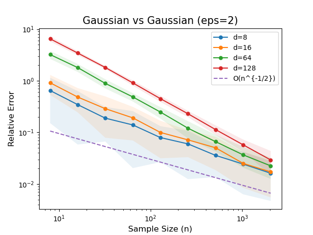
(b)

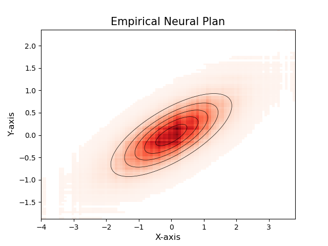
(c)

Figure 1. Neural Estimation of EGW alignment: (a) Relative error for the case where $\mu=\nu=\mathrm{Unif}\big{(}[-1/\sqrt{d},1/\sqrt{d}]^{d}\big{)}$; (b) Relative error for $\mu,\nu$ as centered Gaussian distributions with randomly generated covariance matrices; (c) Learned neural alignment plan (in red) versus the true optimal GW alignment (whose density is represented by the back contour lines).

We test our neural estimator on synthetic data, by estimating the EGW cost and alignment plan between uniform and Gaussian distribution in different dimensions. We consider dimensions $d\in\{8,16,64,128\}$, and for each $d$, employ a ReLU network of size $k\in\{32,64,128,256\}$, respectively. Accuracy is measured using the relative error $\big{|}\widehat{\mathrm{S}}_{k,a}^{\varepsilon}\left(X^{n},Y^{n}\right)-\widetilde{\mathsf{S}}^{\varepsilon}(\mu,\nu)\big{|}/\,\widetilde{\mathsf{S}}^{\varepsilon}(\mu,\nu)$, where $\widetilde{\mathsf{S}}^{\varepsilon}(\mu,\nu)$ is regarded as the group truth, which we obtain by running [SPC22, Algorithm 2] with $n=10,000$ samples (which we treat as $n\to\infty$ as it is $\times 5$ more than the largest sample set we use for our neural estimator). Each of the presented plots is averaged over 20 runs.

We first consider the EGW distance with $\varepsilon=0.5$ between two uniform distribution over a hypercube, namely, $\mu=\nu=\mathrm{Unif}\big{(}[-1/\sqrt{d},1/\sqrt{d}]^{d}\big{)}$. Fig. 1(a) plots the EGW neural estimation error versus the sample size $n\in\{8,16,32,64,128,256,512,1024,2048\}$ in a log-log scale. The curves exhibit a slope of approximately $-1/2$ for all dimensions, which validates our theory. In this experiment, we use an epoch number of 5, and set the stopping condition for updating $\mathbf{A}$ as either reaching a maximal iteration count of 100 or the Frobenius norm of gradient approximation dropping below $10^{-4}$.

Next, we test the EGW NE on unbounded measures. To that end, we set $\varepsilon=2$ and take $\mu,\nu$ as centered $d$-dimensional Gaussian distributions with randomly generated covariance matrices. Specifically, the two covariance matrices are of the form $\mathbf{B}^{\intercal}\mathbf{B}+1/(3d)\mathbf{I}_{d}$, where $\mathbf{I}_{d}$ is a $d\times d$ identity and $\mathbf{B}$ is a matrix whose entries are randomly sampled from $\mathrm{Unif}([-1/d,1/d])$. Note that the generated covariance matrix is positive semi-definite with eigenvalues set to lie in $[\frac{1}{3d},\frac{1}{d}]$. Fig. 1(b) plots the relative EGW neural estimation error for this Gaussian setting, again showing a parametric convergence rate. This experiment uses 10 epochs for the NE training, and the stopping condition for updating $\mathbf{A}$ is either reaching 200 iterations or that the Frobenius norm of gradient approximation drops below $10^{-3}$.

Lastly, we assess the quality of the neural alignment plan learned from our NE. Since doing so requires knowledge of the true (population) alignment plan $\pi^{\varepsilon}_{\star}$, we consider the IEGW distance $\mathsf{F}^{\varepsilon}$ (i.e., with inner product cost; see (12)) between Gaussians, for which a closed form expression for the optimal plan was derived in [LLN⁺22]. Adapting Algorithm 1 (which treats EGW with quadratic cost) to the IEGW case merely amounts to changing the constants in the approximate gradient formula from the expression in (21) to $16\mathbf{A}-8\sum_{1\leq i,j\leq n}X_{i}Y_{j}^{\intercal}\big{[}\widetilde{\bm{\Pi}}^{\varepsilon}_{\mathbf{A}}\big{]}_{ij}$, where $\widetilde{\bm{\Pi}}^{\varepsilon}_{\mathbf{A}}$ is now the optimal coupling for the EOT problem with the cost function $(x,y)\mapsto-8x^{\intercal}\mathbf{A}y$ (see Appendix A for more details on the IEGW setting). We take $\varepsilon=0.5$, $\mu=\mathcal{N}\left(0,1\right)$, and $\nu=\mathcal{N}(0,1/4)$. By Theorem 3.1 of [LLN⁺22], we have that $\pi^{\varepsilon}_{\star}=\mathcal{N}\left(\mathbf{0},\Sigma_{\star}\right)$ with

$$\Sigma_{\star}=\left(\begin{array}[]{cc}1&\frac{1}{\sqrt{8}}\\ \frac{1}{\sqrt{8}}&\frac{1}{4}\end{array}\right)$$

Figure 1(c) compares the neural coupling learned from our algorithm, shown in red, to the optimal $\pi^{\varepsilon}_{\star}$ given above, whose density is represented by the black contour line. The neural coupling is learned using $n=10^{4}$ samples and is realized by a NN with $k=40$ neurons. There is a clear correspondence between the two, which supports the result of Theorem 3.

4.3. MNIST Dataset

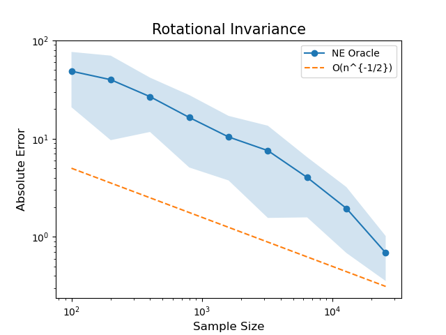
(a)

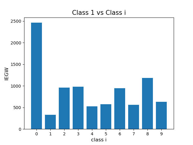
(b)

Figure 2. Neural Estimation of IEGW on MNIST: (a) Testing for the orthogonal invariance of the IEGW distance by estimating the gap $\big{|}\mathsf{F}^{\varepsilon}(\mu,\mu)-\mathsf{F}^{\varepsilon}(\mathbf{U}_{\sharp}\mu,\mathbf{V}_{\sharp}\mu)\big{|}$, for $\mu$ as the empirical MNIST distribution and $(\mathbf{U},\mathbf{V})$ two orthogonal matrices; (b) Capturing visual similarities between digits by estimating the IEGW distance between different MNIST digits.

We next test our NE on the MNIST dataset, as a simple example of real-world data. We again consider the IEGW distance $\mathsf{F}^{\varepsilon}$ for these experiments, due to the improved numerical stability it provides. We also set $\varepsilon$ to be large enough so that the algorithms does not incur numerical errors. To that end, we initiate a small $\varepsilon$ value, and if errors occur, double it until the algorithm converges without errors (eventually, we ended up using $\varepsilon=10^{3}$, which is an order of magnitude smaller than the threshold for convexity condition from [RGK23, Theorem 2] to hold).

We consider two experiments under the MNIST setting, one quantitative and another qualitative. For the first, we numerically test for the rotation invariance of the IEGW distance. Denoting the empirical distribution of the MNIST dataset by $\mu\in\mathcal{P}(\mathbb{R}^{784})$, for any two orthogonal matrices $\mathbf{U},\mathbf{V}$, we have $\mathsf{F}^{\varepsilon}(\mu,\mu)=\mathsf{F}^{\varepsilon}(\mathbf{U}_{\sharp}\mu,\mathbf{V}_{\sharp}\mu)$. Thus, we estimate the difference between these two quantities and evaluate its gap from 0, which is the ground truth. Specifically, we randomly sample data $(X_{0}^{n},X_{1}^{n})$ from $\mu\otimes\mu$, and $(Y_{0}^{n},Y_{1}^{n})$ from $(\mathbf{U},\mathbf{V})_{\sharp}\mu\otimes\mu$, with sample size $n\in\{100,200,400,800,1600,3200,6400,12800,25600\}$, and compute $\big{|}\mathsf{F}^{\varepsilon}_{k,a}(X_{0}^{n},X_{1}^{n})-\mathsf{F}^{\varepsilon}_{k,a}(Y_{0}^{n},Y_{1}^{n})\big{|}$ with $k=256$.

Fig. 2 plots the estimation error (averaged over 10 runs), decreasing from 48 to 0.68, which again exhibits a parametric rate of convergence, as expected. At $n=25600$, the absolute error of about $0.6$ amounts to $10^{-3}$ relative error (compared to the value of the NE, which is around 512). Notably, despite the data dimension being relatively large in this experiment, the NE successfully retrieves the correct value with moderate sample sizes. We have also attempted replicating this experiment using the Sinkhorn-based oracle from [RGK23, Algorithm 2], but the run time was prohibitively long for the larger $n$ values considered.

Lastly, we examine the ability of the IEGW NE to capture qualitative visual similarities between different digits in the MNIST dataset. To that end, we perform neural estimation of the IEGW distance between Class 1 and the other MNIST Classes, expecting, for example, a greater similarity (viz. smaller IEGW value) with digits like 4 and 7, but less so with 0, 3, and 8. The obtained estimates are plotted in Fig. 2(b), where the expected qualitative behavior is indeed observed.

5. Proofs

We first introduce a technical result from approximation theory that will be used in the subsequent derivations. The following result, which is a restatement of Proposition 10 from [SG22], states that a sufficiently smooth function over a compact domain can be approximated to within $O(k^{-1/2})$ error by a shallow NN.

Proposition 1 (Approximation of smooth functions; Proposition 10 from [SG22]).

Let $\mathcal{X}\subseteq\mathbb{R}^{d}$ be compact and $g:\mathcal{X}\rightarrow\mathbb{R}$. Suppose that there exists an open set $\mathcal{U}\supset\mathcal{X}$, $b\geq 0$, and $\tilde{g}\in\mathcal{C}_{b}^{s_{\mathsf{KB}}}(\mathcal{U})$, $s_{\mathsf{KB}}\coloneqq\lfloor d/2\rfloor+3$, such that $g=\tilde{g}\big{|}_{\mathcal{X}}$. Then, there exists $f\in\mathcal{F}_{k,d_{x}}\left(\bar{c}_{b,d,\|\mathcal{X}\|}\right)$, where $\bar{c}_{b,d,\|\mathcal{X}\|}$ is given in Equation (A.15) of [SG22], such that

$$\|f-g\|_{\infty}\lesssim\bar{c}_{b,d,\|\mathcal{X}\|}d^{\frac{1}{2}}k^{-\frac{1}{2}}.$$

This proposition will allow us to control the approximation error of the EGW NE. To invoke it, we will establish smoothness of the semi-dual EOT potentials arising in the variational representation from (11) (see Lemma 2 ahead). The smoothness of potentials stems from the presence of the entropic penalty and the smoothness of the cost function $c_{\mathbf{A}}$.

5.1. Proof of Theorem 1

For $(\mu,\nu)\in\mathcal{P}(\mathcal{X})\times\mathcal{P}(\mathcal{Y})$, define the population-level neural EOT cost as

$$\mathsf{OT}^{\varepsilon}_{c,k,a}(\mu,\nu)\coloneqq\sup_{f\in\mathcal{F}_{k,d}(a)}\int fd\mu+\int f^{c,\varepsilon}d\nu.$$ (23)

Having that, the population-level neural EGW cost is now given by

$$\mathsf{S}^{\varepsilon}_{k,a}(\mu,\nu)\coloneqq\mathsf{C}(\mu,\nu)+\inf_{\mathbf{A}\in\mathcal{D}_{M}}\Big{\{}32\|\mathbf{A}\|_{\mathrm{F}}^{2}+\mathsf{OT}^{\varepsilon}_{\mathbf{A},k,a}(\mu,\nu)\Big{\}},$$

where we have used the shorthand $\mathsf{OT}^{\varepsilon}_{\mathbf{A},k,a}(\mu,\nu)=\mathsf{OT}^{\varepsilon}_{c_{\mathbf{A}},k,a}(\mu,\nu)$. We decompose the neural estimation error into the approximation and empirical estimation errors:

$$\mathbb{E}\left[\left|\widehat{\mathsf{S}}_{k,a}^{\mspace{1.0mu}\varepsilon}\left(X^{n},Y^{n}\right)-\mathsf{S}^{\varepsilon}(\mu,\nu)\right|\right]$$ (24)

$$\leq\left|\mathsf{S}_{k,a}^{\mspace{1.0mu}\varepsilon}(\mu,\nu)-\mathsf{S}^{\varepsilon}(\mu,\nu)\right|+\mathbb{E}\left[\left|\mathsf{S}^{\varepsilon}_{k,a}(\mu,\nu)-\widehat{\mathsf{S}}^{\varepsilon}_{k,a}\left(X^{n},Y^{n}\right)\right|\right]$$

$$\leq\underbrace{\sup_{\mathbf{A}\in\mathcal{D}_{M}}\left|\mathsf{OT}^{\varepsilon}_{\mathbf{A},k,a}(\mu,\nu)-\mathsf{OT}^{\varepsilon}_{\mathbf{A}}(\mu,\nu)\right|}_{\text{Approximation error}}+\underbrace{\mathbb{E}\left[\left|\mathsf{C}(\mu,\nu)-\mathsf{C}\left(X^{n},Y^{n}\right)\right|\right]}_{\text{Estimation error 1}}$$

$$\qquad\qquad\qquad\qquad\qquad\qquad\qquad\qquad+\underbrace{\mathbb{E}\left[\sup_{\mathbf{A}\in\mathcal{D}_{M}}\left|\mathsf{OT}^{\varepsilon}_{\mathbf{A},k,a}(\mu,\nu)-\widehat{\mathsf{OT}}^{\varepsilon}_{\mathbf{A},k,a}\left(X^{n},Y^{n}\right)\right|\right]}_{\text{Estimation error 2}},$$ (25)

and analyze each term separately.

Approximation error. Proposition 1 provides a sup-norm approximation error bound of a smooth function by a NN. To invoke it, we first study the semi-dual EOT potentials and show that they are indeed smooth functions, i.e., admit an extension to an open set with sufficiently many bounded derivatives. The following lemma establishes regularity of semi-dual potentials for $\mathsf{OT}^{\varepsilon}_{\mathbf{A}}(\mu,\nu)$, uniformly in $\mathbf{A}\in\mathcal{D}_{M}$; afte stating it we shall account for the extension.

Lemma 2 (Uniform regularity of EOT potentials).

For any $\mathbf{A}\in\mathcal{D}_{M}$, there exist semi-dual EOT potentials $(\varphi_{\mathbf{A}},\varphi^{c,\varepsilon}_{\mathbf{A}})$ for $\mathsf{OT}_{\mathbf{A}}^{\mspace{1.0mu}\varepsilon}(\mu,\nu)$, such that

$$\|\varphi_{\mathbf{A}}\|_{\infty,\mathcal{X}} \leq 6d_{x}d_{y}+40(d_{x}d_{y})^{3/2}$$ (26)

$$\left\|D^{\alpha}\varphi_{\mathbf{A}}\right\|_{\infty,\mathcal{X}} \leq C_{s}\left(1+\varepsilon^{1-s}\right)\left(1+d_{y}\right)^{s}\left(1+\sqrt{d_{x}}d_{y}+\sqrt{d_{x}}\right)^{s},\quad\forall\alpha\in\mathbb{N}_{0}^{d_{x}}\text{ with }1\leq|\alpha|\leq s,$$

for any $s\geq 2$ and some constant $C_{s}$ that depends only on $s$. Analogous bounds hold for $\varphi_{\mathbf{A}}^{c,\varepsilon}$.

The lemma is proven in Section B.1. The derivation is similar to that of Lemma 4 in [ZGMS22], but the bounds are adapted to the compactly supported case and present an explicit dependence on $\varepsilon$ (as opposed to the $\varepsilon=1$ assumption that was imposed in that work).

Let $(\varphi_{\mathbf{A}},\varphi^{c,\varepsilon}_{\mathbf{A}})$ be semi-dual potentials as in Lemma 2 (i.e., satisfying (26)) with the normalization $\int\varphi_{\mathbf{A}}d\mu=\int\varphi^{c,\varepsilon}_{\mathbf{A}}d\nu=\frac{1}{2}\mathrm{OT}_{\mathbf{A}}^{\varepsilon}(\mu,\nu)$. Define the natural extension of $\varphi_{\mathbf{A}}$ to the open ball of radius $\sqrt{2d_{x}}$:

$$\tilde{\varphi}_{\mathbf{A}}(x)\coloneqq-\varepsilon\log\int_{\mathcal{Y}}\exp\left(\frac{\psi_{\mathbf{A}}(y)-c_{\mathbf{A}}(x,y)}{\varepsilon}\right)d\nu(y),\quad x\in B_{d_{x}}(\sqrt{2d_{x}}),$$

and notice that $\tilde{\varphi}_{\mathbf{A}}\big{|}_{\mathcal{X}}=\varphi_{\mathbf{A}}$, pointwise on $\mathcal{X}$. Similarly, consider its $(c,\varepsilon)$-transform $\tilde{\varphi}_{\mathbf{A}}^{c,\varepsilon}$ extended to $B_{d_{y}}(\sqrt{2d_{y}})$, and again observe that $\tilde{\varphi}_{\mathbf{A}}^{c,\varepsilon}\big{|}_{\mathcal{Y}}=\varphi_{\mathbf{A}}^{c,\varepsilon}$. Following the proof of Lemma 2, one readily verifies that for any $s\geq 2$, we have

$$\|\tilde{\varphi}_{\mathbf{A}}\|_{\infty,B_{d_{x}}\left(\sqrt{2d_{x}}\right)} \leq 10d_{x}d_{y}+(24+16\sqrt{2})(d_{x}d_{y})^{3/2}$$ (27)

$$\left\|D^{\alpha}\tilde{\varphi}_{\mathbf{A}}\right\|_{\infty,B_{d_{x}}\left(\sqrt{2d_{x}}\right)} \leq C_{s}\left(1+\varepsilon^{1-s}\right)\left(1+d_{y}\right)^{s}\left(1+\sqrt{d_{x}}d_{y}+\sqrt{d_{x}}\right)^{s},\forall\alpha\in\mathbb{N}_{0}^{d_{x}},\ 1\leq|\alpha|\leq s.$$

Recall that $s_{\mathsf{KB}}=\left\lfloor d_{x}/2\right\rfloor+3$ and set

$$C_{d_{x},d_{y}}\coloneqq\left\{\left(1+d_{y}\right)^{s_{\mathsf{KB}}}\left(1+\sqrt{d_{x}}d_{y}+\sqrt{d_{x}}\right)^{s_{\mathsf{KB}}}\right\}\vee\left\{10d_{x}d_{y}+(24+16\sqrt{2})(d_{x}d_{y})^{3/2}\right\}.$$ (28)

By (27), we now have

$$\max_{\alpha:\,|\alpha|\leq s_{\mathsf{KB}}}\left\|D^{\alpha}\tilde{\varphi}_{\mathbf{A}}\right\|_{\infty,B_{d_{x}}\left(\sqrt{2d_{x}}\right)}\leq C_{s_{\mathsf{KB}}}C_{d_{x},d_{y}}(1+\varepsilon^{1-s_{\mathsf{KB}}})\coloneqq b,$$ (29)

and so $\tilde{\varphi}_{\mathbf{A}}\in\mathcal{C}_{b}^{s_{\mathsf{KB}}}\big{(}B_{d_{x}}(\sqrt{2d_{x}})\big{)}$.

Noting that $\mathcal{X}\subset B_{d_{x}}(\sqrt{2d_{x}})$, by Proposition 1, there exists $f\in\mathcal{F}_{k,d_{x}}\left(\bar{c}_{b,d_{x}}\right)$ such that

$$\left\|\varphi_{\mathbf{A}}-f\right\|_{\infty,\mathcal{X}}\lesssim\bar{c}_{b,d_{x}}d^{\frac{1}{2}}k^{-\frac{1}{2}},$$ (30)

where $\bar{c}_{b,d_{x}}=b\,\bar{c}_{d_{x}}$ and $\bar{c}_{d_{x}}$ is defined as (see [SG22, Equation (A.15)])

$$\bar{c}_{d_{x}} \coloneqq\left(\kappa_{d_{x}}{d_{x}}^{\frac{3}{2}}\vee 1\right)\pi^{\frac{d_{x}}{2}}$$ (31)

$$\times\Gamma\left(\frac{d_{x}}{2}+1\right)^{-1}(\operatorname{rad}(\mathcal{X})+1)^{d_{x}}2^{s_{\mathsf{KB}}}d_{x}\left(\frac{1-{d_{x}}^{\frac{s_{\mathsf{KB}}}{2}}}{1-\sqrt{d_{x}}}+{d_{x}}^{\frac{s_{\mathsf{KB}}}{2}}\right)\max_{\|\alpha\|_{1}\leq s_{\mathsf{KB}}}\left\|D^{\alpha}\Psi\right\|_{\infty,B_{d}(0.5)},$$

with $\kappa_{d_{x}}^{2}\coloneqq\left(d_{x}+{d_{x}}^{(s_{\mathsf{KB}}-1)}\right)\int_{\mathbb{R}^{d}}\left(1+\|\omega\|^{2\left(s_{\mathsf{KB}}-2\right)}\right)^{-1}d\omega$, $\operatorname{rad}(\mathcal{X})=0.5\sup_{x,x^{\prime}\in\mathcal{X}}\left\|x-x^{\prime}\right\|$ and $\Psi(x)\propto\exp\left(-\frac{1}{0.5-\|x\|^{2}}\right)\mathbbm{1}_{\{\|x\|<0.5\}}$ as the canonical mollifier normalized to have unit mass.

Our last step is to lift the sup-norm neural approximation bound on the semi-dual potential from (30) to a bound on the approximation error of the corresponding EOT cost. The following lemma is proven in Section B.2.

Lemma 3 (Neural approximation error reduction).

Fix $(\mu,\nu)\in\mathcal{P}(\mathcal{X})\times\mathcal{P}(\mathcal{Y})$ and let $\varphi_{\mathbf{A}}$ be the semi-dual EOT potential for $\mathsf{OT}^{\varepsilon}_{\mathbf{A}}(\mu,\nu)$ from Lemma 2. For any $f\in\mathcal{F}_{k,d_{x}}\left(a\right)$, we have

$$\left|\mathsf{OT}^{\varepsilon}_{\mathbf{A}}(\mu,\nu)-\mathsf{OT}^{\varepsilon}_{\mathbf{A},k,a}(\mu,\nu)\right|\leq 2\left\|\varphi_{\mathbf{A}}-f\right\|_{\infty,\mathcal{X}}.$$

Setting $a=\bar{c}_{b,d_{x}}$ and combining Lemma 3 with (30), we obtain

$$\left|\mathsf{OT}^{\varepsilon}_{\mathbf{A},k,a}(\mu,\nu)-\mathsf{OT}^{\varepsilon}_{\mathbf{A}}(\mu,\nu)\right|\leq 2\bar{c}_{b,d_{x}}k^{-\frac{1}{2}}.$$

As the RHS above is independent of $\mathbf{A}\in\mathcal{D}_{M}$, we conclude that

$$\sup_{\mathbf{A}\in\mathcal{D}_{M}}\left|\mathsf{OT}^{\varepsilon}_{\mathbf{A},k,a}(\mu,\nu)-\mathsf{OT}^{\varepsilon}_{\mathbf{A}}(\mu,\nu)\right|\lesssim_{d_{x},d_{y}}\left(1+\frac{1}{\varepsilon^{\left\lfloor\frac{d_{x}}{2}\right\rfloor+2}}\right)k^{-\frac{1}{2}}.$$ (32)

Estimation error 1. The estimation rate for $\mathsf{C}(\mu,\nu)$ was derived as part of the proof of [ZGMS22, Theorem 2] under a 4-sub-Weibull assumption on the population distributions. Since our $\mu,\nu$ are compactly supported, they are also 4-sub-Weilbull with parameter $\sigma^{2}=\frac{(d_{x}\vee d_{y})^{2}}{2\ln 2}$, and we consequently obtain

$$\mathbb{E}\left[\left|\mathsf{C}(\mu,\nu)-\mathsf{C}\left(X^{n},Y^{n}\right)\right|\right]\lesssim\frac{1+\sigma^{4}}{\sqrt{n}}.$$ (33)

Estimation error 2. Set $\mathcal{F}^{c,\varepsilon}(a)\coloneqq\bigcup_{\mathbf{A}\in\mathcal{D}_{M}}\left\{f^{c_{\mathbf{A}},\varepsilon}:f\in\mathcal{F}_{k,d_{x}}(a)\right\}$, and first bound

$$\mathbb{E}\left[\sup_{\mathbf{A}\in\mathcal{D}_{M}}\left|\mathsf{OT}^{\varepsilon}_{\mathbf{A},k,a}(\mu,\nu)-\widehat{\mathsf{OT}}^{\varepsilon}_{\mathbf{A},k,a}\left(X^{n},Y^{n}\right)\right|\right]$$

$$\leq\underbrace{n^{-\frac{1}{2}}\mathbb{E}\left[\sup_{f\in\mathcal{F}_{k,d_{x}}(a)}\mspace{-3.0mu}n^{-\frac{1}{2}}\left|\sum_{i=1}^{n}\big{(}f(X_{i})-\mathbb{E}_{\mu}[f]\big{)}\right|\right]}_{(\mathrm{I})}+\mspace{-2.0mu}\underbrace{n^{-\frac{1}{2}}\mathbb{E}\left[\sup_{f\in\mathcal{F}^{c,\varepsilon}(a)}\mspace{-3.0mu}n^{-\frac{1}{2}}\left|\sum_{j=1}^{n}\big{(}f(Y_{j})-\mathbb{E}_{\nu}[f]\big{)}\right|\right]}_{(\mathrm{II})}.$$ (34)

To control these expected suprema, we again require regularity of the involved function, as stated in the next lemma.

Lemma 4.

Fix $c\in\mathcal{C}^{\infty}$, the $(c,\varepsilon)$-transform of NNs class $\mathcal{F}_{k,d_{x}}(a)$ satisfies the following uniform smoothness properties:

$$\|f^{c,\varepsilon}\|_{\infty,\mathcal{Y}} \leq\|c\|_{\infty,\mathcal{X}\times\mathcal{Y}}+3a(\|\mathcal{X}\|+1)$$ (35)

$$\left\|D^{\alpha}f^{c,\varepsilon}\right\|_{\infty,\mathcal{Y}} \leq C_{s}C_{c,\|\mathcal{X}\|,\|\mathcal{Y}\|}\left(1+\varepsilon^{1-s}\right)\quad,\forall\alpha\in\mathbb{N}_{0}^{d_{x}}\text{ with }1\leq|\alpha|\leq s$$

for any $s\geq 2$ and $f\in\mathcal{F}_{k,d_{x}}(a)$. In particular, taking $c=c_{\mathbf{A}}$, for any $\mathbf{A}\in\mathcal{D}_{M}$, there exists a constant $R_{s}$ that depends only on $s,d_{x},d_{y}$, such that

$$\max_{\alpha:|\alpha|_{1}\leq s}\left\|D^{\alpha}f^{c_{\mathbf{A}},\varepsilon}\right\|_{\infty,\mathcal{Y}}\leq R_{s}(1+a)(1+\varepsilon^{1-s})$$

for any $s\geq 2$ and $f\in\mathcal{F}_{k,d_{x}}(a)$.

The only difference between Lemmas 2 and 4 is that here we consider the $(c,\varepsilon)$-transform of NNs, rather than of dual EOT potentials. As our NNs are also compactly supported and bounded, the derivation of this result is all but identical to the proof of Lemma 2, and is therefore omitted to avoid repetition.

We proceed to bound Terms $(\mathrm{I})$ and $(\mathrm{II})$ from (5.1). For the first, consider

$$\mathbb{E}\left[\sup_{f\in\mathcal{F}_{k,d_{x}}(a)}n^{-\frac{1}{2}}\left|\sum_{i=1}^{n}\left(f(X_{i})-\mathbb{E}_{\mu}[f]\right)\right|\right] \stackrel{{\scriptstyle(a)}}{{\lesssim}}\mathbb{E}\left[\int_{0}^{\infty}\sqrt{\log N\left(\delta,\mathcal{F}_{k,d_{x}}(a),\|\cdot\|_{2,\mu_{n}}\right)}d\delta\right]$$

$$\leq\int_{0}^{\infty}\sqrt{\sup_{\gamma\in\mathcal{P}(\mathcal{X})}\log N\left(\delta,\mathcal{F}_{k,d_{x}}(a),\|\cdot\|_{2,\gamma}\right)}d\delta$$

$$\stackrel{{\scriptstyle(b)}}{{=}}\int_{0}^{12a}\sqrt{\sup_{\gamma\in\mathcal{P}(\mathcal{X})}\log N\left(\delta,\mathcal{F}_{k,d_{x}}(a),\|\cdot\|_{2,\gamma}\right)}d\delta$$

$$\lesssim a\int_{0}^{1}\sqrt{\sup_{\gamma\in\mathcal{P}(\mathcal{X})}\log N\left(6a\delta,\mathcal{F}_{k,d_{x}}(a),\|\cdot\|_{2,\gamma}\right)}d\delta$$

$$\stackrel{{\scriptstyle(c)}}{{\lesssim}}ad_{x}^{\frac{3}{2}},$$ (36)

where:

(a) follows by [vdVW96, Corollary 2.2.8] since $n^{-\frac{1}{2}}\sum_{i=1}^{n}\sigma_{i}f\left(X_{i}\right)$, where $\{\sigma_{i}\}_{i=1}^{n}$ are i.i.d Rademacher random variables, is sub-Gaussian w.r.t. pseudo-metric $\|\cdot\|_{2,\mu_{n}}$ (by Hoeffding’s inequality) ;

(b) is since $\bar{C}\left(\left|\mathcal{F}_{k,d_{x}}(a)\right|,\mathcal{X}\right)\leq 3a(\|\mathcal{X}\|+1)=6a$ and $N\left(\delta,\mathcal{F}_{k,d_{x}}(a),\|\cdot\|_{2,\gamma}\right)=1$, whenever $\delta>12a$;

(c) uses the bound $\int_{0}^{1}\sqrt{\sup_{\gamma\in\mathcal{P}(\mathcal{X})}\log N\left(6a\delta,\mathcal{F}_{k,d_{x}}(a),\|\cdot\|_{2,\gamma}\right)}d\delta\lesssim d_{x}^{\frac{3}{2}}$, which follows from step (A.33) in [SG22].

For Term $(\mathrm{II})$, let $s=\left\lceil d_{y}/2\right\rceil+1$, and consider

$$\mathbb{E}\left[\sup_{f\in\mathcal{F}^{c,\varepsilon}(a)}n^{-\frac{1}{2}}\left|\sum_{i=1}^{n}\big{(}f\left(Y_{i}\right)-\mathbb{E}_{\mu}[f]\big{)}\right|\right] \stackrel{{\scriptstyle(a)}}{{\lesssim}}\int_{0}^{12a}\sqrt{\sup_{\gamma\in\mathcal{P}(\mathcal{Y})}\log N\left(\delta,\mathcal{F}^{c,\varepsilon}(a),\|\cdot\|_{2,\gamma}\right)}d\delta$$

$$\lesssim\int_{0}^{12a}\sqrt{\sup_{\gamma\in\mathcal{P}(\mathcal{Y})}\log N_{[\,]}\left(2\delta,\mathcal{F}^{c,\varepsilon}(a),\|\cdot\|_{2,\gamma}\right)}d\delta$$

$$\stackrel{{\scriptstyle(b)}}{{\lesssim}}K_{s}\int_{0}^{12a}\left(\frac{R_{s}(1+a)(1+\varepsilon^{1-s})}{2\delta}\right)^{\frac{d_{y}}{2s}}d\delta$$

$$\lesssim_{c,d_{x},d_{y}}a(1+a)(1+\varepsilon^{1-s}),$$ (37)

where $R_{s}$ is the constant from Lemma 4 (which depends only $s,d_{x},d_{y}$), (a) follows by a similar argument to that from the bound on Term $(\mathrm{I})$, along with equation (50), which specifies the upper limit for entropy integral, while (b) follows by Lemma 4 and [vdVW96, Corollary 2.7.2], which upper bounds the bracketing entropy number of smooth functions on a bounded convex support.

To arrive at the effective error bound from Theorem 1, we provide a second bound on Term $(\mathrm{II})$. This second bound yields a better dependence on dimension (namely, only the smaller dimension $d_{x}$ appears in the exponent) at the price of another $\sqrt{k}$ factor. Neither bound is uniformly superior over the other, and hence our final result will simply take the minimum of the two. By (50) from the proof of Lemma 3, we have

$$N\left(\delta,\mathcal{F}^{c,\varepsilon}(a),\|\cdot\|_{2,\gamma}\right)\leq N\left(\delta,\mathcal{F}_{k,d_{x}}(a),\|\cdot\|_{\infty,\mathcal{X}}\right).$$

Invoking Lemma 2 from [SG22], which upper bounds the metric entropy of ReLU NNs class on the RHS above, we further obtain

$$\log N\left(\delta,\mathcal{F}_{k,d_{x}}(a),\|\cdot\|_{\infty,\mathcal{X}}\right)\leq\big{(}(d_{x}+2)k+d_{x}+1\big{)}\log\left(1+20a(\|\mathcal{X}\|+1)\delta^{-1}\right),$$ (38)

and proceed to bound Term $(\mathrm{II})$ as follows:

$$\mathbb{E}\left[\sup_{f\in\mathcal{F}^{c,\varepsilon}}n^{-\frac{1}{2}}\left|\sum_{j=1}^{n}\big{(}f(Y_{j})-\mathbb{E}_{\nu}[f]\big{)}\right|\right] \lesssim a\int_{0}^{1}\sqrt{\sup_{\gamma\in\mathcal{P}(\mathcal{X})}\log N\left(6a\delta,\mathcal{F}^{c,\varepsilon}(a),\|\cdot\|_{2,\gamma}\right)}d\delta$$

$$\lesssim ad_{x}^{\frac{1}{2}}\sqrt{k}\int_{0}^{1}\sqrt{\log(1+7\delta^{-1})}d\delta$$

$$\lesssim ad_{x}^{\frac{1}{2}}\sqrt{k}.$$ (39)

Inserting (36), (37), and (39) back into (5.1), we obtain the desired bound on the empirical estimation error by setting $a=\bar{c}_{b,d_{x}}$, as was defined in approximation error analysis:

$$\mathbb{E} \left[\sup_{\mathbf{A}\in\mathcal{D}_{M}}\left|\mathsf{OT}^{\varepsilon}_{\mathbf{A},k,a}(\mu,\nu)-\widehat{\mathsf{OT}}^{\varepsilon}_{\mathbf{A},k,a}\left(X^{n},Y^{n}\right)\right|\right]$$ (40)

$$\qquad\qquad\qquad\qquad\qquad\qquad\lesssim_{d_{x},d_{y}}\min\left\{1+\frac{1}{\varepsilon^{\left\lceil d_{x}+\frac{d_{y}}{2}\right\rceil+4}}\,,\left(1+\frac{1}{\varepsilon^{\left\lfloor\frac{d_{x}}{2}\right\rfloor+2}}\right)\sqrt{k}\right\}n^{-\frac{1}{2}}.$$

The proof is concluded by plugging the approximation error bound from (32) and the two estimation error bounds from (33) and (40) into (25), and supremizing over $(\mu,\nu)\in\mathcal{P}(\mathcal{X})\times\mathcal{P}(\mathcal{Y})$, while noting that all the above bounds holds uniformly in the two distributions. ∎

5.2. Proof of Theorem 2

This proof is similar to that of Theorem 1, up to minor modifications. For brevity, we only highlight the required changes. Note that for $k$ with $m_{k}\geq\bar{c}_{b,d_{x}}$, where the latter is defined in proof of Theorem 1 (see (29) and (31)), we have $\mathcal{F}_{k,d_{x}}(\bar{c}_{b,d_{x}})\subset\mathcal{F}_{k,d_{x}}(m_{k})$. Hence, by Lemma 3 and (30), there exists a NN $f\in\mathcal{F}_{k,d_{x}}(\bar{c}_{b,d_{x}})$, such that

$$\left|\mathsf{OT}^{\varepsilon}_{\mathbf{A}}(\mu,\nu)-\mathsf{OT}^{\varepsilon}_{\mathbf{A},k,m_{k}}(\mu,\nu)\right|\leq 2\left\|\varphi_{\mathbf{A}}-f\right\|_{\infty,\mathcal{X}}\lesssim_{d_{x},d_{y}}\left(1+\frac{1}{\varepsilon^{\left\lfloor\frac{d_{x}}{2}\right\rfloor+2}}\right)k^{-\frac{1}{2}}.$$

Next, for estimation error, by setting $a=m_{k}\coloneqq\log k\vee 1$ in (36), (37), and (39) (instead of $a=\bar{c}_{b,d_{x}}$ as in the proof of Theorem 1), we arrive at

$$\mathbb{E}\left[\sup_{\mathbf{A}\in\mathcal{D}_{M}}\left|\mathsf{OT}^{\varepsilon}_{\mathbf{A},k,m_{k}}(\mu,\nu)-\widehat{\mathsf{OT}}^{\varepsilon}_{\mathbf{A},k,m_{k}}\left(X^{n},Y^{n}\right)\right|\right]$$

$$\qquad\qquad\qquad\qquad\qquad\qquad\qquad\qquad\lesssim_{d_{x},d_{y}}\min\left\{\left(1+\frac{1}{\varepsilon^{\left[\frac{d_{y}}{2}\right\rceil}}\right)(\log k)^{2}\,,\sqrt{k}\log k\right\}n^{-\frac{1}{2}}.$$

Combining this with the sample complexity of estimating $\mathsf{C}(\mu,\nu)$ given in (33), we conclude

$$\sup_{(\mu,\nu)\in\mathcal{P}(\mathcal{X})\times\mathcal{P}(\mathcal{Y})}\mspace{-5.0mu}\mathbb{E}\left[\left|\widehat{\mathsf{S}}_{k,m_{k}}^{\mspace{1.0mu}\varepsilon}(X^{n},Y^{n})\mspace{-2.0mu}-\mspace{-2.0mu}\mathsf{S}^{\varepsilon}(\mu,\nu)\right|\right]$$

$$\qquad\qquad\qquad\lesssim_{d_{x},d_{y}}\left(1+\frac{1}{\varepsilon^{\left\lfloor\frac{d_{x}}{2}\right\rfloor+2}}\right)k^{-\frac{1}{2}}+\min\left\{\left(1+\frac{1}{\varepsilon^{\left[\frac{d_{y}}{2}\right\rceil}}\right)(\log k)^{2}\,,\sqrt{k}\log k\right\}n^{-\frac{1}{2}}.$$

∎

5.3. Proof of Theorem 3

Fix $\mathbf{A}\in\mathcal{D}_{M}$. Define $\Gamma_{\mathbf{A}}(f):=\int_{\mathcal{X}}fd\mu+\int_{\mathcal{Y}}f^{c_{\mathbf{A}},\varepsilon}d\nu$, and let $\varphi_{\mathbf{A}}$ be optimal potential of $\mathsf{OT}_{{\mathbf{A}}}^{\varepsilon}(\mu,\nu)$, solving semi-dual formulation. Denote the corresponding optimal coupling by $\pi^{\varepsilon}_{\mathbf{A}}$. We first show that for any continuous $f:\mathcal{X}\to\mathbb{R}$, the following holds:

$$\Gamma_{\mathbf{A}}\left(\varphi_{\mathbf{A}}\right)-\Gamma_{\mathbf{A}}\left(f\right)=\varepsilon\mathsf{D}_{\mathsf{KL}}\big{(}\pi^{\varepsilon}_{\mathbf{A}}\big{\|}\pi^{\varepsilon}_{\mathbf{A},f}\big{)},$$ (41)

where (see (16))

$$d\pi^{\varepsilon}_{\mathbf{A},f}(x,y)=\frac{\exp\left(\frac{f(x)-c_{\mathbf{A}}(x,y)}{\varepsilon}\right)}{\int_{\mathcal{X}}\exp\left(\frac{f-c_{\mathbf{A}}(\cdot,y)}{\varepsilon}\right)d\mu}d\mu\otimes\nu(x,y).$$

The derivation is inspired by the proof of [MKB23, Theorem 2], with several technical modifications. Since $\mu\in\mathcal{P}_{\mathsf{ac}}(\mathcal{X})$ with Lebesgue density $\frac{d\mu}{dx}$, define its energy function $E_{\mu}:\mathcal{X}\rightarrow\mathbb{R}$ by $\frac{d\mu(x)}{dx}\propto\exp\left(-E_{\mu}(x)\right)$. Also define conditional distribution $d\pi^{\varepsilon}_{\mathbf{A},f}(\cdot|y)\coloneqq\frac{d\pi_{\mathbf{A},f}(\cdot,y)}{d\nu(y)}$, and set $\tilde{f}\coloneqq f-\varepsilon E_{\mu}(x)$. We have

$$\frac{d\pi^{\varepsilon}_{\mathbf{A},f}(x|y)}{dx}=\frac{d\pi^{\varepsilon}_{\mathbf{A},f}(x,y)}{d\nu(y)dx}\mspace{-0.5mu}=\mspace{-0.5mu}\frac{\exp\left(\frac{f(x)-c_{\mathbf{A}}(x,y)}{\varepsilon}\right)\frac{d\mu(x)}{dx}}{\int_{\mathcal{X}}\exp\left(\frac{f(x^{\prime})-c_{\mathbf{A}}(x^{\prime},y)}{\varepsilon}\right)\frac{d\mu}{dx^{\prime}}(x^{\prime})dx^{\prime}}\mspace{-0.5mu}=\mspace{-0.5mu}\frac{\exp\left(\frac{\tilde{f}(x)-c_{\mathbf{A}}(x,y)}{\varepsilon}\right)}{\int_{\mathcal{X}}\exp\left(\frac{\tilde{f}(x^{\prime})-c_{\mathbf{A}}(x^{\prime},y)}{\varepsilon}\right)dx^{\prime}}.$$

Define the shorthands $F_{f}(y)\coloneqq\int_{\mathcal{X}}\exp\left(\frac{f(x)-c_{\mathbf{A}}(x,y)}{\varepsilon}\right)dx$ and $Z\coloneqq\int_{\mathcal{X}}\exp\big{(}-E_{\mu}(x)\big{)}dx$, and note that the $(c,\varepsilon)$-transform of $f$ w.r.t. the cost function $c_{\mathbf{A}}$ can be expressed as

$$f^{c_{\mathbf{A}},\varepsilon}(y) =-\varepsilon\log\left(\int_{\mathcal{X}}\exp\left(\frac{f(x)-c_{\mathbf{A}}(x,y)}{\varepsilon}\right)\frac{d\mu(x)}{dx}dx\right)$$

$$=-\varepsilon\log\left(\int_{\mathcal{X}}\exp\left(\frac{\tilde{f}(x)-c_{\mathbf{A}}(x,y)}{\varepsilon}\right)dx\right)+\varepsilon\log(Z)$$

$$=-\varepsilon\log\big{(}F_{\tilde{f}}(y)\big{)}+\varepsilon\log(Z).$$

We are now ready to prove (41). For $\rho\in\mathcal{P}_{\mathsf{ac}}(\mathcal{X})$ with Lebesgue density $\frac{d\rho}{dx}$, denote the differential entropy of $\rho$ by $\mathsf{H}(\rho)\coloneqq-\int_{\mathcal{X}}\log\left(\frac{d\rho}{dx}\right)d\rho$. Consider:

$$\Gamma_{\mathbf{A}}\left(\varphi_{\mathbf{A}}\right)-\Gamma_{\mathbf{A}}\left(f\right)$$

$$=\int_{\mathcal{X}\times\mathcal{Y}}c_{\mathbf{A}}d\pi^{\varepsilon}_{\mathbf{A}}-\varepsilon\int_{\mathcal{Y}}\mathsf{H}\big{(}\pi^{\varepsilon}_{\mathbf{A}}(\cdot|y)\big{)}d\nu(y)+\varepsilon\mathsf{H}(\mu)-\int_{\mathcal{X}}fd\mu-\int_{\mathcal{Y}}f^{c_{\mathbf{A}},\varepsilon}d\nu$$

$$=\int_{\mathcal{X}\times\mathcal{Y}}\big{(}c_{\mathbf{A}}(x,y)-\tilde{f}(x)\big{)}d\pi^{\varepsilon}_{\mathbf{A}}(x,y)-\varepsilon\int_{\mathcal{Y}}\mathsf{H}\big{(}\pi^{\varepsilon}_{\mathbf{A}}(\cdot|y)\big{)}d\nu(y)+\varepsilon\int_{\mathcal{Y}}\log\big{(}F_{\tilde{f}}\big{)}d\nu$$

$$=-\varepsilon\int_{\mathcal{X}\times\mathcal{Y}}\frac{\tilde{f}(x)-c_{\mathbf{A}}(x,y)}{\varepsilon}d\pi^{\varepsilon}_{\mathbf{A}}(x,y)+\varepsilon\int_{\mathcal{X}\times\mathcal{Y}}\log\big{(}F_{\tilde{f}}(y)\big{)}d\pi_{\mathbf{A}}^{\varepsilon}(x,y)-\varepsilon\int_{\mathcal{Y}}\mathsf{H}\big{(}\pi_{\mathbf{A}}^{\varepsilon}(\cdot|y)\big{)}d\nu(y)$$

$$=-\varepsilon\int_{\mathcal{X}\times\mathcal{Y}}\log\left(\frac{1}{F_{\tilde{f}}(y)}\exp\left(\frac{\tilde{f}(x)-c_{\mathbf{A}}(x,y)}{\varepsilon}\right)\right)d\pi_{\mathbf{A}}^{\varepsilon}(x,y)-\varepsilon\int_{\mathcal{Y}}\mathsf{H}\big{(}\pi_{\mathbf{A}}^{\varepsilon}(\cdot|y)\big{)}d\nu(y)$$

$$=-\varepsilon\int_{\mathcal{X}\times\mathcal{Y}}\log\left(\frac{d\pi^{\varepsilon}_{\mathbf{A},f}(x\mid y)}{dx}\right)d\pi_{\mathbf{A}}^{\varepsilon}(x,y)-\varepsilon\int_{\mathcal{Y}}\mathsf{H}\big{(}\pi_{\mathbf{A}}^{\varepsilon}(\cdot|y)\big{)}d\nu(y)$$

$$=-\varepsilon\int_{\mathcal{Y}}\int_{\mathcal{X}}\log\left(\frac{d\pi^{\varepsilon}_{\mathbf{A},f}(x|y)}{dx}\right)d\pi_{\mathbf{A}}^{\varepsilon}(x|y)d\nu(y)+\varepsilon\int_{\mathcal{Y}}\int_{\mathcal{X}}\log\left(\frac{d\pi_{\mathbf{A}}^{\varepsilon}(x|y)}{dx}\right)d\pi_{\mathbf{A}}^{\varepsilon}(x|y)d\nu(y)$$

$$=\varepsilon\int_{\mathcal{Y}}\int_{\mathcal{X}}\log\left(\frac{d\pi_{\mathbf{A}}^{\varepsilon}(x|y)}{d\pi^{\varepsilon}_{\mathbf{A},f}(x|y)}\right)d\pi_{\mathbf{A}}^{\varepsilon}(x|y)d\nu(y)$$

$$=\varepsilon\int_{\mathcal{X}\times\mathcal{Y}}\log\left(\frac{d\pi_{\mathbf{A}}^{\varepsilon}(x,y)}{d\pi^{\varepsilon}_{\mathbf{A},f}(x,y)}\right)d\pi_{\mathbf{A}}^{\varepsilon}(x,y)$$

$$=\varepsilon\mathsf{D}_{\mathsf{KL}}\left(\pi_{\mathbf{A}}^{\varepsilon}\middle\|\pi^{\varepsilon}_{\mathbf{A},f}\right).$$

Since $\mathbf{A}_{\star}$ is a minimizer of (11), Corollary 1 from [RGK23] implies that $\pi^{\varepsilon}_{\mathbf{A}_{\star}}=\pi^{\varepsilon}_{\star}$, where the latter is an optimal EGW alignment plan (i.e., an optimizer of (9)). Recalling that $\hat{f}_{\star}$ is a NN that optimizes the NE $\widehat{\mathsf{OT}}^{\varepsilon}_{\mathbf{A}_{\star},k,a}(X^{n},Y^{n})$ from (14), and plugging it into (41) yields $\mathsf{D}_{\mathsf{KL}}\big{(}\pi^{\varepsilon}_{\star}\big{\|}\pi^{\varepsilon}_{\mathbf{A}_{\star},\hat{f}_{\star}}\big{)}=\varepsilon^{-1}\big{[}\Gamma_{\mathbf{A}_{\star}}\left(\varphi_{\mathbf{A}_{\star}}\right)-\Gamma_{\mathbf{A}_{\star}}(\hat{f}_{\star})\big{]}$. Thus, to prove the KL divergence bound from Theorem 3, it suffices to control the gap between the $\Gamma$ functionals on the RHS above.

Write $f_{\star}$ for a NN that maximizes the population-level neural EOT cost $\mathsf{OT}_{\mathbf{A}_{\star},k,a}^{\varepsilon}(\mu,\nu)$ (see (23)). Define $\widehat{\Gamma}_{\mathbf{A}}(f):=\frac{1}{n}\sum_{i=1}^{n}\big{[}f(X_{i})-f^{c_{\mathbf{A}},\varepsilon}(Y_{i})\big{]}$ for the optimization objective in the problem $\widehat{\mathsf{OT}}_{\mathbf{A},k,a}^{\varepsilon}(X^{n},Y^{n})$ (see (14)), and note that $\hat{f}_{\star}$ is a maximizer of $\widehat{\Gamma}_{\mathbf{A}_{\star}}$. We now have

$$\varepsilon\mathsf{D}_{\mathsf{KL}}\left(\pi_{\star}^{\varepsilon}\middle\|\pi^{\varepsilon}_{\mathbf{A}_{\star},\hat{f}_{\star}}\right)$$ (42)

$$=\Gamma_{\mathbf{A}_{\star}}\left(\varphi_{\mathbf{A}_{\star}}\right)-\Gamma_{\mathbf{A}_{\star}}\left(f_{\star}\right)+\Gamma_{\mathbf{A}_{\star}}\left(f_{\star}\right)-\widehat{\Gamma}_{\mathbf{A}_{\star}}\left(\hat{f}_{\star}\right)+\widehat{\Gamma}_{\mathbf{A}_{\star}}\left(\hat{f}_{\star}\right)-\Gamma_{\mathbf{A}_{\star}}\left(\hat{f}_{\star}\right)$$

$$=\underbrace{\mathsf{OT}^{\varepsilon}_{\mathbf{A}_{\star}}(\mu,\nu)\mspace{-2.0mu}-\mspace{-2.0mu}\mathsf{OT}^{\varepsilon}_{\mathbf{A}_{\star},k,a}(\mu,\nu)}_{(\mathrm{I})}+\underbrace{\mathsf{OT}^{\varepsilon}_{\mathbf{A}_{\star},k,a}(\mu,\nu)\mspace{-2.0mu}-\mspace{-2.0mu}\widehat{\mathsf{OT}}^{\varepsilon}_{\mathbf{A}_{\star},k,a}\left(X^{n},Y^{n}\right)}_{(\mathrm{II})}+\underbrace{\widehat{\Gamma}_{\mathbf{A}_{\star}}\left(\hat{f}_{\star}\right)\mspace{-2.0mu}-\mspace{-2.0mu}\Gamma_{\mathbf{A}_{\star}}\left(\hat{f}_{\star}\right)}_{(\mathrm{III})}.$$

Setting $a=\bar{c}_{b,d_{x}}$ as in the proof of Theorem 1 (see (29) and (31)) and taking an expectation (over the data) on both sides, Terms $(\mathrm{I})$ and $(\mathrm{II})$ are controlled, respectively, by the approximation error and empirical estimation error from (32) and (40). For Term $(\mathrm{III})$, consider

$$\mathbb{E}\left[\widehat{\Gamma}_{\mathbf{A}_{\star}}\left(\hat{f}_{\star}\right)-\Gamma_{\mathbf{A}_{\star}}\left(\hat{f}_{\star}\right)\right]$$

$$\leq\mathbb{E}\left[\sup_{\mathbf{A}\in\mathcal{D}_{M}}\sup_{f\in\mathcal{F}_{k,d_{x}}(\bar{c}_{b,d_{x}})}\left|\Gamma_{\mathbf{A}}(f)-\widehat{\Gamma}_{\mathbf{A}}(f)\right|\right]$$

$$\leq n^{-\frac{1}{2}}\mathbb{E}\left[\sup_{f\in\mathcal{F}_{k,d_{x}}(\bar{c}_{b,d_{x}})}\mspace{-10.0mu}n^{-\frac{1}{2}}\left|\sum_{i=1}^{n}\big{(}f\left(X_{i}\right)-\mathbb{E}_{\mu}[f]\big{)}\right|\right]\mspace{-2.0mu}\mspace{-2.0mu}+\mspace{-2.0mu}n^{-\frac{1}{2}}\mathbb{E}\left[\sup_{f\in\mathcal{F}^{c,\varepsilon}}\mspace{-3.0mu}n^{-\frac{1}{2}}\left|\sum_{j=1}^{n}\big{(}f\left(Y_{j}\right)-\mathbb{E}_{\nu}[f]\big{)}\right|\right].$$

where the last step follows similarly to (5.1). Notably, the RHS above is also bounded by the estimation error bound from (40). Combining the above, we conclude that

$$\mathbb{E}\left[\mathsf{D}_{\mathsf{KL}}\left(\pi_{\star}^{\varepsilon}\middle\|\pi^{\varepsilon}_{\mathbf{A}_{\star},\hat{f}_{\star}}\right)\right]$$ (43)

$$\qquad\qquad\lesssim_{d_{x},d_{y}}\left(1+\frac{1}{\varepsilon^{\left\lfloor\frac{d_{x}}{2}\right\rfloor+3}}\right)k^{-\frac{1}{2}}+\min\left\{1+\frac{1}{\varepsilon^{\left\lceil d_{x}+\frac{d_{y}}{2}\right\rceil+5}},\left(1+\frac{1}{\varepsilon^{\left\lfloor\frac{d_{x}}{2}\right\rfloor+3}}\right)\sqrt{k}\right\}n^{-\frac{1}{2}}.$$

∎

6. Concluding Remarks and Outlook

This work proposed a novel neural estimation technique for the EGW distance with quadratic or inner product costs between Euclidean mm spaces. The estimator leveraged the variational representation of the EGW distance from [ZGMS22] and the semi-dual formulation of EOT. Our approach yielded estimates not only for the EGW distance value (i.e., the alignment cost) but also for the optimal alignment plan. Non-asymptotic formal guarantees on the quality of the NE were provided, under the sole assumption of compactly supported population distributions, with no further regularity conditions imposed. Our bounds revealed optimal scaling laws for the NN and the dataset sizes that ensure parametric (and hence minimax-rate optimal) convergence. In terms of dependence on the regularization parameter $\varepsilon$ and data dimensions $d_{x},d_{y}$, our bounds exhibited the LCA principle [HSM22], as they adapt to the smaller of the two dimensions . This was achieved by instantiating the semi-dual in terms of the potential function on the smaller-dimensional space. As a result, the NE only needed to train one NN on that smaller space, and then obtain a neural approximation of the other potential function via a simple $(c,\varepsilon)$-transform operation. The proposed estimator was tested via numerical experiments on synthetic and real-world data, demonstrating its accuracy, scalability, and fast convergence rates that match the derived theory.

Future research directions stemming from this work are abundant. First, our theory currently accounts for NEs realized by shallow NNs, but deep nets are oftentimes preferable in practice. Extending our results to deep NNs should be possible by utilizing existing function approximation error bounds [SYZ19, SH20, BN20], although these bounds may not be sharp enough to yield the parametric rate of convergence. Another limitation of our analysis is that it requires compactly supported distributions. It is possible to extend our results to distributions with unbounded supports using the technique from [SG22] that considers a sequence of restrictions to balls of increasing radii, along with the regularity theory for dual potentials from [ZGMS22], which accounts for 4-sub-Weibull distributions. Unfortunately, as in [SG22], rate bounds obtained from this technique would be sub-optimal. Obtaining sharp rates for the unboundedly supported case would require new ideas and forms an interesting research direction. Lastly, while EGW serves as an important approximation of GW, neural estimation of the GW distance itself is a challenging and appealing research avenue. The EGW variational representation from [ZGMS22] specializes to the unregularized GW case by setting $\varepsilon=0$, yielding a minimax objective akin to (20), but with the classical OT (Kantorovich-Rubinstein) dual instead of the EOT semi-dual. One may attempt to directly approximate this objective by neural networks, but dual OT potential generally lack sufficient regularity to allow quantitative approximation bounds. Assuming smoothness of the population distributions, and employing estimators that adapt to this smoothness, e.g., based on kernel density estimators or wavelets [DGS21, MBNWW21], may enable deriving optimal convergence rates in the so-called high-smoothness regime.

Appendix A Neural Estimation of IEGW

Similarly to the quadratic case, IEGW decomposes as (cf. Section 2.2 in [RGK23]) $\mathsf{F}^{\varepsilon}=\mathsf{F}_{1}+\mathsf{F}_{2}^{\varepsilon}$, where

$$\mathsf{F}_{1}(\mu,\nu) =\int|\langle x,x^{\prime}\rangle|^{2}d\mu\otimes\mu(x,x^{\prime})+\int|\langle y,y^{\prime}\rangle|^{2}d\nu\otimes\nu(y,y^{\prime}),$$

$$\mathsf{F}_{2}^{\varepsilon}(\mu,\nu) =\inf_{\pi\in\Pi(\mu,\nu)}-2\int\langle x,x^{\prime}\rangle\langle y,y^{\prime}\rangle\,d\pi\otimes\pi(x,y,x^{\prime},y^{\prime})+\varepsilon\mathsf{D}_{\mathsf{KL}}(\pi\|\mu\otimes\nu),$$

with the distinction that the above decomposition does not require the distributions to be centered. Observe that $\mathsf{F}^{\varepsilon}$ is invariant under transformations induced by orthogonal matrices, but not under translations [LLN⁺22]. The same derivation underlying Theorem 1 in [ZGMS22] results in a dual form for $\mathsf{F}_{2}^{\varepsilon}$.

Lemma 5 (IEGW duality; Lemma 2 in [RGK23]).

Fix $\varepsilon>0$, $(\mu,\nu)\in\mathcal{P}_{2}(\mathbb{R}^{d_{x}})\times\mathcal{P}_{2}(\mathbb{R}^{d_{y}})$ and let $M_{\mu,\nu}\coloneqq\sqrt{M_{2}(\mu)M_{2}(\nu)}$. Then,

$$\mathsf{F}^{\varepsilon}(\mu,\nu)=\mathsf{F}_{1}(\mu,\nu)+\inf_{\mathbf{A}\in\mathbb{R}^{d_{x}\times d_{y}}}\Big{\{}8\|\mathbf{A}\|_{\mathrm{F}}^{2}+\mathsf{IOT}_{\mathbf{A}}^{\mspace{1.0mu}\varepsilon}(\mu,\nu)\Big{\}},$$ (44)

where $\mathsf{IOT}_{\mathbf{A}}^{\mspace{1.0mu}\varepsilon}$ is the EOT problem with cost $c_{\mathbf{A}}:(x,y)\in\mathbb{R}^{d_{x}}\times\mathbb{R}^{d_{y}}\mapsto-8x^{\intercal}\mathbf{A}y$. Moreover, the infimum is achieved at some $\mathbf{A}_{\star}\in\mathcal{D}_{M_{\mu,\nu}}\coloneqq[-M_{\mu,\nu}/2,M_{\mu,\nu}/2]^{d_{x}\times d_{y}}$.

As in the quadratic case, we can also establish a regularity theory for semi-dual EOT potential of $\mathsf{IOT}_{\mathbf{A}}^{\mspace{1.0mu}\varepsilon}(\mu,\nu)$, uniformly in $\mathbf{A}$. In particular, Lemmas 2 and 4 from the proof of Theorem 1 would go through with minimal modification. This enables the same neural estimation approach for the IEGW cost and alignment plan.

Analogously to (15), define the IEGW NE as:

$$\mathsf{F}^{\varepsilon}_{k,a}(X^{n},Y^{n})=\mathsf{F}_{1}(X^{n},Y^{n})+\inf_{\mathbf{A}\in\mathcal{D}_{M}}\left\{8\|\mathbf{A}\|_{\mathrm{F}}^{2}+\widehat{\mathsf{IOT}}_{\mathbf{A},k,a}(X^{n},Y^{n})\right\},$$ (45)

where $\widehat{\mathsf{IOT}}_{\mathbf{A},k,a}(X^{n},Y^{n})$ is NE of EOT with cost function $c_{\mathbf{A}}(x,y)=-8x^{\intercal}\mathbf{A}y$, given by

$$\widehat{\mathsf{IOT}}_{\mathbf{A},k,a}^{\mspace{1.0mu}\varepsilon}(X^{n},Y^{n})\coloneqq\max_{f\in\mathcal{F}_{k,d_{x}}(a)}\frac{1}{n}\sum_{i=1}^{n}f(X_{i})-\frac{\varepsilon}{n}\sum_{j=1}^{n}\log\left(\frac{1}{n}\sum_{i=1}^{n}\exp\left(\frac{f(X_{i})+8X_{i}^{\intercal}\mathbf{A}Y_{j}}{\varepsilon}\right)\right).$$ (46)

Following the same analysis as in quadratic case, we have the following uniform bound of the effective error in terms of the NN and sample sizes for IEGW distances. The below result in analogous to Theorem 1 from the main text that treats the quadratic EGW distance.

Theorem 4 (IEGW cost neural estimation; bound 1).

There exists a constant $C>0$ depending only on $d_{x},d_{y}$, such that setting $a=C(1+\varepsilon^{1-s})$ with $s=\left\lfloor d_{x}/2\right\rfloor+3$, we have

$$\sup_{(\mu,\nu)\in\mathcal{P}(\mathcal{X})\times\mathcal{P}(\mathcal{Y})}\mathbb{E}\left[\left|\widehat{\mathsf{F}}_{k,a}^{\mspace{1.0mu}\varepsilon}(X^{n},Y^{n})-\mathsf{F}^{\varepsilon}(\mu,\nu)\right|\right]$$ (47)

$$\qquad\qquad\lesssim_{d_{x},d_{y}}\left(1+\frac{1}{\varepsilon^{\left\lfloor\frac{d_{x}}{2}\right\rfloor+2}}\right)k^{-\frac{1}{2}}+\min\left\{1+\frac{1}{\varepsilon^{\left\lceil d_{x}+\frac{d_{y}}{2}\right\rceil+4}}\,,\left(1+\frac{1}{\varepsilon^{\left\lfloor\frac{d_{x}}{2}\right\rfloor+2}}\right)\sqrt{k}\right\}n^{-\frac{1}{2}}.$$

Theorem 4 can be derived via essentially a verbatim repetition of the proof of Theorem 1. The only difference is that the constant $C$ slightly changes since we are working with the cost function $c_{\mathbf{A}}(x,y)=-8x^{\intercal}\mathbf{A}y$ (which differs from the one in the quadratic case). Similarly, we can also establish analogous results to Theorems 2 and 3 for the IEGW setting. The statements and their derivations remain exactly the same, and are omitted for brevity.

Appendix B Proofs of Technical Lemmas

B.1. Proof of Lemma 2

Fix $\mathbf{A}\in\mathcal{D}_{M}$. The existence of optimal potentials follows by standard EOT arguments [GKRS22, Lemma 1]. Recall that EOT potentials are unique up to additive constants (see section 2.2). Thus, let $\left(\varphi^{0}_{\mathbf{A}},\psi^{0}_{\mathbf{A}}\right)\in L^{1}(\mu)\times L^{1}(\nu)$ be optimal EOT potentials for the cost $c_{\mathbf{A}}$, solving dual formulation (6), and we can assume without loss of generality that $\int\varphi^{0}_{\mathbf{A}}d\mu=\int\psi^{0}_{\mathbf{A}}d\nu=\frac{1}{2}\mathsf{OT}_{\mathbf{A}}^{\mspace{1.0mu}\varepsilon}(\mu,\nu)$.

Recall that the optimal potentials satisfies the Schrödinger system from (8). Define new functions $\varphi_{\mathbf{A}}$ and $\psi_{\mathbf{A}}$ as

$$\begin{array}[]{ll}\varphi_{\mathbf{A}}(x)\coloneqq-\varepsilon\log\int_{\mathcal{Y}}\exp\left(\frac{\psi^{0}_{\mathbf{A}}(y)-c_{\mathbf{A}}(x,y)}{\varepsilon}\right)d\nu(y),&x\in\mathcal{X}\\ \psi_{\mathbf{A}}(y)\coloneqq\varphi_{\mathbf{A}}^{c,\varepsilon}(y),&y\in\mathcal{Y}.\end{array}$$

These integrals are clearly well-defined as the integrands are everywhere positive on $\mathcal{X}$ and $\mathcal{Y}$, and $\varphi^{0}_{\mathbf{A}},\psi^{0}_{\mathbf{A}}$ are defined on the supports of $\mu,\nu$ respectively. Now We show that $\varphi_{\mathbf{A}},\psi_{\mathbf{A}}$ are pointwise finite. For the upper bound, by Jensen’s inequality, we have

$$\varphi_{\mathbf{A}}(x)\leq\int_{\mathcal{Y}}c_{\mathbf{A}}(x,y)-\psi^{0}_{\mathbf{A}}(y)d\nu(y)\leq 2d_{x}d_{y}+24Md_{x}d_{y},$$

the second inequality follows from $\int\psi^{0}_{\mathbf{A}}d\nu=\frac{1}{2}\mathsf{OT}_{\mathbf{A}}^{\mspace{1.0mu}\varepsilon}(\mu,\nu)$ and

$$-\mathsf{OT}_{\mathbf{A}}^{\mspace{1.0mu}\varepsilon}(\mu,\nu)\leq\int_{\mathcal{X}\times\mathcal{Y}}4\|x\|^{2}\|y\|^{2}+16M\sqrt{d_{x}d_{y}}\|x\|\|y\|d\pi^{\varepsilon}_{\mathbf{A}}\leq 4d_{x}d_{y}+16Md_{x}d_{y},$$

where $\pi^{\varepsilon}_{\mathbf{A}}$ is optimal coupling for $\mathsf{OT}_{\mathbf{A}}^{\mspace{1.0mu}\varepsilon}(\mu,\nu)$ and we use the fact that $\|\mathbf{A}\|_{2}\leq\|\mathbf{A}\|_{\mathrm{F}}\leq\sqrt{d_{x}d_{y}}M/2$. The upper bound holds similarly for $\psi_{\mathbf{A}}$ on $\mathcal{Y}$ and $\psi^{0}_{\mathbf{A}}$ on the support of $\nu$. For lower bound, we have

$$-\varphi_{\mathbf{A}}(x) \leq\varepsilon\log\int_{\mathcal{Y}}\exp\left(\frac{2d_{x}d_{y}+24Md_{x}d_{y}+4d_{x}d_{y}+16Md_{x}d_{y}}{\varepsilon}\right)d\nu(y)$$

$$=6d_{x}d_{y}+40Md_{x}d_{y}.$$

Note that $\varphi_{\mathbf{A}}$ is defined on $\mathcal{X}$, with pointwise bounds proven above. By Jensen’s inquality,

$$\int_{\mathcal{X}}\left(\varphi^{0}_{\mathbf{A}}-\varphi_{\mathbf{A}}\right)d\mu+\int_{\mathcal{Y}}\left(\psi^{0}_{\mathbf{A}}-\psi_{\mathbf{A}}\right)d\nu$$

$$\leq\varepsilon\log\int_{\mathcal{X}}\exp\left(\frac{\varphi^{0}_{\mathbf{A}}-\varphi_{\mathbf{A}}}{\varepsilon}\right)d\mu+\log\int_{\mathcal{Y}}\exp\left(\frac{\psi^{0}_{\mathbf{A}}-\psi_{\mathbf{A}}}{\varepsilon}\right)d\nu$$

$$=\varepsilon\log\int_{\mathcal{X}\times\mathcal{Y}}\exp\left(\frac{\varphi^{0}_{\mathbf{A}}(x)+\psi^{0}_{\mathbf{A}}(y)-c_{\mathbf{A}}(x,y)}{\varepsilon}\right)d\mu\otimes\nu$$

$$\qquad\qquad\qquad\qquad\qquad\qquad+\varepsilon\log\int_{\mathcal{X}\times\mathcal{Y}}\exp\left(\frac{\varphi_{\mathbf{A}}(x)+\psi^{0}_{\mathbf{A}}(y)-c_{\mathbf{A}}(x,y)}{\varepsilon}\right)d\mu\otimes\nu$$

$$=0.$$

Since $\left(\varphi^{0}_{\mathbf{A}},\psi^{0}_{\mathbf{A}}\right)$ maximizes (6), so does $(\varphi_{\mathbf{A}},\psi_{\mathbf{A}})$ and thus they are also optimal potentials. Therefore, $\varphi_{\mathbf{A}}$ solves semi-dual formulation (7). By the strict concavity of the logarithm function we further conclude that $\varphi_{\mathbf{A}}=\varphi^{0}_{\mathbf{A}}$ $\mu$-a.s and $\psi_{\mathbf{A}}=\psi^{0}_{\mathbf{A}}$ $\nu$-a.s.

The differentiability of $(\varphi_{\mathbf{A}},\psi_{\mathbf{A}})$ is clear from their definition. For any multi-index $\alpha$, the multivariate Faa di Bruno formula (see [CS96, Corollary 2.10]) implies

$$-D^{\alpha}\varphi_{\mathbf{A}}(x)=\varepsilon\sum_{r=1}^{|\alpha|}\sum_{p(\alpha,r)}\frac{\alpha!(r-1)!(-1)^{r-1}}{\prod_{j=1}^{|\alpha|}\left(k_{j}!\right)\left(\beta_{j}!\right)^{k_{j}}}\prod_{j=1}^{|\alpha|}\left(\frac{D^{\beta_{j}}\int_{\mathcal{Y}}\exp(\frac{\psi^{0}_{\mathbf{A}}(y)-c_{\mathbf{A}}(x,y)}{\varepsilon})d\nu(y)}{\int_{\mathcal{Y}}\exp(\frac{\psi^{0}_{\mathbf{A}}(y)-c_{\mathbf{A}}(x,y)}{\varepsilon})d\nu(y)}\right)^{k_{j}},$$ (48)

where $p(\alpha,r)$ is the collection of all tuples $\left(k_{1},\cdots,k_{|\alpha|};\beta_{1},\cdots,\beta_{|\alpha|}\right)\in\mathbb{N}^{|\alpha|}\times\mathbb{N}^{d_{x}\times|\alpha|}$ satisfying $\sum_{i=1}^{|\alpha|}k_{i}=r,\sum_{i=1}^{|\alpha|}k_{i}\beta_{i}=\alpha$, and for which there exists $s\in\{1,\ldots,|\alpha|\}$ such that $k_{i}=0$ and $\beta_{i}=0$ for all $i=1,\ldots|\alpha|-s,k_{i}>0$ for all $i=|\alpha|-s+1,\ldots,|\alpha|$, and $0\prec\beta_{|\alpha|-s+1}\prec\cdots\prec\beta_{|\alpha|}$. For a detailed discussion of this set including the linear order $\prec$, please refer to [CS96]. For the current proof we only use the fact that the number of elements in this set solely depends on $|\alpha|$ and $r$. Given the above, it clearly suffices to bound $\left|D^{\beta_{j}}\int_{\mathcal{Y}}\exp\left(\psi^{0}_{\mathbf{A}}(y)-c_{\mathbf{A}}(x,y)\right)d\nu(y)\right|$. First, we apply the same formula to $D^{\beta_{j}}e^{-c_{\mathbf{A}}(x,y)/\varepsilon}$ and obtain

$$D^{\beta_{j}}e^{\frac{-c_{\mathbf{A}}(x,y)}{\varepsilon}}=\sum_{r^{\prime}=1}^{\left|\beta_{j}\right|}\sum_{p\left(\beta_{j},r^{\prime}\right)}\frac{\beta_{j}!\varepsilon^{-r^{\prime}}}{\prod_{i=1}^{\left|\beta_{j}\right|}\left(k_{j}^{\prime}!\right)\left(\eta_{i}!\right)^{k_{i}^{\prime}}}e^{\frac{-c_{\mathbf{A}}(x,y)}{\varepsilon}}\prod_{i=1}^{\left|\beta_{j}\right|}\left(D^{\eta_{i}}\left(4\|x\|^{2}\|y\|^{2}+32x^{\intercal}\mathbf{A}y\right)\right)^{k_{i}^{\prime}},$$ (49)

where $p\left(\beta_{j},r^{\prime}\right)$ is a set of tuples $\left(k_{1}^{\prime},\ldots,k_{\left|\beta_{j}\right|}^{\prime};\eta_{1},\ldots,\eta_{\left|\beta_{j}\right|}\right)\in\mathbb{N}^{\left|\beta_{j}\right|}\times\mathbb{N}^{d_{x}\times\left|\beta_{j}\right|}$ defined similarly to the above. Observe that

$$\left|D^{\eta_{i}}\left(4\|x\|^{2}\|y\|^{2}+32x^{\intercal}\mathbf{A}y\right)\right| \leq 8\left(1+\|y\|^{2}\right)\left(1+\sqrt{d_{y}}M+\|x\|\right)$$

$$\leq 8(1+d_{y})(1+\sqrt{d_{y}}M+\sqrt{d_{x}}),$$

where the first inequality follows from proof of Lemma 3 in [ZGMS22]. Consequently, for $0<\varepsilon<1$, we have

$$\left|\frac{D^{\beta_{j}}\int_{\mathcal{Y}}\exp(\frac{\psi^{0}_{\mathbf{A}}(y)-c_{\mathbf{A}}(x,y)}{\varepsilon})d\nu(y)}{\int_{\mathcal{Y}}\exp(\frac{\psi^{0}_{\mathbf{A}}(y)-c_{\mathbf{A}}(x,y)}{\varepsilon})d\nu(y)}\right|\leq C_{\beta_{j}}\varepsilon^{-|\beta_{j}|}(1+d_{y})^{|\beta_{j}|}(1+\sqrt{d_{y}}M+\sqrt{d_{x}})^{|\beta_{j}|},$$

and for $\varepsilon\geq 1$,

$$\left|\frac{D^{\beta_{j}}\int_{\mathcal{Y}}\exp(\frac{\psi^{0}_{\mathbf{A}}(y)-c_{\mathbf{A}}(x,y)}{\varepsilon})d\nu(y)}{\int_{\mathcal{Y}}\exp(\frac{\psi^{0}_{\mathbf{A}}(y)-c_{\mathbf{A}}(x,y)}{\varepsilon})d\nu(y)}\right|\leq C_{\beta_{j}}\varepsilon^{-1}(1+d_{y})^{|\beta_{j}|}(1+\sqrt{d_{y}}M+\sqrt{d_{x}})^{|\beta_{j}|},$$

Plugging back, we obtain

$$\left|D^{\alpha}\varphi_{\mathbf{A}}(x)\right|\leq C_{|\alpha|}(1+\varepsilon^{1-|\alpha|})(1+d_{y})^{|\alpha|}(1+\sqrt{d_{y}}M+\sqrt{d_{x}})^{|\alpha|}.$$

Analogous bound holds for $\psi_{\mathbf{A}}$. The proof is completed by plugging the definition of $M$ into these bounds. ∎

B.2. Proof of Lemma 3

For any $f\in\mathcal{F}_{k,a}(a)$, we know that $\|f\|_{\infty,\mathcal{X}}\leq 3a(\|\mathcal{X}\|+1)=6a$, so NNs are uniformly bounded. This implies that $\mathsf{OT}^{\varepsilon}_{\mathbf{A}}(\mu,\nu)\geq\mathsf{OT}^{\varepsilon}_{\mathbf{A},k,a}(\mu,\nu)$. Since $\varphi_{\mathbf{A}}$ satisfies (26), it’s uniformly bounded on $\mathcal{X}$. Then, the following holds:

$$\left|\mathsf{OT}^{\varepsilon}_{\mathbf{A}}(\mu,\nu)-\mathsf{OT}^{\varepsilon}_{\mathbf{A},k,a}(\mu,\nu)\right|= \mathsf{OT}^{\varepsilon}_{\mathbf{A}}(\mu,\nu)-\mathsf{OT}^{\varepsilon}_{\mathbf{A},k,a}(\mu,\nu)$$

$$\leq \mathbb{E}_{\mu}|\varphi_{\mathbf{A}}-f|+\mathbb{E}_{\nu}|\varphi_{\mathbf{A}}^{c,\varepsilon}-f^{c_{\mathbf{A}},\varepsilon}|$$

$$\leq 2\|\varphi_{\mathbf{A}}-f\|_{\infty,\mathcal{X}}.$$

The last inequality holds by an observation that,

$$|\varphi^{c,\varepsilon}_{\mathbf{A}}(y)-f^{c_{\mathbf{A}},\varepsilon}(y)|\leq\left\|\varphi_{\mathbf{A}}-f\right\|_{\infty,\mathcal{X}},\quad\forall y\in\mathcal{Y}.$$ (50)

Indeed, note that for any $y\in\mathcal{Y}$,

$$\varphi^{c,\varepsilon}_{\mathbf{A}}(y)-f^{c_{\mathbf{A}},\varepsilon}(y) =-\varepsilon\log\left(\frac{\int_{\mathcal{X}}\exp\left(\frac{\varphi_{\mathbf{A}}(x)-c_{\mathbf{A}}(x,y)}{\varepsilon}\right)d\mu(x)}{\int_{\mathcal{X}}\exp\left(\frac{f(x)-c_{\mathbf{A}}(x,y)}{\varepsilon}\right)d\mu(x)}\right)$$

$$=-\varepsilon\log\left(\frac{\int_{\mathcal{X}}\exp\left(\frac{\varphi_{\mathbf{A}}(x)-f(x)}{\varepsilon}\right)\exp\left(\frac{f(x)-c_{\mathbf{A}}(x,y)}{\varepsilon}\right)d\mu(x)}{\int_{\mathcal{X}}\exp\left(\frac{f(x)-c_{\mathbf{A}}(x,y)}{\varepsilon}\right)d\mu(x)}\right)$$

$$\geq-\varepsilon\log\left(\frac{\int_{\mathcal{X}}\exp\left(\frac{\|\varphi_{\mathbf{A}}-f\|_{\infty,\mathcal{X}}}{\varepsilon}\right)\exp\left(\frac{f(x)-c_{\mathbf{A}}(x,y)}{\varepsilon}\right)d\mu(x)}{\int_{\mathcal{X}}\exp\left(\frac{f(x)-c_{\mathbf{A}}(x,y)}{\varepsilon}\right)d\mu(x)}\right)$$

$$=-\left\|\varphi_{\mathbf{A}}-f\right\|_{\infty,\mathcal{X}}.$$

Similarly, we can have that

$$\varphi_{\mathbf{A}}^{c,\varepsilon}(y)-f^{c_{\mathbf{A}},\varepsilon}(y) \leq-\varepsilon\log\left(\frac{\int_{\mathcal{X}}\exp\left(\frac{-\|\varphi_{\mathbf{A}}-f\|_{\infty,\mathcal{X}}}{\varepsilon}\right)\exp\left(\frac{f(x)-c_{\mathbf{A}}(x,y)}{\varepsilon}\right)d\mu(x)}{\int_{\mathcal{X}}\exp\left(\frac{f(x)-c_{\mathbf{A}}(x,y)}{\varepsilon}\right)d\mu(x)}\right)$$

$$=\left\|\varphi_{\mathbf{A}}-f\right\|_{\infty,\mathcal{X}}.$$

∎

References

- [ACB17] M. Arjovsky, S. Chintala, and L. Bottou. Wasserstein generative adversarial networks. In Proceedings of the 34th International Conference on Machine Learning, pages 214–223, Sydney, Australia, Jul. 2017.
- [AMJ18] David Alvarez-Melis and Tommi S Jaakkola. Gromov-wasserstein alignment of word embedding spaces. arXiv preprint arXiv:1809.00013, 2018.
- [Bac17] Francis Bach. Breaking the curse of dimensionality with convex neural networks. The Journal of Machine Learning Research, 18(1):629–681, 2017.
- [BAMKJ19] Charlotte Bunne, David Alvarez-Melis, Andreas Krause, and Stefanie Jegelka. Learning generative models across incomparable spaces. In International conference on machine learning, pages 851–861. PMLR, 2019.
- [Bar92] Andrew R Barron. Neural net approximation. In Proc. 7th Yale workshop on adaptive and learning systems, volume 1, pages 69–72, 1992.
- [Bar93] Andrew R Barron. Universal approximation bounds for superpositions of a sigmoidal function. IEEE Transactions on Information theory, 39(3):930–945, 1993.
- [Bar94] Andrew R Barron. Approximation and estimation bounds for artificial neural networks. Machine learning, 14:115–133, 1994.
- [BBR+18] Mohamed Ishmael Belghazi, Aristide Baratin, Sai Rajeswar, Sherjil Ozair, Yoshua Bengio, Aaron Courville, and R Devon Hjelm. Mine: mutual information neural estimation. arXiv preprint arXiv:1801.04062, 2018.
- [BCM+20] Andrew J Blumberg, Mathieu Carriere, Michael A Mandell, Raul Rabadan, and Soledad Villar. Mrec: a fast and versatile framework for aligning and matching point clouds with applications to single cell molecular data. arXiv preprint arXiv:2001.01666, 2020.
- [BHS23] Robert Beinert, Cosmas Heiss, and Gabriele Steidl. On assignment problems related to gromov–wasserstein distances on the real line. SIAM Journal on Imaging Sciences, 16(2):1028–1032, 2023.
- [BN20] Guy Bresler and Dheeraj Nagaraj. Sharp representation theorems for relu networks with precise dependence on depth. Advances in Neural Information Processing Systems, 33:10697–10706, 2020.
- [CABH+19] Chung Chan, Ali Al-Bashabsheh, Hing Pang Huang, Michael Lim, Da Sun Handason Tam, and Chao Zhao. Neural entropic estimation: A faster path to mutual information estimation. arXiv preprint arXiv:1905.12957, 2019.
- [Com05] Clayton W Commander. A survey of the quadratic assignment problem, with applications. 2005.
- [CS96] G Constantine and T Savits. A multivariate faa di bruno formula with applications. Transactions of the American Mathematical Society, 348(2):503–520, 1996.
- [Cut13] Marco Cuturi. Sinkhorn distances: Lightspeed computation of optimal transport. Advances in neural information processing systems, 26, 2013.
- [DGS21] Nabarun Deb, Promit Ghosal, and Bodhisattva Sen. Rates of estimation of optimal transport maps using plug-in estimators via barycentric projections. Advances in Neural Information Processing Systems, 34:29736–29753, 2021.
- [DMH21] Max Daniels, Tyler Maunu, and Paul Hand. Score-based generative neural networks for large-scale optimal transport. Advances in neural information processing systems, 34:12955–12965, 2021.
- [DSS+20] Pinar Demetci, Rebecca Santorella, Björn Sandstede, William Stafford Noble, and Ritambhara Singh. Gromov-wasserstein optimal transport to align single-cell multi-omics data. BioRxiv, pages 2020–04, 2020.
- [GAA+17] I. Gulrajani, F. Ahmed, M. Arjovsky, V. Dumoulin, and A. C. Courville. Improved training of Wasserstein GANs. In Proceedings of the Annual Conference on Advances in Neural Information Processing Systems (NeurIPS-2017), pages 5767–5777, Long Beach, CA, US, Dec. 2017.
- [GGNR22] Ziv Goldfeld, Kristjan Greenewald, Theshani Nuradha, and Galen Reeves. -sliced mutual information: A quantitative study of scalability with dimension. Advances in Neural Information Processing Systems, 35:15982–15995, 2022.
- [GH23] Michel Groppe and Shayan Hundrieser. Lower complexity adaptation for empirical entropic optimal transport. arXiv preprint arXiv:2306.13580, 2023.
- [GKRS22] Ziv Goldfeld, Kengo Kato, Gabriel Rioux, and Ritwik Sadhu. Limit theorems for entropic optimal transport maps and the sinkhorn divergence. arXiv preprint arXiv:2207.08683, 2022.
- [HSM22] Shayan Hundrieser, Thomas Staudt, and Axel Munk. Empirical optimal transport between different measures adapts to lower complexity. arXiv preprint arXiv:2202.10434, 2022.
- [KB14] Diederik P Kingma and Jimmy Ba. Adam: A method for stochastic optimization. arXiv preprint arXiv:1412.6980, 2014.
- [LLN+22] Khang Le, Dung Q Le, Huy Nguyen, Dat Do, Tung Pham, and Nhat Ho. Entropic gromov-wasserstein between gaussian distributions. In International Conference on Machine Learning, pages 12164–12203. PMLR, 2022.
- [MBNWW21] Tudor Manole, Sivaraman Balakrishnan, Jonathan Niles-Weed, and Larry Wasserman. Plugin estimation of smooth optimal transport maps. arXiv preprint arXiv:2107.12364, 2021.
- [Mém09] Facundo Mémoli. Spectral gromov-wasserstein distances for shape matching. In 2009 IEEE 12th International Conference on Computer Vision Workshops, ICCV Workshops, pages 256–263. IEEE, 2009.
- [Mém11] Facundo Mémoli. Gromov–wasserstein distances and the metric approach to object matching. Foundations of computational mathematics, 11:417–487, 2011.
- [MGBS21] Sina Molavipour, Hamid Ghourchian, Germán Bassi, and Mikael Skoglund. Neural estimator of information for time-series data with dependency. Entropy, 23(6):641, 2021.
- [MKB23] Petr Mokrov, Alexander Korotin, and Evgeny Burnaev. Energy-guided entropic neural optimal transport. arXiv preprint arXiv:2304.06094, 2023.
- [MMD+21] Youssef Mroueh, Igor Melnyk, Pierre Dognin, Jarret Ross, and Tom Sercu. Improved mutual information estimation. In Proceedings of the AAAI Conference on Artificial Intelligence, volume 35, pages 9009–9017, 2021.
- [MNW19] Gonzalo Mena and Jonathan Niles-Weed. Statistical bounds for entropic optimal transport: sample complexity and the central limit theorem. Advances in Neural Information Processing Systems, 32, 2019.
- [Nes03] Yurii Nesterov. Introductory lectures on convex optimization: A basic course, volume 87. Springer Science & Business Media, 2003.
- [NWJ10] XuanLong Nguyen, Martin J Wainwright, and Michael I Jordan. Estimating divergence functionals and the likelihood ratio by convex risk minimization. IEEE Transactions on Information Theory, 56(11):5847–5861, 2010.
- [PCS16] Gabriel Peyré, Marco Cuturi, and Justin Solomon. Gromov-wasserstein averaging of kernel and distance matrices. In International conference on machine learning, pages 2664–2672. PMLR, 2016.
- [POvdO+18] Ben Poole, Sherjil Ozair, Aäron van den Oord, Alexander A Alemi, and George Tucker. On variational lower bounds of mutual information. In NeurIPS Workshop on Bayesian Deep Learning, 2018.
- [RGK23] Gabriel Rioux, Ziv Goldfeld, and Kengo Kato. Entropic gromov-wasserstein distances: Stability, algorithms, and distributional limits. arXiv preprint arXiv:2306.00182, 2023.
- [San15] Filippo Santambrogio. Optimal Transport for Applied Mathematicians. Birkhäuser, 2015.
- [SE19] Jiaming Song and Stefano Ermon. Understanding the limitations of variational mutual information estimators. In International Conference on Learning Representations, 2019.
- [SG22] Sreejith Sreekumar and Ziv Goldfeld. Neural estimation of statistical divergences. Journal of Machine Learning Research, 23(126):1–75, 2022.
- [SH20] Johannes Schmidt-Hieber. Nonparametric regression using deep neural networks with relu activation function. 2020.
- [SPC22] Meyer Scetbon, Gabriel Peyré, and Marco Cuturi. Linear-time gromov wasserstein distances using low rank couplings and costs. In International Conference on Machine Learning, pages 19347–19365. PMLR, 2022.
- [SPKS16] Justin Solomon, Gabriel Peyré, Vladimir G Kim, and Suvrit Sra. Entropic metric alignment for correspondence problems. ACM Transactions on Graphics (ToG), 35(4):1–13, 2016.
- [SSG21] Z. Zhang S. Sreekumar and Z. Goldfeld. Non-asymptotic performance guarantees for neural estimation of -divergences. In International Conference on Artificial Intelligence and Statistics (AISTATS-2021), volume 130 of Proceedings of Machine Learning Research, pages 3322–3330, Virtual conference, April 2021.
- [Suz18] Taiji Suzuki. Adaptivity of deep relu network for learning in besov and mixed smooth besov spaces: optimal rate and curse of dimensionality. arXiv preprint arXiv:1810.08033, 2018.
- [SVP21] Thibault Séjourné, François-Xavier Vialard, and Gabriel Peyré. The unbalanced gromov wasserstein distance: Conic formulation and relaxation. Advances in Neural Information Processing Systems, 34:8766–8779, 2021.
- [SYZ19] Zuowei Shen, Haizhao Yang, and Shijun Zhang. Deep network approximation characterized by number of neurons. arXiv preprint arXiv:1906.05497, 2019.
- [TAGP23a] Dor Tsur, Ziv Aharoni, Ziv Goldfeld, and Haim Permuter. Data-driven optimization of directed information over discrete alphabets. Accepted to the IEEE Transactions on Information theory, November 2023.
- [TAGP23b] Dor Tsur, Ziv Aharoni, Ziv Goldfeld, and Haim Permuter. Neural estimation and optimization of directed information over continuous spaces. IEEE Transactions on Information Theory, 2023.
- [TGG23] Dor Tsur, Ziv Goldfeld, and Kristjan Greenewald. Max-sliced mutual information. arXiv preprint arXiv:2309.16200, 2023.
- [USP19] Ananya Uppal, Shashank Singh, and Barnabás Póczos. Nonparametric density estimation & convergence rates for gans under besov ipm losses. Advances in neural information processing systems, 32, 2019.
- [V+09] Cédric Villani et al. Optimal transport: old and new, volume 338. Springer, 2009.
- [vdVW96] Aad W van der Vaart and Jon A Wellner. Springer series in statistics. Weak convergence and empirical processesSpringer, New York, 1996.
- [VFT+19] Titouan Vayer, Rémi Flamary, Romain Tavenard, Laetitia Chapel, and Nicolas Courty. Sliced gromov-wasserstein. arXiv preprint arXiv:1905.10124, 2019.
- [Vil08] Cédric Villani. Optimal Transport: Old and New. Springer, 2008.
- [XLZD19] Hongteng Xu, Dixin Luo, Hongyuan Zha, and Lawrence Carin Duke. Gromov-wasserstein learning for graph matching and node embedding. In International conference on machine learning, pages 6932–6941. PMLR, 2019.
- [YB99] Yuhong Yang and Andrew Barron. Information-theoretic determination of minimax rates of convergence. Annals of Statistics, pages 1564–1599, 1999.
- [YLW+18] Yuguang Yan, Wen Li, Hanrui Wu, Huaqing Min, Mingkui Tan, and Qingyao Wu. Semi-supervised optimal transport for heterogeneous domain adaptation. In IJCAI, volume 7, pages 2969–2975, 2018.
- [YSW95] Joseph E Yukich, Maxwell B Stinchcombe, and Halbert White. Sup-norm approximation bounds for networks through probabilistic methods. IEEE Transactions on Information Theory, 41(4):1021–1027, 1995.
- [ZGMS22] Zhengxin Zhang, Ziv Goldfeld, Youssef Mroueh, and Bharath K Sriperumbudur. Gromov-wasserstein distances: Entropic regularization, duality, and sample complexity. arXiv preprint arXiv:2212.12848, 2022.
- [ZMGS22] Zhengxin Zhang, Youssef Mroueh, Ziv Goldfeld, and Bharath Sriperumbudur. Cycle consistent probability divergences across different spaces. In International Conference on Artificial Intelligence and Statistics, pages 7257–7285. PMLR, 2022.