Sampled-data Model Predictive Control with zero-order hold for arbitrary output constraints

Abstract

We propose a sampled-data Model Predictive Control (MPC) scheme with zero-order hold, which ensures output-reference tracking within predefined error bounds for relative-degree-one systems. Hereby, we explicitly deduce bounds on the required maximal control input and sampling frequency such that the MPC scheme is both initially and recursively feasible despite using zero-order hold sampled-data control. A key feature of the proposed approach is that neither terminal conditions nor a sufficiently-large prediction horizon are imposed, which renders the MPC scheme computationally very efficient.

I Introduction

Model Predictive Control (MPC) has gained widespread recognition as a control technique suitable for both linear and nonlinear systems, owing to its capacity to effectively manage multi-input multi-output systems while adhering to control and state constraints, see the textbooks [1, 2] and the references therein. Since MPC depends on the iterative solution of Optimal Control Problems (OCPs) with finite prediction horizons, it is essential for the successful application of MPC to ensure initial and recursive feasibility, which ensures that the OCPs are solvable at any particular time instance. Often used methods to ensure recursive feasibility are suitably designed terminal conditions (costs and constraints), cf. [3, 4] or the more recent textbook [2], or a combination of so-called cost controllability [5], with a sufficiently long prediction horizon, see [6, 7]. However, introducing such techniques increase the computational effort for solving the OPC and complicate the problem of finding initially feasible control signals significantly. This can result in a substantial reduction of the domain of admissible controls for MPC, see e.g. [8, 9]. These methods are considerably more involved in the presence of time-varying state or output constraints, see e.g. [10]. In [11] a MPC scheme, called funnel MPC, was proposed, which relaxes the aforementioned restrictions. Incorporating output constraints in the OPC it was proven that this control algorithm is initially and recursively feasible and ensures output reference tracking within (time-varying) predefined error margins, i.e., satisfaction of hard output constraints. It was shown in the successor work [12] that for systems with relative degree one and, in a certain sense, input-to-state stable internal dynamics, these constraints are dispensable. Utilizing a special kind of “funnel-like” stage cost already ensures constraint satisfaction and feasibility – without resorting to the usage of terminal conditions or requirements on the length of the prediction horizon. These results were further generalized to systems with higher relative degree in [13, 14]. To allow for the application of funnel MPC in the presence of disturbances and even a structural plant-model mismatch a two component control structure consisting of funnel MPC and a high-gain adaptive controller, namely funnel control, was recently proposed in [15]. The combined controller (funnel MPC + funnel control) was further extended by a learning component in [16]. Funnel control, the original inspiration for funnel MPC, is a robust adaptive feedback control technique of high-gain type first proposed in [17], see also the recent work [18] and the survey paper [19] for a comprehensive literature overview. Invoking merely structural assumptions, it allows for output tracking with prescribed performance guarantees for a fairly large class of systems by continuously adapting the applied control signal based on the continuously measured output signal.

However, both in practical applications as well as in simulations, system measurements and control input signals are typically only given at discrete time instances. Consequently, the assumption underlying funnel control, namely that the signal is continuously available, is not met. In the recent work [20] this shortcoming was addressed. It was shown that the control objective of ensuring output tracking with predefined error boundaries can be achieved by a sampled-data controller which receives system measurements only at uniformly sampled discrete time instances and emits a piecewise constant control signal; the latter is usually called sampled-data control with zero-order hold (ZoH). Although the system state usually is measured in MPC only at discrete time instances and while simulations suggest that funnel MPC can be implemented using piecewise constant step functions theoretical results, so far, require application of control signals belonging to the set of bounded measurable functions.

In this article, we address the question, if it is possible to achieve the same tracking guarantees as funnel MPC [12] using piecewise constant input signals. Invoking ideas from [20], we show that for systems with relative degree one with sign-definite high-gain matrix and stable internal dynamics this is possible. We show this without using a “funnel-like” stage cost as in [12], but we allow a large class of cost functions. Moreover, explicit bounds on the maximal control input as well as on the sufficient step length of the applied control signals will be derived. We rigorously prove that the proposed MPC algorithm is initially and recursively feasible.

The remainder of this article is organized as follows. In Section II we introduce the system class under consideration, and define the tracking control objective. In Section III we propose a MPC algorithm, which achieves the control objective by using piecewise constant inputs only. As the main result, we formulate a feasibility statement in Theorem III.1, the proof of which is relegated to Section VI. A numerical simulation of the proposed MPC algorithm is shown in Section IV. We conclude the article with a summary and an outlook in Section V.

Nomenclature. $\mathds{N}$ and $\mathds{R}$ denote natural and real numbers, respectively. $\mathds{N}_{0}:=\mathds{N}\cup\{0\}$ and $\mathds{R}_{\geq 0}:=[0,\infty)$. $\left\|x\right\|:=\sqrt{\left\langle x,x\right\rangle}$ denotes the Euclidean norm of $x\in\mathds{R}^{n}$, and $\mathcal{B}_{v}:=\left\{\ x\in\mathds{R}^{n}\ \left|\ \vphantom{x\in\mathds{R}^{n}}\|x\|\leq v\ \right.\right\}$. $\left\|A\right\|$ denotes the induced operator norm $\left\|A\right\|:=\sup_{\left\|x\right\|=1}\left\|Ax\right\|$ for $A\in\mathds{R}^{n\times n}$. $\text{GL}_{n}(\mathds{R})$ is the group of invertible $\mathds{R}^{n\times n}$ matrices. $\mathcal{C}^{p}(V,\mathds{R}^{n})$ is the linear space of $p$-times continuously differentiable functions $f:V\to\mathds{R}^{n}$, where $V\subset\mathds{R}^{m}$ and $p\in\mathds{N}_{0}\cup\{\infty\}$. $\mathcal{C}(V,\mathds{R}^{n}):=\mathcal{C}^{0}(V,\mathds{R}^{n})$. On an interval $I\subset\mathds{R}$, $L^{\infty}(I,\mathds{R}^{n})$ denotes the space of measurable and essentially bounded functions $f:I\to\mathds{R}^{n}$ with norm $\left\|f\right\|_{\infty}:=\operatorname*{ess\,sup}_{t\in I}\left\|f(t)\right\|$, $L^{\infty}_{\text{loc}}(I,\mathds{R}^{n})$ the set of measurable and locally essentially bounded functions, and $L^{p}(I,\mathds{R}^{n})$ the space of measurable and $p$-integrable functions with norm $\left\|\cdot\right\|_{L^{p}}$ and with $p\geq 1$. Furthermore, $W^{k,\infty}(I,\mathds{R}^{n})$ is the Sobolev space of all $k$-times weakly differentiable functions $f:I\to\mathds{R}^{n}$ such that $f,\dots,f^{(k)}\in L^{\infty}(I,\mathds{R}^{n})$.

II System class and control objective

In this section, we introduce the class of systems to be controlled, and define the control objective precisely.

II-A System class

We consider nonlinear multi-input multi-output systems

$$\dot{y}(t) =f\big{(}\mathbf{T}(y)(t)\big{)}+g(\mathbf{T}(y)(t))u(t)$$ (1)

$$y|_{[t_{0}-\sigma,t_{0}]} =y^{0}\in\mathcal{C}([t_{0}-\sigma,t_{0}],\mathds{R}^{m})$$

with $t_{0}\geq 0$, “memory” $\sigma\geq 0$, control input $u\in L^{\infty}_{\operatorname*{loc}}(\mathds{R}_{\geq 0},\mathds{R}^{m})$, and output $y(t)\in\mathds{R}^{m}$ at time $t\geq 0$. Note that $u$ and $y$ have the same dimension ${m\in\mathds{N}}$. The system consists of the nonlinear functions $f\in\mathcal{C}(\mathds{R}^{q},\mathds{R}^{m})$, $g\in\mathcal{C}(\mathds{R}^{q},\mathds{R}^{m\times m})$, and the nonlinear operator $\mathbf{T}:\mathcal{C}([-\sigma,\infty),\mathds{R}^{m})\to L^{\infty}_{\operatorname*{loc}}(\mathds{R}_{\geq 0},\mathds{R}^{q})$. The operator $\mathbf{T}$ is causal, locally Lipschitz and satisfies a bounded-input bounded-output property. It is characterised in detail in the following definition.

Definition II.1

For $m,q\in\mathds{N}$ and $\sigma\geq 0$, the set $\mathcal{T}_{\sigma}^{m,q}$ denotes the class of operators $\textbf{T}:\mathcal{C}([t_{0}-\sigma,\infty),\mathds{R}^{m})\to L^{\infty}_{\operatorname*{loc}}(\mathds{R}_{\geq 0},\mathds{R}^{q})$ for which the following properties hold:

• Causality: $\ \forall\,y_{1},y_{2}\in\mathcal{C}([t_{0}-\sigma,\infty),\mathds{R}^{m})$ $\ \forall\,t\geq t_{0}$:

  $$y_{1}|_{[t_{0}-\sigma,t]}=y_{2}|_{[t_{0}-\sigma,t]}\ \Longrightarrow\ \textbf{T}(y_{1})|_{[t_{0},t]}=\textbf{T}(y_{2})|_{[t_{0},t]}.$$

• Local Lipschitz: $\ \forall\,t\geq t_{0}$ $\ \forall\,y\in\mathcal{C}([t_{0}-\sigma,t];\mathds{R}^{m})$ $\ \exists\,\Delta,\delta,c>0$ $\ \forall\,y_{1},y_{2}\in\mathcal{C}([t_{0}-\sigma,\infty);\mathds{R}^{m})$ with $y_{1}|_{[t_{0}-\sigma,t]}=y_{2}|_{[t_{0}-\sigma,t]}=y$ and $\left\|y_{1}(s)-y(t)\right\|<\delta$, $\left\|y_{2}(s)-y(t)\right\|<\delta$ for all $s\in[t,t+\Delta]$:

  $$\operatorname*{ess\,sup}_{\mathclap{s\in[t,t+\Delta]}}\left\|\textbf{T}(y_{1})(s)\!-\!\textbf{T}(y_{2})(s)\right\|\!\leq\!c\ \sup_{\mathclap{s\in[t,t+\Delta]}}\ \left\|y_{1}(s)\!-\!y_{2}(s)\right\|\!.$$

• Bounded-input bounded-output (BIBO): $\ \forall\,c_{0}>0$ $\ \exists\,c_{1}>0$ $\ \forall\,y\in\mathcal{C}([t_{0}-\sigma,\infty),\mathds{R}^{m})$:

  $$\sup_{t\in[t_{0}-\sigma,\infty)}\left\|y(t)\right\|\leq c_{0}\ \Longrightarrow\ \sup_{t\in[t_{0},\infty)}\left\|\textbf{T}(y)(t)\right\|\leq c_{1}.$$

Note that using the operator $\mathbf{T}$ many physical phenomena such as backlash, and relay hysteresis, and nonlinear time delays can be modelled, where $\sigma\geq 0$ corresponds to the initial delay, cf. [18, Sec. 1.2]. In addition, systems with infinite-dimensional internal dynamics can be represented by (1), see [21]. A practically relevant system with infinite-dimensional internal dynamics modelled by an operator of this form is, for example, the moving water tank system considered in [22].

Remark II.1

Consider a nonlinear control affine system

$$\dot{x}(t) =F(x(t))+G(x(t))u(t),\quad x(t_{0})=x^{0}\in\mathds{R}^{n},$$ (2)

$$y(t) =H(x(t)),$$

with $t_{0}\in\mathds{R}_{\geq 0}$, $x^{0}\in\mathds{R}^{n}$ and nonlinear functions $F\in\mathcal{C}^{1}(\mathds{R}^{n},\mathds{R}^{n})$, $G\in\mathcal{C}^{1}(\mathds{R}^{n},\mathds{R}^{n\times m})$, and $H\in\mathcal{C}^{2}(\mathds{R}^{n},\mathds{R}^{m})$. Under assumptions provided in [23, Cor. 5.6], there exists a diffeomorphism $\Phi:\mathds{R}^{n}\to\mathds{R}^{n}$ which induces a coordinate transformation putting the system (2) into the form (1) with new coordinates $(y,\eta)\in\mathds{R}^{m}\times\mathds{R}^{n-m}$ (output and internal state) for appropriate functions $f$, $g$, operator $\mathbf{T}$, and $\sigma=0$. In this case $\mathbf{T}$ is the solution operator of the internal dynamics of the transformed system. As in [12], exact knowledge about the coordinate transformation and computation of the diffeomorphism $\Phi$ is not required to apply Algorithm 1 to the system (2) – merely the existence of $\Phi$ has to be assumed as a mean for the proofs.

In addition to the requirements for the operator detailed in Definition II.1, we presume that the function $g$ satisfies the following assumption.

Assumption 1

The matrix function $g\in\mathcal{C}(\mathds{R}^{q},\mathds{R}^{m\times m})$ is strictly positive (negative) definite, that is for all $x\in\mathds{R}^{q}$ and for all $z\in\mathds{R}^{m}\setminus\{0\}$

$$\ \left\langle z,g({x})z\right\rangle>0\quad(<0).$$

With Assumption 1 and Definition II.1 we formally introduce the system class under consideration.

Definition II.2

For $m\in\mathds{N}$ a system (1) belongs to the system class $\mathcal{N}^{m}$, written ${(f,g,\mathbf{T})\in\mathcal{N}^{m}}$, if, for some $p,q\in\mathds{N}$ and $\sigma\geq 0$, the following holds: ${f\in\mathcal{C}(\mathds{R}^{q},\mathds{R}^{m}})$, the function $g$ satisfies Assumption 1, and ${\mathbf{T}\in\mathcal{T}^{m,q}_{\sigma}}$.

For $t\geq 0$ and a control function $u\in L_{\operatorname*{loc}}^{\infty}(\mathds{R}_{\geq 0},\mathds{R}^{m})$, the system (1) has a solution in the sense of Carathéodory, meaning a function $y:[t_{0}-\sigma,\omega)\to\mathds{R}^{m}$, $\omega>t_{0}$, with $y|_{[t_{0}-\sigma,t_{0}]}=y^{0}\in\mathcal{C}([t_{0}-\sigma,t_{0}],\mathds{R}^{m})$ and $y|_{[t_{0},\omega)}$ is absolutely continuous and satisfies the ODE in (1) for almost all $t\in[t^{0},\omega)$. A solution $y$ is called maximal, if it has no right extension that is also a solution. A maximal solution is called response associated with $u$ and denoted by $y(\cdot;t_{0},y^{0},u)$. Note that in the case $\sigma=0$, we mean by $y|_{[t_{0}-\sigma,t_{0}]}$ the evaluation of the function at $t_{0}$ , i.e. $y|_{[t_{0}-\sigma,t_{0}]}=y(t_{0})$, and refer to the vector space $\mathds{R}^{m}$ when using the notation $\mathcal{C}([t_{0}-\sigma,t_{0}],\mathds{R}^{m})$.

II-B Control objective

The control objective is that the output $y$ of system (1) follows a given reference $y_{\rm ref}$ with predefined accuracy. To be more precise, the tracking error  $t\mapsto e(t):=y(t)-y_{\operatorname*{ref}}(t)$ shall evolve within the prescribed performance funnel

$$\mathcal{F}_{\psi}=\left\{\ (t,e)\in\mathds{R}_{\geq 0}\times\mathds{R}^{m}\ \left|\ \vphantom{(t,e)\in\mathds{R}_{\geq 0}\times\mathds{R}^{m}}\left\|e\right\|\leq\psi(t)\ \right.\right\}.$$

This funnel is determined by the choice of the function $\psi$ belonging to

$$\mathcal{G}:=\left\{\ \psi\in W^{1,\infty}(\mathds{R}_{\geq 0},\mathds{R})\ \left|\ \vphantom{\psi\in W^{1,\infty}(\mathds{R}_{\geq 0},\mathds{R})}\inf_{s\geq 0}\psi(s)>0\ \right.\right\},$$

see also Figure 1.

Figure 1: Error evolution in a funnel $\mathcal{F}_{\psi}$ with boundary $\psi(t)$; the figure is based on [24, Fig. 1], edited for present purpose.

Note that keeping the tracking error in $\mathcal{F}_{\psi}$ does not mean asymptotic convergence to zero. Moreover, the funnel boundary is not necessarily monotonically decreasing. In some situations, like in the presence of periodic disturbances, widening the funnel over some later time interval might be advantageous in applications. The specific application usually dictates the constraints on the tracking error and thus indicates suitable choices for $\psi$.

We aim to develop a MPC algorithm, which achieves the aforementioned control objective. In contrast to the funnel MPC scheme proposed in [12], the space of admissible controls is restricted to step functions, i.e. the control signal can only change finitely often between two sampling instances. To introduce the control scheme properly, we formally define step functions in the following definition.

Definition II.3

Let $I\subset\mathds{R}_{\geq 0}$ be an interval of the form $I=[a,b]$ with $b>a$ or $I=[a,\infty)$. We call a strictly increasing sequence $\mathcal{P}=(t_{k})_{k\in\mathds{N}_{0}}$ with $\lim_{k\to\infty}t_{k}=\infty$ and ${t_{0}=a}$ a partition of $I$. The norm of $\mathcal{P}$ is defined as $\left|\mathcal{P}\right|:=\sup\left\{\ t_{i+1}-t_{i}\ \left|\ \vphantom{t_{i+1}-t_{i}}i\in\mathds{N}_{0}\ \right.\right\}$. A function $f:I\to\mathds{R}^{m}$ is called step function with partition $\mathcal{P}$ if $f$ is constant on every interval $[t_{i},t_{i+1})\cap I$ for all $i\in\mathds{N}_{0}$. We denote the space of all step functions on $I$ with partition $\mathcal{P}$ by $\mathcal{T}_{\mathcal{P}}(I,\mathds{R}^{m})$.

Note that in the case of finite intervals of the form $I=[a,b]$ with $b>a$, Definition II.3 can also be formulated using finite sequences $\mathcal{P}=(t_{k})_{k=0}^{N}$ with $N\in\mathds{N}$ and $t_{N}=b$. However, using infinite sequences every partition $\mathcal{P}$ of $[a,\infty)$ is also a partition of $[a,b]$ for all $b>a$. Using this fact will simplify formulating our results. Further note that Definition II.3 allows for non-uniform step length, i.e., for $\tau_{i}=|t_{i-1}-t_{i}|$ we allow $\tau_{k}\neq\tau_{j}$ for $k\neq j$, where $i,j,k\in\mathds{N}$. However, in practice, a uniform step length often will be used.

III Sampled-data MPC with zero-order hold

Before formulating a MPC algorithm, which achieves the control objective described in Section II-B, we introduce the class of admissible stage-costs. Let $\mathcal{D}^{\psi}:=\left\{\ \!\!(t,y)\in\mathds{R}_{\geq 0}\times\mathds{R}^{m}\!\ \left|\ \vphantom{\!\!(t,y)\in\mathds{R}_{\geq 0}\times\mathds{R}^{m}\!}\!\|y-y_{\rm ref}(t)\|<\psi(t)\!\!\ \right.\right\}$, and consider functions $\tilde{\ell}\in L^{1}(\mathcal{D}^{\psi}\times\mathcal{B}_{\bar{u}};\mathds{R}_{\geq 0})$ for $\bar{u}>0$. Then, we define the stage-cost $\ell$ piecewise by

$$\ell(t,y,u)\!=\!\begin{dcases}\!\tilde{\ell}(t,y,u)&\left\|e(y,t)\right\|\!\leq\!\psi(t)\\ \!\infty,&\text{else},\end{dcases}$$ (3)

where $e(y,t):=y-y_{\operatorname*{ref}}(t)$. A suitable choice is

$$\ell(t,y,u)=\begin{cases}\|e(y,t)\|^{2}+\lambda_{u}\|u\|^{2},&\left\|e(y,t)\right\|\leq\psi(t)\\ \infty,&\text{else},\end{cases}$$ (4)

where $\lambda_{u}\geq 0$ is a design parameter. Note that in contrast to funnel MPC investigated in [11, 12], the stage-cost (3) allows the error to be “on the funnel boundary”.

Invoking stage-costs like in (3), we propose the sampled-data MPC with zero-order hold Algorithm 1, where the input is restricted to piecewise constant step functions with given step length.

Algorithm 1 Sampled-data MPC with zero-order hold

Given: System (1), reference $y_{\operatorname*{ref}}\in W^{1,\infty}(\mathds{R}_{\geq 0},\mathds{R}^{m})$, funnel function $\psi\in\mathcal{G}$, control bound $u_{\max}>0$, maximal step length $\tau>0$ of the control signal, and initial data $y^{0}\in\mathcal{C}([t_{0}-\sigma,t_{0}],\mathds{R}^{m})$.
Set the time shift $\delta>0$, the pediction horizon $T\geq\delta$, initialize the current time $\hat{t}=t_{0}$, and choose a partition $\mathcal{P}=(t_{k})_{k\in\mathds{N}_{0}}$ of the interval $[t_{0},\infty)$ with $\left|\mathcal{P}\right|\leq\tau$ and which contains $(t_{0}+k\delta)_{k\in\mathds{N}_{0}}$ as a subsequence.
Steps:

1. Obtain a measurement of the output $y$ of (1) on the interval $[t_{0}-\sigma,\hat{t}]$ and set $\hat{y}:=y|_{[t_{0}-\sigma,\hat{t}]}$.

2. Compute a solution $u^{\star}\in\mathcal{T}_{\mathcal{P}}([t_{k},t_{k}+T],\mathds{R}^{m})$ of

   $$\mathop{\operatorname{minimize}}_{\begin{subarray}{c}u\in\mathcal{T}_{\mathcal{P}}([t_{k},t_{k}+T],\mathds{R}^{m}),\\ \left\|u\right\|_{\infty}\leq u_{\max}\end{subarray}}\quad\int_{t_{k}}^{t_{k}+T}\ell(t,y(t;\hat{t},\hat{y},u),u)\ \text{d}t.$$ (5)

3. Apply the piecewise constant control signal $\mu:[\hat{t},\hat{t}+\delta)\times\mathcal{C}([t_{0}-\sigma,\hat{t}],\mathds{R}^{m})\to\mathds{R}^{m}$, defined by

   $$\mu(t,\hat{y})=u^{\star}(t)$$ (6)

   to system (1). Increase $\hat{t}$ by $\delta$ and go to Step (1).

Remark III.1

If the system is given as nonlinear control affine system (2), availability of the output signal $y$ is not required on the whole interval $[t_{0},\hat{t}]$ during Step 1 of Algorithm 1, but measurement of the state $\hat{x}=x(\hat{t};t_{0},x^{0},u_{\rm MPC})$ is sufficient.

Remark III.2

Note that while the time shift $\delta>0$ is an upper bound for the step length $\tau>0$ of the control signals, $\delta$ is allowed to be larger than $\tau$. In the latter case, several control signals are applied to the system between two steps of the MPC Algorithm 1. This can also be interpreted as a multistep MPC scheme, cf. [1].

In the following main result we show that for a funnel function $\psi\in\mathcal{G}$, and a reference signal $y_{\operatorname*{ref}}$, there exists a sufficiently large upper bound $u_{\max}>0$ on the control input, and sufficiently small step length $\tau>0$ of the piecewise constant control such that the MPC Algorithm 1 is initially and recursively feasible for every prediction horizon ${T>0}$, and that it guarantees the evolution of the tracking error within the predefined performance funnel $\mathcal{F}_{\psi}$.

Theorem III.1

Consider system (1) with $(f,g,\mathbf{T})\in\mathcal{N}^{m}$ and initial data $y^{0}\in\mathcal{C}([t_{0}-\sigma,t_{0}],\mathds{R}^{m})$. Let $\psi\in\mathcal{G}$ and $\ y_{\operatorname*{ref}}\in W^{1,\infty}(\mathds{R}_{\geq 0},\mathds{R}^{m})$. Then, there exists $u_{\max}>0$ and $\tau>0$ such Algorithm 1 with $T>0$ and $\delta>0$ is initially and recursively feasible, i.e., at time $\widehat{t}=t^{0}$ and at each successor time $\widehat{t}\in t^{0}+\delta\mathds{N}$ the OCP (5) has a solution. In particular, the closed-loop system consisting of (1) and feedback (6) has a (not necessarily unique) global solution $y:[t^{0},\infty)\to\mathds{R}^{m}$ and the corresponding input is given by

$$u_{\rm MPC}(t)=\mu(t,y|_{[t_{0}-\sigma,\hat{t}]}).$$

Furthermore, each global solution $x$ with corresponding input $u_{\rm MPC}$ satisfies:

1. $\ \forall\,t\geq t^{0}:\quad\left\|u_{\rm MPC}(t)\right\|\leq u_{\rm max}$.

2. The error $e=y-y_{\operatorname*{ref}}$ evolves within the error boundaries $\mathcal{F}_{\psi}$, i.e., $\left\|e(t)\right\|\leq\psi(t)$ for all $t\geq t^{0}$.

The proof is relegated to Section VI. Here we present the main ideas. First, using the construction of the sampled-data ZoH controller [20], we show that there exist piecewise constant controls satisfying the input constraints, and achieving the output constraints. Invoking the definition of admissible cost functions (3) we establish that the cost function is finite if and only if the corresponding input belongs to the set of admissible inputs. In the next step we show that minimal costs can be achieved by piecewise constant controls, and in fact, that these piecewise constant controls are contained in the set of admissible controls.

Although Theorem III.1 is an existence results, we emphasize that feasible choices for the step length $\tau>0$ and the maximal control $u_{\rm max}$ are given explicitly in (11) and (12). Since the derivation of both quantities requires some additional notation, we relegated the explicit expression into Section VI.

IV Simulation

The theoretical results are illustrated by a numerical example. We consider a torsional oscillator with two flywheels, which are connected by a rod, see Figure 2. Such a system can be interpreted as a simple model of a driving train, cf. [25, 26].

Figure 2: Torsional oscillator. The figure is based on [26, Fig. 2.7], edited to the case of two flywheels for the present purpose.

The equations of motion for the torsional oscillator are given by

$$\begin{bmatrix}I_{1}&0\\ 0&I_{2}\end{bmatrix}\begin{pmatrix}\ddot{z}_{1}(t)\\ \ddot{z}_{2}(t)\end{pmatrix}= \begin{bmatrix}-d&d\\ d&-d\end{bmatrix}\begin{pmatrix}\dot{z}_{1}(t)\\ \dot{z}_{2}(t)\end{pmatrix}$$

$$+ \begin{bmatrix}-k&k\\ k&-k\end{bmatrix}\begin{pmatrix}z_{1}(t)\\ z_{2}(t)\end{pmatrix}+\begin{bmatrix}1\\ 0\end{bmatrix}u(t),$$

where for $i=1,2$ (the index $1$ refers to the lower flywheel) $z_{i}$ is the rotational position of the flywheel, $I_{i}>0$ is the inertia, $d,k>0$ are damping and torsional-spring constant, respectively. We aim to control the oscillator such that the lower flywheel follows a given velocity profile. Hence, we choose $y(t)=\dot{z}_{1}(t)$ as output. To remove the rigid body motion from the dynamics, we introduce the quantity $\hat{z}:=z_{1}-z_{2}$. With this new variable, setting $x:=(\hat{z},\dot{z}_{1},\dot{z}_{2})$ the dynamics can be written as

$$\dot{x}(t)=Ax(t)+Bu(t),\quad y(t)=Cx(t)=\dot{z}_{1}(t),$$

where

$$M:=\begin{bmatrix}1&0&0\\ 0&I_{1}&0\\ 0&0&I_{2}\end{bmatrix},\ \tilde{A}:=\begin{bmatrix}0&1&-1\\ -k&-d&d\\ k&d&-d\end{bmatrix},\ \tilde{B}:=\begin{bmatrix}0\\ 1\\ 0\end{bmatrix},$$

$$A:=M^{-1}\tilde{A},\ B:=M^{-1}\tilde{B},\ C=\begin{bmatrix}0&1&0\end{bmatrix}.$$

Using standard techniques, see e.g. [27] and invoking Remark II.1, the reduced dynamics of the torsional oscillator can then be written in input/output form

$$\dot{y}(t) =Ry(t)+S\eta(t)+\Gamma u(t),$$ (7)

$$\dot{\eta}(t) =Q\eta(t)+Py(t),$$

where $\eta$ is the internal state, and $R=\frac{-d}{I_{1}},\ S=\frac{1}{I_{1}}\left[\begin{smallmatrix}k&d\end{smallmatrix}\right]$, $Q=\frac{1}{I_{2}}\left[\begin{smallmatrix}0&I_{2}\\ -k&-d\end{smallmatrix}\right]$, $P=\frac{1}{I_{2}}\left[\begin{smallmatrix}-I_{2}\\ d\end{smallmatrix}\right]$. Note that $Q$ is a stable matrix, i.e., the internal dynamics are BIBS. The high-gain matrix is given by $\Gamma:=CB=1/I_{1}>0$. For purpose of simulation, we choose the reference

$$y_{\rm ref}(t)=\frac{250}{2}\left(1+\frac{2}{\pi}\int_{0}^{t}e^{-\frac{1}{2}(t-3)^{2}}\right),$$

which is a modified version of the error function (erf), and represents a smooth transition from zero rotation to a (approximately) constant angular velocity of $250$ rotations per unit time; we have $\|y_{\rm ref}\|_{\infty}\leq 250$, $\|\dot{y}_{\rm ref}\|_{\infty}=250/\pi$. Inserting the dimensionless parameters $I_{1}=0.136$, $I_{2}=0.12$, $k=10$, and $d=16$, and invoking the reference $y_{\rm ref}$ and the constant error tolerance $\psi=25$ (we allow $10\%$ deviation), we may derive worst case bounds on the system dynamics by estimating the explicit solution of the linear equations (7). For the sake of simplicity, we will assume $\eta(0)=0$, which does not cause loss of generality. For $\|y\|_{\infty}\leq\|y_{\rm ref}\|_{\infty}+\psi$ we estimate

$$\forall\,t\geq 0\,:\ \ \|\eta(t)\| \leq\frac{M}{\mu}\|P\|(\|y_{\rm ref}\|_{\infty}+\psi);$$

where $M:=\sqrt{\|K^{-1}\|\|K\|}$ and $\mu:=1/(2\|K\|)$, and $K\in\mathds{R}^{2\times 2}$ solves the Lyapunov equation $KQ+Q^{\top}K+I(2)=0$, where $I(2)$ is the two dimensinal identity matrix. Inserting the values, we find by simple calculations that the estimates for step lenght of the control signal $\tau$ and maximal control provided in (11), (12) are satisfied with $\tau=0.0048$, and $u_{\rm max}=357$. We choose the time shift $\delta=\tau$, i.e., a constant control is applied to the system between two iterations in Algorithm 1. Further, the prediction horizon is set as $T=10\delta$. For the purpose of simulation, we use the cost function (4) with $\lambda_{u}=10^{-1}.$ The results are depicted in Figures 3 and 4.

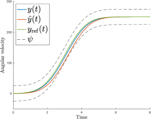
Figure 3: Outputs and reference, with error boundary.

We stress that the estimate in (12) is very conservative. To demonstrate this aspect, we run a second simulation, where we chose $\tau=0.2$, and $T=1$. The results of this simulation are labeled as $\hat{y},\hat{u}$, respectively. With this much larger uniform step length, the tracking objective can be satisfied as well, cf. Figures 3 and 4.

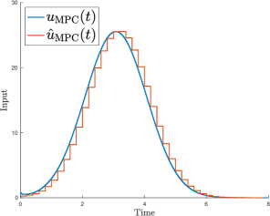
Figure 4: Control inputs.

Note that the maximal applied control value is much smaller than the (conservative) estimate $u_{\rm max}$ which satisfies (11). The simulations have been performed with Matlab using the CasADi framework.

V Conclusion

We proposed a MPC algorithm, which achieves for nonlinear control systems that the output tracks a given reference with predefined accuracy. This control objective was also under consideration in [12] (funnel MPC). While the MPC scheme in [12] uses $L^{\infty}$–functions in the optimal control problem, we showed in this article that the control signal can be restricted to piecewise constant functions with given step length while still guaranteeing the tracking of a reference signal within predefined boundaries. By giving bounds on the sufficient step length for the applied control function, this solves an open problem regarding the applicability of MPC using zero-order hold inputs while maintaining satisfaction of hard output constraints. It is a subject of future research to show that the funnel MPC schemes from [13, 14] for systems with higher relative degree can also be restricted to piecewise constant step functions while still achieving the control objective. Another topic for future research is to investigate whether the sampled-data controller from [20] can be combined with the presented MPC algorithm similar as in [15] to robustly allow for the application of zero-order hold MPC to systems with disturbances and a plant-model mismatch while receiving system data only at sampling times, and restricting the control signal to piecewise constant functions. In the case of a positive outcome, it might be possible to further combine the resulting control scheme with learning techniques like done in [16].

VI Proof of the main result

Throughout this section, let the assumptions of Theorem III.1 hold. In preparation of proving Theorem III.1, we note some observations for later use and recall some results from [20] adapted to the current setting. To achieve that the tracking error $e:=y-y_{\operatorname*{ref}}$ evolves within $\mathcal{F}_{\psi}$ with $\psi\in\mathcal{G}$, it is necessary that the output $y(t)$ of the system (1) is at every time $t\geq t_{0}$ an element of the set

$$\mathcal{D}_{t}:=\left\{\ y\in\mathds{R}^{m}\ \left|\ \vphantom{y\in\mathds{R}^{m}}\left\|y-y_{\operatorname*{ref}}(t)\right\|\leq\psi(t)\ \right.\right\}.$$ (8)

For a $L^{\infty}$–control function $u$ bounded by $u_{\max}>0$ to achieve the control objective on an interval $I\subset\mathds{R}_{\geq 0}$ with $\hat{t}:=\min I$, i.e. ensuring that the tracking error $e$ evolves within $\mathcal{F}_{\psi}$, it is necessary for $u$ to be an element of the set

$$\mathcal{U}_{I}(u_{\max},\hat{y})\!:=\!\left\{\ \!\!\!u\in L^{\infty}(I,\mathds{R}^{m})\!\!\!\ \left|\ \vphantom{\!\!\!u\in L^{\infty}(I,\mathds{R}^{m})\!\!\!}\!\!\!\!\!\begin{array}[]{l}y(t;\hat{t},\hat{y},u)\in\mathcal{D}_{t}\!\!\ \forall\,t\in I,\\ \left\|u\right\|_{\infty}\leq u_{\max}\end{array}\!\!\!\!\!\!\!\ \right.\right\}\!,$$

where $\hat{y}\in\mathcal{C}([t_{0}-\sigma,\hat{t}],\mathds{R}^{m})$ with $\hat{y}(t)\in\mathcal{D}_{t}$ for all $t\in[t_{0},\hat{t}]$. Consequently, for a step function with partition $\mathcal{P}$ to achieve the control objective it has to be an element of

$$\mathcal{U}_{I}^{\mathcal{P}}(u_{\max},\hat{y}):=\mathcal{T}_{\mathcal{P}}(I,\mathds{R}^{m})\cap\mathcal{U}_{I}(u_{\max},\hat{y}).$$

A solution of the system (1) which fulfills the control objective up to a time $\nu>t_{0}$ is an element of the set

$$\mathcal{Y}_{\nu}\!:=\!\left\{\ \!\!\zeta\!\in\!\mathcal{C}([t_{0}-\sigma,\infty),\mathds{R}^{m})\!\!\!\ \left|\ \vphantom{\!\!\zeta\!\in\!\mathcal{C}([t_{0}-\sigma,\infty),\mathds{R}^{m})\!\!\!}\!\!\!\!\begin{array}[]{l}\zeta=y^{0},\!\ \forall\,t\!\in\![t_{0},\nu]\!:\\ \zeta(t)\!-\!y_{\operatorname*{ref}}(t)\!\in\!\mathcal{D}_{t}\end{array}\!\!\!\!\!\ \right.\right\}\!.$$

This is the set of all functions $\zeta\in\mathcal{C}([t_{0}-\sigma,\infty),\mathds{R}^{m})$ which coincide with $y^{0}$ on $[t_{0}-\sigma,t_{0}]$ and evolve within the funnel $\mathcal{D}_{t}$ on the interval $[t_{0},\nu]$. With this notation, we may state the following existence result, which is a particular version of [20, Lemma 1.2].

Lemma VI.1

Under the assumptions of Theorem III.1, there exist constants $f_{\max}$, $g_{\max}$, $g_{\min}>0$ such that for every $\nu>t_{0}$, $\zeta\in\mathcal{Y}_{\nu}$, $z\in\mathds{R}^{n}\backslash\left\{0\right\}$ and $t\in[t_{0},\nu)$

$$f_{\max} \geq\left\|f((\mathbf{T}(\zeta))|_{[t_{0},\nu)})\right\|_{\infty},$$ (9)

$$g_{\max} \geq\left\|g((\mathbf{T}(\zeta))|_{[t_{0},\nu)})\right\|_{\infty},$$

$$g_{\min} \leq\frac{\left\langle z,g((\mathbf{T}(\zeta))|_{[t_{0},\delta)}(t))z\right\rangle}{\left\|z\right\|^{2}}.$$

In virtue of Lemma VI.1 let

$$\kappa_{0} :=\left\|\psi\tfrac{\text{d}}{\text{d}t}1/\psi\right\|_{\infty}+\left\|1/\psi\right\|_{\infty}(f_{\max}+\|\dot{y}_{\operatorname*{ref}}\|_{\infty}),$$

$$\beta >\tfrac{2\kappa_{0}}{g_{\min}\left\|\psi\right\|_{\infty}},$$

$$\kappa_{1} :=\kappa_{0}+\left\|1/\psi\right\|_{\infty}g_{\max}\beta,$$

and $\tau\in(0,\kappa_{0}/\kappa_{1}^{2}]$. It has been proven in [20, Theorem 2.8] that the application of the ZoH control

$$\,u_{\rm ZoH}(t)=\begin{cases}0,\!\!&\|e(t_{i})\|<\psi(t_{i})\left(1-\tfrac{\kappa_{0}^{2}}{\kappa_{1}^{2}}\right),\\ -\beta\tfrac{e(t_{i})}{\|e(t_{i})\|^{2}},\!\!&\|e(t_{i})\|\geq\psi(t_{i})\left(1-\tfrac{\kappa_{0}^{2}}{\kappa_{1}^{2}}\right),\end{cases}$$ (10)

to the system (1), for $t\in[t_{i},t_{i}+\tau)$ with $t_{i}=i\tau$, $i\in\mathds{N}_{0}$, yields $y(t;t_{0},y^{0},u_{\rm ZoH})\in\mathcal{D}_{t}$ for all $t\in[t_{0},\infty)$. Note that $\left\|u_{\rm ZoH}\right\|_{\infty}\leq\tfrac{\beta}{1-\kappa_{0}^{2}/\kappa_{1}^{2}}$. Consequently $\mathcal{U}_{[t_{0},\infty)}^{\mathcal{P}}(u_{\max},y_{0})\neq\emptyset$ for $u_{\max}\geq\tfrac{\beta}{1-\kappa_{0}^{2}/\kappa_{1}^{2}}$ and all partitions $\mathcal{P}$ of $[t_{0},\infty)$ with $\left|P\right|\leq\kappa_{0}/\kappa_{1}^{2}$. If, for $\hat{t}\in\tau\mathds{N}$, a on the interval $[t_{0},\hat{t}]$ piece-wise constant control $u\in\mathcal{U}_{[t_{0},\hat{t}]}^{\mathcal{P}}(u_{\max},y^{0})$ is applied to the system (1) on the interval $[t_{0},\hat{t}]$, then the tracking error $e$ evolves within the funnel $\mathcal{F}_{\psi}$, i.e. $y(t;t_{0},y^{0},u)\in\mathcal{D}_{t}$ for all for all $t\in[t_{0},\hat{t}]$. In particular, $y(\hat{t};t_{0},y^{0},u)\in\mathcal{D}_{\hat{t}}$. Then, $y(\cdot;t_{0},y^{0},u)$ can be extended to a function $\zeta\in\mathcal{C}([t_{0}-\sigma,\infty),\mathds{R}^{m})$, i.e. $\zeta|_{[t_{0},\hat{t}]}\equiv y(\cdot;t_{0},y^{0},u)$. The function $\zeta$ is an element of $\mathcal{Y}_{\hat{t}}$. Therefore, the prerequisites of [20, Theorem 2.8] are fulfilled with the same constants as in (10). This means that the application of $u_{\rm ZoH}$ to the system (1) on the interval $[\hat{t},\infty)$ ensures that the tracking error $e$ evolves within the funnel $\mathcal{F}_{\psi}$ on the interval $[\hat{t},\infty)$. Thus, we have $u_{\rm ZoH}\in\mathcal{U}_{[t_{0},\hat{t}]}^{\mathcal{P}}(u_{\max},y(\hat{t};t_{0},y^{0},u))$.

Summing up our observations, we state the following direct consequence of [20, Lemma 1.2, Theorem 2.8].

Corollary VI.1

Under the assumptions of Theorem III.1, let

$$u_{\max}\geq\tfrac{\beta}{1-\kappa_{0}^{2}/\kappa_{1}^{2}}$$ (11)

and $\mathcal{P}=(t_{k})_{k\in\mathds{N}_{0}}$ be a partition of the interval $[t_{0},\infty)$ with

$$\left|\mathcal{P}\right|\leq\kappa_{0}/\kappa_{1}^{2}.$$ (12)

Then, $\mathcal{U}_{[t_{0},\infty)}^{\mathcal{P}}(u_{\max},y_{0})\neq\emptyset$. Furthermore, for all $k,j\in\mathds{N}_{0},k>j$, we have

$$\ \forall\,u\in\mathcal{U}_{[t_{0},t_{j}]}^{\mathcal{P}}(u_{\max},y^{0})\!:\mathcal{U}_{[t_{0},t_{k}]}^{\mathcal{P}}(u_{\max},y(t_{j};t_{0},y^{0},u))\neq\emptyset.$$ (13)

With these preliminaries at hand, we may now prove Theorem III.1.

Proof of Theorem III.1: According to Corollary VI.1, there exist $u_{\max}>0$ and $\tau>0$ such that $\mathcal{U}_{[t_{0},\infty)}^{\mathcal{P}}(u_{\max},y^{0})\neq\emptyset$ for a partition $\mathcal{P}$ with $\left|\mathcal{P}\right|\leq\tau$. Let $T\geq\delta$ be arbitrary but fixed. $\mathcal{U}_{[t_{0},\infty)}^{\mathcal{P}}(u_{\max},y^{0})\neq\emptyset$ implies that $\mathcal{U}_{[t_{0},t_{0}+T]}^{\mathcal{P}}(u_{\max},y^{0})$ is non-empty as well. Fact (13) implies that if, at every time instance $\hat{t}\in t_{0}+\delta\mathds{N}_{0}$ in Step 3 of Algorithm 1, a control $u\in\mathcal{U}_{[\hat{t},\hat{t}+T]}^{\mathcal{P}}(u_{\max},\hat{y})$ is applied to the system (1), where $\hat{y}=y(\hat{t};t_{0},y^{0},u_{\rm MPC})$ is the output of the system at time $\hat{t}$, then $\left\|e(t)\right\|=\left\|y(t)-y_{\operatorname*{ref}}(t)\right\|\leq\psi(t)$ for all $t\in[\hat{t},\hat{t}+\delta]$ and $\mathcal{U}_{[\hat{t}+\delta,\hat{t}+\delta+T]}^{\mathcal{P}}(u_{\max},y(\hat{t}+\delta;\hat{t},\hat{y},u))\neq\emptyset$. In particular, this inductively implies that (i) and (ii) are fulfilled.

Therefore, it only remains to show that if $\mathcal{U}_{[\hat{t},\hat{t}+T]}^{\mathcal{P}}(u_{\max},\hat{y})$ is non-empty for some $\hat{t}\in t_{0}+\delta\mathds{N}_{0}$ and $\hat{y}\in\mathcal{C}([t_{0}-\sigma,\hat{t}],\mathds{R}^{m})$ with $\hat{y}(t)\in\mathcal{D}_{t}$ for all $t\in[t_{0},\hat{t}]$, then the OCP (5) has a solution $u^{\star}\in\mathcal{U}_{[\hat{t},\hat{t}+T]}^{\mathcal{P}}(u_{\max},\hat{y})$. To prove this, assume $\mathcal{U}_{[\hat{t},\hat{t}+T]}^{\mathcal{P}}(u_{\max},\hat{y})\neq\emptyset$ for $\hat{t}\in t_{0}+\delta\mathds{N}_{0}$ and $\hat{y}\in\mathcal{C}([t_{0}-\sigma,\hat{t}],\mathds{R}^{m})$ with $\hat{y}(t)\in\mathcal{D}_{t}$ for all $t\in[t_{0},\hat{t}]$. Define the function $J:L^{\infty}([\hat{t},\hat{t}+T],\mathds{R}^{m})\to\mathds{R}\cup\left\{\infty\right\}$ by

$$J(u)=\int_{\hat{t}}^{\hat{t}+T}\ell(t,y(t;\hat{t},\hat{y},u),u)\ \text{d}t.$$

Step 1: Adapting [12, Theorem 4.3] to the current setting we show that $J(u)<\infty$ for $u\in L^{\infty}([\hat{t},\hat{t}+T],\mathds{R}^{m})$ with $\left\|u\right\|\leq u_{\max}$ if and only if $u\in\mathcal{U}_{[\hat{t},\hat{t}+T]}(u_{\max},\hat{y})$. Given $u\in\mathcal{U}_{T}(u_{\max},\hat{y})$, it follows from the definition of $\mathcal{U}_{T}(u_{\max},\hat{y})$ that $e(t):=y(t;\hat{t},\hat{y},u)-y_{\operatorname*{ref}}(t)\in\mathcal{D}_{t}$ for all $t\in[\hat{t},\hat{t}+T]$. Thus,

$$\forall\,t\in[\hat{t},\hat{t}+T]:\ \left\|e(t)\right\|\leq\psi(t).$$

Therefore, $\ell(t,y(t;\hat{t},\hat{y},u),u)=\tilde{\ell}(t,y(t;\hat{t},\hat{y},u),u)$ for all $t\in[\hat{t},\hat{t}+T]$. Hence,

$$J(u)=\!\int_{\hat{t}}^{\hat{t}+T}\!\!\!\tilde{\ell}(t,y(t;\hat{t},\hat{y},u),u)\ \text{d}{t}\leq\|{\tilde{\ell}}\|_{{L^{1}{(\mathcal{D}^{\varphi}}\times\mathcal{B}_{u_{\max}})}}\!\!<\!\infty.$$

To show the opposite direction, let $u\in L^{\infty}([\hat{t},\hat{t}+T],\mathds{R}^{m})$ with $J(u)<\infty$. Assume there exists $\tilde{t}\in(\hat{t},\hat{t}+T]$ with $\left\|e(\tilde{t})\right\|>\psi(\tilde{t})$. By continuity of the involved functions, there exists $\varepsilon\in(0,\tilde{t}-\hat{t})$ with $\left\|e(t)\right\|>\psi(t)$ for all $t\in(\tilde{t}-\varepsilon,\tilde{t})$. Thus,

$$J(u) =\int_{\hat{t}}^{\hat{t}+T}\ell(t,y(t;\hat{t},\hat{y},u),u)\ \text{d}t$$

$$\geq\int_{\tilde{t}-\varepsilon}^{\tilde{t}}\ell(t,y(t;\hat{t},\hat{y},u),u)\ \text{d}t=\varepsilon\cdot\infty=\infty.$$

Step 2: We prove that $\min_{u\in\mathcal{U}_{[\hat{t},\hat{t}+T]}^{\mathcal{P}}(u_{\max},\hat{y})}J(u)$ exists. Since $\mathcal{U}_{[\hat{t},\hat{t}+T]}^{\mathcal{P}}(u_{\max},\hat{y})\subset\mathcal{U}_{[\hat{t},\hat{t}+T]}(u_{\max},\hat{y})$, the set $\mathcal{U}_{[\hat{t},\hat{t}+T]}(u_{\max},\hat{y})$ is non-empty by assumption. Since ${J(u)\geq 0}$ for all $u\in\mathcal{U}_{[\hat{t},\hat{t}+T]}^{\mathcal{P}}$, the infimum $J^{\star}:=\inf_{u\in\mathcal{U}_{[\hat{t},\hat{t}+T]}^{\mathcal{P}}(u_{\max},\hat{y})}J(u)$ exists. Let $(u_{k})_{k\in\mathds{N}_{0}}\in\left(\mathcal{U}_{[\hat{t},\hat{t}+T]}^{\mathcal{P}}(u_{\max},\hat{y})\right)^{\mathds{N}_{0}}$ be a minimizing sequence, meaning $J(u_{k})\to J^{\star}$. By choice in the Algorithm 1 we known that $(t_{0}+\delta k)_{k\in\mathds{N}_{0}}$ is a subsequence of the partition $\mathcal{P}=(t_{k})_{k\in\mathds{N}_{0}}$. Therefore, there exists $M,N\in\mathds{N}_{0}$, $N\geq M$ with $t_{M}=\hat{t}$ and $t_{n}>\hat{t}+T$ for all $n>N$. Define $u_{i,k}:=u_{k}(t_{i})$ for $i=M,\ldots,N$. For every $i=M,\ldots,N$, $(u_{i,k})_{k\in\mathds{N}_{0}}$ is a sequence in $\mathds{R}^{m}$ with $\left\|u_{i,k}\right\|\leq u_{\max}$ for all $k\in\mathds{N}$. Thus, it has a limit point $u_{i}^{\star}\in\mathds{R}^{m}$. The function $u^{\star}$ defined by $u^{\star}|_{[t_{i},t_{i+1})\cap[\hat{t},\hat{t}+T]}:=u^{\star}_{i}$ is an element of $\mathcal{T}_{\mathcal{P}}([\hat{t},\hat{t}+T],\mathds{R}^{m})$ with $\left\|u^{\star}\right\|\leq u_{\max}$. Up to subsequence, $u_{k}$ converges uniformly to $u^{\star}$. Let $y_{k}:=y(\cdot;t_{0},y^{0},u_{k})$ be the sequence of associated responses. By an adaption of the Steps 2, 3 of the proof of [12, Theorem 4.6] to the current setting, we may infer that $(y_{k})$ has a subsequence (which we do not relabel) that converges uniformly to $y^{\star}(\cdot;\hat{t},\hat{y},u^{\star})$. It remains to show $u^{\star}\in\mathcal{U}_{[\hat{t},\hat{t}+T]}^{\mathcal{P}}(u_{\max},\hat{y})$. This means to show $y^{\star}(t)\in\mathcal{D}_{t}$ for all $t\in[\hat{t},\hat{t}+T]$. Assume there exists $\tau\in(\hat{t},\hat{t}+T]$ with $y^{\star}(\tau)\notin\mathcal{D}_{\tau}$, i.e. $\left\|y^{\star}(\tau)-y_{\operatorname*{ref}}(\tau)\right\|>\psi(\tau)$. There exists $\varepsilon>0$ with $\left\|y^{\star}(\tau)-y_{\operatorname*{ref}}(\tau)\right\|>\psi(\tau)+\varepsilon$. Since the uniform convergence of $(y_{k})$ towards $y^{\star}$ implies pointwise convergence of $(y_{k})$, there exists $K>0$ such that $\left\|y^{\star}(\tau)-y_{k}(\tau)\right\|<\varepsilon$ for all $k\geq K$. Furthermore, $\left\|y_{k}(\tau)-y_{\operatorname*{ref}}(\tau)\right\|\leq\psi(\tau)$ since $u_{k}\in\mathcal{U}_{[\hat{t},\hat{t}+T]}^{\mathcal{P}}(u_{\max},\hat{y})$ for all $k\in\mathds{N}_{0}$. This raises the following contradiction for $k\geq K$.

$$\psi(\tau)+\varepsilon <\left\|y^{\star}(\tau)-y_{\operatorname*{ref}}(\tau)\right\|$$

$$\leq\left\|y^{\star}(\tau)-y_{k}(\tau)\right\|+\left\|y_{k}(\tau)-y_{\operatorname*{ref}}(\tau)\right\|$$

$$\leq\varepsilon+\psi(\tau).$$

Thus, $u^{\star}\in\mathcal{U}_{[\hat{t},\hat{t}+T]}^{\mathcal{P}}(u_{\max},\hat{y})$. It remains to show that $J^{\star}=J(u^{\star})$ and $J(u^{\star})=\min_{u\in\mathcal{U}_{[\hat{t},\hat{t}+T]}^{\mathcal{P}}(u_{\max},\hat{y})}J(u)$, which follows along the lines of Steps 6, 7 of the proof of [12, Theorem 4.6]. $\Box$

References

• [1] L. Grüne and J. Pannek, Nonlinear Model Predictive Control: Theory and Algorithms.   London: Springer, 2017.
• [2] J. B. Rawlings, D. Q. Mayne, and M. Diehl, Model predictive control: theory, computation, and design.   Nob Hill Publishing Madison, WI, 2017, vol. 2.
• [3] H. Chen and F. Allgöwer, “A quasi-infinite horizon nonlinear model predictive control scheme with guaranteed stability,” Automatica, vol. 34, no. 10, pp. 1205–1217, 1998.
• [4] D. Q. Mayne, J. B. Rawlings, C. V. Rao, and P. O. Scokaert, “Constrained model predictive control: Stability and optimality,” Automatica, vol. 36, no. 6, pp. 789–814, 2000.
• [5] J.-M. Coron, L. Grüne, and K. Worthmann, “Model predictive control, cost controllability, and homogeneity,” SIAM Journal on Control and Optimization, vol. 58, no. 5, pp. 2979–2996, 2020.
• [6] A. Boccia, L. Grüne, and K. Worthmann, “Stability and feasibility of state constrained MPC without stabilizing terminal constraints,” Systems & control letters, vol. 72, pp. 14–21, 2014.
• [7] W. Esterhuizen, K. Worthmann, and S. Streif, “Recursive feasibility of continuous-time model predictive control without stabilising constraints,” IEEE Control Systems Letters, vol. 5, no. 1, pp. 265–270, 2020.
• [8] W.-H. Chen, J. O’Reilly, and D. J. Ballance, “On the terminal region of model predictive control for non-linear systems with input/state constraints,” International journal of adaptive control and signal processing, vol. 17, no. 3, pp. 195–207, 2003.
• [9] A. H. González and D. Odloak, “Enlarging the domain of attraction of stable MPC controllers, maintaining the output performance,” Automatica, vol. 45, no. 4, pp. 1080–1085, 2009.
• [10] T. Manrique, M. Fiacchini, T. Chambrion, and G. Millérioux, “MPC tracking under time-varying polytopic constraints for real-time applications,” in 2014 European Control Conference (ECC).   IEEE, 2014, pp. 1480–1485.
• [11] T. Berger, C. Kästner, and K. Worthmann, “Learning-based Funnel-MPC for output-constrained nonlinear systems,” IFAC-PapersOnLine, vol. 53, no. 2, pp. 5177–5182, 2020.
• [12] T. Berger, D. Dennstädt, A. Ilchmann, and K. Worthmann, “Funnel Model Predictive Control for Nonlinear Systems with Relative Degree One,” SIAM Journal on Control and Optimization, vol. 60, no. 6, pp. 3358–3383, 2022.
• [13] T. Berger and D. Dennstädt, “Funnel MPC with feasibility constraints for nonlinear systems with arbitrary relative degree,” IEEE Control Systems Letters, 2022.
• [14] ——, “Funnel MPC for nonlinear systems with arbitrary relative degree,” arXiv preprint arXiv:2308.12217, 2023.
• [15] T. Berger, D. Dennstädt, L. Lanza, and K. Worthmann, “Robust Funnel Model Predictive Control for output tracking with prescribed performance,” arXiv preprint arXiv:2302.01754, 2023.
• [16] L. Lanza, D. Dennstädt, T. Berger, and K. Worthmann, “Safe continual learning in MPC with prescribed bounds on the tracking error,” arXiv preprint arXiv:2304.10910v2, 2023.
• [17] A. Ilchmann, E. P. Ryan, and C. J. Sangwin, “Tracking with prescribed transient behaviour,” ESAIM: Control, Optimisation and Calculus of Variations, vol. 7, pp. 471–493, 2002.
• [18] T. Berger, A. Ilchmann, and E. P. Ryan, “Funnel control of nonlinear systems,” Math. Control Signals Syst., vol. 33, pp. 151–194, 2021.
• [19] ——, “Funnel control–a survey,” arXiv preprint arXiv:2310.03449, 2023.
• [20] L. Lanza, D. Dennstädt, K. Worthmann, P. Schmitz, G. D. Şen, S. Trenn, and M. Schaller, “Control and safe continual learning of output-constrained nonlinear systems,” arXiv preprint arXiv:2303.00523, 2023.
• [21] T. Berger, M. Puche, and F. L. Schwenninger, “Funnel control in the presence of infinite-dimensional internal dynamics,” Syst. Control Lett., vol. 139, p. Article 104678, 2020.
• [22] ——, “Funnel control for a moving water tank,” Automatica, vol. 135, p. Article 109999, 2022.
• [23] C. I. Byrnes and A. Isidori, “Asymptotic stabilization of minimum phase nonlinear systems,” IEEE Trans. Autom. Control, vol. 36, no. 10, pp. 1122–1137, 1991.
• [24] T. Berger, H. H. Lê, and T. Reis, “Funnel control for nonlinear systems with known strict relative degree,” Automatica, vol. 87, pp. 345–357, 2018.
• [25] H. T. Pham, “Control methods of powertrains with backlash and time delay,” Ph.D. dissertation, Hamburg University of Technology, Hamburg, 2019.
• [26] S. Drücker, “Servo-constraints for inversion of underactuated multibody systems,” PhD Thesis, Hamburg University of Technology, 2022. [Online]. Available: http://hdl.handle.net/11420/11463
• [27] A. Ilchmann, “Non-identifier-based adaptive control of dynamical systems: A survey,” IMA Journal of Mathematical Control and Information, vol. 8, no. 4, pp. 321–366, 1991.