Wiener Chaos in Kernel Regression:
Towards Untangling Aleatoric and Epistemic Uncertainty
Institute of Energy Systems Energy Efficiency and Energy Economics (ie3)
TU Dortmund University
44227 Dortmund, Germany
timm.faulwasser@ieee.org
&Oleksii Molodchyk
Institute of Energy Systems Energy Efficiency and Energy Economics (ie3)
TU Dortmund University
44227 Dortmund, Germany
oleksii.molodchyk@tu-dortmund.de
Abstract
Gaussian Processes (GPs) are a versatile method that enables different approaches towards learning for dynamics and control. Gaussianity assumptions appear in two dimensions in GPs: The positive semi-definite kernel of the underlying reproducing kernel Hilbert space is used to construct the co-variance of a Gaussian distribution over functions, while measurement noise (i.e. data corruption) is usually modeled as i.i.d. additive Gaussian. In this note, we relax the latter Gaussianity assumption, i.e., we consider kernel ridge regression with additive i.i.d. non-Gaussian measurement noise. To apply the usual kernel trick, we rely on the representation of the uncertainty via polynomial chaos expansions, which are series expansions for random variables of finite variance introduced by Norbert Wiener. We derive and discuss the analytic solution to the arising Wiener kernel regression. Considering a polynomial system as numerical example, we show that our approach allows to untangle the effects of epistemic and aleatoric uncertainties.
Keywords non-Gaussian distribution kernel regression polynomial chaos expansion aleatoric and epistemic uncertainty
1 Introduction
Gaussian Processes (GPs) are an established non-parametric supervised learning method which can be used for classification and regression. The core idea evolves around Gaussian distributions over functions with continuous domain. In the context of learning for dynamics and control early successful application of GPs, e.g., to model dynamic systems can be traced back at least to Murray-Smith et al. (1999). Early application for predictive control is considered by Kocijan et al. (2003), while Deisenroth (2010) discusses the use of GPs in reinforcement learning; see also Rasmussen and Williams (2006) for an introductory reference on GPs. Due to space constraints, we do not provide a detailed overview of existing results but rather refer to the recent papers (Deisenroth et al., 2013; Berkenkamp and Schoellig, 2015; Hewing et al., 2019) and references therein for further details.
A particular appealing feature of GPs is the posterior co-variance estimate of the predictions. This estimate is, e.g., of interest in Bayesian optimization (Heo and Zavala, 2012) as it allows to approach the exploration-exploitation trade-off. Moreover, the posterior co-variance estimate is of interest whenever GPs are trained to predict exogenous disturbances, e.g., energy consumption and renewable power generation (Heo and Zavala, 2012; Van der Meer et al., 2018; Drgoňa et al., 2020; Chen et al., 2013).
On a formal level the co-variance estimate of GPs is closely related to the underlying kernel and to the Gaussianity assumption made on the measurement noise (Kanagawa et al., 2018). Indeed there exists a close relation between Reproducing Kernel Hilbert Spaces (RKHS) and GPs, see, e.g., the recent treatments (Kanagawa et al., 2018; Rasmussen and Williams, 2006) and the classic reference (Kailath, 1971).
In the present paper, we take a fresh look at kernel regression problems with noise corrupted data samples, whereby the measurement noise does not need to be Gaussian. Specifically, we combine Polynomial Chaos Expansions (PCE), which originated in the most-cited journal paper of Wiener (1938), with kernel regression problems. Recently, PCE has seen use in data-driven control of linear systems (Pan et al., 2023; Faulwasser et al., 2023). While the link between PCE and the RKHS underlying GPs settings has, e.g., been investigated by Yan et al. (2018), a numerical comparison of both approaches as function approximators is conducted by Gratiet et al. (2016). However, the previous two papers as well as the work of Torre et al. (2019) do not explore the potential of considering PCE-based measurement noise models in regression problems for dynamics and control.
The contributions and the outline of the present paper are as follows: After a concise problem statement in Section 2, we consider an intrusive uncertainty quantification approach for kernel regression problems in Section 3. Put differently, we use the PCE framework to quantify the effect of non-Gaussian measurement noise on the prediction obtained via kernel ridge regression. Moreover, we discuss the relation of this aleatoric uncertainty to the classic posterior co-variance estimate which measures epistemic uncertainty. We also draw upon a numerical example to illustrate how our approach allows to untangle aleatoric and epistemic uncertainty in Section 4. The paper ends with conclusions and outlook in Section 5.
2 Problem Statement and Preliminaries
The weight-space view of GPs with features
Following the classic exposition of Rasmussen and Williams (2006) we recall the weight-space view on GPs. Consider the data obtained from sampling the unknown function . For the sake of simplified exposition and to limit the notion overhead, we henceforth consider the setting that . Moreover, we use the shorthands and . The data is obtained via
| (1) |
i.e., from measurements of the output of corrupted by individually independently distributed (i.i.d.) white Gaussian noise of known distribution . Suppose that the unknown function is of the form with the feature map . The learned GP based on the data , on the distribution of the measurement noise , and on the prior distribution of the weights is given by
| (2a) | ||||
| (2b) | ||||
where is the evaluation of the kernel function for ; is the column vector obtained by evaluating the kernel on the entire data , and is the square Gram matrix with evaluated for all samples . Put differently, the learned GP predicts for each argument a Gaussian random variable as given by (2).
The close relation of the mean predictor (2a) to kernel ridge regression and to the representer theorem (Kimeldorf and Wahba, 1970; Schölkopf et al., 2001) is well-known (Rasmussen and Williams, 2006; Kanagawa et al., 2018). Indeed, the underlying key assumption is that the unknown function is an element of the RKHS spanned by the kernel , which in case of the feature function reads .
Problem statement
We consider the non-Gaussian extension to (1) which reads
| (3) |
i.e., the additive noise is modeled as an i.i.d. random variable of known—not necessarily Gaussian—distribution characterized by the probability measure . Specifically, the probability space comprises the set of outcomes , the sigma-algebra , and the probability measure . Hence does not need to be Gaussian. Its nature implies that any element of has finite expectation and variance. The scalar realizations of are written as and they take values in . Therefore, in (1) and (3) refers to the random and hence unknown noise samples corrupting the measurements.
Henceforth, given the data set obtained from (3) and supposing knowledge of the distribution of the additive measurement noise , we are interested in deriving an extension to the classic GP predictor (2) which allows for non-Gaussian noise on the measurements. To this end, we exploit the structure of the considered probability space.
Fundamentals of polynomial chaos expansions
PCE is an established method for uncertainty quantification and it dates back to Wiener (1938). It is based on the fact that any Hilbert space can be spanned by a polynomial basis, see Sullivan (2015) for a general introduction. PCE is frequently considered in system and control (Kim et al., 2013; Mesbah et al., 2014; Paulson et al., 2014) and we refer to Faulwasser et al. (2023); Pan et al. (2023) for applications in data-driven control. Consider an orthogonal polynomial basis which spans the probability space , i.e.,
where is the Kronecker delta and is the induced norm of . Any real-valued scalar random variable can be expressed in the basis via the series expansion
where is called the -th PCE coefficient. It is customary when working with PCE to consider the first basis function to be and that all other basis functions have zero mean. Indeed, depending on the considered distribution of , one adapts the algebraic structure of the basis and its argument (Xiu and Karniadakis, 2002; Kim et al., 2013).
From a computational point of view, infinite PCE series are impractical and hence only a finite number of terms are usually considered. This, however, may induce truncation errors (Mühlpfordt et al., 2018). It is well-known that random variables following some widely-used distributions admit exact finite-dimensional PCEs with only two terms in suitable polynomial bases, see Xiu and Karniadakis (2002). This observation gives rise to the following definition of exact PCE representations.
Definition 1 (Exact PCE representation (Mühlpfordt et al., 2018)).
The PCE of a random variable is said to be exact with dimension if .
Given a PCE of finite dimension , the expected value, the variance, and the co-variance of entries in a vector-valued random variable with can be efficiently calculated from the PCE coefficients
| (4) |
where and is the Hadamard product (Sullivan, 2015).
3 Main Results
Next, we consider the PCE approach to tackle the regression problem derived from the non-Gaussian setting (3). To this end, we suppose that the i.i.d. additive measurement noise entails an exact PCE of dimension , i.e., . Note that for all samples the PCE coefficients are the same due to the i.i.d.-ness of the random variables .
Regression with noise description
Similar to usual kernel regression problems, we consider the linear ansatz via feature map , i.e., we presume the structure . The additive noise leads to the following regularized regression problem
Note that for each data sample the -loss includes the unknown noise realizations . One possible workaround is to neglect the realizations of the measurement noise and work with the corrupted measurements . Alternatively, we consider the random variable description of . Rewriting the above objective in the expected value sense of statistical learning yields the following regression problem
| (5) |
Recall that the data consists of real-valued tuples while in the learning problem the measurement noise is considered as i.i.d. random variables. Hence the weights are also lifted to this space. It is easy to see that if one does lift the decision variables to then in the first-order stationarity condition, the realization of matches the measurement uncertainty to reduce the expected loss. We refer to Bienstock et al. (2014) for a corresponding discussion of stochastic optimization problems arising in energy systems.
Wiener kernel regression
To avoid the technicalities of solving the regression in the infinite-dimensional space directly, we use the PCE representation of the noise and of the weights . In particular, the weights are component-wise presented in the joint scalar basis with
The basis is of dimension , it includes the bases for all . Put differently, we consider one basis polynomial for the mean and basis polynomials for the non-mean parts of corresponding to each data sample . We note that the i.i.d. property of is reflected in the fact that the bases for and differ in their arguments and . This way, two random variables of the same distribution—and hence living in the same space—can be distinguished in their PCE representations, while their PCE coefficients are equal. Using the joint basis we arrive at the PCE-reformulated problem
| (6) |
where is the PCE representation of with vectorized PCE coefficients and scalar basis functions . We refer to the reformulated problem (6) as Wiener kernel regression. Its solution is given in the following lemma.
Lemma 1 (Correspondence of optimization problems).
Suppose that for all data samples the i.i.d. additive measurement noise admits an exact PCE of dimension , i.e., . Then the following statements hold:
- i)
- ii)
Proof.
Due to space limitations we only sketch the main steps of the proof. The assumption of an exact PCE of dimension for all gives that , i.e., the PCE for reads and has a dimension corresponding to the number of available data samples plus one extra dimension for the mean . The first part of the objective in (6) can be rewritten as
Similarly to the objective reformulations considered for stochastic data-driven optimal control by Faulwasser et al. (2023), we exploit that the measurement noise is i.i.d. and that all PCE basis functions with have zero mean. Next we set and according to (7b). Utilizing that for any and with the help of (4), we rewrite the objective in (6) as
where we also exploit that (6) is an unconstrained minimization of a strictly convex quadratic function over a real-valued vector space of finite dimension and hence there exists a unique minimizer. Observe that without loss of generality we swapped the summations in the equation above. Hence the above problem can be solved for each PCE dimension individually. Indeed for each PCE dimension it corresponds to a usual kernel regression with regularized loss. Hence we obtain (7a) and the computation of follows from the PCE dimension and the i.i.d.-ness of the random variables . This proves Assertion ii).
Assertion i) is shown via contradiction similar to (Pan et al., 2023, Prop. 1): Recall the assumption of exact PCEs for and the corresponding joint PCE basis. Now consider an extension of the joint basis for and suppose that the optimal solution admits non-zero coefficients beyond the first basis functions. However, these non-zero coefficients strictly increase the considered -objective as the corresponding coefficients for are zero. ∎
Under the assumptions of the above lemma we can now give the Wiener kernel regression for the non-Gaussian setting of (3). The -optimal prediction is given by the scalar random variable as
| (8) |
Observe that is given as a linear combination of finitely many scalar basis functions of the underlying probability space . Moreover, the term is identical for all PCE dimensions. The above result can be generalized (at the expense of a slightly more technical proof) to the case and to other convex loss functions.
Quantification of aleatoric and epistemic uncertainty
The distinction of epistemic and aleatoric uncertainties is an established concept in ML (Hüllermeier and Waegeman, 2021; Umlauft et al., 2020). While the former refers to uncertainty due to a lack of model knowledge or due to a lack of data, the latter refers to the uncertainty which is inherently due to randomness (e.g. measurement noise). Hence it remains to discuss the differences and commonalities of the classic GP prediction (2) and (8). The relation between moments and PCE coefficients leads to the following result.
Lemma 2.
Suppose that for all data samples the i.i.d. additive measurement noise has an exact PCE of dimension . Then, we have
-
i)
(9a) -
ii)
Specifically, for the choice implies that the GP mean value prediction from (2a) is equivalent to .
-
iii)
Moreover, for all it holds that
(9b)
Proof.
We sketch only the main steps. i) Follows directly from (4). First notice that in the Hermite polynomial series a zero-mean Gaussian can be represented via PCE with while the coefficients of are and , which shows ii). iii) the variance of is . Hence implies (9a), where we used that and for Hermite polynomials. Applying (4) yields
The careful reader has surely recognized the difference of the classic GP variance from (2b) and the variance of the optimal PCE solution to the Wiener kernel regression (9b). Notice that both expressions do not depend on the actually acquired measurements but only on the data samples . However, observe that the constant in (9b) depends on the norm of the basis functions used to model the i.i.d. measurement noise, i.e., it depends on the distribution of the noise.
It is well-known that the classic GP variance corresponds to the Gaussian distribution of the next prediction conditioned on the data, i.e. on the samples and measurements via the co-variance encoded in the underlying kernel. Neglecting the measurement noise for a minute, one can say that is the variance in the prediction due to the finite number of considered data samples, i.e., for from (2b) captures the epistemic uncertainty of the mean value predictor (2a). For a formal analysis that in the infinite data limit and for Lipschitz continuous kernels holds, see, e.g., Lederer et al. (2019); Kanagawa et al. (2018). In the case of white additive measurement noise, even if a kernel allows to reconstruct a function exactly from data, the additive structure of (2b) implies that the posterior GP variance is fundamentally bounded from below by the variance of the measurement noise .
In contrast, from (9b) can be understood as the result of propagating the not necessarily Gaussian measurement noise through the linear mean value predictor. Hence, quantifies the effect of the aleatoric uncertainty on the prediction. A formal convergence analysis of in view of the the available data is open at this point. Our numerical experiments, however, indicate that as the number of data samples increases, the variance goes asymptotically to . Put differently, we observe that as the convergence independent of the distribution of provided that , which directly follows from .
4 Numerical Example – Illustration of Aleatoric and Epistemic Uncertainty
We consider the following scalar discrete-time system from Beckers and Hirche (2016)
| (10) |
where denotes the state at time and the additive noise is i.i.d. First we assume that follow the standard normal distribution , i.e., and in the Hermite basis. We extend to a non-Gaussian case later. Given exact measurements of , we are interested in predicting the next system state while the right hand side function in (10) is not known. Following Beckers and Hirche (2016), we use a squared-exponential kernel with and .
Gaussian measurement noise
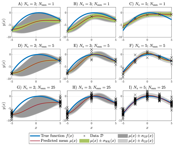
We train the above-mentioned GP using data obtained at different linearly-spaced locations within . The results are depicted in Figure 1, where data points are marked by black crosses. The first row of plots A)-C) shows results in which the data was obtained at different locations. This experiment is repeated increasing number of samples per location in plots A)-C), D)-F), and G)-I), respectively.
In each of the plots, the blue solid line indicates the true function from (10) without measurement noise . The green-shaded tubes are calculated via where corresponds to the predicted mean (red solid line) (2a)/(9a), and is the standard deviation derived from the variance (9b) of the Wiener kernel regression. The GP counterpart of this uncertainty is shown using the dark-gray tube where from (2b). Finally, the light-gray tube illustrates which is the same GP uncertainty with additive measurement noise variance, i.e., for each with , cf. Section 3.
We note that both of the considered GP variance tubes are larger than the green tube obtained via the Wiener kernel regression. As mentioned previously, the GP additionally quantifies the epistemic uncertainty which becomes especially visible when only few locations are considered for training. Indeed, because the chosen squared-exponential kernel has a lengthscale of , the associated RKHS cannot be fully explored within when the samples are taken at only two rather distant locations. Plots A), D), and G) of Figure 1 show that as the number of samples () increases, the noise associated uncertainty—i.e., the green tube—shrinks, while the dark-gray tube that includes the epistemic uncertainty remains.
When five linearly-spaced locations are considered the spacing between the neighboring locations in reduces to , which can be covered by the lengthscale of . This results in a much better exploration of the RKHS. As shown in plot C), the dark-gray area coincides with the noise-related green-colored uncertainty tube. As we eliminate this noise-related uncertainty by increasing the number of samples per location, we notice that our kernel regression result improves dramatically, cf. plots F) and I) in Figure 1. However, the posterior variance prediction of the GP (2b) remains quite large due to its additive structure.
Non-Gaussian noise
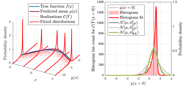
We extend (10) to a non-Gaussian setting, i.e., we consider the i.i.d. , to follow a (skewed) -distribution in which denotes the Gamma function. We set the parameters to and . Thus, the mean of this distribution is , while the variance reads . To comply with Lemma 1, for each , with we choose the basis of dimension with and . The corresponding PCE coefficients are and .
Next we use the same kernel as before to compute via Wiener kernel regression (8). The linearly spaced training data is chosen within with and . We observe that the distribution of is modeled via a linear combination of i.i.d. -distributed random variables. In general, it is difficult to characterize the underlying probability density function analytically. To obtain a numerical approximation, we sample the individual stochastic germs of (8). This way we generate a collection of function realizations for some (finite) subset of outcomes . The left plot of Figure 2 depicts these functions as purple colored solid lines with the true function as well as the predicted mean of the kernel regression. Using , one can create a histogram and a corresponding probability density function (PDF) fit at the selected locations. In the left plot of Figure 2, these fitted PDFs are shown as red solid lines at the locations of the data using samples. On the right hand side of Figure 2, we project onto the plane corresponding to . Here, we plot the histogram of and its fitted PDF as red solid line. For the sake of comparison, we also plot the Gaussians and , which would define the uncertainty tubes stemming from the GP and the Wiener kernel regression, respectively. Similarly to the plots in Figure 1, we also present the distribution of the GP in which . As seen from the right hand side of Figure 2, the fitted distribution of is skewed/asymmetric. That is, the effect of the asymmetrically distributed measurement noise can be quantified via (9b). At this point one has to remark that the epistemic uncertainty is not accurately captured by (9b). However, to this end, one can always rely on the GP posterior variance estimate.
5 Conclusions and Outlook
In the present paper, we have expanded the kernel ridge regression to deal with training data corrupted by i.i.d. additive non-Gaussian noise of finite variance. Relying on the framework of Polynomial Chaos Expansions (PCE) we introduced Wiener kernel regression which handles the non-Gaussian measurement noise effectively. While from an RKHS perspective, the obtained predictive model can in essence still be interpreted as a GP disturbed by measurement noise. In particular, the mean prediction of standard GPs and the proposed Wiener kernel regression coincide. The variance predictions differ, however, in their meaning. While the posterior GP variance is a measure of epistemic uncertainty due to insufficient sampling, the Wiener kernel variance is a measure of the effect of aleatoric measurement uncertainty on the prediction. We have shown via numerical examples how the comparison of both variance estimates allows to untangle epistemic and aleatoric uncertainties.
Our preliminary results point towards further research. As for the presented Wiener kernel regression, there is a need for investigations regarding the properties of the derived variance (9b) with respect to the infinite data limit. Tailored methods for hyperparameter tuning under non-Gaussian noise as well as the consideration of noise corruption on the sample locations are another question for future research. Finally, the proposed approach might provide new avenues to handling the exploration-exploitation trade-off in Bayesian optimization under non-Gaussian noise.
Acknowledgment
The authors thank Ruchuan Ou for helpful feedback on the numerical implementation.
References
- Murray-Smith et al. [1999] R. Murray-Smith, T. Johansen, and R. Shorten. On transient dynamics, off-equilibrium behaviour and identification in blended multiple model structures. In 1999 European Control Conference (ECC), pages 3569–3574. IEEE, 1999.
- Kocijan et al. [2003] J. Kocijan, R. Murray-Smith, C. Rasmussen, and B. Likar. Predictive control with gaussian process models. In The IEEE Region 8 EUROCON 2003. Computer as a Tool., volume 1, pages 352–356. IEEE, 2003.
- Deisenroth [2010] M.P. Deisenroth. Efficient reinforcement learning using Gaussian processes, volume 9. KIT Scientific Publishing, 2010.
- Rasmussen and Williams [2006] C.E. Rasmussen and C.K.I. Williams. Gaussian Processes for Machine Learning. Adaptive computation and machine learning. The MIT Press, 2006.
- Deisenroth et al. [2013] M.P. Deisenroth, D. Fox, and C. Rasmussen. Gaussian processes for data-efficient learning in robotics and control. IEEE Transactions on Pattern Analysis and Machine Intelligence, 37(2):408–423, 2013.
- Berkenkamp and Schoellig [2015] F. Berkenkamp and A. Schoellig. Safe and robust learning control with Gaussian processes. In 2015 European Control Conference (ECC), pages 2496–2501. IEEE, 2015.
- Hewing et al. [2019] L. Hewing, J. Kabzan, and M. Zeilinger. Cautious model predictive control using gaussian process regression. IEEE Transactions on Control Systems Technology, 28(6):2736–2743, 2019.
- Heo and Zavala [2012] Y. Heo and V. Zavala. Gaussian process modeling for measurement and verification of building energy savings. Energy and Buildings, 53:7–18, 2012.
- Van der Meer et al. [2018] D. Van der Meer, M. Shepero, A. Svensson, J. Widén, and J. Munkhammar. Probabilistic forecasting of electricity consumption, photovoltaic power generation and net demand of an individual building using Gaussian processes. Applied Energy, 213:195–207, 2018.
- Drgoňa et al. [2020] J. Drgoňa, J. Arroyo, I. Figueroa, D. Blum, K. Arendt, D. Kim, E. Ollé, J. Oravec, M. Wetter, D. Vrabie, et al. All you need to know about model predictive control for buildings. Annual Reviews in Control, 50:190–232, 2020.
- Chen et al. [2013] N. Chen, Z. Qian, I. Nabney, and X. Meng. Wind power forecasts using Gaussian processes and numerical weather prediction. IEEE Transactions on Power Systems, 29(2):656–665, 2013.
- Kanagawa et al. [2018] M. Kanagawa, P. Hennig, D. Sejdinovic, and B. Sriperumbudur. Gaussian processes and kernel methods: A review on connections and equivalences. arXiv preprint arXiv:1807.02582, 2018.
- Kailath [1971] T. Kailath. RKHS approach to detection and estimation problems–I: Deterministic signals in Gaussian noise. IEEE Transactions on Information Theory, 17(5):530–549, 1971.
- Wiener [1938] N. Wiener. The homogeneous chaos. American Journal of Mathematics, pages 897–936, 1938.
- Pan et al. [2023] G. Pan, R. Ou, and T. Faulwasser. On a stochastic fundamental lemma and its use for data-driven optimal control. IEEE Trans. Automat. Contr., 68:5922 – 5937, 2023.
- Faulwasser et al. [2023] T. Faulwasser, R. Ou, G. Pan, P. Schmitz, and K. Worthmann. Behavioral theory for stochastic systems? A data-driven journey from Willems to Wiener and back again. Annual Reviews in Control, 55:92–117, 2023.
- Yan et al. [2018] L. Yan, X. Duan, B. Liu, and J. Xu. Gaussian processes and polynomial chaos expansion for regression problem: linkage via the RKHS and comparison via the KL divergence. Entropy, 20(3):191, 2018.
- Gratiet et al. [2016] L. Gratiet, S. Marelli, and B. Sudret. Metamodel-based sensitivity analysis: polynomial chaos expansions and Gaussian processes. arXiv preprint arXiv:1606.04273, 2016.
- Torre et al. [2019] E. Torre, S. Marelli, P. Embrechts, and B. Sudret. Data-driven polynomial chaos expansion for machine learning regression. Journal of Computational Physics, 388:601–623, 2019.
- Kimeldorf and Wahba [1970] G.S. Kimeldorf and G. Wahba. A correspondence between Bayesian estimation on stochastic processes and smoothing by splines. The Annals of Mathematical Statistics, 41(2):495–502, 1970.
- Schölkopf et al. [2001] B. Schölkopf, R. Herbrich, and A. Smola. A generalized representer theorem. In International conference on computational learning theory, pages 416–426. Springer, 2001.
- Sullivan [2015] T.J. Sullivan. Introduction to Uncertainty Quantification, volume 63. Springer, 2015.
- Kim et al. [2013] K. K. K. Kim, D. E. Shen, Z. K. Nagy, and R. D. Braatz. Wiener’s polynomial chaos for the analysis and control of nonlinear dynamical systems with probabilistic uncertainties. IEEE Control Systems, 33(5):58–67, 2013.
- Mesbah et al. [2014] A. Mesbah, S. Streif, R. Findeisen, and R.D. Braatz. Stochastic nonlinear model predictive control with probabilistic constraints. In 2014 American Control Conference, pages 2413–2419. IEEE, 2014.
- Paulson et al. [2014] J.A. Paulson, A. Mesbah, S. Streif, R. Findeisen, and R.D. Braatz. Fast stochastic model predictive control of high-dimensional systems. In 53rd IEEE Conference on Decision and Control, pages 2802–2809. IEEE, 2014.
- Xiu and Karniadakis [2002] D. Xiu and G.E. M. Karniadakis. The Wiener-Askey polynomial chaos for stochastic differential equations. SIAM Journal on Scientific Computing, 24(2):619–644, 2002.
- Mühlpfordt et al. [2018] T. Mühlpfordt, R. Findeisen, V. Hagenmeyer, and T. Faulwasser. Comments on quantifying truncation errors for polynomial chaos expansions. IEEE Control Systems Letters, 2(1):169–174, January 2018.
- Bienstock et al. [2014] D. Bienstock, M. Chertkov, and S. Harnett. Chance-constrained optimal power flow: Risk-aware network control under uncertainty. SIAM Review, 56(3):461–495, 2014.
- Hüllermeier and Waegeman [2021] E. Hüllermeier and W. Waegeman. Aleatoric and epistemic uncertainty in machine learning: An introduction to concepts and methods. Machine Learning, 110(3):457–506, 2021.
- Umlauft et al. [2020] J. Umlauft, A. Lederer, T. Beckers, and S. Hirche. Real-time uncertainty decomposition for online learning control, 2020. preprint arXiv:2010.02613.
- Lederer et al. [2019] A. Lederer, J. Umlauft, and S. Hirche. Posterior variance analysis of gaussian processes with application to average learning curves. arXiv preprint arXiv:1906.01404, 2019.
- Beckers and Hirche [2016] T. Beckers and S. Hirche. Equilibrium distributions and stability analysis of Gaussian Process State Space Models. In 2016 IEEE 55th Conference on Decision and Control (CDC). IEEE, 2016.