Boosting Latent Diffusion with Flow Matching

Abstract

Recently, there has been tremendous progress in visual synthesis and the underlying generative models. Here, diffusion models (DMs) stand out particularly, but lately, flow matching (FM) has also garnered considerable interest. While DMs excel in providing diverse images, they suffer from long training and slow generation. With latent diffusion, these issues are only partially alleviated. Conversely, FM offers faster training and inference but exhibits less diversity in synthesis.

We demonstrate that introducing FM between the Diffusion model and the convolutional decoder offers high-resolution image synthesis with reduced computational cost and model size. Diffusion can then efficiently provide the necessary generation diversity. FM compensates for the lower resolution, mapping the small latent space to a high-dimensional one. Subsequently, the convolutional decoder of the LDM maps these latents to high-resolution images. By combining the diversity of DMs, the efficiency of FMs, and the effectiveness of convolutional decoders, we achieve state-of-the-art high-resolution image synthesis at $1024^{2}$ with minimal computational cost. Importantly, our approach is orthogonal to recent approximation and speed-up strategies for the underlying DMs, making it easily integrable into various DM frameworks.

1 Introduction

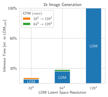
Figure 1: Comparison between 1k image synthesis using different architectures. We utilize SD V1.5 as our base model for LDM and scale the attention accordingly based on [22]. LDM’s inference time grows quadratically with higher resolutions, making real-time inference nearly impractical at a $128^{2}$ resolution latent space. In contrast, the integration of Coupling Flow Matching model (CFM) with $50$ function evaluations exhibits consistently faster inference, highlighting its efficiency in handling high-resolution image synthesis.

Visual synthesis has recently witnessed unprecedented progress and popularity in computer vision and beyond. Various generative models have been proposed to address the diverse challenges in this field [62], including sample diversity, quality, resolution, and training, and test speed. Among these approaches, diffusion models (DMs) [50, 47, 48] currently rank among the most popular and highest quality, defining the state of the art in numerous synthesis applications. While DMs excel in sample quality and diversity, they face challenges in high-resolution synthesis, slow sampling speed, and a substantial memory footprint.

		Closeup Roman statue ofaristoteles black and white made of marble,artstation award-winning, photorealistic Anime art of ghost in the shell,detailed scene, red, perfect face Viking ship sailing northeast, detailed, 8k
LCM (SDXL)	time per image: 0.408s
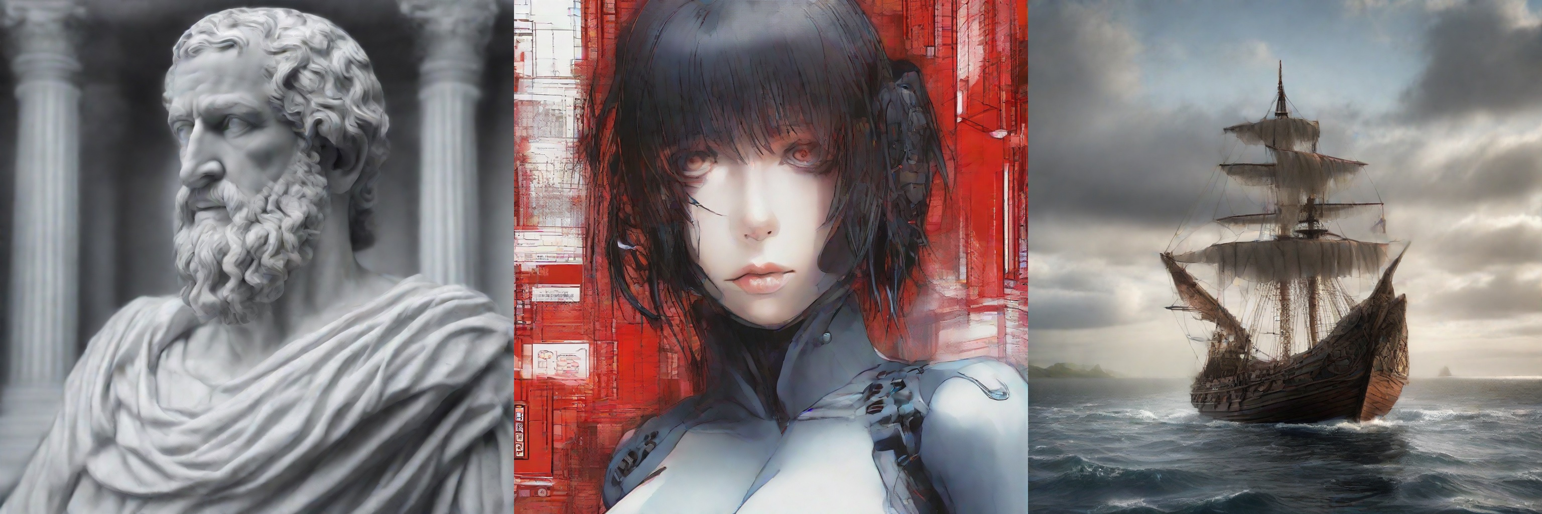
LCM (SD V1.5) + CFM (Ours)	time per image: 0.347s

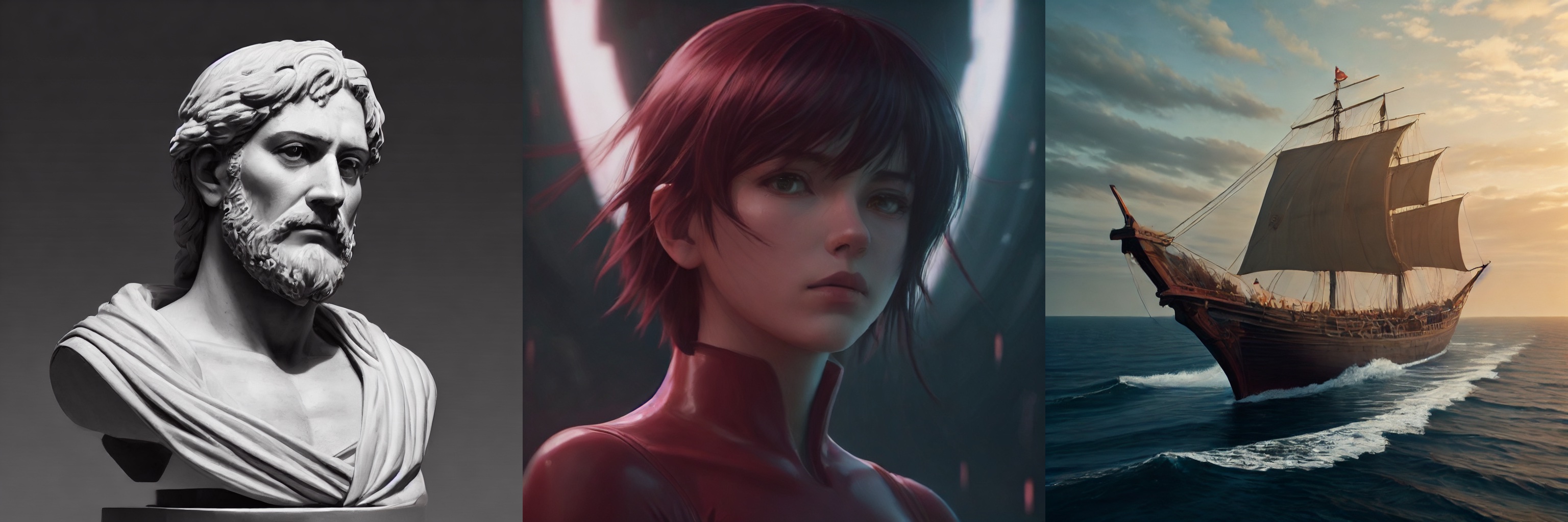
Figure 2: Samples synthesized in $1024^{2}$ px. We elevate DMs and similar architectures to a higher-resolution domain, achieving exceptionally rapid processing speeds. We leverage the Latent Consistency Models (LCM) [39], distilled from SD V1.5 [48] and SDXL [44] respectively. To achieve the same resolution as LCM(SDXL), we boost LCM(SD V1.5) with our general Coupling Flow Matching (CFM) model. This yields a further speedup in the synthesis process and enables the generation of high-resolution images of high fidelity in average $0.347$ seconds. The LCM(SDXL) model fails to produces competitive results within this shortened timeframe, highlighting the effectiveness of our approach in achieving both speed and quality in image synthesis.

Lately, numerous efficiency improvements to DMs have been proposed [10, 57, 46], but the most popular remedy has been the introduction of Latent Diffusion Models (LDMs) [48]. Operating only in a compact latent space, LDMs combine the strengths of DMs with the efficiency of a convolutional encoder-decoder that translates the latents back into pixel space. However, Rombach et al. [48] also showed that an excessively strong first-stage compression leads to information loss, limiting generation quality. Efforts have been made to expand the latent space [44] or stack a series of different DMs, each specializing in different resolutions [50, 19], but these approaches are still computationally costly, especially when synthesizing high-resolution images.

The inherent stochasticity of DMs is key to their proficiency in generating diverse images. In the later stages of DM inference, as the global structure of the image has already been generated, the advantages of stochasticity diminish. Instead, the computational overhead due to the less efficient stochastic diffusion trajectories becomes a burden rather than helping in up-sampling to and improving higher resolution images [7]. At this stage, converse characteristics become beneficial: reduced diversity and a short and straight trajectory towards the high-resolution latent space of the decoder. These goals align precisely with the strengths of Flow Matching (FM) [32], another emerging family of generative models currently gaining significant attention. In contrast to DMs, Flow Matching enables the modelling of an optimal transport conditional probability path between two distributions that is significantly straighter than those achieved by DMs, making it more robust, and efficient to train. The deterministic nature of Flow Matching models also allows the utilization of off-the-shelf ODE solvers, which are more efficient to sample from and can further accelerate inference.

We leverage the complementary strengths of DMs, FMs, and VAEs: the diversity of stochastic DMs, the speed of Flow Matching in training and inference stages, and the efficiency of a convolutional decoder when mapping latents into pixel space. This synergy results in a small diffusion model that excels in generating diverse samples at a low resolution. Flow Matching then takes a direct path from this lower-resolution representation to a higher-resolution latent, which is subsequently translated into a high-resolution image by a convolutional decoder. Moreover, the Flow Matching model can establish data-dependent couplings with the synthesized information from the DM, which automatically and inherently forms optimal transport paths from the noise to the data samples in the Flow Matching model [60, 5].

Note that our work is complementary to recent work on sampling acceleration of diffusion models like DDIM [57], DPM-Solver [37], and LCM-LoRA [38, 39]. Our approach can be directly integrated into any existing diffusion model architecture to efficiently increase the final output resolution.

2 Related Work

Diffusion Models Diffusion models [56, 18, 58] have shown broad applications in computer vision, spanning image [48], audio [33], and video [20, 8]. Albeit with high fidelity in generation, they do so at the cost of sampling speed compared to alternatives like Generative Adversarial Networks [15, 23, 25]. Hence, several works propose more efficient sampling techniques for diffusion models, including distillation [52, 59, 40], noise schedule design [27, 43, 45], and training-free sampling [57, 26, 36, 34]. Nonetheless, it is important to highlight that existing methods have not fully addressed the challenge imposed by the strong curvature in the sampling trajectory, which limits sampling step sizes and necessitates the utilization of intricately tuned solvers, making sampling costly.

Flow Matching-based Generative Models A recent competitor, known as Flow Matching [32, 35, 4, 41], has gained prominence for its ability to maintain straight trajectories during generation by modeling the synthesis process using an optimal transport conditional probability path with ordinary differential equations (ODE), positioning it as an apt alternative for addressing trajectory straightness-related issues encountered in diffusion models. The versatility of Flow Matching has been showcased across various domains, including image [32, 12, 21], video [6], audio  [28]. This underscores its capacity to address the inherent trajectory challenges associated with diffusion models, mitigating the limitations of slow sampling in the current generation based on diffusion models. Considerable effort has been directed towards optimizing transport within Flow Matching models [60, 35], which contributes to enhanced training stability and accelerated inference speed by making the trajectories even straighter and thus enabling larger sampling step sizes. However, the efficacy of Flow Matching in generation capabilities presently does not parallel that of diffusion models [32, 12].

This may be attributed to the presence of random noise within the training process as opposed to diffusion models, where it increases the stochasticity and flexibility of the generation process. In this paper, we remedy this limitation by incorporating a small diffusion model for synthesis quality.

Image Super-Resolution Image super-resolution (SR) is a fundamental problem in computer vision. Prominent methodologies include GANs [29, 61, 65, 23], diffusion models [64, 51, 30] and Flow Matching methods [32, 5].

Our methodology adopts the Flow Matching approaches, leveraging it’s objective to achieve faster training and inference compared to diffusion models. We take inspiration from latent diffusion models [48] and transition the training to the latent space, which further enhances computational efficiency. This enables the synthesis of images with significantly higher resolution, thereby advancing the capacity for image generation in terms of both speed and output size.

3 Method

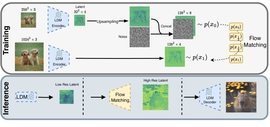
Figure 3: Approach overview. Top. During training we feed both a low- and a high-resolution image through the pre-trained Latent Diffusion Encoder to obtain a low- and a high-resolution latent code, respectively. In order to match the dimensionality we up-sample the low-resolution image with either bi-linear or nearest neighbor up-sampling. Depending on the model, we concatenate Gaussian noise and perform flow matching for a step $t\in[0,1]$ between the up-sampled low-resolution latent and the high-resolution latent. Bottom. During inference we can take any Latent Diffusion model that uses the same Encoder-Decoder architecture, generate the low-resolution latent, and then use the flow matching model to synthesize the higher dimensional latent code. Finally, the pre-trained decoder projects the latent code back to pixel space.

We speed up and increase the resolution of existing LDMs by integrating Flow Matching in the latent space. The proposed architecture should not be limited to unconditional image synthesis but also be applicable to text-to-image synthesis [48, 42, 50, 47] and Diffusion models with other conditioning including depth maps, canny edges, etc. [14, 66, 31].

The main challenge is not a deficiency in diversity within the Diffusion model; rather it is the slow convergence of the training procedure, the huge memory demand, and the slow inference [63, 44, 50]. While there are substantial efforts to accelerate inference speed of DMs either by distillation techniques [40], or by an ODE approximation at inference [57, 36, 37], we argue that we can achieve faster training and inference speed by training with an ODE assumption [32]. Flows characterized by straight paths without Wiener process inherently incur minimal time-discretization errors during numerical simulation [35] and can be simulated with only few ODE solver steps.

Outline Our solution to high-resolution image generation involves a small Diffusion model and a dedicated Flow Matching model. In Sec. 3.1, we explore the intricacies of the Diffusion model. Its reduced size can be strategically chosen to strike a balance between model complexity and performance, ensuring optimal proficiency in capturing complex data distributions. The Flow Matching model specializes in high-resolution image generation, which we will cover in Sec. 3.2. Finally, the combination of both methods is detailed in Sec. 3.3, illustrating the combination of the strengths of the Diffusion and Flow Matching models for comprehensive high-resolution image generation.

3.1 Diffusion Models

Diffusion models are likelihood-based probabilistic models that learn a data distribution $p(x)$ by reversing a fixed forward noising process. Starting with data samples $x_{0}$, a fixed Markov chain adds noise to it, creating increasingly noisy versions $x_{t}$,

$$q(x_{t}\mid x_{0})=\mathcal{N}(\alpha_{t}x_{0},\sigma_{t}^{2}\mathbf{I}),$$ (1)

where $\alpha_{t}$ and $\sigma^{2}_{t}$ are positive scalar-valued functions of timestep $t\in[0,T]$ that determine the signal-to-noise ratio of the noising process. The signal of $x_{0}$ is completely destroyed at timestep $T$ so that $x_{T}$ follows a standard Gaussian distribution with the same dimensionality as $x_{0}$. The training objective of Diffusion models is a reweighted variant of the variational lower bound on $p(x)$ [18],

$$L_{\text{simple}}(\theta):=\mathbb{E}_{t,x_{0},\epsilon\sim\mathcal{N}(0,\mathbf{I})}\Bigl{[}\lVert\epsilon-\hat{\epsilon}_{\theta}(x_{t},t)\rVert^{2}\Bigr{]},$$ (2)

where $\hat{\epsilon}_{\theta}$ is a function approximator that tries to model the reverse process noise at each intermediate step of the Markov chain, and $t$ is uniformly sampled in the range $[1,T]$ during training. During inference, $\hat{\epsilon}_{\theta}$ is used to iteratively denoise a Gaussian for $T$ steps until it finally arrives at a data sample $x_{0}\sim p(x)$.

The stochasticity inherent in Diffusion models enables them to effectively approximate the data manifold, even for high-dimensional complex data such as images  [50, 43] and videos [20, 54, 8]. However, to arrive at this high data variety, Diffusion models usually require a large number of training iterations on vast amounts of training data, making them inefficient for high-resolution images. To mitigate the problem and to foster high-resolution image synthesis, Rombach et al. [48] propose Latent Diffusion Models (LDMs). With a pre-trained Kullback-Leibler-regularized autoencoder, they perceptually compress images to a lower-dimensional latent space and perform Diffusion training in this space. Assuming an encoder $\mathcal{E}$, the objective from Eq. 2 can then be expressed as

$$L_{\text{LDM}}(\theta):=\mathbb{E}_{t,\mathcal{E}(x_{0}),\epsilon\sim\mathcal{N}(0,\mathbf{I})}\Bigl{[}\lVert\epsilon-\hat{\epsilon}_{\theta}(z_{t},t)\rVert^{2}\Bigr{]},$$ (3)

where $z_{t}$ refers to the encoded image noised to timestep $t$ with the forward noising process described in Eq. 1. The decoder $\mathcal{D}$ thereafter decompresses the latent $z_{0}$ back into pixel space.

LDMs exhibit multiple desirable properties: the stochastic formulation of Diffusion models allows us to model a large data diversity, generating an image’s global structure and semantics. The compression into latent space additionally reduces computational demands during training, whereas during inference, we can utilize the decoder to recover high-frequency details and the higher-resolution image from the generated latent. In combination, both provide for great diversity and fast training and inference. Nonetheless, compression with the autoencoder is limited so that stronger compression deteriorates quality [48].

From LDM to FM-LDM Hence, while the stochastic Diffusion model allows diverse sampling and the first stage compresses from pixel space into the latent space, we seek an orthogonal approach to model the straight trajectory from low-resolution to higher-resolution representations. Given the already generated semantics of an image from the Diffusion model, we claim that there is no need to utilize further stochastic processes to map to a higher dimensional space. Assuming a direct mapping, we propose modeling this part as a straight trajectory, which allows more efficient training and faster inference. Concretely, by letting Diffusion models focus only on semantic information, we can reduce their size and enhance the generation process with simpler, more lightweight models. Recently, the formulation of generative processes as optimal transport conditional probability paths has gained much attraction [4, 60, 32], perfectly suiting this task of modeling straight trajectories between two distributions.

3.2 Flow Matching

Flow Matching models are generative models that regress vector fields based on fixed conditional probability paths. Let $\mathbb{R}^{d}$ be the data space with data points $x$. Let $u_{t}(x):[0,1]\times\mathbb{R}^{d}\rightarrow\mathbb{R}^{d}$ be the time-dependent vector field, which defines the ODE in the form of $dx=u_{t}(x)dt$, and let $\phi_{t}(x)$ denote the solution to this ODE with the initial condition $\phi_{0}(x)=x$.

The probability density path $p_{t}:[0,1]\times\mathbb{R}^{d}\rightarrow\mathbb{R}_{>0}$ depicts the probability distribution of $x$ at timestep $t$ with $\int p_{t}(x)dx=1$. The pushforward function $p_{t}=[\phi_{t}]_{\#}(p_{0})$ then transports the probability density path $p$ along $u$ from timestep $0$ to $t$.

Assuming that $p_{t}(x)$ and $u_{t}(x)$ are known, and the vector field $u_{t}(x)$ generates $p_{t}(x)$, we can regress a vector field $v_{\theta}(t,x)$ parameterized by a neural network with learnable parameters $\theta$ using the Flow Matching objective

$$\mathcal{L}_{FM}(\theta)=\mathbb{E}_{t,p_{t}(x)}||v_{\theta}(t,x)-u_{t}(x)||.$$ (4)

While we generally do not have access to a closed form of $u_{t}$ because this objective is intractable, Lipman et al. [32] showed that we can acquire the same gradients and therefore efficiently regress the neural network using the conditional Flow Matching (CFM) objective, where we can compute $u_{t}(x|z)$ by efficiently sampling $p_{t}(x|z)$,

$$\mathcal{L}_{CFM}(\theta)=\mathbb{E}_{t,q(z),p_{t}(x|z)}||v_{\theta}(t,x)-u_{t}(x|z)||,$$ (5)

with $z$ as a conditioning variable and $q(z)$ the distribution of that variable. We parameterize $v_{\theta}$ as a U-Net [49], which takes the data sample $x$ as input and $z$ as conditioning information.

3.2.1 Gaussian Assumption

We first assume that the probability density path starts from $p_{0}$ with standard Gaussian distribution and ends up in a Gaussian distribution $\mathcal{N}(x_{1},\sigma_{\min}^{2})$ that is smoothed around a data sample $x_{1}$ with minimal variance. In this case, the conditioning signal $z$ would be $x_{1}$, and the optimal transportation path would be formulated as follows [32],

$$p_{t}(x|z)=\mathcal{N}(x|tx_{1},(t\sigma_{\min}-t+1)^{2}\mathbf{I}),$$ (6)

$$u_{t}(x|z)=\frac{x_{1}-(1-\sigma_{\min})x}{1-(1-\sigma_{\min})t},$$ (7)

$$\phi_{t}(x|z)=(1-(1-\sigma_{\min})t)x+tx_{1}.$$ (8)

The resulting CFM loss takes the form of

$$\begin{split}\mathcal{L}_{CFM}(\theta)&=\mathbb{E}_{t,z,p_{t}(x|z)}||v_{\theta}(t,\phi_{t}(x_{0}))-\frac{d}{dt}\phi_{t}(x_{0})||\\ &=\mathbb{E}_{t,z,p(x_{0})}||v_{\theta}(t,\phi_{t}(x_{0}))-(x_{1}-(1-\sigma_{\min})x_{0})||.\end{split}$$ (9)

3.2.2 Data-Dependent Couplings

In our case, we also have access to the representation of a low-resolution image generated by a Diffusion model at inference time. It seems then intuitive to incorporate the inherent relationship between the conditioning signal and our target within the Flow Matching objective, as is also stated in [5]. Let $x_{1}$ denote a high-resolution image data sample. The conditioning signal $z:=x_{1}$ remains unchanged from the previous formulation. Instead of randomly sampling from a Gaussian distribution in the naïve Flow Matching method, the starting point $x_{0}=\mathcal{E}(x_{1})$ corresponds to an encoded representation of the image, with $\mathcal{E}$ being a fixed encoder.

Like in the previously described case, we smooth around the data samples within a minimal variance to acquire the corresponding data distribution $\mathcal{N}(x_{0},\sigma_{\min}^{2})$ and $\mathcal{N}(x_{1},\sigma_{\min}^{2})$. The Gaussian flows can be defined by the equations

$$p_{t}(x|z)=\mathcal{N}(x|tx_{1}+(1-t)x_{0},\sigma_{\min}^{2}\mathbf{I}),$$ (10)

$$u_{t}(x|z)=x_{1}-x_{0},$$ (11)

$$\phi_{t}(x|z)=tx_{1}+(1-t)x_{0}.$$ (12)

Notably, the optimal transport condition between the probability distributions $p_{0}(x|z)$ and $p_{1}(x|z)$ is inherently and automatically satisfied due to the low-resolution high-resolution data coupling. This automatically solves the dynamic optimal transport problem in the transition from low to high resolution within the Flow Matching paradigm, enabling more stable and faster training [60]. We name these Flow Matching models with data-dependent couplings Coupling Flow Matching (CFM) models, and the CFM loss then takes the form of

$$\mathcal{L}_{CFM}(\theta)=\mathbb{E}_{t,z,p(x_{0})}||v_{\theta}(t,\phi_{t}(x_{0}))-(x_{1}-x_{0})||.$$ (13)

Note that the encoder $\mathcal{E}$ can be generalized to a wide range of image representations with spatial information, including but not limited to perceptual image compression [48], semantic segmentation maps [9] and more.

3.2.3 Noise Augmentation

Noise Augmentation is a technique for boosting generative models’ performance introduced for cascaded Diffusion models [19]. The authors found that applying random Gaussian noise or Gaussian blur to the conditioning signal in super-resolution Diffusion models results in higher-quality results during inference. Drawing inspiration from this, we also implement Gaussian noise augmentation on $x_{0}$. Following the notation from variance-preserving DMs, we noise $x_{0}$ according to the cosine schedule first proposed in [43]. In line with [19], we empirically discover in our experiments that incorporating a specific amount of Gaussian noise enhances performance. We hypothesize that including a small amount of Gaussian noise smoothes the base probability density $p_{0}$ so that it remains well-defined over the higher-dimensional space. Note that this noise augmentation is only applied to $x_{0}$ but not to the conditioning information $z$, since the model relies on the precise conditioning information to construct the straight path.

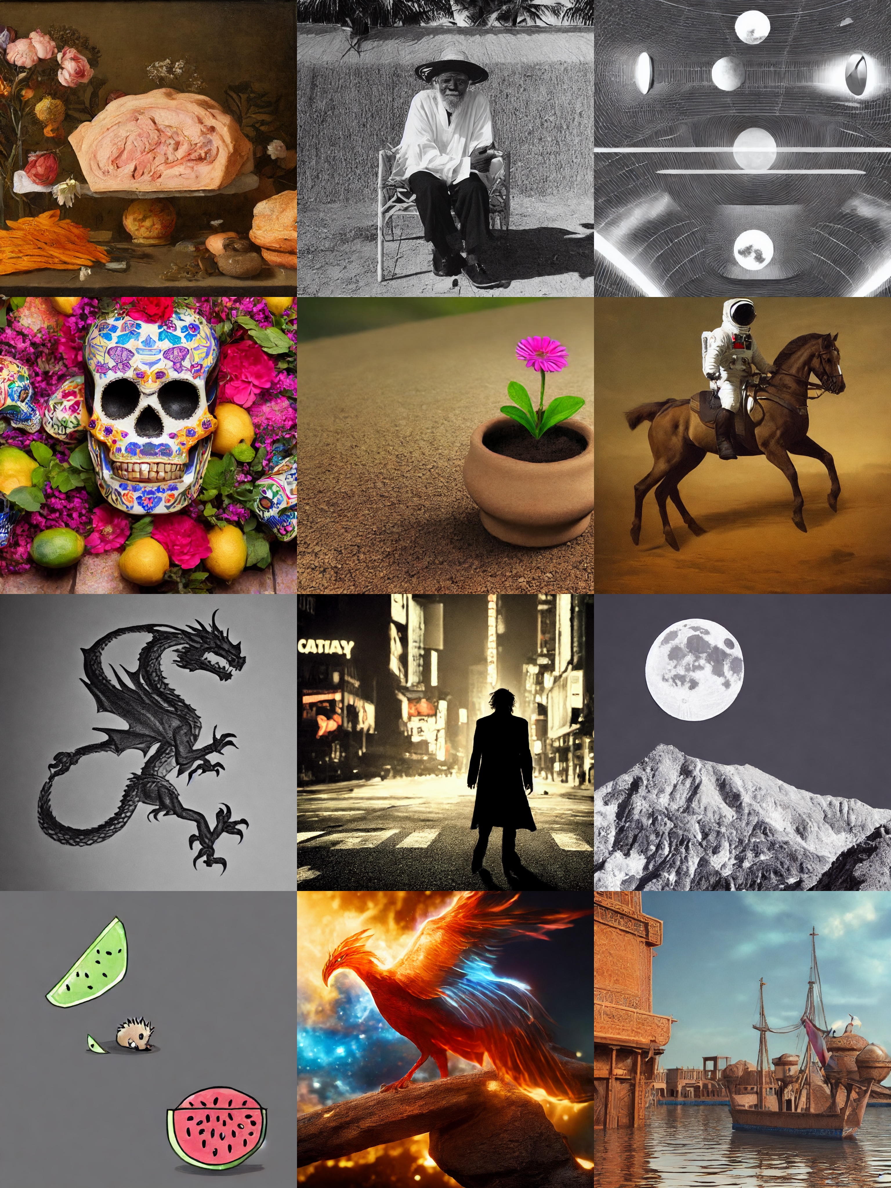
Figure 4: Uncurated samples from the Coupling Flow Matching model on top of Stable Diffusion V1.5 [48] using a classifier-free guidance scale of $7.5$. Samples are generated in latent space $64^{2}$ and up-sampled with CFM from $64^{2}$ to $128^{2}$. The resulting images have a resolution of $1024\times 1024$.

3.2.4 Latent Flow Matching

In order to reduce the computational demands associated with training Flow Matching models for high-resolution image synthesis, we take inspiration from [48, 12] and utilize an autoencoder model that provides a compressed latent space that aligns perceptually with the image pixel space similar to LDMs. By training in the latent space, we get a three-fold advantage: i) The computational cost associated with the training of Flow Matching models is reduced substantially, thereby enhancing the overall efficiency of the training process. ii) Leveraging the latent space unlocks the potential to synthesize images with significantly increased resolution efficiently. iii) The lower resolution in the latent space also yields quicker inference speed in the synthesis task.

3.3 High-Resolution Image Synthesis

Overall, our approach integrates all the components discussed above into a cohesive synthesis pipeline, as depicted in detail in Fig. 3. We start from a DM for content synthesis and move the generation to a latent space with a pretrained VAE encoder, which optimizes memory usage and enhances inference speed. To further alleviate the computational load of DM and achieve additional acceleration, we adopt a relatively compact DM that produces compressed information. Subsequently, the FM model projects the compressed information to a high-resolution latent image with a straight conditional probability path. Finally, we decompress the latent space using a pretrained VAE decoder. Note that the VAE decoder performs well across various resolutions, as we demonstrate in Fig. 16 and Tab. 6 in the supplementary materials.

The integration of FM with DMs in the latent space presents a promising approach to address the trade-off between flexibility and efficiency in modeling the dynamic image synthesis process. The inherent stochasticity within a DM’s sampling process allows for a more nuanced representation of complex phenomena, while the FM model exhibits greater computational efficiency, which is useful when handling high-resolution images, but lower flexibility and image fidelity as of yet when it comes to image synthesis [32]. By combining them in the pipeline, we benefit from the flexibility of the DM while capitalizing on the efficiency of FM as well as VAE.

4 Experiments

Combining a diffusion synthesis model and a flow matching super-resolution model yields great synthesis capability in the high-resolution domain, as we show qualitatively and quantitatively in this section. We first demonstrate the effectiveness of the combination, and then provide an extensive ablation and analysis of our CFM model. Subsequently, we assess our model in comparison to the current state-of-the-art diffusion approach.

4.1 Datasets

The general dataset that we use for training and ablations is FacesHQ, a compilation of CelebA-HQ [24] and FFHQ [25], as employed in previous work such as [13]. This dataset serves as a foundation for evaluating various aspects of our model. We also include ablations on LHQ [55], which contains 90k high-resolution landscape images.

For the general flow matching (FM) model, particularly targeted towards combination with latent diffusion models, we utilize the Unsplash dataset [3], which provides diverse and high-quality images for training our model. We present inference results of our general FM model on a high-resolution subset of LAION 5B [53].

4.2 Boosting LDM with FM

Aggregating the power of LDM and FM results in remarkable performance in image synthesis. Combining the flexibility of LDM with the intrinsic characteristics of FM achieves an optimal trade-off between computational efficiency and visual fidelity.

Since LDMs are typically trained and evaluated on fixed sizes, we follow [22] and apply attention scaling on SD to synthesize images of varying resolutions. We also finetune the small LDM model which outputs images at resolutions of $256^{2}$ px to further ensure image fidelity. More details can be found in Appendix Sec. 6.2. We plot the inference speed for $1024^{2}$ px image in Fig. 1, where we visualize the time taken by LDM and FM distinctively. Note that the LDM’s inference time scales quadratically with increasing resolution, and the inference is almost impractical for a real-time inference for a latent space of $128^{2}$. Conversely, the CFM model shows remarkably fast inference speed, which emphasises the efficiency improvements achieved by its integration for high-resolution image synthesis.

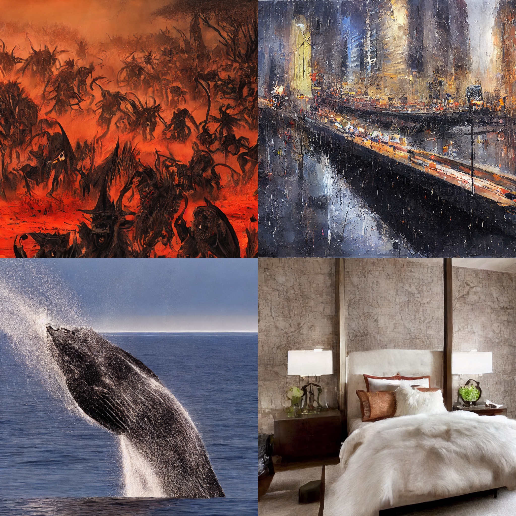
Figure 11: Samples from the Coupling Flow Matching model on top of Stable Diffusion V1.5 [48] using a classifier-free guidance scale of $7.5$. Samples are generated in latent space $64^{2}$ and up-sampled with CFM from $64^{2}$ to $128^{2}$. The resulting image has a resolution of $1024\times 1024$. Best viewed when zoomed-in.

We demonstrate the models’ synthesized image quality in Fig. 5. Both combinations of LDM and FM surpass the performance of the attention-scaled LDM-128 baseline in terms of inference time and image quality. The intermediate resolution of $32^{2}$ yields faster inference, while the intermediate resolution of $64^{2}$ maintains better image fidelity. Note that we achieve near-optimal results with as few as $10$ ODE steps for the CFM model, which adds minimal computational overhead to the underlying DM. Note that we selectively use a subset of $1$k samples from LAION to highlight variations in NFE for a fair comparison across all models. This choice is for rapid evaluation purposes, and the FID is expected to decrease with a larger sample size. We present a selection of image samples of LDM-64 and CFM $64^{2}\rightarrow 128^{2}$ in Fig. 4. Please refer to Fig. 11 and Fig. 14 in the Appendix for more samples.

We also investigate the results for consistency models [59], which significantly accelerate the inference process by distilling information from a diffusion model. The LCM-LoRA model [39] finetuned on SD V1.5 [48] produces $512\times 512$ resolution images. We can further improve this model to 1k resolution images with our CFM model. We present our synthesised results in Fig. 2. The inference time for a batch of four samples is $1.388$ seconds. The LCM-LoRA SDXL model [44] fails to produce images with similar fidelity at the same resolution in the same time range.

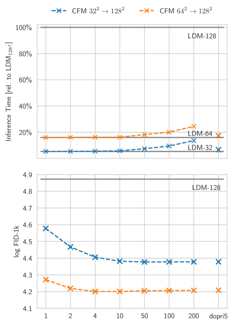
Figure 5: Inference time per model part (LDM or CFM) and FID for synthesizing images with resolution $1024\times 1024$ for different number of function evaluations (NFE). The upper plot refers to the average inference time relative to LDM-128, while the lower plot indicates $\log$ FID for $1$k samples. dopri5 corresponds to the Dormand-Prince adaptive step-size solver. For LDM-128 we do not use any CFM model.

4.3 FM Model Ablation

Upsampling Methods As our flow matching model requires that $x_{0}$ and $x_{1}$ share the same dimensionality, we need to upsample the latent code. In this context, we conduct an ablation study comparing two upsampling methods: nearest neighbor and bi-linear upsampling. The results are presented in Tab. 1. While the choice between these methods does not appear to be decisive based on SSIM and PSNR metrics, we observe generally lower FID [16] values with nearest neighbor upsampling.

	CelebA-HQ			FFHQ			FacesHQ
Model	SSIM $\uparrow$	PSNR $\uparrow$	FID $\downarrow$	SSIM $\uparrow$	PSNR $\uparrow$	FID $\downarrow$	SSIM $\uparrow$	PSNR $\uparrow$	FID $\downarrow$
CFM-nearest	0.75	26.47	4.00	0.70	25.47	3.65	0.72	25.80	2.75
CFM-bilinear	0.75	26.43	4.58	0.70	25.50	3.94	0.70	25.49	3.93
FM-nearest	0.75	26.47	7.91	0.70	25.47	8.16	0.71	25.80	6.84
FM-bilinear	0.75	26.47	8.10	0.69	25.47	7.98	0.71	25.80	6.78

Table 1: Ablation of up-sampling methods for Flow Matching in the latent space. While the choice between these methods does not appear to be decisive based on SSIM and PSNR metrics, we observe generally lower FID values with nearest neighbor upsampling which also matches the visual inspection of generated results shown in the supplementary.

LR
Reg
FM
CFM

Figure 6: Results of different latent space up-sampling strategies from $32\times 32$ to $128\times 128$. LR corresponds to bilinear upsampling of the low-resolution image, Reg refers to the regression baseline. FM and CFM correspond to Flow Matching and Coupling Flow Matching with a noising step of 400, respectively.

GT	REG	LR	FM

Figure 7: Qualitative comparison of the Flow Matching (FM) model to the upsampled low resolution image (LR) the regression model (REG) and the ground truth (GT) using zoomed-in patches. The FM patches are significantly sharper and display more fine-grained structure and details.

	CelebA-HQ			FFHQ			FacesHQ
Model	SSIM $\uparrow$	PSNR $\uparrow$	FID $\downarrow$	SSIM $\uparrow$	PSNR $\uparrow$	FID $\downarrow$	SSIM $\uparrow$	PSNR $\uparrow$	FID $\downarrow$
Reg	0.81	26.99	56.15	0.77	26.29	48.22	0.78	26.52	48.32
FM	0.75	26.47	07.91	0.70	25.47	08.16	0.71	25.80	06.84
CFM	0.75	26.47	04.00	0.70	25.47	03.65	0.72	25.80	02.75

Table 2: Metric results for regression (Reg), Flow Matching (FM), and Coupling Flow Matching (CFM) corresponding to Fig. 6.

Flow Matching and Coupling Flow Matching In this ablation study, we systematically explore two variations of Flow Matching models – one incorporating the Gaussian assumption (FM) and the other incorporating data-dependent coupling (CFM). We evaluated these two variants quantitatively (Tab. 1) and qualitatively (Fig. 7), where we observed that the CFM models with data-dependent coupling readily outperform the ones without. We provide more information about the noise augmentation process in Tab. 3. Notably, in the specific upsampling scenario from $256^{2}$ to $1024^{2}$, we observe an optimal configuration with a noising timestep of 200. The introduction of Gaussian noise proves beneficial as it imparts a smoothing effect on the input probability path, resulting in improved performance. However, excessive Gaussian noise can lead to the loss of valuable information, subsequently deteriorating the data-dependent coupling and reverting the model’s behavior to the Gaussian assumption. This finding underscores the delicate balance required in incorporating noise for optimal model performance.

Intermediate Results along the ODE Trajectory Fig. 8 shows intermediate results along the ODE trajectory. It can be seen that the CFM model gradually transforms the image representation from one with grid artefacts due to nearest neighbour upsampling to its high-resolution image counterpart.

	CelebA-HQ			FFHQ			FacesHQ
Model	SSIM $\uparrow$	PSNR $\uparrow$	FID $\downarrow$	SSIM $\uparrow$	PSNR $\uparrow$	FID $\downarrow$	SSIM $\uparrow$	PSNR $\uparrow$	FID $\downarrow$
CFM-100	0.71	25.30	8.27	0.73	26.14	5.84	0.75	26.41	5.47
CFM-200	0.75	26.39	3.90	0.70	25.48	3.14	0.72	25.78	2.38
CFM-400	0.75	26.47	4.00	0.70	25.47	3.65	0.72	25.80	2.75
CFM-600	0.75	26.51	5.18	0.70	25.52	5.14	0.72	25.85	4.04
CFM-999	0.74	26.36	7.72	0.69	25.35	7.53	0.71	25.69	6.38

Table 3: Quantative evaluation on different noising steps for coupling flow matching (CFM) for $4\times$ upsampling from $256^{2}$ to $1024^{2}$ px. We evaluate the FID on the full dataset (5k, 10k, and 15k samples respectively).

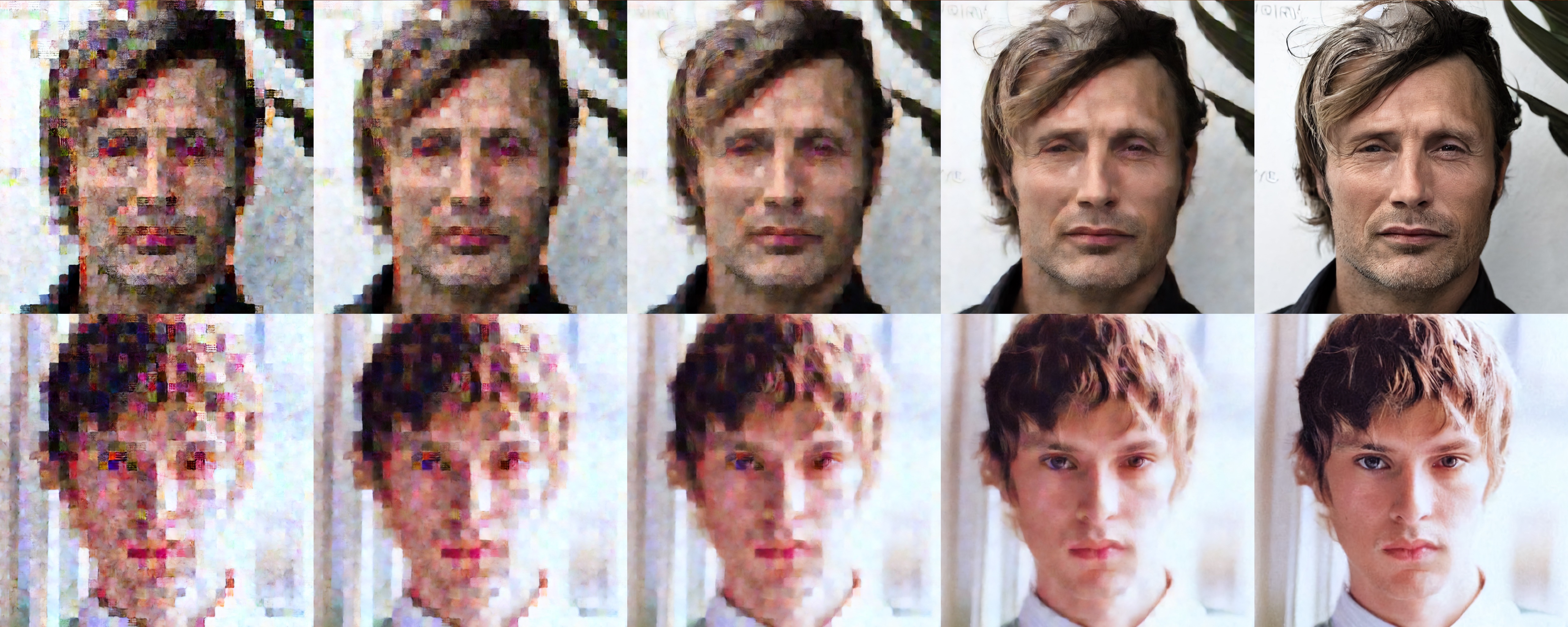
Figure 8: Intermediate results along the ODE trajectory with Euler ODE solver and $100$ function evaluations. From left to right, the number of function evaluations is $0\text{ (upsampled latent w/o FM)},25,50,75,\text{and }100.$

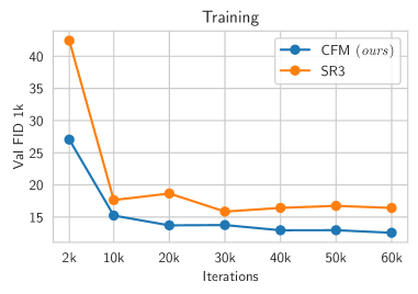
Figure 9: Comparison of diffusion-based SR3 [51] and our Coupling Flow Matching (CFM) over the training for $4\times$ up-sampling of the latent codes from $32^{2}\rightarrow 128^{2}$. Decoded output resolution is $1024^{2}$. Architecture and hyperparameters are kept fixed for both. FID evaluated on $1$k samples from the validation set. We use DDIM sampling with $50$ steps for the diffusion-based model and the Euler ODE solver with $50$ steps for CFM.

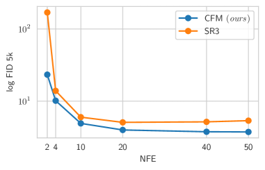
Figure 10: Comparison of diffusion-based SR3 [51] and our Coupling Flow Matching (CFM) for different number of function evaluations (NFE) for $4\times$ up-sampling of the latent codes from $32^{2}\rightarrow 128^{2}$. Decoded output resolution is $1024^{2}$. Architecture and hyperparameters are kept fixed for both. FID evaluated on $5$k samples from the validation set. We use DDIM [57] for diffusion-based sampling and the Euler ODE solver for the CFM model.

4.4 Comparison to Baselines

We compare our Coupling Flow Matching method to the diffusion-based up-sampling method SR3 [51], as well as a simple regression baseline, trained with a simplep $L2$ loss, on the FacesHQ dataset. For a fair comparison, we keep the architecture and hyperparameters fixed for all three models. We obtain the latent codes by using the pre-trained KL-regularized autoencoder from [48] and perform nearest neighbor up-sampling to fit the dimensionality of our starting condition $x_{0}$.

Upsampling Results

Fig. 6 shows results of different latent space up-sampling strategies from $32^{2}$ to $128^{2}$, increasing the final output resolution from $256^{2}$ to $1024^{2}$. We can observe that the simple regression baseline yields blurry results, which is also reflected in the metrics (see Tab. 2). In contrast, both flow matching approaches – Coupling Flow Matching (CFM) and Flow Matching starting from a noise distribution (FM) – yield better results. Also, metric-wise, both outperform the simple regression baseline by a large margin. When directly comparing the low-resolution image at size $256^{2}$ with the decoded output of our Flow Matching model (Fig. 6), we can observe that FM adds fine-grained details to the image not visible in the lower-resolution counterpart.

Training Efficiency

Based on optimal transport theory, the training of a constant velocity field presents a more straightforward training objective when contrasted with the intricate high-curvature probability paths found in diffusion models [32, 12]. This distinction often translates to slower training convergence and potentially sub-optimal trajectories for DMs, which could detrimentally impact both, training duration and overall model performance. Fig. 9 shows the FID over the course of training for the diffusion-based SR3 and our Flow Matching model. We can clearly observe that the Flow Matching model achieves a lower FID more rapidly and produces superior results, compared to the SR3 model. Fig. 10 further demonstrates that after $100$k iterations and for different number of function evaluations (NFE), we consistently attain a lower FID compared to the diffusion-based SR3 model. Taken together, these findings underscore the training efficiency of Flow Matching over Diffusion models and its superior performance for the up-sampling task.

5 Conclusion

Our work introduces a novel and effective approach to high-resolution image synthesis, combining the generation diversity of Diffusion Models, the efficiency of Flow Matching, and the effectiveness of convolutional decoders. Strategically integrating Flow Matching models between a standard latent Diffusion model and the convolutional decoder enables a significant reduction in the computational cost of the generation process by letting the expensive Diffusion model operate at a lower resolution and up-scaling its outputs using an efficient Flow Matching model. Our Flow Matching model efficiently enhances the resolution of the latent space without compromising quality. Our approach complements DMs with their advancements and is orthogonal to their recent enhancements such as sampling acceleration and distillation techniques e.g., LCM [39]. This allows for mutual benefits between different approaches and ensures the smooth integration of our method into existing frameworks.

Supplementary Material

We initiate our analysis by ablations on the flow matching model, systematically exploring its individual components and assessing their impact on the overall performance. Subsequently, we delve into a comprehensive examination of the combined effects of the flow matching and diffusion models. This examination considers both image quality and the efficiency gains achieved through this integration.

6 Quantitative Experimental Results

6.1 Discussion on Flow Matching

Effects of ODE Solver Steps on Image Quality We use the torchdiffeq [11] library for ordinary differential equation (ODE) solvers implemented in PyTorch. Tab. 4 demonstrates the ability of our flow matching model to produce strong results based on FID with as few as 10 function evaluations with additional speedups when compared against diffusion models. This highlights the efficiency and advantage of Flow Matching models in contrast to score-based models, which typically require more function evaluations due to its inherent stochasticity. Fig. 12 shows the average time needed for up-sampling a latent code from $32\times 32$ to $128\times 128$ on a single NVIDIA A100 GPU with batch-size of $4$ and Coupling Flow Matching. At 10 steps, the FID score plateaus, emphasizing the minimal gains from additional steps and empirically demonstrating that modeling direct trajectories accelerates sampling speed.

	FacesHQ-1k
NFE	SSIM $\uparrow$	PSNR $\uparrow$	FID $\downarrow$	Time $(s)$ $\downarrow$
1	0.81	27.41	66.24	0,395
2	0.81	27.86	33.89	0,399
4	0.79	27.71	17.69	0,413
10	0.78	27.10	11.53	0,465
50	0.75	26.50	10.31	0,718
100	0.75	26.50	10.30	1,046
1000	0.75	26.32	10.28	7,061
dopri5	0.75	26.31	10.34	0,996

Table 4: We ablate the CFM-200 model and compare different number of function evaluations (NFE) during inference for the Euler method, as well as the adaptive step-size Dormand-Prince solver. We evaluate the results on a subset of 1k samples of FacesHQ and present the total inference time on a single NVIDIA A100 GPU.

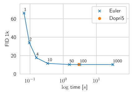
Figure 12: Average computation time on a single NVIDIA A100 GPU with batch-size $4$ for different number of function evaluations with the Euler method and the Dormand-Prince adaptive step-size ODE solver on the FacesHQ dataset.

We additionally illustrate the outcomes of image up-sampling for various number of function evaluations (NFE) in Fig. 13. An intriguing observation emerges when working with an exceptionally low NFE, which leads to higher PSNR and SSIM but with a notably increased blurriness. These results highly resemble the regression baseline model. With increasing number of steps images get sharper, with marginal to no perceptual differences between $10$ and $50$ NFEs. This again emphasizes the low number of function evaluations required to obtain reasonable high-resolution results from low-resolution conditioning information.

GT	NFE=1	NFE=2	NFE=4	NFE=10	NFE=50

Figure 13: Sample quality of different ODE solvers and different number of function evaluations (NFE). From left to right, 1st column represents the ground truth, high-resolution images. From 2nd column on, we show the results for NFE $={1,2,4,10,50}$ with the Euler fixed step-size ODE solver.

6.2 DMs for lower Resolutions

To evaluate the performance of our approach, we perform flow matching on also low-dimensional latents. The standard SD V1.5 [48] was trained to work on latents with a dimensionality of $64^{2}$ pixels. After decoding the latent, this results in generated images with a resolution of $512^{2}$ pixels. Sampling latents of a different dimensionality is also possible but results in degraded performance, which is particularly pronounced for sampling lower-resolution latents. This deterioration can be partially mitigated by changing the scale of the self-attention layers from the standard $\sqrt{1/d}$ to $\sqrt{\log_{T}N/d}$ where $d$ is the inner attention dimensionality and $T$ and $N$ the number tokens during the training and inference phase respectively [22]. We use this to rescale the attention layers of SD V1.5 for $32^{2}$ latents. Additionally, we finetune it on images of LAION-Aesthetics V2 6+ [1] rescaled to $256^{2}$ pixels for one epoch, a learning rate of $1e{-5}$, and batch size of $256$.

We provide fine-tuned LDM metrics on the LAION dataset in Tab. 5. We found that FID pleataus with a classifier-free guidance scale at $7.0$. Consequently, we adopt this value for small resolution ($32^{2}$ in the latent space), text-guided image synthesis. We illustrate the uncurated samples for the upsampled images in Fig. 14.

CFG	FID $\downarrow$	CLIP $\uparrow$
1	41.95	0.157
3	17.13	0.214
5	14.03	0.231
7	13.47	0.239
9	13.50	0.243

Table 5: Results of our fine-tuned Latent Diffusion Model on the LAION dataset for different Classifier-free guidance scales. [17]

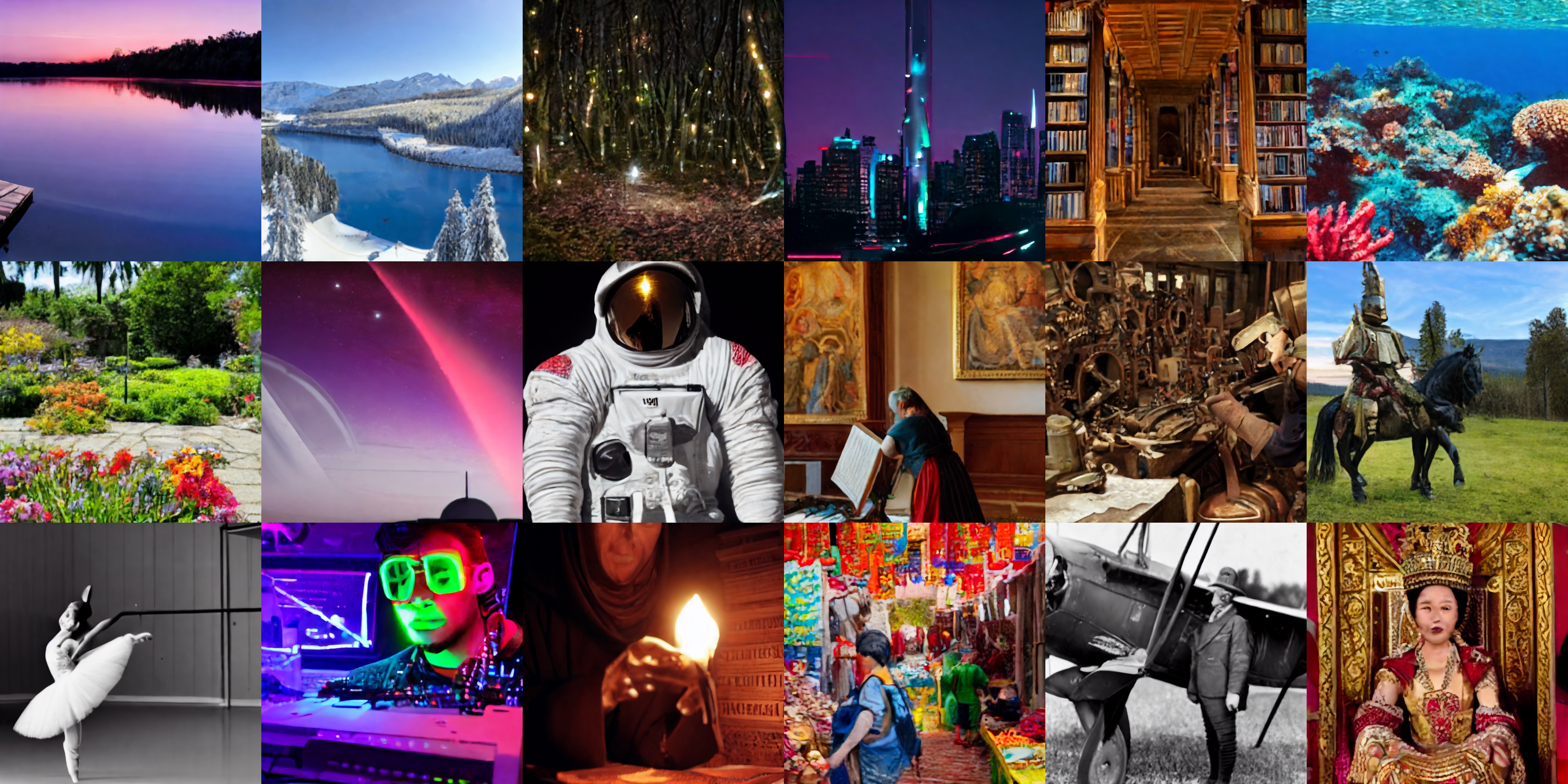
Figure 14: Uncurated samples from the Coupling Flow Matching model on top of finetuned Stable Diffusion for lower resolution using a classifier-free guidance scale of $7.0$. Samples are generated in latent space $32^{2}$ and up-sampled with CFM from $32^{2}$ to $128^{2}$. The resulting images have a resolution of $1024\times 1024$.

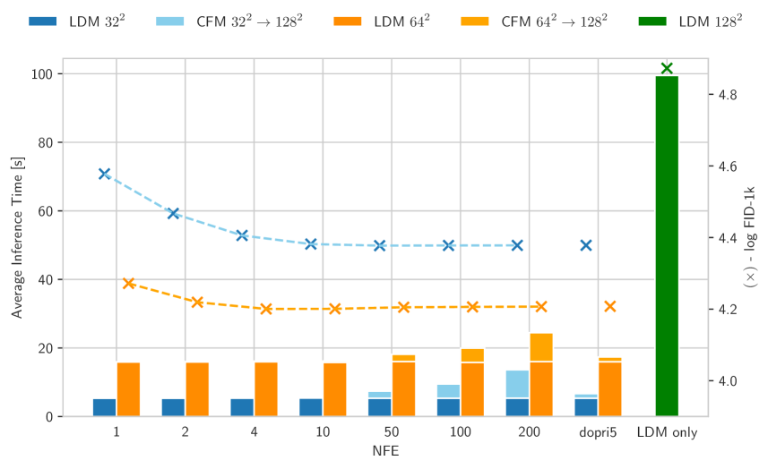
Figure 15: Absolute inference time per model part (LDM or CFM) and FID for synthesising images with resolution $1024\times 1024$ for different number of function evaluations (NFE). Left axis refers to average inference time in seconds, right axis to $\log$ FID for $1$k samples. Dopri5 corresponds to the Dormand-Prince adaptive step-size solver. For LDM $128^{2}$ we do not use any CFM model.

7 Qualitative Experimental Results

Fig. 18 shows additional, zoomed in results of our FacesHQ Coupling Flow Matching model, where we up-sample the latent code of $256^{2}$ images from $32^{2}$ to $128^{2}$ with the Dormand-Prince ODE solver. In Fig. 19 and Fig. 20 we visualize more, non-curated results from our Coupling Flow Matching model on the FacesHQ dataset and the LHQ dataset respectively.

Fig. 17 show generated text-to-image samples in $2048^{2}$ px using the LDM together with CFM up-sampling in latent space with an intermediate resolution of $512^{2}$, produced by SD V1.5.

8 Architecture and Implementation Details

In our implementation of FM, we follow Tong et al. [60] and set the minimal variance either as $\sigma_{\min}=1e{-8}$ or $\sigma_{\min}=1e{-4}$. We employ the cosine noising schedule [43] for noise augmentation [19], and $t\in[1,999]$ resembles the corresponding timestep. We adopt the widely used U-Net architecture as implemented in the OpenAI GitHub repository [2]. Implementation details and parameterization for the UNet used for our Coupling Flow Matching models can be found in Tab. 8.

KL Autoencoder

We employ the KL-regularized autoencoder from Stable Diffusion V1.5 [48] to compress images to their respective latent representations. We also shed light on how well the pre-trained autoencoder from Stable Diffusion perform on smaller and larger resolution. We focus here on the autoencoder architecture that we employ for latent compression, since it is crucial to ensure that the latent space captures perceptual information at various resolution. Thanks to the convolutional nature, the autoencoder exhibits the capability to encode images at multiple scales. To systematically evaluate its effectiveness, we present results using metrics such as FID, PSNR, and SSIM for images of different sizes. The detailed metrics are presented in Tab. 6, and the FID is calculated with a representative sample size of $10,000$ images. Fig. 16 additionally shows visual results. Our analysis underscores the autoencoder’s proficiency across multiple resolutions. Despite potential shortcomings in low-resolution compression, we contend that the FM model can adeptly learn to transition from this distribution to the latent space of the high-resolution image, thereby mitigating deficiencies in low-resolution performance.

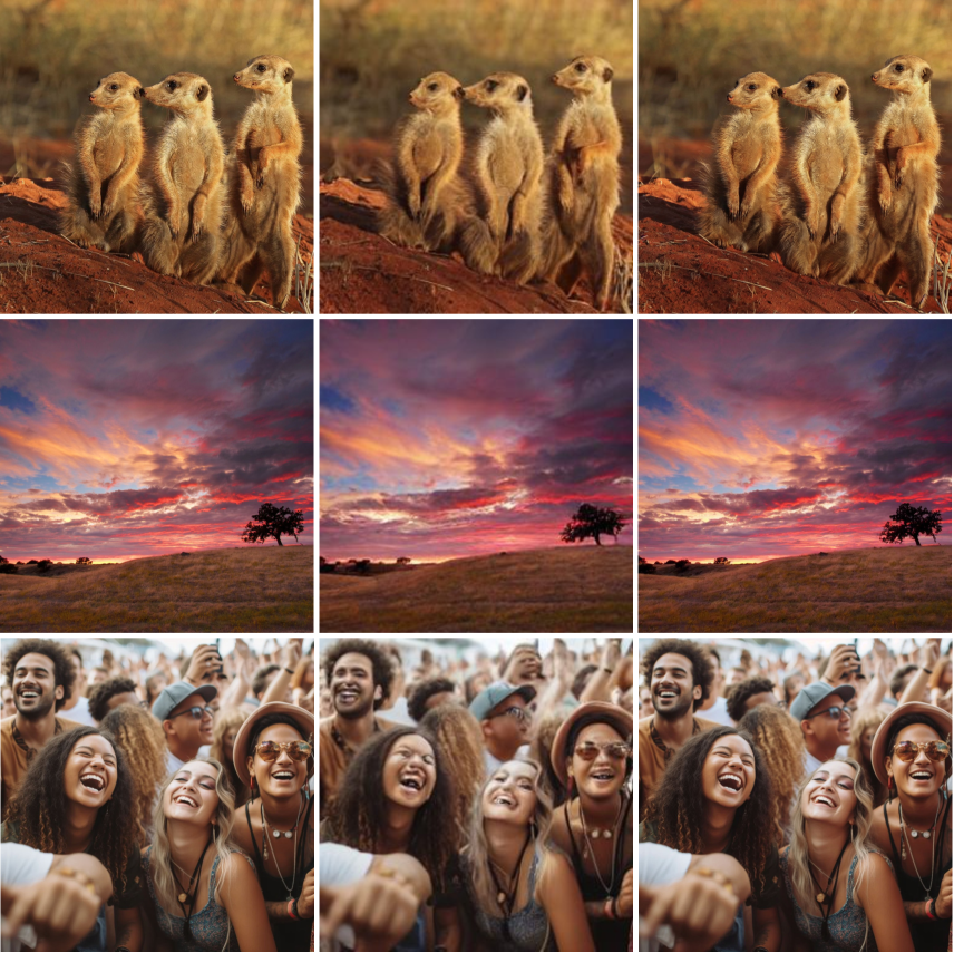
Figure 16: Comparison between reconstructed images (middle $256^{2}$ and right column $2048^{2}$) and their high-resolution original input (left column) using the pre-trained autoencoder. We can observe that the (i) pre-trained autoencoder is able to encode and decode images at different scales. (ii) It cannot reconstruct faces correctly in low resolution. (iii) The artifacts diminish with a higher resolution. Best viewed when zoomed in.

	LAION-10k
Image Size	SSIM $\uparrow$	PSNR $\uparrow$	FID $\downarrow$
256	0.82	26.42	2.47
512	0.86	28.65	1.28
1024	0.88	30.72	0.84
2048	0.88	32.20	0.60

Table 6: Evaluation of the pre-trained autoencoder performance under different image sizes.

	Big (306M)			Small (113M)
Model	SSIM $\uparrow$	PSNR $\uparrow$	FID $\downarrow$	SSIM $\uparrow$	PSNR $\uparrow$	FID $\downarrow$
FM	0.59	22.90	11.22	0.59	22.84	10.90
CFM-400	0.59	22.72	6.30	0.59	22.87	6.38
CFM-200	0.60	22.98	4.92	0.60	23.02	5.20

Table 7: LHQ ablation for $256^{2}\rightarrow 1024^{2}$ super-resolution results.

	FacesHQ	Unsplash	LHQ
Autoencoder $f$	8	8	8
$z$-shape	$4\times 64\times 64$	$4\times 64\times 64$	$4\times 64\times 64$
Model size	113M	306M	306M
Channels	128	128	128
Depth	3	3	3
Channel multiplier	1, 2, 3, 4	1, 2, 4, 8	1, 2, 4, 8
Attention resolutions	16	16	16
Head channels	64	64	64
Number of heads	4	4	4
Optimizer	Adam	Adam	Adam
Batch size	96	768	128
Learning rate	1e-4	1e-4	1e-4

Table 8: Hyperparameters and number of parameters for our FMs and DMs. We use the exact same architecture for our FM and the SR3 [51] upsampling model to ensure a fair comparison. We trained the SR3 model with $1000$ diffusion steps and a cosine noise schedule [43].

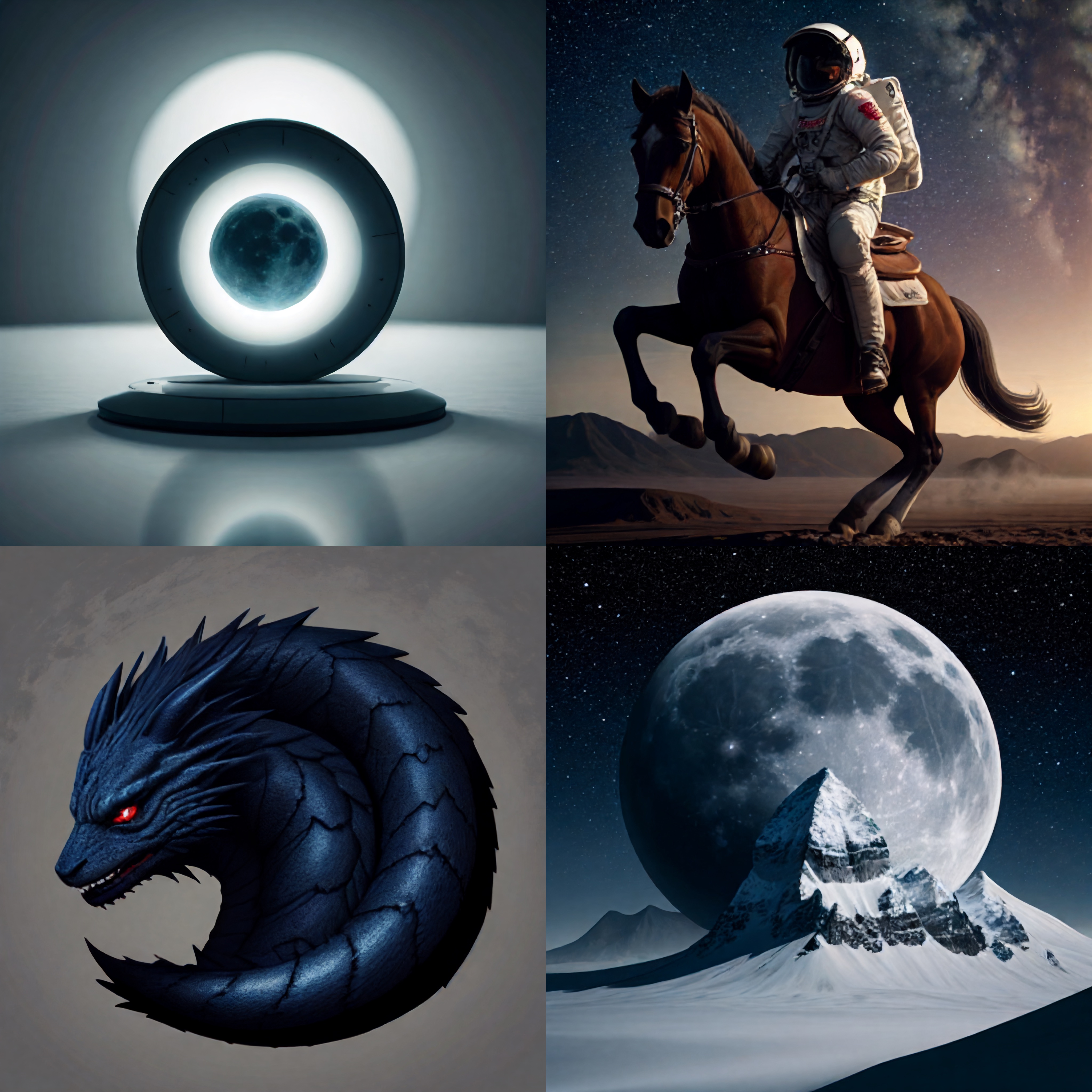
Figure 17: Samples from the Coupling Flow Matching model on top of LCM-LoRA in 2k resolution. Samples are generated in latent space $64^{2}$ and up-sampled with CFM from $64^{2}$ to $256^{2}$. The resulting image has a resolution of $2048\times 2048$. Best viewed when zoomed-in.

GT	REG	LR	FM

Figure 18: Qualitative comparison of the Flow Matching (FM) model to the upsampled low resolution image (LR) the regression model (REG) and the ground truth (GT) using zoomed-in patches. The FM patches are significantly sharper and display more fine-grained details.

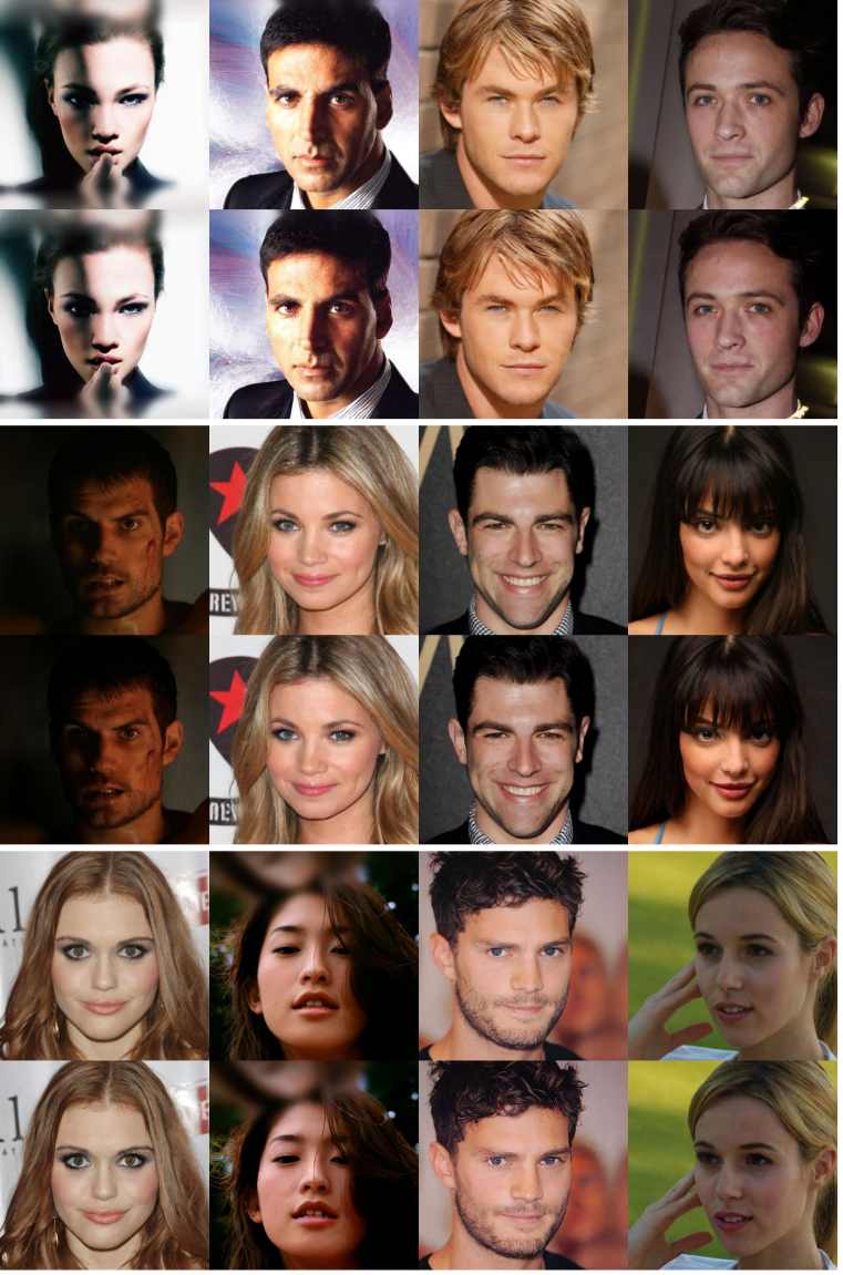
Figure 19: Uncurated samples from the Coupling Flow Matching model on FacesHQ. Up-sampling in latent space from $32\times 32$ to $128\times 128$. Resulting image with resolution of $1024\times 1024$ (bottom) compared to the low-resolution image, up-sampled to $1024\times 1024$ (top). Best viewed when zoomed-in.

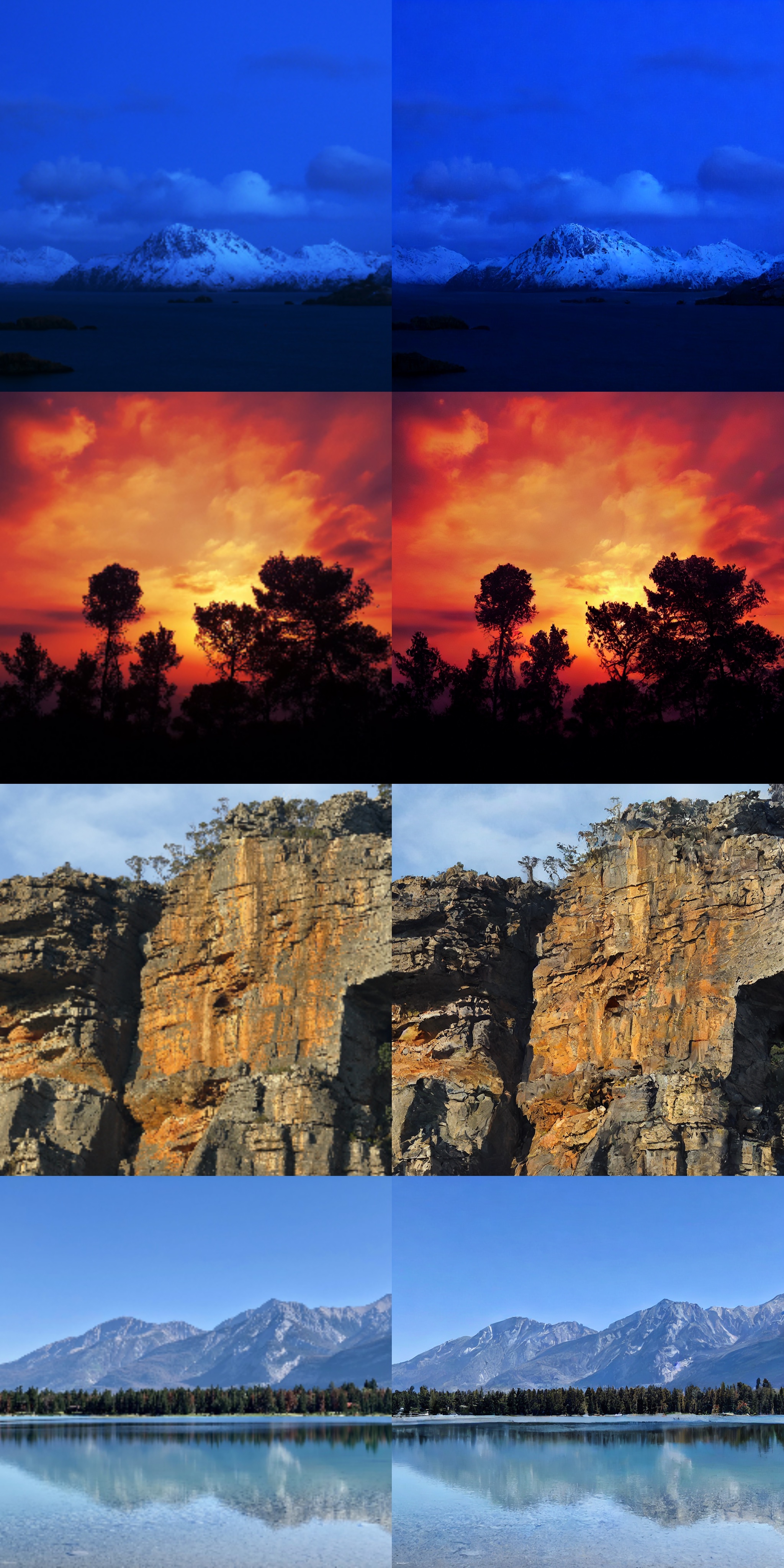
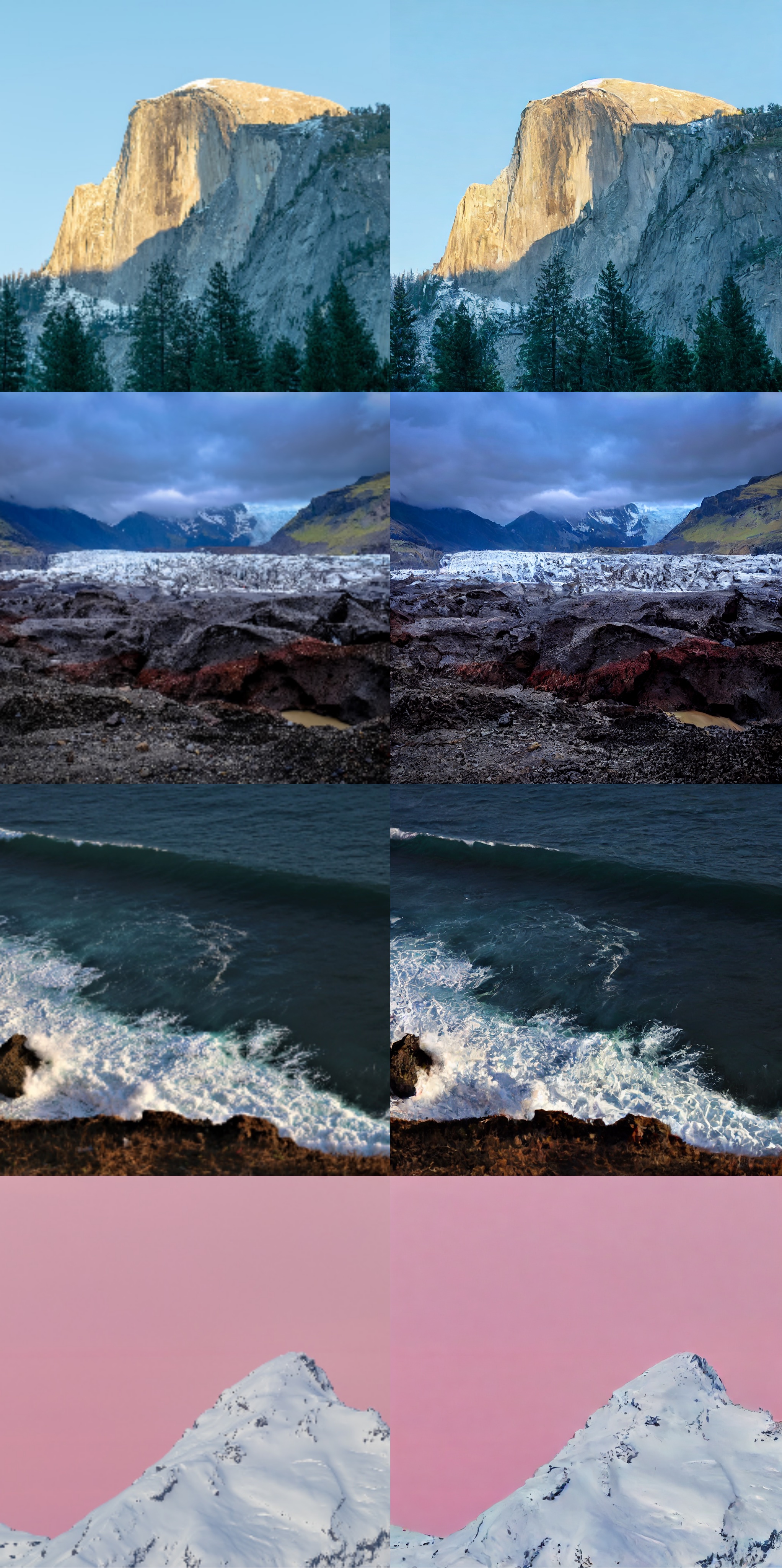
Figure 20: LHQ super-resolution samples. Left: low-resolution ground truth image bi-linearly up-sampled. Right: synthesized high resolution image. Best viewed when zoomed in.

References

- [1] LAION-Aesthetics | https://laion.ai/blog/laion-aesthetics.
- [2] OpenAI | https://github.com/openai/guided-diffusion/blob/main/guided_diffusion/unet.py.
- [3] Unsplash | https://unsplash.com/data.
- Albergo and Vanden-Eijnden [2023] Michael S Albergo and Eric Vanden-Eijnden. Building normalizing flows with stochastic interpolants. In ICLR, 2023.
- Albergo et al. [2023] Michael S Albergo, Mark Goldstein, Nicholas M Boffi, Rajesh Ranganath, and Eric Vanden-Eijnden. Stochastic interpolants with data-dependent couplings. arXiv preprint arXiv:2310.03725, 2023.
- Aram Davtyan and Favaro [2023] Sepehr Sameni Aram Davtyan and Paolo Favaro. Efficient video prediction via sparsely conditioned flow matching. In ICCV, 2023.
- Balaji et al. [2022] Yogesh Balaji, Seungjun Nah, Xun Huang, Arash Vahdat, Jiaming Song, Karsten Kreis, Miika Aittala, Timo Aila, Samuli Laine, Bryan Catanzaro, et al. ediffi: Text-to-image diffusion models with an ensemble of expert denoisers. arXiv preprint arXiv:2211.01324, 2022.
- Blattmann et al. [2023] Andreas Blattmann, Robin Rombach, Huan Ling, Tim Dockhorn, Seung Wook Kim, Sanja Fidler, and Karsten Kreis. Align your latents: High-resolution video synthesis with latent diffusion models. In CVPR, 2023.
- Caron et al. [2021] Mathilde Caron, Hugo Touvron, Ishan Misra, Hervé Jégou, Julien Mairal, Piotr Bojanowski, and Armand Joulin. Emerging properties in self-supervised vision transformers. In Proceedings of the IEEE/CVF international conference on computer vision, pages 9650–9660, 2021.
- Chen et al. [2023] Junsong Chen, Jincheng Yu, Chongjian Ge, Lewei Yao, Enze Xie, Yue Wu, Zhongdao Wang, James Kwok, Ping Luo, Huchuan Lu, et al. Fast training of diffusion transformer for photorealistic text-to-image synthesis. arXiv preprint arXiv:2310.00426, 2023.
- Chen [2018] Ricky T. Q. Chen. torchdiffeq, 2018.
- Dao et al. [2023] Quan Dao, Hao Phung, Binh Nguyen, and Anh Tran. Flow matching in latent space. arXiv preprint arXiv:2307.08698, 2023.
- Esser et al. [2021] Patrick Esser, Robin Rombach, and Bjorn Ommer. Taming transformers for high-resolution image synthesis. In Proceedings of the IEEE/CVF conference on computer vision and pattern recognition, pages 12873–12883, 2021.
- Esser et al. [2023] Patrick Esser, Johnathan Chiu, Parmida Atighehchian, Jonathan Granskog, and Anastasis Germanidis. Structure and content-guided video synthesis with diffusion models. In Proceedings of the IEEE/CVF International Conference on Computer Vision, pages 7346–7356, 2023.
- Goodfellow et al. [2020] Ian Goodfellow, Jean Pouget-Abadie, Mehdi Mirza, Bing Xu, David Warde-Farley, Sherjil Ozair, Aaron Courville, and Yoshua Bengio. Generative adversarial networks. Communications of the ACM, 63(11):139–144, 2020.
- Heusel et al. [2017] Martin Heusel, Hubert Ramsauer, Thomas Unterthiner, Bernhard Nessler, and Sepp Hochreiter. Gans trained by a two time-scale update rule converge to a local nash equilibrium. Advances in neural information processing systems, 30, 2017.
- Ho and Salimans [2022] Jonathan Ho and Tim Salimans. Classifier-free diffusion guidance. arXiv preprint arXiv:2207.12598, 2022.
- Ho et al. [2020] Jonathan Ho, Ajay Jain, and Pieter Abbeel. Denoising diffusion probabilistic models. In NeurIPS, 2020.
- Ho et al. [2022a] Jonathan Ho, Chitwan Saharia, William Chan, David J Fleet, Mohammad Norouzi, and Tim Salimans. Cascaded diffusion models for high fidelity image generation. The Journal of Machine Learning Research, 23(1):2249–2281, 2022a.
- Ho et al. [2022b] Jonathan Ho, Tim Salimans, Alexey Gritsenko, William Chan, Mohammad Norouzi, and David J Fleet. Video diffusion models. In arXiv, 2022b.
- Hu et al. [2024] Tao Hu, David W Zhang, Pascal Mettes, Meng Tang, Deli Zhao, and Cees G.M. Snoek. Latent space editing in transformer-based flow matching. In AAAI, 2024.
- Jin et al. [2023] Zhiyu Jin, Xuli Shen, Bin Li, and Xiangyang Xue. Training-free Diffusion Model Adaptation for Variable-Sized Text-to-Image Synthesis, 2023. arXiv:2306.08645 [cs, eess].
- Kang et al. [2023] Minguk Kang, Jun-Yan Zhu, Richard Zhang, Jaesik Park, Eli Shechtman, Sylvain Paris, and Taesung Park. Scaling up gans for text-to-image synthesis. In Proceedings of the IEEE/CVF Conference on Computer Vision and Pattern Recognition, pages 10124–10134, 2023.
- Karras et al. [2017] Tero Karras, Timo Aila, Samuli Laine, and Jaakko Lehtinen. Progressive growing of gans for improved quality, stability, and variation. arXiv preprint arXiv:1710.10196, 2017.
- Karras et al. [2019] Tero Karras, Samuli Laine, and Timo Aila. A style-based generator architecture for generative adversarial networks. In CVPR, 2019.
- Karras et al. [2022] Tero Karras, Miika Aittala, Timo Aila, and Samuli Laine. Elucidating the design space of diffusion-based generative models. In NeurIPS, 2022.
- Kingma et al. [2021] Diederik Kingma, Tim Salimans, Ben Poole, and Jonathan Ho. Variational diffusion models. In NeurIPS, 2021.
- Le et al. [2023] Matthew Le, Apoorv Vyas, Bowen Shi, Brian Karrer, Leda Sari, Rashel Moritz, Mary Williamson, Vimal Manohar, Yossi Adi, Jay Mahadeokar, et al. Voicebox: Text-guided multilingual universal speech generation at scale. In arXiv, 2023.
- Ledig et al. [2017] Christian Ledig, Lucas Theis, Ferenc Huszár, Jose Caballero, Andrew Cunningham, Alejandro Acosta, Andrew Aitken, Alykhan Tejani, Johannes Totz, Zehan Wang, et al. Photo-realistic single image super-resolution using a generative adversarial network. In Proceedings of the IEEE conference on computer vision and pattern recognition, pages 4681–4690, 2017.
- Li et al. [2022] Haoying Li, Yifan Yang, Meng Chang, Shiqi Chen, Huajun Feng, Zhihai Xu, Qi Li, and Yueting Chen. Srdiff: Single image super-resolution with diffusion probabilistic models. Neurocomputing, 479:47–59, 2022.
- Li et al. [2023] Yuheng Li, Haotian Liu, Qingyang Wu, Fangzhou Mu, Jianwei Yang, Jianfeng Gao, Chunyuan Li, and Yong Jae Lee. Gligen: Open-set grounded text-to-image generation. In Proceedings of the IEEE/CVF Conference on Computer Vision and Pattern Recognition, pages 22511–22521, 2023.
- Lipman et al. [2023] Yaron Lipman, Ricky T. Q. Chen, Heli Ben-Hamu, Maximilian Nickel, and Matthew Le. Flow matching for generative modeling. In ICLR, 2023.
- Liu et al. [2023a] Haohe Liu, Zehua Chen, Yi Yuan, Xinhao Mei, Xubo Liu, Danilo Mandic, Wenwu Wang, and Mark D Plumbley. Audioldm: Text-to-audio generation with latent diffusion models. In ICML, 2023a.
- Liu et al. [2022] Luping Liu, Yi Ren, Zhijie Lin, and Zhou Zhao. Pseudo numerical methods for diffusion models on manifolds. In ICLR, 2022.
- Liu et al. [2023b] Xingchao Liu, Chengyue Gong, and Qiang Liu. Flow straight and fast: Learning to generate and transfer data with rectified flow. In ICLR, 2023b.
- Lu et al. [2022a] Cheng Lu, Yuhao Zhou, Fan Bao, Jianfei Chen, Chongxuan Li, and Jun Zhu. Dpm-solver: A fast ode solver for diffusion probabilistic model sampling in around 10 steps. NeurIPS, 2022a.
- Lu et al. [2022b] Cheng Lu, Yuhao Zhou, Fan Bao, Jianfei Chen, Chongxuan Li, and Jun Zhu. Dpm-solver++: Fast solver for guided sampling of diffusion probabilistic models. arXiv preprint arXiv:2211.01095, 2022b.
- Luo et al. [2023a] Simian Luo, Yiqin Tan, Longbo Huang, Jian Li, and Hang Zhao. Latent consistency models: Synthesizing high-resolution images with few-step inference. arXiv preprint arXiv:2310.04378, 2023a.
- Luo et al. [2023b] Simian Luo, Yiqin Tan, Suraj Patil, Daniel Gu, Patrick von Platen, Apolinário Passos, Longbo Huang, Jian Li, and Hang Zhao. Lcm-lora: A universal stable-diffusion acceleration module. arXiv preprint arXiv:2311.05556, 2023b.
- Meng et al. [2023] Chenlin Meng, Robin Rombach, Ruiqi Gao, Diederik Kingma, Stefano Ermon, Jonathan Ho, and Tim Salimans. On distillation of guided diffusion models. In Proceedings of the IEEE/CVF Conference on Computer Vision and Pattern Recognition, pages 14297–14306, 2023.
- Neklyudov et al. [2023] Kirill Neklyudov, Rob Brekelmans, Daniel Severo, and Alireza Makhzani. Action matching: Learning stochastic dynamics from samples. In ICML, 2023.
- Nichol et al. [2021] Alex Nichol, Prafulla Dhariwal, Aditya Ramesh, Pranav Shyam, Pamela Mishkin, Bob McGrew, Ilya Sutskever, and Mark Chen. Glide: Towards photorealistic image generation and editing with text-guided diffusion models. arXiv preprint arXiv:2112.10741, 2021.
- Nichol and Dhariwal [2021] Alexander Quinn Nichol and Prafulla Dhariwal. Improved denoising diffusion probabilistic models. In ICML, 2021.
- Podell et al. [2023] Dustin Podell, Zion English, Kyle Lacey, Andreas Blattmann, Tim Dockhorn, Jonas Müller, Joe Penna, and Robin Rombach. Sdxl: Improving latent diffusion models for high-resolution image synthesis. arXiv preprint arXiv:2307.01952, 2023.
- Preechakul et al. [2022] Konpat Preechakul, Nattanat Chatthee, Suttisak Wizadwongsa, and Supasorn Suwajanakorn. Diffusion autoencoders: Toward a meaningful and decodable representation. In CVPR, 2022.
- Rabe and Staats [2021] Markus N Rabe and Charles Staats. Self-attention does not need memory. arXiv preprint arXiv:2112.05682, 2021.
- Ramesh et al. [2022] Aditya Ramesh, Prafulla Dhariwal, Alex Nichol, Casey Chu, and Mark Chen. Hierarchical text-conditional image generation with clip latents. arXiv preprint arXiv:2204.06125, 1(2):3, 2022.
- Rombach et al. [2022] Robin Rombach, Andreas Blattmann, Dominik Lorenz, Patrick Esser, and Björn Ommer. High-resolution image synthesis with latent diffusion models. In CVPR, 2022.
- Ronneberger et al. [2015] Olaf Ronneberger, Philipp Fischer, and Thomas Brox. U-net: Convolutional networks for biomedical image segmentation. In Medical Image Computing and Computer-Assisted Intervention–MICCAI 2015: 18th International Conference, Munich, Germany, October 5-9, 2015, Proceedings, Part III 18, pages 234–241. Springer, 2015.
- Saharia et al. [2022a] Chitwan Saharia, William Chan, Saurabh Saxena, Lala Li, Jay Whang, Emily L Denton, Kamyar Ghasemipour, Raphael Gontijo Lopes, Burcu Karagol Ayan, Tim Salimans, et al. Photorealistic text-to-image diffusion models with deep language understanding. Advances in Neural Information Processing Systems, 35:36479–36494, 2022a.
- Saharia et al. [2022b] Chitwan Saharia, Jonathan Ho, William Chan, Tim Salimans, David J Fleet, and Mohammad Norouzi. Image super-resolution via iterative refinement. TPAMI, 45(4):4713–4726, 2022b.
- Salimans and Ho [2022] Tim Salimans and Jonathan Ho. Progressive distillation for fast sampling of diffusion models. In ICLR, 2022.
- Schuhmann et al. [2022] Christoph Schuhmann, Romain Beaumont, Richard Vencu, Cade Gordon, Ross Wightman, Mehdi Cherti, Theo Coombes, Aarush Katta, Clayton Mullis, Mitchell Wortsman, et al. Laion-5b: An open large-scale dataset for training next generation image-text models. Advances in Neural Information Processing Systems, 35:25278–25294, 2022.
- Singer et al. [2022] Uriel Singer, Adam Polyak, Thomas Hayes, Xi Yin, Jie An, Songyang Zhang, Qiyuan Hu, Harry Yang, Oron Ashual, Oran Gafni, et al. Make-a-video: Text-to-video generation without text-video data. arXiv preprint arXiv:2209.14792, 2022.
- Skorokhodov et al. [2021] Ivan Skorokhodov, Grigorii Sotnikov, and Mohamed Elhoseiny. Aligning latent and image spaces to connect the unconnectable. In Proceedings of the IEEE/CVF International Conference on Computer Vision, pages 14144–14153, 2021.
- Sohl-Dickstein et al. [2015] Jascha Sohl-Dickstein, Eric Weiss, Niru Maheswaranathan, and Surya Ganguli. Deep unsupervised learning using nonequilibrium thermodynamics. In ICML, 2015.
- Song et al. [2021a] Jiaming Song, Chenlin Meng, and Stefano Ermon. Denoising diffusion implicit models. In ICLR, 2021a.
- Song et al. [2021b] Yang Song, Jascha Sohl-Dickstein, Diederik P Kingma, Abhishek Kumar, Stefano Ermon, and Ben Poole. Score-based generative modeling through stochastic differential equations. In ICLR, 2021b.
- Song et al. [2023] Yang Song, Prafulla Dhariwal, Mark Chen, and Ilya Sutskever. Consistency models. In ICML, 2023.
- Tong et al. [2023] Alexander Tong, Nikolay Malkin, Guillaume Huguet, Yanlei Zhang, Jarrid Rector-Brooks, Kilian Fatras, Guy Wolf, and Yoshua Bengio. Improving and generalizing flow-based generative models with minibatch optimal transport. In ICML, 2023.
- Wang et al. [2018] Xintao Wang, Ke Yu, Shixiang Wu, Jinjin Gu, Yihao Liu, Chao Dong, Yu Qiao, and Chen Change Loy. Esrgan: Enhanced super-resolution generative adversarial networks. In Proceedings of the European conference on computer vision (ECCV) workshops, pages 0–0, 2018.
- Xiao et al. [2021] Zhisheng Xiao, Karsten Kreis, and Arash Vahdat. Tackling the generative learning trilemma with denoising diffusion gans. arXiv preprint arXiv:2112.07804, 2021.
- Xue et al. [2023] Zeyue Xue, Guanglu Song, Qiushan Guo, Boxiao Liu, Zhuofan Zong, Yu Liu, and Ping Luo. Raphael: Text-to-image generation via large mixture of diffusion paths. arXiv preprint arXiv:2305.18295, 2023.
- Yue et al. [2023] Zongsheng Yue, Jianyi Wang, and Chen Change Loy. Resshift: Efficient diffusion model for image super-resolution by residual shifting. arXiv preprint arXiv:2307.12348, 2023.
- Zhang et al. [2021] Kai Zhang, Jingyun Liang, Luc Van Gool, and Radu Timofte. Designing a practical degradation model for deep blind image super-resolution. In Proceedings of the IEEE/CVF International Conference on Computer Vision, pages 4791–4800, 2021.
- Zhang et al. [2023] Lvmin Zhang, Anyi Rao, and Maneesh Agrawala. Adding conditional control to text-to-image diffusion models. In Proceedings of the IEEE/CVF International Conference on Computer Vision, pages 3836–3847, 2023.