Impact of Array Configuration on Head-Mounted Display Performance at mmWave Bands

Abstract

Immersing a user in life-like extended reality (XR) scenery using a head-mounted display (HMD) with a constrained form factor and hardware complexity requires remote rendering on a nearby edge server or computer. Millimeter-wave (mmWave) communication technology can provide sufficient data rate for wireless XR content transmission. However, mmWave channels exhibit severe sparsity in the angular domain. This means that distributed antenna arrays are required to cover a larger angular area and to combat outage during HMD rotation. At the same time, one would prefer fewer antenna elements/arrays for a lower complexity system. Therefore, it is important to evaluate the trade-off between the number of antenna arrays and the achievable performance to find a proper practical solution. This work presents indoor 28 GHz mmWave channel measurement data, collected during HMD mobility, and studies the dominant eigenmode (DE) gain. DE gain is a significant factor in understanding system performance since mmWave channel sparsity and eigenmode imbalance often results in provisioning the majority of the available power to the DE. Moreover, it provides the upper performance bounds for widely-adopted analog beamformers. We propose 3 performance metrics – gain trade-off, gain volatility, and minimum service trade-off – for evaluating the performance of a multi-array HMD and apply the metrics to indoor 28 GHz channel measurement data. Evaluation results indicate, that 3 arrays provide stable temporal channel gain. Adding a 4^th array further increases channel capacity, while any additional arrays do not significantly increase physical layer performance.

I Introduction

An extended reality (XR) head-mounted display (HMD) aims to immerse the user in a virtual environment or intertwine digital objects with the user’s physical surroundings. An HMD primarily focuses on deceiving the human visual system by means of high-resolution video data, requiring powerful graphics processing unit (GPU) rendering hardware. To avoid burdening the HMD with additional processing components and batteries, rendering can take place at either an edge server [1] or a nearby computer, requiring transport medium data rates in excess of $1\text{\,}\mathrm{G}\mathrm{b}\mathrm{p}\mathrm{s}$ and more than $10\text{\,}\mathrm{G}\mathrm{b}\mathrm{p}\mathrm{s}$ for streaming unencoded video. HMDs, therefore, often rely on a tethered connection to the rendering machine. However, a cable will hinder user mobility and compromise XR content fidelity – the reason for needing to transfer video data in the first place. Wireless communication technologies 5G, 6G, and IEEE 802.11ad/ay can supply peak multi-Gbps data rates by leveraging the ample bandwidth availability in the millimeter-wave (mmWave) and THz spectrum [2, 3, 4]. Unfortunately, mmWave channels are known for their angular sparsity, i.e., having few distinct multipath components (MPCs) [5, 6]. Hence, an HMD, equipped with widely-adopted directional patch antennas (with a field of view less than $<90^{\circ}$ [7]) should feature several antenna arrays, placed along the HMD’s outside perimeter, to provide sufficient angular coverage during rotation. In addition to misalignment, mmWave MPCs are highly prone to blockage by other users and oneself [8, 9]. Adding antenna arrays can also mitigate the adverse effects of blockage since the broader angular coverage allows the HMD to receive other MPCs (reflections, unaffected by blockage).

MmWave reception quality has recently been studied in the context of 5G NR mobile networks. Handheld devices are subject to usage in adverse circumstances – movement, orientation flipping, shadowing, and physical contact between its antennas and the user – that can disturb the mmWave data link. Walking $15\text{\,}\mathrm{m}$ from one end of a corridor to its far end will cause a degradation of around $1520\text{\,}\mathrm{dB}$, with additional $\pm$$15\text{\,}\mathrm{dB}$ fluctuations depending on the specific user [10]. Rotating the smartphone from vertical to horizontal orientation can further cause a two-fold change in the achieved performance, e.g., [11] notes a decrease in IEEE 802.11ad data rate by half upon orientation change. User body shadowing can effectively attenuate $2025\text{\,}\mathrm{dB}$ in various handheld use cases [12]. A palm, holding the smartphone, will absorb up to $15\text{\,}\mathrm{dB}$ signal strength, whereas a mere finger interacting with the handheld device can already disturb the mmWave data link gain by $3\text{\,}\mathrm{dB}$ [13]. All these issues can plague XR HMDs mmWave communications systems. Previous studies concerning mmWave channel measurements for XR HMDs have demonstrated, that high data rates are achievable in cluttered indoor scenarios even with limited mmWave link bandwidth [14], and that a device featuring a single phase-shifted mmWave array will result in inappropriately volatile channel conditions for XR video content streaming [15]. However, horn antennas and first-generation consumer off-the-shelf (COTS) equipment, used in prior art, offer limited insight into how future HMDs, employing mmWave technology might perform. In the work at hand, we utilize a multi-antenna-array mmWave channel sounder to assess channel conditions during small-scale HMD movement due to head rotation, as well as large-scale fading due to line of sight (LoS) obstruction. We pursue the answers to: 1) What are the important physical layer performance metrics for configuring multiple mmWave antenna arrays on an HMD? 2) What is the minimal number of antenna arrays that still allows the HMD to reap the benefits of high-bandwidth mmWave communications? Performance is evaluated based on the channel’s dominant eigenmode (DE) gain. The reason for this is, that mmWave channels are sparse, and any additional eigenmodes, beyond the first, are of much lower quality. Hence, often the best strategy for applications with high data rate and somewhat looser reliability requirements, compared to vehicular and industrial applications, is allocating most if not all power to the dominant eigenmode. Leveraging on a dedicated measurement campaign, our contributions are:

• MmWave channel DE transmission performance is evaluated for a multi-array HMD during rotation.

• Physical layer performance metrics, relevant for antenna array configuration on an HMD, are proposed.

• The profitability of using a rear headband on the HMD as an antenna array mounting point is assessed.

Section II describes the experiment setup. The post-processing procedures and proposed performance metrics are introduced in Section III and used in Section IV to evaluate $28\text{\,}\mathrm{GHz}$ channel measurements. Lastly, Section V summarizes the work and outlines future research directions.

II Experiment setup

II-A Measurement equipment

We collect channel impulse response (CIR) data using a switched array multiple-input multiple-output (MIMO) channel sounder [16], custom-built by Lund University and SONY. The sounder operates at $28\text{\,}\mathrm{GHz}$ with a $768\text{\,}\mathrm{MHz}$ bandwidth ($1.3\text{\,}\mathrm{ns}$ time-delay resolution) and employs a Zadoff-Chu waveform. A top-down view of the user equipment (UE) is illustrated in Fig. 1. It consists of 8 planar patch antenna arrays, referred to as panels, offset by $45\text{\,}\mathrm{\SIUnitSymbolDegree}$ in azimuth and featuring $4\text{\,}$$\times$$4\text{\,}$ antennas each. Fig. 1 shows the studied forward-facing 1–7 panel configurations using the outer octagons. These are used throughout the work at hand, since we envision that future XR HMDs will prioritize both ergonomics and aesthetics; hence, they will not feature a rear headband by default. The inner octagons show the backward-facing configurations, evaluated only in Section IV-D. Conversely, the access point (AP) features a single $16\text{\,}$$\times$$4\text{\,}$ planar array. All antenna elements are dual-polarized, resulting in a $256\text{\,}$$\times$$128\text{\,}$ channel matrix. Sampling is done at $18.3\text{\,}\mathrm{\SIUnitSymbolMicro s}$ per antenna element combination, which includes averaging over 4 sounding sequences to reduce measurement noise. The CIR snapshot sampling rate is $1\text{\,}\mathrm{Hz}$ to allow additional time for memory writing. Rubidium clocks and additional preambles in the sounding waveform are used for accurate synchronization. Table I summarizes the system parameters, while we refer the reader to [tataria_275-295_2021] for further details on the channel sounder. Fig. 2(b) includes a picture of the UE and AP. Note, that although we consider relatively large UE antenna arrays (approx. $2.5\text{\,}$$\times$$2.5\text{\,}\mathrm{cm}$), the learnings presented in this work are also applicable to smaller arrays with less elements since we study the trade-offs between a full 8-panel setup and an HMD with less antenna panels.

TABLE I: System parameters.

Parameter	Value
Carrier frequency	$28\text{\,}\mathrm{GHz}$
Bandwidth	$768\text{\,}\mathrm{MHz}$
Time-delay resolution	$1.3\text{\,}\mathrm{ns}$
Max. observable time-delay	$2.7\text{\,}\mathrm{\SIUnitSymbolMicro s}$
Element combination sampling time	$18.3\text{\,}\mathrm{\SIUnitSymbolMicro s}$
CIR snapshot sampling frequency	$1\text{\,}\mathrm{Hz}$
Single-position measurement duration	$33\text{\,}\mathrm{s}$
AP array size	4$\times$16
UE array size	4$\times$4
Number of UE arrays (panels)	8
CIR snapshot size	$256\times 128\times 2048$

Figure 1: UE top-down view, showing the forward- and backward-facing 1–7 panel configurations on the HMD.

II-B Measurement environment

Measurements were carried out at 11 discrete random positions in a conference room, depicted in Fig. 2. The initial UE orientation is randomly selected for each position and is shown by the red line at each UE position in Fig. 2(a). This orientation serves as the starting point for the mobility pattern, described in Section II-C. Channel sounding is repeated at each position for non-line-of-sight (NLoS) conditions, where a fiberglass water-filled human phantom [8] represents a person obstructing the LoS. Since the phantom was initially designed for $60\text{\,}\mathrm{GHz}$ experiments, we first characterized it against 6 volunteers at $28\text{\,}\mathrm{GHz}$. The difference in attenuation between the phantom and the human subjects ranges from $-0.6\text{\,}$ to $2.1\text{\,}\mathrm{dB}$, hence, the phantom is suited for $28\text{\,}\mathrm{GHz}$ experiments. The environment remains static during CIR sampling, except for UE mobility, detailed in the upcoming subsection.

(a) Floor plan. Brown, cyan, gray, and magenta mark tables and the door, windows, metal whiteboards, and a projector screen, respectively. The room size is $6\times$$9.15\text{\,}\mathrm{m}$.

(b) Setup for UE₆, NLoS. Superimposed: mean difference between the phantom’s attenuation and that of 6 human subjects (in $\text{\,}\mathrm{dB}$).

Figure 2: Conference room measurement environment.

II-C Mobility pattern

A UE mobility pattern, outlined in Fig. 3, has been designed to mimic different possible HMD rotations during usage. Initially, the UE is standing upright with panel VII oriented in the direction shown in Fig. 2(a). Recall from Fig. 1 that panel VII is oriented in the HMD looking direction. A $\Delta\alpha=30^{\circ}$ leftward (positive) yaw rotation is executed first, followed by pitching $\Delta\beta=30^{\circ}$ towards the ground, and concluded by a second $\Delta\alpha=30^{\circ}$ leftward rotation in yaw, while pitched downwards. All rotations are of extrinsic $xyz$ Euler type. Movement is executed by manually rotating the tripod’s head, on which the UE is mounted. Antenna velocity is kept below $1\text{\,}\mathrm{cm}\text{\,}{\mathrm{s}}^{-1}$, thus, less than one carrier wavelength per second. Considering the $25\text{\,}\mathrm{cm}$ distance (marked on the left side of Fig. 3) between the center of rotation and the octagonal UE’s center of mass – representing the offset between an HMD and the human cervical vertebrae [17] – the $30$-$30$-$30^{\circ}$ pattern requires $3$-$15$-$15$ $\text{\,}\mathrm{s}$ or $33\text{\,}\mathrm{s}$ in total. We refer to the resulting 33 CIR matrices as one measurement. Note, that the second and third rotation displaces the UE’s center of mass by approximately $13\text{\,}$ and $6.5\text{\,}\mathrm{cm}$, correspondingly, which make it lean beyond the phantom during parts of NLoS measurements.

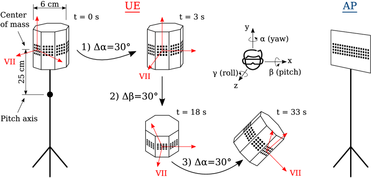
Figure 3: UE mobility pattern in extrinsic Euler rotations.

III Post-processing procedures

In this work, we evaluate the DE gain, i.e., the gain of single-spatial-stream transmission with channel information at both AP and UE, per orthogonal frequency-division multiplexing (OFDM) subcarrier, for different UE antenna panel configurations. As previously mentioned, the combination of high data rate and loose reliability requirements, combined with channel sparsity, in practice results in the majority of power being allocated to the DE. For example, when applying waterfilling [18]. Furthermore, when evaluated over the entire bandwidth, the DE transmission scheme’s gain provides both the upper gain bound for analog beamformers, often found in mmWave COTS devices, and the average gain of a joint spectral-spatial OFDM -MIMO precoder, commonly found in lower-frequency cellular and IEEE 802.11 networks. Note that fully-digital MIMO and hybrid beamforming can in practice reach higher channel capacity in the absence of a dominant signal component, while the latter also manages to maintain relatively high energy efficiency [19]. Both fully-digital MIMO and hybrid beamforming are beyond the scope of this work. For clarity, Table II lists the relevant indices in this section.

TABLE II: Index overview.

Index	Meaning	Index	Meaning
p	Number of UE panels	i	Channel snapshot index
u	UE position	k	Subcarrier index
s	LoS/NLoS scenario

III-A De-noising and dominant eigenvalue extraction

We first de-noise the CIR to minimize the amount of noise that propagates into the frequency domain upon Fourier transformation (sum over CIR samples), enabling us to observe lower DE gain, e.g., for a single array configuration in NLoS conditions, without it sinking below the noise floor. Let $\bm{H}(\tau)$ denote the 2-dimensional MIMO CIR at delay $\tau$ and let $\lambda_{1}(\tau)\geq...\geq\lambda_{n}(\tau)$ be the squared singular values of $\bm{H}(\tau)$ (eigenvalues of $\bm{H}\bm{H}^{H}$). We apply the de-noising procedure outlined in Algorithm 1. First, we select $\lambda_{1}(\tau)$ values at time delays far exceeding any reasonable or observed MPC delays, i.e., $\tau\in(1.35,2.7)$ $\text{\,}\mathrm{\SIUnitSymbolMicro s}$ (second half of the CIR). The result is a vector of the largest eigenvalues of 1024 noisy square matrices, denoted as $\bm{\lambda}_{\text{noise}}$. The values have a Tracy-Widom $\mathcal{T}\mathcal{W}_{2}$ distribution [20], and, due to the limited CIR dimensions, we use the 95^th percentile as the noise threshold, instead of applying, for example, the Marčenko-Pastur law. Next, we apply the eigenvalue threshold $\Lambda$ for setting noisy CIR samples to 0. Finally, all CIR entries exceeding the $\tau_{\text{max}}=105$ $\text{\,}\mathrm{ns}$ delay spread, corresponding to $31.5\text{\,}\mathrm{m}$ or the longest path traveled by a 2^nd order reflection, are suppressed to 0. This leaves us with at most 80 non-zero CIR samples. We estimate the potential gain loss by considering the worst-case scenario, where 64 of the 80 windowed samples ($105\text{\,}\mathrm{ns}$) represent at least 2^nd order reflections with a gain just below the threshold $\Lambda$, and that $18\text{\,}\mathrm{dB}$ separates the gain of the LoS and the reflected MPCs– $8\text{\,}\mathrm{dB}$ for path loss and $2\text{\,}$$\times$$5\text{\,}\mathrm{dB}$ for reflections. Then the calculated DE gain after de-noising would be $3\text{\,}\mathrm{dB}$ too low. Contrarily, removing 64/80 noisy CIR samples from the summation in the Fourier transform allows us to study $18\text{\,}\mathrm{dB}$ smaller eigenmodes in the frequency domain.

Algorithm 1 CIR de-noising

1:procedure De-noise($\bm{H}$)

2:  $\bm{\lambda}_{\text{noise}}=\lambda_{1}(\tau),\text{ for }\tau\in(1.35,2.7)$ $\text{\,}\mathrm{\SIUnitSymbolMicro s}$ $\triangleright$ Evaluate noise

3:  $\Lambda=P_{95}(\bm{\lambda}_{\text{noise}})$ $\triangleright$ Get threshold

4:  $\bm{H}(\tau)\leftarrow\bm{0},\text{ where }\bm{\lambda}_{\text{noise}}<\Lambda$ $\triangleright$ Below threshold

5:  $\bm{H}(\tau)\leftarrow\bm{0},\text{ for }\tau>\tau_{\text{max}}$ $\triangleright$ Out of delay spread

6:end procedure

We convert each CIR to its channel transfer function (CTF) using the fast Fourier transform (FFT), before extracting the dominant eigenmode gain per subcarrier. We use a 2048-point FFT for convenience since the CIR has 2048 time-delay samples. All further mention of eigenvalues/modes refers explicitly to the frequency domain. We drop the index ₁ in view of brevity and denote the $k$-th tone’s dominant eigenmode as $\lambda[u,s,i,k]$, where $k\in[0,2047]$ ($27.61628.384\text{\,}\mathrm{GHz}$), while $u$, $s$, and $i$ represent the UE position, scenario (LoS/NLoS), and channel snapshot index, correspondingly (see Table II).

III-B Performance metrics

This section proposes processing procedures for evaluating the performance of a 1–7 panel HMD, based on $\lambda[u,s,i,k]$, where $u,s,i,k$ are listed in Table II.

III-B1 Gain trade-off

The first metric is the DE gain trade-off between a full 8-panel HMD and a p-panel HMD. It allows us to identify whether changing the panel count results in merely a gain difference proportional to beamforming gain or if there are other driving forces behind the difference, such as diversity gain. The trade-off is derived as follows:

$$\overline{\Delta\lambda_{p}}[u,s,i]=\frac{1}{K}\sum_{k=0}^{K-1}\frac{\lambda_{p}[u,s,i,k]}{\lambda_{8}[u,s,i,k]},$$ (1)

where $\lambda_{p}[u,s,i,k]$ and $\lambda_{8}[u,s,i,k]$ are the DEs of a p-panel and an 8-panel HMD. An average over 2048 subcarriers for each channel snapshot constitutes the final value.

III-B2 Gain volatility

An important performance metric for XR applications is wireless link stability, since it determines how much video stream buffer is required, how often the resolution is adapted, and whether there is a need for radio access technology switching. Channel gain spread and persistence are evaluated through the gain’s standard deviation and autocorrelation, respectively. The latter is derived according to:

$$r_{p}[u,s]=\frac{\sum\limits_{i=0}^{I-2}(\overline{\lambda_{p}}[u,s,i]\!-\!\overline{\overline{\lambda_{p}}}[u,s])(\overline{\lambda_{p}}[u,s,i\!+\!1]\!-\!\overline{\overline{\lambda_{p}}}[u,s])}{\sum\limits_{i=0}^{I-1}(\overline{\lambda_{p}}[u,s,i]-\overline{\overline{\lambda_{p}}}[u,s])^{2}},$$ (2)

where the number of snapshots per measurement is $I=33$, $\overline{\lambda_{p}}[u,s,i]$ is the average DE over all subcarriers, and $\overline{\overline{\lambda_{p}}}[u,s]$ represents its mean value. The evaluation is carried out independently at each measurement position and for LoS/NLoS scenarios. A high standard deviation will indicate a large DE gain spread during the course of one measurement, while a low autocorrelation is the result of frequent changes in gain over time. Observing both high standard deviation and low autocorrelation, in combination with low average gain, would signal a potentially unstable XR service since there are large variations in the already adverse channel conditions.

III-B3 Minimal service and capacity trade-off

We obtain the minimal service trade-off by comparing the 3^rd percentile DE gain for a p-panel configuration against that of an 8-panel HMD. We use the 3^rd percentile based on the $97\text{\,}\mathrm{\char 37\relax}$ link reliability constraint, corresponding to the largest allowed error ratio for satisfactory encoded video quality [21]. The metric shows how much channel capacity is lost due to employing less panels in the most adverse conditions, without considering $3\text{\,}\mathrm{\char 37\relax}$ of the lowest recorded gains. Assuming $\text{\,}\mathrm{S}\mathrm{N}\mathrm{R}$${}_{p}>>1$, the minimal service trade-off is calculated as follows [18]:

$$\Delta C_{p,97}\;\approx\;\left|\log_{2}\left(\frac{P_{3}(\bm{\overline{\lambda_{p}}})}{P_{3}(\bm{\overline{\lambda_{8}}})}\right)\right|,$$ (3)

where $\bm{\overline{\lambda_{p}}}$ represents a vector of the DEs at each position, scenario, and snapshot ($u$, $s$, $i$), averaged over all 2048 subcarriers ($k$). Furthermore, we derive the channel capacity trade-off for each individual measurement, which allows us to evaluate how much capacity is wasted due to employing less than 8 panels. It is calculated according to:

$$\overline{\Delta C_{p}}[u,s,i]\;\approx\;\left|\frac{1}{K}\sum_{k=0}^{K-1}\log_{2}\left(\frac{\lambda_{p}[u,s,i,k]}{\lambda_{8}[u,s,i,k]}\right)\right|,$$ (4)

where $\overline{\Delta C_{p}}$ represents the mean channel capacity trade-off over all 2048 subcarriers.

III-C Profit from a rear headband

Lastly, we evaluate the benefit of fitting a rear headband to the HMD and placing an antenna panel on it by assessing the overall gain difference between the default, forward-facing, panel configuration and its rotated counterpart. The latter always employs the backward-facing panel III, wheres the former excludes it (see Fig. 1). We use a similar approach to Equation 1 and evaluate the rear headband benefits using:

$$\overline{\Delta\lambda_{p}^{rh}}[u,s,i]=\frac{1}{K}\sum_{k=0}^{K-1}\frac{\lambda_{p,\text{back}}[u,s,i,k]}{\lambda_{p,\text{front}}[u,s,i,k]},$$ (5)

where $\lambda_{p,\text{front}}[u,s,i,k]$ and $\lambda_{p,\text{back}}[u,s,i,k]$ represent the forward- and backward-facing p-panel configuration DE gains.

IV Results

IV-A Gain trade-off and impact of mobility

Fig. 4 plots the DE gain trade-off, dependent on the number of antenna panels. The median gain trade-off, across all channel snapshots (full lines), increases logarithmically with the number of employed panels; however, the observed gain only starts conforming with the beamforming gain for an HMD with 5 or more panels. This leads us to two conclusions 1) the beamforming gain for 1–4 panels is overestimated since not all elements on an 8-panel HMD are illuminated, and 2) 4 panels capture the available diversity gain (sufficient azimuth coverage) and adding any additional panels results in merely beamforming gain. We also observe a reduction in the spread of the distributions as the number of employed panels grows, with the most noticeable improvements from 1 to 2 and from 2 to 3 panels, while 4 panels offer a marginal improvement over 3 panels. Finally, a 4-panel HMD follows the gain trend of an 8-panel HMD the most accurately due to its good symmetry (see Fig. 1), i.e., an evenly distributed azimuth gain.

Figure 4: Gain ratio per mobility pattern (dotted) and combined (full line). Median values are depicted in orange.

The dotted distributions in Fig. 4 show that all, except a 2-panel HMD, experience somewhat better performance during the initial $\Delta\alpha=30^{\circ}$ rotation, when the UE is standing upright. This is most visible for a single-panel HMD. We assume the carpeted floor and numerous table and chair legs result in poor MPC reflection, that the forward-pitched UE could receive. A 2-panel HMD exhibits favorable performance in the final part of the mobility. This is due to the NLoS experiments, where the second $\Delta\alpha=30^{\circ}$ rotation, at some point, directly exposes one of the two panels to the LoS that bypasses the phantom.

IV-B Gain volatility

The gain’s standard deviation ($\delta_{p}$) and autocorrelation ($r_{p}$) are depicted in Fig. 5. The LoS and NLoS scenarios are separated by star/cross markers, while marker size shows the average gain for each of the 22 measurements. A single panel yields high gain volatility, since adjacent measurements (less than 1 cm apart) may exhibit a high difference in gain as the panel moves or rotates from LoS to NLoS or vice-versa. Gain spread remains high for a 2-panel HMD, however, gain perturbations are gradual over time (high autocorrelation). This benefits the HMD since resolution adaptations and handovers are less frequent. An HMD with 3 or more panels shows less pronounced gain spread and higher mean gain. The low autocorrelation points originate from more adverse circumstances, where 3 or 4 panels receive the strongest MPC from a large angle, relative to the individual radiation patterns. For example, take a forward-pitched 4-panel HMD at positions UE₄ or UE₉, where the LoS angle of arrival strides around $\pm$$45\text{\,}\mathrm{\SIUnitSymbolDegree}$ or right in-between two panels. Yet, this is a less severe problem since fluctuations around a high mean gain are less likely to cause service outage. Conversely, a 2-panel HMD would have one of its panels well-exposed in this case, while it could undergo longer faded periods in other scenarios. Hence, the high autocorrelation and standard deviation. Gain volatility does not significantly change for 5–8 panels.

(a) 1-panel configuration.

(b) 2-panel configuration.

(c) 3-panel configuration.

(d) 4-panel configuration.

Figure 5: DE gain standard deviation ($\delta$) and autocorrelation ($r$). Least to most prosperous regions (approx.): red, orange, and green (darkest to brightest in grayscale). Marker size shows the mean gain during a measurement.

IV-C Minimal service and channel capacity trade-off

Table III shows that the reduction in the minimal attainable service level is most pronounced when moving from 3 to 2 and from 2 to 1 panel/-s, which results in $0.58\text{\,}$ and $1.35\text{\,}\mathrm{bit}\text{/}\mathrm{s}\text{/}\mathrm{Hz}$ lower channel capacity, respectively. The noticeably smaller differences between other configurations show no clear trend.

TABLE III: Minimal service trade-off ($97\text{\,}\mathrm{\char 37\relax}$ reliability).

Number of panels	1	2	3	4	5	6	7
$\Delta C_{p,97}$ [$\text{\,}\mathrm{bit}\text{/}\mathrm{s}\text{/}\mathrm{Hz}$]	3.07	1.72	1.14	0.86	0.71	0.47	0.31
$\Delta C_{p+1,97}-\Delta C_{p,97}$	1.35	0.58	0.28	0.15	0.24	0.16	0.31

Fig. 6 confirms the poor performance for either 2 panels or a single panel configuration, which can suffer in excess of $3\text{\,}$ and $5\text{\,}\mathrm{bit}\text{/}\mathrm{s}\text{/}\mathrm{Hz}$ lower channel capacity than an 8-panel HMD, correspondingly. However, we also notice that a 3-panel HMD exhibits a more slanted CDF than the 4-panel HMD, in addition to achieving $0.7\text{\,}\mathrm{bit}\text{/}\mathrm{s}\text{/}\mathrm{Hz}$ lower capacity in the worst case. A 4-panel HMD offers the most deterministic performance, since its CDF has the steepest slope, best matching 8-panel performance. We can conclude, that, contrary to the previous two performance metrics, the 4-panel configuration has a slight edge over the 3-panel HMD since the performance gap starts to increase already when decreasing from 4 to 3 panels.

Figure 6: Channel capacity trade-off.

IV-D Profit from a rear headband

Fig. 7 shows that, across all available snapshots, a backward-facing single-panel setup yields higher mean gain, which means that orienting antennas towards the ceiling results in higher gain than pointing them towards the floor, since the HMD spends the majority of time tilted downwards. As noted in Section IV-A, the reason for the lower gain might be a carpeted and cluttered floor. A 2-panel setup also mildly prioritizes the backward-facing configuration, however, we associate this with our mobility pattern design, where the backward-facing configuration prospers when pitching towards or away from the AP ($15\text{\,}$ of the total $33\text{\,}\mathrm{s}$). Conversely, a 3-panel HMD performs better in the forward-facing configuration, where 2 panels are placed diagonally at the back and only one panel at the front, thus, emphasizing ceiling-bound MPCs. The remaining panel configurations do not favor a forward- or a backward facing configuration, so we only include the representative 4-panel HMD results.

Figure 7: PDF of the gain ratio between the backward- and forward-facing panel configuration.

V Conclusion

The work at hand evaluates the performance of multiple mmWave antenna array configurations an XR HMD, based on indoor channel sounding data. We introduce physical layer performance metrics, relevant for selecting the optimal mmWave array configuration on an HMD, and use them to evaluate the performance of an HMD employing 1–7 antenna panels. Results demonstrate that fitting an HMD with a single panel will offer poor performance in all aspects. Using an additional panel improves temporal gain stability (few abrupt changes), yet, a 2-panel HMD still struggles in providing sufficient gain during rotation. At least 3 panels are needed to offer a stable and consistent gain, while including a 4^th panel further improves the minimal achievable service quality and channel capacity by a limited amount. Any additional patch antenna arrays will offer minute performance improvements at the cost of greater HMD complexity and higher energy consumption. In future work, we aim to closely investigate the effects of blockage and derive the number of antenna arrays that are required for maximally benefiting from the available MPCs and mitigating the effects of blockage. Moreover, future work should evaluate the most prosperous array configurations (2–4 panels) from the perspective of multi-stream MIMO transmission to provide accurate upper performance bounds and evaluate the role of the number of antennas (in addition to arrays) on small-scale fading. Looking from another perspective, the results also support the advocated trend for 6G networks: distributed infrastructure will benefit reliability and robustness. Thus, the potential of lowering HMD complexity by relying on a distributed antenna infrastructure is a worthy subject for future research.

References

- [1] F. Firouzi et al., “The Convergence and Interplay of Edge, Fog, and Cloud in the AI-Driven Internet of Things (IoT),” Information Systems, vol. 107, p. 101840, 2022.
- [2] M. Shafi et al., “5G: A Tutorial Overview of Standards, Trials, Challenges, Deployment, and Practice,” IEEE JSAC, vol. 35, pp. 1201–1221, June 2017.
- [3] P. Zhou et al., “IEEE 802.11ay-Based mmWave WLANs: Design Challenges and Solutions,” IEEE Communications Surveys & Tutorials, vol. 20, no. 3, pp. 1654–1681, 2018.
- [4] X. Cai et al., “Toward 6G with Terahertz Communications: Understanding the Propagation Channels,” IEEE Commun. Mag., to appear, 2023.
- [5] X. Cai et al., “Dynamic Channel Modeling for Indoor Millimeter-Wave Propagation Channels Based on Measurements,” IEEE Trans. Commun., vol. 68, pp. 5878–5891, Sept. 2020.
- [6] T. Choi et al., “Measurement Based Directional Modeling of Dynamic Human Body Shadowing at 28 GHz,” in 2018 GLOBECOM, (Abu Dhabi, United Arab Emirates), pp. 1–6, IEEE, Dec. 2018.
- [7] R. Hoque et al., “Distinguishing Performance of 60-GHz Microstrip Patch Antenna for Different Dielectric Materials,” in 2014 ICEEICT, (Dhaka, Bangladesh), pp. 1–4, IEEE, Apr. 2014.
- [8] C. Gustafson and F. Tufvesson, “Characterization of 60 GHz Shadowing by Human Bodies and Simple Phantoms,” in 2012 EUCAP, (Prague, Czech Republic), pp. 473–477, IEEE, Mar. 2012.
- [9] L. Vähä-Savo et al., “Empirical Evaluation of a 28 GHz Antenna Array on a 5G Mobile Phone Using a Body Phantom,” IEEE Trans. Antennas Propag., 2020.
- [10] J. Hejselbak et al., “Measured 21.5 GHz Indoor Channels With User-Held Handset Antenna Array,” IEEE Trans. Antennas Propag., vol. 65, pp. 6574–6583, Dec. 2017.
- [11] S. Aggarwal et al., “A First Look at 802.11ad Performance on a Smartphone,” in Proc. ACM mmNets, pp. 13–18, Oct. 2019.
- [12] K. Zhao et al., “User Body Effect on Phased Array in User Equipment for the 5G mmWave Communication System,” IEEE Antennas Wireless Propag. Lett., vol. 16, pp. 864–867, 2017.
- [13] B. Xu et al., “Radiation Performance Analysis of 28 GHz Antennas Integrated in 5G Mobile Terminal Housing,” IEEE Access, vol. 6, pp. 48088–48101, 2018.
- [14] R. Gomes et al., “A mmWave Solution to Provide Wireless Augmented Reality in Classrooms,” in 2018 ISWCS, (Lisbon), pp. 1–6, IEEE, Aug. 2018.
- [15] J. Struye et al., “Opportunities and Challenges for Virtual Reality Streaming over Millimeter-Wave: An Experimental Analysis,” in 2022 NoF, (Ghent, Belgium), pp. 1–5, IEEE, Oct. 2022.
- [16] X. Cai et al., “A Switched Array Sounder for Dynamic Millimeter-Wave Channel Characterization: Design, Implementation and Measurements,” IEEE Trans. Antennas Propag., submitted, 2023.
- [17] M. Kunin et al., “Rotation Axes of the Head During Positioning, Head Shaking, and Locomotion,” Journal of Neurophysiology, vol. 98, pp. 3095–3108, Nov. 2007.
- [18] A. F. Molisch, Wireless Communications, p. 398. Wiley Publishing, New Jersey, US, 3rd ed., 2022.
- [19] X. Qi et al., “Energy-Efficient Power Allocation in Multi-User mmWave-NOMA Systems With Finite Resolution Analog Precoding,” IEEE Trans. Veh. Commun, vol. 71, no. 4, pp. 3750–3759, 2022.
- [20] M. Chiani, “Distribution of the Largest Eigenvalue for Real Wishart and Gaussian Random Matrices and a Simple Approximation for the Tracy-Widom Distribution,” CoRR, vol. abs/1209.3394, 2012.
- [21] J. Nightingale et al., “Subjective Evaluation of the Effects of Packet Loss on HEVC Encoded Video Streams,” in 2013 ICCE, (Berlin, Germany), pp. 358–359, IEEE, Sept. 2013.