Irreducibility of Virasoro representations in Liouville CFT

Abstract.

In the context of Liouville conformal field theory, we construct the highest-weight representations of the Virasoro algebra at the degenerate values of the conformal weight (Kac table). We show that these modules are irreducible, giving a complete characterisation of the algebraic structure of Liouville CFT. It also implies that all singular vectors vanish, which is one of the main asumptions usually made in theoretical physics. Our proof uses inputs from both probability theory and algebra, and gives new probabilistic content to the Kac table.

Combining the information that singular vectors vanish with the main geometric properties of conformal blocks, we deduce that conformal blocks involving degenerate primary fields satisfy null-vector equations. These equations take the form of PDEs on the Teichmüller space of the underlying surface and generalise previous works in several directions.

1. Introduction

1.1. Motivation and background

Ever since the groundbreaking work of Belavin, Polyakov and Zamolodchikov [BPZ84], two-dimensional conformal field theory (CFT) has been rooted in the representation theory of the Virasoro algebra. The main idea is that conformal symmetry – as an infinite-dimensional Lie group – is so constraining that it should be possible to classify all CFTs from algebraic principles and consistency conditions. This has been extremely successful in physics for the following reason: given a model of statistical mechanics at criticality assumed to possess a conformally invariant scaling limit, it should be possible to identify its corresponding CFT from a few basic properties of the model. On the other hand, it raises some problems from the mathematical point of view: indeed, it is usually very difficult to prove that a given CFT is fully consistent since the CFT axioms are typically over-constraining.

The main objects in the algebraic structure of CFT are the highest-weight modules for the Virasoro algebra, which are well-understood by standard representation theory. These modules depend on two parameters: the central charge $c_{\mathrm{L}}\in\mathbb{C}$ (which is usually fixed) and the conformal weight $\alpha\in\mathbb{C}$. The corresponding Verma module is irreducible except for a discrete set of values of $\alpha$ known as the Kac table (see Appendix B). A typical axiom in CFT is that all representations in the spectrum are irreducible so that certain linear relations hold for descendant fields in a degenerate module (i.e. a module with a conformal weight in the Kac table). This information is used to show that a correlation function involving a degenerate field solves a certain PDE. These PDEs are now collectively known as the null-vector equations or BPZ equations (following the founding work [BPZ84]). They have been extensively used in the physics literature to solve the minimal models and the Liouville CFT (see [DFMS97, Rib14] for reviews).

One way to mathematically answer the question of consistency is to construct an explicit representation of the algebraic structure of a given CFT. For the Liouville CFT, this program has been initiated in a series of works by David, Guillarmou, Kupiainen, Rhodes & Vargas [DKRV16, DRV16, GRV19], where the path integral has been constructed on surfaces of arbitrary topology. A subset of all BPZ equations has been established in this framework, and they were key inputs into the proof of the “DOZZ formula” [KRV19, KRV20], which is the exact formula for the three-point correlation function on the Riemann sphere. Following suit, these equations were used – together with the mating-of-trees theory [DMS14] – to prove similar results in the framework of boundary LCFT [RZ20, ARS21, ARSZ23]. Recently, some important steps have been made towards a full understanding of the algebraic structure of this CFT. The spectrum was computed in [GKRV23], and the Virasoro representation was constructed probabilistically as a family of unbounded operators on the Hilbert space [BGK⁺23b]. The authors also defined the highest-weight modules for all values of the conformal weight except the Kac table. One of the contributions of this work is to extend this result to the Kac table and show that these modules are irreducible. Let us stress that the irreducibility is taken as an axiom in physics, while it is a theorem in our given representation. As a consequence, we deduce null-vector equations for conformal blocks on surfaces of arbitrary topologies, and for all values of the Kac table. This generalises previous results in three different directions [KRV19, Zhu20, GRSS20].

1.2. Main results

Here and in the sequel, $\gamma$ and $\mu$ are parameters satisfying

$$\gamma\in(0,2);\qquad\mu>0.$$

We will sometimes allow $\mu$ to take complex values, provided $\mathrm{Re}(\mu)>0$. We also set,

$$Q:=\frac{\gamma}{2}+\frac{2}{\gamma}>2;\qquad c_{\mathrm{L}}:=1+6Q^{2}>25.$$

Given $r,s\in\mathbb{N}^{*}=\mathbb{Z}_{>0}$, we set

$$\alpha_{r,s}:=(1-r)\frac{\gamma}{2}+(1-s)\frac{2}{\gamma},$$

and for all $\alpha\in\mathbb{C}$:

$$\Delta_{\alpha}:=\frac{\alpha}{2}\left(Q-\frac{\alpha}{2}\right).$$

Observe that $\Delta_{\alpha}=\Delta_{2Q-\alpha}$.

1.2.1. The Poisson operator

Let $\mathcal{F}=\mathbb{C}[(\varphi_{n})_{n=1}^{\infty}]$ be the space of polynomials in countably many complex variables. A sequence $\mathbf{k}=(k_{n})_{n=1}^{\infty}$ of non-negative integers with only finitely many non-zero terms will be called an (integer) partition: it represents a partition of the integer $|\mathbf{k}|:=\sum_{n=1}^{\infty}nk_{n}$, also called the level of $\mathbf{k}$. The length of $\mathbf{k}$ is $\ell(\mathbf{k}):=\sum_{n=1}^{\infty}k_{n}$. The set of all partitions (resp. partitions of level $N$) is denoted $\mathcal{T}$ (resp. $\mathcal{T}_{N}$), and we set $p(N):=\#\mathcal{T}_{N}$. By convention, $p(0)=1$ and the unique element of $\mathcal{T}_{0}$ is called the empty partition.

Given $\mathbf{k}\in\mathcal{T}$, we set $\varphi^{\mathbf{k}}:=\prod_{n=1}^{\infty}\varphi_{n}^{k_{n}}\in\mathcal{F}$ and we say that $\varphi^{\mathbf{k}}$ is at level $|\mathbf{k}|$. We let $\delta_{n}=(0,...,0,1,0...)$ be the partition of $n$ coding the monomial $\varphi_{n}$, so that the monomial $\varphi^{\mathbf{k}}$ is coded by $\sum_{n=1}^{\infty}k_{n}\delta_{n}$. We have a grading of $\mathcal{F}$ by the level

$$\mathcal{F}=\oplus_{N\in\mathbb{N}}\mathcal{F}_{N},$$

with $\mathcal{F}_{N}$ spanned by the monomials at level $N$.

One can define an infinite measure $\mathrm{d}c\otimes\mathbb{P}_{\mathbb{S}^{1}}$ on the Sobolev space $H^{-1}(\mathbb{S}^{1})$, and the Liouville Hilbert space is $\mathcal{H}=L^{2}(\mathrm{d}c\otimes\mathbb{P}_{S^{1}})$. Here, $\mathbb{P}_{S^{1}}$ is a Gaussian measure on the space of fields with vanishing mean, and $\mathrm{d}c$ is a Lebesgue measure on $\mathbb{R}$ (see Section 2.1). Functions (or distributions) with vanishing mean on the circle are written in Fourier modes $\varphi(e^{i\theta})=\sum_{n\in\mathbb{Z}\setminus\{0\}}\varphi_{n}e^{ni\theta}$, with $\varphi_{-n}=\bar{\varphi}_{n}$. This allows us to identify $\mathcal{F}$ as a linear subspace of $L^{2}(\mathbb{P}_{\mathbb{S}^{1}})$.

Acting on $\mathcal{H}$ are two positive, essentially self-adjoint operators $\mathbf{H}^{0}$, $\mathbf{H}$, called respectively the free field and Liouville Hamiltonians. The Liouville Hamiltonian is of the form $\mathbf{H}=\mathbf{H}^{0}+\mu e^{\gamma c}V(\varphi)$, where $V(\varphi)$ is a certain potential. The quadratic form associated with $\mathbf{H}$ is denoted $\mathcal{Q}$, and its domain $\mathcal{D}(\mathcal{Q})$. The Liouville Hamiltonian defines a bounded operator $\mathbf{H}:\mathcal{D}(\mathcal{Q})\to\mathcal{D}^{\prime}(\mathcal{Q})$, where $\mathcal{D}^{\prime}(\mathcal{Q})$ is the topological dual of $\mathcal{D}(\mathcal{Q})$. This operator and its quadratic form were extensively studied in [GKRV23, Section 5]. Both operators $\mathbf{H}^{0}$, $\mathbf{H}$ generate contraction semi-groups $(e^{-t\mathbf{H}^{0}})_{t\;\geqslant\;0}$, $(e^{-t\mathbf{H}})_{t\;\geqslant\;0}$ or heat flows. The operator $\mathbf{H}^{0}$ is easy to diagonalise [GKRV23, Section 4], and the function $e^{(\alpha-Q)c}\varphi^{\mathbf{k}}$ is a generalized eigenstate of $\mathbf{H}^{0}$ with eigenvalue $2\Delta_{\alpha}+|\mathbf{k}|$, for each $\alpha\in\mathbb{C}$ and partition $\mathbf{k}$.

One of the main inputs of [GKRV23] is to diagonalise $\mathbf{H}$. It is shown in Sections 6-7 that the long-time asymptotic of the heat flow of $\mathbf{H}$ can produce generalized eigenstates. More precisely, for all $\chi\in\mathcal{F}_{|\mathbf{k}|}$ and $\alpha$ in a neighborhood of $-\infty$ (depending on the level of $\chi$, see [GKRV23, Proposition 7.2]), we have the following limit in a weighted space $e^{-\beta c}\mathcal{D}(\mathcal{Q})$:

$$\mathcal{P}_{\alpha,|\mathbf{k}|}(\chi)=\underset{t\to\infty}{\lim}\,e^{t(2\Delta_{\alpha}+|\mathbf{k}|)}e^{-t\mathbf{H}}\left(\chi e^{(\alpha-Q)c}\right),$$

and the map $\alpha\mapsto\mathcal{P}_{\alpha}(\chi)$ is analytic in this region. The region provided in [GKRV23, Proposition 7.2] gets smaller as the level of the polynomial increases. For each $\alpha$,

$$\mathcal{P}_{\alpha}=\oplus_{N\in\mathbb{N}}\mathcal{P}_{\alpha,N}:\mathcal{F}\to e^{-\beta c}\mathcal{D}(\mathcal{Q})$$

is a linear map and is called the Poisson operator, where $\mathcal{P}_{\alpha,N}$ is the restriction of $\mathcal{P}_{\alpha}$ to the (finite-dimensional) space $\mathcal{F}_{N}$.

It is easy to deduce from [GKRV23, BGK⁺23b] that the Poisson operator extends meromorphically to all $\alpha\in\mathbb{C}$ with values in $e^{-\beta c}\mathcal{D}(\mathcal{Q})$such that $\beta>Q-\mathrm{Re}(\alpha)$. Our first result is to discard the possibility of poles.

Theorem 1.1.

For each $\chi\in\mathcal{F}$, the map $\alpha\mapsto\mathcal{P}_{\alpha}(\chi)$ is analytic on the whole $\alpha$-plane, i.e. it has no poles.

This theorem is proved in Section 3, and an overview of the main steps of the proof is given in Section 1.3.

1.2.2. Free field modules and Liouville modules

For each $\alpha\in\mathbb{C}$, the Sugawara construction is a representation $(\mathbf{L}_{n}^{0,\alpha})_{n\in\mathbb{Z}}$ of the Virasoro algebra on $\mathcal{F}$. Given a partition $\nu=(\nu_{1},...,\nu_{\ell})\in\mathcal{T}$ of length $\ell$ (see Remark 1), we write $\mathbf{L}_{-\nu}=\mathbf{L}_{-\nu_{\ell}}^{0,\alpha}...\mathbf{L}_{-\nu_{2}}^{0,\alpha}\mathbf{L}_{-\nu_{1}}^{0,\alpha}$. The Free Field module $\mathcal{V}_{\alpha}^{0}$ is the highest-weight Virasoro module generated by the Virasoro descendants of the vacuum vector, namely

$$\mathcal{V}_{\alpha}^{0}:=\mathrm{span}\,\{\mathbf{L}_{-\nu}^{0,\alpha}\mathds{1}|\,\nu\in\mathcal{T}\},$$

where $\mathds{1}$ denotes the constant function 1. Here, the span is algebraic, meaning we take finite linear combinations. This module has central charge $c_{\mathrm{L}}$ and highest-weight $\Delta_{\alpha}$ (note that $\Delta_{2Q-\alpha}=\Delta_{\alpha}$). The free field module can be identified with the image of the canonical map from Verma module to the Feigin-Fuchs module. Roughly speaking, the Feigin-Fuchs module is the Fock space, but we consider it as a Virasoro module, for explicit definition, see Section 2.3. The classification of Feigin-Fuchs modules is known [Fre92] and reviewed in Section 2.3. Briefly, for $\mathrm{Re}(\alpha)<Q$, the module $\mathcal{V}_{2Q-\alpha}^{0}$ is always Verma (hence $\mathcal{V}_{2Q-\alpha}^{0}\simeq\mathcal{F}$ linearly), while $\mathcal{V}_{\alpha}^{0}$ can be the quotient of the Verma by a non-trivial submodule. Thus, there is a canonical projection $\Phi_{\alpha}^{0}:\mathcal{V}_{2Q-\alpha}^{0}\to\mathcal{V}_{\alpha}^{0}$, well-defined and analytic in the region $\mathrm{Re}(\alpha)<Q$. We then define $\Phi_{\alpha}:=\mathcal{P}_{\alpha}\circ\Phi_{\alpha}^{0}:\mathcal{F}\to e^{-\beta c}\mathcal{D}(\mathcal{Q})$, and set the Liouville module

$$\mathcal{V}_{\alpha}:=\mathrm{ran}\,\Phi_{\alpha}\simeq\mathcal{F}/\ker(\Phi_{\alpha}).$$ (1.1)

If we don’t assume Theorem 1.1, this expression is only well-defined on the domain of analyticity of $\mathcal{P}_{\alpha}$. However, $\Phi_{\alpha}$ has an explicit expression in terms of generalised eigenstates of the Liouville Hamiltonian, and this expression was proved to extend analytically to the whole region $\{\mathrm{Re}(\alpha)\;\leqslant\;Q\}$. Moreover, the reflection relation $\Phi_{2Q-\alpha}=R(\alpha)\Phi_{\alpha}$ defines an analytic extension to the whole $\alpha$-plane [GKRV23, BGK⁺23b], where $R(\alpha)$ is the reflection coefficient [KRV20]. Due to the analyticity of $\Phi_{\alpha}$, we get that $\mathcal{P}_{\alpha}$ extends meromorphically to the region $\{\mathrm{Re}(\alpha)<Q\}$, and its poles may only occur on the zeros of $\Phi_{\alpha}^{0}$. By standard representation theory, these zeros are contained in the Kac table:

• $kac=\{\alpha\mid\Delta_{\alpha}=\Delta_{\alpha_{r,s}}\text{ for some }r,s\in\mathbb{N}^{*}\}$

• $kac^{-}=\{\alpha\mid\alpha=\alpha_{r,s}\text{ for some }r,s\in\mathbb{N}^{*}\}$

• $kac^{+}=\{\alpha\mid\alpha=2Q-\alpha_{r,s}\text{ for some }r,s\in\mathbb{N}^{*}\}$,

where we recall $\alpha_{r,s}=(1-r)\frac{\gamma}{2}+(1-s)\frac{2}{\gamma}$. It is easy to observe that $kac=kac^{+}\sqcup kac^{-}$. Moreover, we have $kac^{-}\subset(-\infty,0]$, while $kac^{+}=2Q-kac^{-}\subset[2Q,\infty)$. Thus, $\alpha\mapsto\mathcal{P}_{\alpha}(\chi)$ is meromorphic on $\mathbb{C}$ with possible poles contained in $kac^{-}$, for all $\chi\in\mathcal{F}$.

The next result is that $\mathcal{V}_{\alpha}$ is the highest-weight Virasoro module, and we give a complete classification. For reader’s convenience, we gather the notation of all modules we need in this paper.

Notations of modules

• Verma module $M(c_{\mathrm{L}},\Delta_{\alpha})$, we refer to Appendix B for terminology and notations;

• Irreducible (quotient) module $V(c_{\mathrm{L}},\Delta_{\alpha})$, we refer to Appendix B for terminology and notations;

• Feigin-Fuchs module $\mathcal{F}(c_{\mathrm{L}},\alpha)$ is the Fock space $\mathcal{F}$ as a Virasoro module, usually written as $\mathcal{F}$ if there is no ambiguity;

• Free Field module $\mathcal{V}_{\alpha}^{0}:=\mathrm{span}\,\{\mathbf{L}_{-\nu}^{0,\alpha}\mathds{1}|\,\nu\in\mathcal{T}\}$,

• Liouville module $\mathcal{V}_{\alpha}:=\mathrm{ran}\,\Phi_{\alpha}\simeq\mathcal{F}/\ker(\Phi_{\alpha})$.

We will prove this theorem in Section 3.6, simultaneously with Theorem 1.1.

Theorem 1.2.

For $\alpha\in\mathbb{C}$. The space $\mathcal{V}_{\alpha}$ defined in (1.1) is the highest-weight representation of the Virasoro algebra. Moreover, it has the following structure:

• For $\alpha\notin kac$, $\mathcal{V}_{\alpha}$ is isomorphic to the Verma module $M(c_{\mathrm{L}},\Delta_{\alpha})$ and it is irreducible.

• For $\alpha\in kac^{-}$, $\mathcal{V}_{\alpha}$ is isomorphic to the irreducible quotient $V(c_{\mathrm{L}},\Delta_{\alpha})$ of the Verma module $M(c_{\mathrm{L}},\Delta_{\alpha})$ by the maximal proper submodule.

• For $\alpha\in kac^{+}$, $\mathcal{V}_{\alpha}$ is isomorphic to $V(c_{\mathrm{L}},\Delta_{\alpha})$ when $\alpha\notin(Q+\frac{2}{\gamma}\mathbb{N}^{*})\cup(Q+\frac{\gamma}{2}\mathbb{N}^{*})$ and $\mathcal{V}_{\alpha}=0$ when $\alpha\notin(Q+\frac{2}{\gamma}\mathbb{N}^{*})\cup(Q+\frac{\gamma}{2}\mathbb{N}^{*})$.

Only the second item is new. Indeed, the first item was done in [BGK⁺23b], while the third corresponds to the reflection formula stated above. The reflection coefficient has zeros on $\frac{\gamma}{2}\mathbb{N}^{*}\cup\frac{2}{\gamma}\mathbb{N}^{*}$, which is why these values are excluded. The Virasoro representation $(\mathbf{L}_{n})_{n\in\mathbb{Z}}$ on $\mathcal{V}_{\alpha}$ is the one constructed probabilistically in [BGK⁺23b], and the Poisson operator has the property of intertwining the free field representation $(\mathbf{L}_{n}^{0,\alpha})$ with the Liouville one.

The relevance of this theorem is two-fold. On the fundamental level, it gives a complete classification of the algebraic structure of Liouville CFT. On the practical level, we get non-trivial relations between Liouville eigenstates for $\alpha$ in the Kac table, which are precisely the relations that are exploited through the BPZ equations. In a highest-weight representation, a singular vector is one which is both a descendant and a highest-weight vector. In particular, any non-zero singular vector generates a non-trivial proper submodule. Theorem 1.2 implies that for each $\alpha_{r,s}=Q-\frac{\gamma}{2}r-\frac{2}{\gamma}s$, $\mathcal{V}_{\alpha_{r,s}}$ does not have any non-zero singular vector. On the other hand, the corresponding Verma module does have singular vectors, so the canonical projection maps singular vectors to zero. With the notation from the previous section, this means that there exists $\chi\in\mathcal{F}_{rs}$ such that $\Phi_{\alpha_{r,s}}(\chi)=0$. Thus, there is a non-trivial linear combination

$$\mathbf{S}_{\alpha_{r,s}}=\sum_{|\nu|=rs}\sigma_{\nu}^{r,s}\mathbf{L}_{-\nu}$$ (1.2)

such that

$$\mathbf{S}_{\alpha_{r,s}}\Psi_{\alpha_{r,s}}=0.$$

Moreover, the coefficients $(\sigma_{\nu}^{r,s})_{|\nu|=rs}$ are universal in the sense that they only depend on $c_{\mathrm{L}}$ and $\alpha_{r,s}$. At level two, standard representation theory gives $(\alpha^{2}\mathbf{L}_{-2}+\mathbf{L}_{-1}^{2})\Psi_{\alpha}=0$, for $\alpha\in\{\alpha_{1,2},\alpha_{2,1}\}$.

We stress that it would be quite difficult to prove such relations by analytic means, even for the level 2 above. In principle, one can find explicit formulae for the descendants (see the proof of Theorem 1.1), but the combinatorics soon become intractable. Instead, Theorem 1.2 gives us all the relations at once for all $r,s\in\mathbb{N}^{*}$.

1.2.3. BPZ equations

The vanishing of singular vectors implies that conformal blocks evaluated on primary fields at the degenerate weights satisfy certain PDEs on Teichmüller space.

Let $\Sigma$ be a compact surface of genus $\mathbf{g}$, $m\in\mathbb{N}$, and $\mathcal{T}_{\Sigma,m+1,\uparrow}^{\epsilon}$ be the Teichmüller space of $\Sigma$ defined in Section 4.1. A point in this Teichmüller space is a Riemann surface $(\Sigma,J)$ with $m+1$ distinct marked points $\boldsymbol{p}=(p_{0},...,p_{m})\in\Sigma^{m+1}$, non-zero tangent vectors $(\xi_{0},...,\xi_{m})\in\prod_{j=0}^{m}T_{p_{j}}\Sigma$ at the marked points, and conformal embeddings of discs $\boldsymbol{\psi}=(\psi_{0},...,\psi_{m}):e^{\epsilon}\mathbb{D}\to\Sigma$ such that $\psi_{j}(0)=p_{j}$, $(\mathrm{d}\psi_{j})_{0}(\partial_{z})=\xi_{j}$ (with $z$ the standard coordinate on $\mathbb{D}$), and the images $\psi_{j}(\bar{\mathbb{D}})$ are pairwise disjoint. Note that $z_{j}:=\psi_{j}^{-1}$ defines a local coordinate at $p_{j}$ vanishing there. Upon cutting out the discs, we can think of a point in $\mathcal{T}_{\Sigma,m+1,\uparrow}^{\epsilon}$ as the gluing of a Riemann surface with $m+1$ boundary components and $m+1$ discs.

In the constructions of [GKRV21, BGK⁺23a], conformal blocks depend a priori on a choice of decomposition of the surface into complex pairs of pants, and on the choice of disc embeddings/local coordinate at the marked points. The dependence is mild, and can be encoded into certain line bundles over $\mathcal{T}_{\Sigma,m+1}$. Namely, one can define holomorphic line bundles $\mathscr{L}^{c_{\mathrm{L}}}$ and $\mathscr{L}^{\boldsymbol{\Delta}}$ over $\mathcal{T}_{\Sigma,m+1}$ with connections $\nabla^{c_{\mathrm{L}}}$ and $\nabla^{\boldsymbol{\Delta}}$ respectively. These definitions are detailed in Section 4.3.

As recalled in Section 4.2, an element $\mathbf{v}\in\mathrm{Vect}^{\epsilon}(\mathbb{S}^{1})$ generates a deformation in $\mathcal{T}_{\Sigma,m+1}$, i.e. it represents a tangent vector there. Using the embedding $\psi_{0}$, $\mathbf{v}$ is viewed as a holomorphic vector field in a neighbourhood of the loop $\psi_{0}(\mathbb{S}^{1})$ surrounding the marked point $p_{0}$ (we always view the deformation from $p_{0}$). There are two possible cases in which the induced deformation is trivial: if either $\mathbf{v}$ extends holomorphically to $\mathbb{D}$, or $(\psi_{0})_{*}\mathbf{v}$ extends meromorphically to the whole surface, with only possible poles at the punctures. Hence, the tangent spaces to $\mathcal{T}_{\Sigma,m+1}$ are equivalence classes of vector fields in $\mathbf{v}\in\mathrm{Vect}^{\epsilon}(\mathbb{S}^{1})$, denoted $[\mathbf{v}]$. Moreover, we have $m$ extra vector fields $\partial_{z_{j}}$ on $\mathcal{T}_{\Sigma,m+1}$ generating the motion of the marked points. Note that $\partial_{z_{j}}$ fits in the above framework since it corresponds to the constant vector field at the marked point $p_{j}$. This description of the deformation space of Teichmüller space is called “Virasoro uniformisation” and is reviewed in Section 4.2.2.

Given $\mathbf{v}\in\mathrm{Vect}^{\epsilon}(\mathbb{S}^{1})$, we can then define a differential operators on $\mathcal{T}_{\Sigma,m+1}$ as the connection operator in the direction $[\mathbf{v}]$:

$$\mathcal{L}_{\mathbf{v}}:=\nabla_{[\mathbf{v}]}.$$

In particular, we set $\mathcal{L}_{n}:=\mathcal{L}_{z^{n+1}\partial_{z}}$. Since $[z^{n+1}\partial_{z}]=0$ for $n\;\geqslant\;0$, only the operators with $n\;\leqslant\;-1$ are non-trivial. Moreover, we have

$$\mathcal{L}_{-1}^{(j)}:=\nabla_{\partial_{z_{j}}}=\partial_{z_{j}}.$$

Concretely, if we fix a holomorphic frame $(\partial_{\tau_{k}})_{1\;\leqslant\;k\;\leqslant\;3\mathbf{g}-3}$ on $\mathcal{T}_{\Sigma}$ obtained (say) from plumbing coordinates (see Section 4.2.1), there are some holomorphic coefficients $(\varpi_{k},\varpi_{-1,j},\varpi_{0,j})_{1\;\leqslant\;k\;\leqslant\;3\mathbf{g}-3,\,0\;\leqslant\;j\;\leqslant\;m}$ on $\mathcal{T}_{\Sigma,m+1}$ such that

$$\mathcal{L}_{\mathbf{v}}=\sum_{k=1}^{3\mathbf{g}-3}\varpi_{k}\partial_{\tau_{k}}+\sum_{j=0}^{m}\left(\varpi_{-1,j}\partial_{z_{j}}+\Delta_{j}\varpi_{0,j}\right).$$ (1.3)

These coefficients encode the change of basis between Virasoro uniformisation and more standard coordinates on Teichmüller space. The computation is explicit in genus $\mathbf{g}\;\leqslant\;1$ (See Section 5). Finally, for a partition $\nu=(\nu_{1},...,\nu_{\ell})\in\mathcal{T}$, we define

$$\mathcal{L}_{-\nu}:=\mathcal{L}_{-\nu_{\ell}}...\mathcal{L}_{-\nu_{2}}\mathcal{L}_{-\nu_{1}},$$

which is a differential operator of order $\ell$ on $\mathcal{T}_{\Sigma,m+1}$.

From Theorem 1.3, we have the existence of a non-trivial relation $\mathbf{S}_{\alpha_{r,s}}\Psi_{\alpha_{r,s}}=0$ at level $rs$, for all $r,s\in\mathbb{N}^{*}$, where the operator $\mathbf{S}_{\alpha_{r,s}}$ has been defined in (1.2). We can associate to this operator a differential operator

$$\mathcal{S}_{\alpha_{r,s}}=\sum_{|\nu|=rs}\sigma_{\nu}^{r,s}\mathcal{L}_{-\nu}$$

of order $rs$ on Teichmüller space. We stress that this operator depends on the topological type of the surface (genus and number of marked points), while the operator $\mathbf{S}_{\alpha_{r,s}}$ is universal.

In the probabilistic framework, conformal blocks have been introduced in [GKRV23, GKRV21] and studied intrinsically in [BGK⁺23a]. Here, we will only be needing their main geometric properties, which are recalled in Definition 4.1. Briefly, a conformal block is a holomorphic section of $\mathscr{L}$ with values in $\mathcal{D}^{\prime}(\mathcal{Q})$ satisfying additional properties. In the next statement, the Seiberg bounds are the conditions $\mathrm{Re}(\alpha_{j})<Q$ for all $j\in\{0,1,...,m\}$, and $\sum_{j=0}^{m}\mathrm{Re}(\alpha_{j})-Q(2-2\mathbf{g})>0$.

Theorem 1.3.

Let $m\in\mathbb{N}$, $\boldsymbol{\alpha}=(\alpha_{0},...,\alpha_{m})\in\mathbb{C}^{m+1}$ satisfying the Seiberg bounds, and suppose that $\alpha_{0}=\alpha_{r,s}$ for some $r,s\in\mathbb{N}^{*}$. For any conformal block $\mathcal{B}\in\Gamma(\mathscr{L}\otimes\mathcal{D}^{\prime}(\mathcal{Q})^{m+1})$ in the sense of Section 4.4, we have

$$\mathcal{S}_{\alpha_{r,s}}\mathcal{B}\left(\otimes_{j=0}^{m}\Psi_{\alpha_{j}}\right)=0.$$

This result follows from the two main properties characterizing conformal blocks: the conformal Ward identities and the fact that they are horizontal with respect to the connection defined by the Virasoro algebra.

As mentioned above, the expression of $\mathbf{S}_{\alpha_{r,s}}$ is purely representation theoretical, while the operator $\mathcal{S}_{\alpha_{r,s}}$ depends on the topological type of the surface. In Section 5, we explain how the Virasoro algebra is represented as differential operators on Teichmüller space, i.e. we give an expression for the operators $\mathcal{L}_{n}$. In a nutshell, we compute the change of basis between the “Virasoro uniformisation” and another set of holomorphic coordinates on Teichmüller space (e.g. the plumbing coordinates). Perhaps the most interesting case is genus one, where we have a non-trivial moduli space, and the computations are explicit using elliptic functions. This shows how to use Theorem 1.3 to deduce the explicit PDEs satisfied by conformal blocks. Similar conclusions appear elsewhere [EO87], but our method seems new.

1.3. Proof outline

The proofs of Theorems 1.1 and 1.2 use a combination of probabilistic and algebraic arguments which we summarise here. First, we stress that the two results are intimately related. Indeed, from the existence of a Virasoro representation on the Liouville side [BGK⁺23b], it is fairly easy to see that $\ker\Phi_{\alpha_{r,s}}$ is a Virasoro submodule for all $r,s\in\mathbb{N}^{*}$, i.e. $\mathcal{V}_{\alpha_{r,s}}$ is a highest-weight representation. This immediately implies $\ker\Phi_{\alpha_{r,s}}\subset\ker\Phi_{\alpha_{r,s}}^{0}$ since the latter is the maximal proper submodule ([Fre92] and Section 3.6). The converse inclusion is equivalent to Theorem 1.1.

Now, we explain the main steps of the proof of Theorem 1.1.

1. Using Gaussian integration by parts/Girsanov’s theorem, we exhibit a probabilistic formula for the descendant states, valid for $\alpha$ in a neighbourhood of $-\infty$ (Lemma 3.11). This formula is essentially a linear combination of integrals of the form $\mathcal{I}_{r,\boldsymbol{s}}(\alpha)$ as defined in (3.5). These are disc amplitudes with an $\alpha$-insertion at 0 and several $\gamma$-insertions integrated over the unit disc. This reduces the question to the analytic continuation of these integrals, and their study on the Kac table.

2. The integrals have singularities at zero, which is why they converge absolutely only for small enough $\alpha$. Using the fusion estimate of Proposition 3.2, we get a sharp bound for the region of absolute convergence and analyticity in $\alpha$ of these integrals.

3. We find two induction formulae (3.12),(3.14), expressing a singular integral in terms of simpler ones. This allows us to study the pole structure of the singular integrals recursively. As a byproduct, the induction formulae highlight the special role played by the Kac table.

4. From the first three inputs, we deduce that for each $r,s\in\mathbb{N}^{*}$, the Poisson operator is analytic at $\alpha_{r,s}$ and levels $\;\leqslant\;rs$, provided that $\gamma^{2}\not\in\mathbb{Q}$ (Corollary 3.6).

5. Using the Virasoro representation constructed in [BGK⁺23b], the analyticity propagates to all levels (Proposition 3.7). This implies that the Poisson operator $\alpha\mapsto\mathcal{P}_{\alpha}(\chi)$ is analytic for all $\alpha$ and all $\chi\in\mathcal{F}$, provided $\gamma^{2}\not\in\mathbb{Q}$.

6. We exploit a continuity property in $\gamma$ (Proposition 3.9) to extend the result from $\gamma^{2}\not\in\mathbb{Q}$ to arbitrary $\gamma\in(0,2)$. This is done in Section 3.6.

1.4. Outlook

The proof of Theorem 1.2 relies on the analyticity of the Poisson operator for each state in the module. In a follow-up work, we study some cases in which the Poisson operator has poles on the Kac table. These are known as the (level 2) higher-equations of motions, both in the bulk and the boundary case.

Let $\mathbf{S}^{0,\alpha}:=\alpha^{2}\mathbf{L}_{-2}^{0,\alpha}+(\mathbf{L}_{-1}^{0,\alpha})^{2}$ and define $\widetilde{\mathbf{S}}^{0,\alpha}$ similarly with the antiholomorphic representation [GKRV23]. For $rs=2$, we show that $\underset{\alpha\to\alpha_{r,s}}{\lim}\,\mathcal{P}_{\alpha}(\mathbf{S}^{0,\alpha}\mathbf{S}^{0,\alpha}\mathds{1})=B_{r,s}\Psi_{\alpha_{-r,s}}^{\prime}$ for some constant $B_{r,s}$, where $\Psi_{\alpha_{-r,s}}$ is the highest-weight state of weight $\alpha_{-r,s}=(1+r)\frac{\gamma}{2}+(1-s)\frac{2}{\gamma}$ and the prime means derivative in $\alpha$. This equation has been conjectured in [Zam04], and we prove it by computing the residue of the Poisson operator at $\alpha_{r,s}$.

The states of boundary LCFT are associated to the half-disc $\mathbb{D}\cap\mathbb{H}$. In addition to the bulk GMC measure $M_{\gamma}$, there is a boundary measure $\mathrm{d}L_{\gamma}(x)=e^{\frac{\gamma}{2}X-\frac{\gamma^{2}}{8}\mathbb{E}[X^{2}]}\mathrm{d}x$, which are coupled via the “boundary cosmological constants” $\mu_{\mathrm{L}}$, $\mu_{\mathrm{R}}$ (one for the left interval $(-1,0)$ and the other for the right interval $(0,1)$). We can define a semigroup and a Poisson operator as in the bulk case. For $rs=2$, we show that this Poisson operator has a pole at $\alpha_{r,s}$, which is a scalar multiple of the boundary primary state $\Psi_{\alpha_{-r,s}}$. Moreover, this scalar is polynomial in the cosmological constants. In the case $(r,s)=(1,2)$, this polynomial is $\mu_{\mathrm{L}}+\mu_{\mathrm{R}}$ (up to constant). In the case $(r,s)=(2,1)$, this polynomial is $\mu\sin(\pi\frac{\gamma^{2}}{4})-\mu_{\mathrm{L}}^{2}+2\mu_{\mathrm{L}}\mu_{\mathrm{R}}\cos(\pi\frac{\gamma^{2}}{4})-\mu_{\mathrm{R}}^{2}$. The zero set of these polynomials define a region where the singular vector vanishes, i.e. where the BPZ equations hold. This had been proposed in physics [FZZ00, BB10] and the BPZ equation has been proved in [Ang23] for correlation functions on the disc. We will prove the boundary HEMs at level 2 in an upcoming work.

Acknowledgements

G.B. thanks Joona Oikarinen for discussions on the smoothness of Liouville correlation functions. We are also grateful to Colin Guillarmou and Rémi Rhodes helpful discussions.

2. Background

2.1. Gaussian fields and Liouville Hilbert space

Let $\mathbb{P}_{\mathbb{S}^{1}}$ be the law of the centred, Gaussian, $\log$-correlated field on the circle, i.e. samples of $\mathbb{P}_{\mathbb{S}^{1}}$ are Gaussian fields $\varphi$ on the circle with covariance

$$\mathbb{E}[\varphi(e^{i\theta})\varphi(e^{i\theta^{\prime}})]=\log\frac{1}{|e^{i\theta}-e^{i\theta^{\prime}}|},\qquad\forall\theta,\theta^{\prime}\in\mathbb{R}.$$

With $\mathbb{P}_{\mathbb{S}^{1}}$-probability 1, $\varphi\in H^{-s}(\mathbb{S}^{1})$ for all $s>0$. In Fourier modes, one has

$$\varphi(e^{i\theta})=\sum_{n\in\mathbb{Z}\setminus\{0\}}\varphi_{n}e^{ni\theta},$$

where $\varphi_{-n}=\bar{\varphi}_{n}$, and $(\varphi_{n})_{n\;\geqslant\;1}$ are independent complex Gaussians $\mathcal{N}_{\mathbb{C}}(0,\frac{1}{2n})$. The harmonic extension $P\varphi\in\mathcal{C}^{\infty}(\mathbb{D})$ is

$$P\varphi(z)=\sum_{n=1}^{\infty}\varphi_{n}z^{n}+\varphi_{-n}\bar{z}^{n},\qquad\forall z\in\mathbb{D}.$$

Its covariance structure is

$$\mathbb{E}[P\varphi(z)P\varphi(w)]=\log\frac{1}{|1-z\bar{w}|}=:G_{\partial}(z,w).$$ (2.1)

In particular, we have $\mathbb{E}[P\varphi(z)^{2}]=\log\frac{1}{1-|z|^{2}}$. The Liouville Hilbert space is

$$\mathcal{H}:=L^{2}(\mathrm{d}c\otimes\mathbb{P}_{S^{1}}),$$

where $\mathrm{d}c$ is Lebesgue measure on $\mathbb{R}$. Samples of the (infinite) measure $\mathrm{d}c\otimes\mathbb{P}_{\mathbb{S}^{1}}$ are written $c+\varphi$. We define a dense subspace $\mathcal{C}$ of $L^{2}(\mathbb{P}_{\mathbb{S}^{1}})$ as follows. A functional $F\in\mathcal{C}^{0}(H^{-1}(\mathbb{S}^{1}))$ belongs to $\mathcal{C}$ if there exists $N\in\mathbb{N}$ and $f\in\mathcal{C}^{\infty}(\mathbb{C}^{N})$ such that $F(\varphi)=f(\varphi_{1},...,\varphi_{N})$ for all $\varphi\in H^{-1}(\mathbb{S}^{1})$, and $f$ and all its derivatives have at most exponential growth at $\infty$. Let $\mathcal{C}^{\prime}$ be the topological dual of $\mathcal{C}$. We will refer to $\mathcal{C}$ (resp. $\mathcal{C}^{\prime}$) as the space of test functions (resp. distributions).

We will frequently introduce some extra randomness in the form of an independent Dirichlet free field in $\mathbb{D}$. This is a centred Gaussian field $X_{\mathbb{D}}$ with covariance structure

$$\mathbb{E}[X_{\mathbb{D}}(z)X_{\mathbb{D}}(w)]=\log\left|\frac{1-z\bar{w}}{z-w}\right|=:G_{\mathbb{D}}(z,w).$$ (2.2)

We will always denote

$$X:=X_{\mathbb{D}}+P\varphi,$$

which is a $\log$-correlated Gaussian field in $\mathbb{D}$:

$$\mathbb{E}[X(z)X(w)]=\log\frac{1}{|z-w|}=:G(z,w)$$ (2.3)

Let $\rho\in\mathcal{C}^{\infty}(\mathbb{C})$ be a radially symmetric bump function, with total integral $1$. For $\epsilon>0$, we write $\rho_{\epsilon}(z):=\epsilon^{-2}\rho(\frac{z}{\epsilon})$, and $X_{\epsilon}:=X\star\rho_{\epsilon}$. The Gaussian multiplicative chaos (GMC) measure of $X$ with parameter $\gamma\in(0,2)$ is the following weak limit of measures

$$\mathrm{d}M_{\gamma}(z):=\underset{\epsilon\to 0}{\lim}\,\epsilon^{\frac{\gamma^{2}}{2}}e^{\gamma X_{\epsilon}(z)}|\mathrm{d}z|^{2},$$

where the convergence holds in probability. This limit exists, is non-trivial, and is independent of the choice of regularisation [Kah85, Ber17, RV14].

2.2. Semigroups

One can define two strongly continuous, contraction semigroups on $\mathcal{H}$, with (unbounded) generators $\mathbf{H}^{0}$, $\mathbf{H}$ [GKRV23]. These generators are positive, essentially self-adjoint operators. Explictly, the free field semigroup $e^{-t\mathbf{H}^{0}}\in\mathcal{L}(\mathcal{H})$ has the expression

$$e^{-t\mathbf{H}^{0}}F(c+\varphi):=e^{-\frac{Q^{2}}{2}t}\mathbb{E}_{\varphi}\left[F(c+B_{t}+\varphi_{t})\right],\qquad\forall F\in\mathcal{H},$$

where $B_{t}=\int_{0}^{2\pi}X(e^{-t+i\theta})\frac{\mathrm{d}\theta}{2\pi}$, and $\varphi_{t}(e^{i\theta})=X(e^{-t+i\theta})-B_{t}$. The notation $\mathbb{E}_{\varphi}$ means conditionally on $\varphi$ (i.e. we integrate over the Dirichlet free field $X_{\mathbb{D}}$). It is known that $(B_{t})_{t\;\geqslant\;0}$ evolves as a standard Brownian motion. On the other hand, the Fourier modes of $\varphi_{t}$ evolve as independent Ornstein-Uhlenbeck processes. In fact, $\mathbb{P}_{\mathbb{S}^{1}}$ is the invariant measure for the dynamics generated by $\mathbf{H}^{0}$.

The Liouville semigroup $e^{-t\mathbf{H}}\in\mathcal{L}(\mathcal{H})$ has the exprssion

$$e^{-t\mathbf{H}}F(c+\varphi)=e^{-\frac{Q^{2}}{2}t}\mathbb{E}_{\varphi}\left[F(c+B_{t}+\varphi_{t})e^{-\mu e^{\gamma c}\int_{\mathbb{A}_{t}}\frac{\mathrm{d}M_{\gamma}(z)}{|z|^{\gamma Q}}}\right],\qquad\forall F\in\mathcal{H},$$ (2.4)

where

$$\mathbb{A}_{t}:=\{z\in\mathbb{C}|\,e^{-t}<|z|<1\}.$$

The two generators are related by

$$\mathbf{H}=\mathbf{H}^{0}+\mu e^{\gamma c}V(\varphi),$$

where the potential $V$ is only defined in $\mathcal{C}^{\prime}$, namely

$$\mathbb{E}[V(\varphi)F(\varphi)]=\int_{0}^{2\pi}\mathbb{E}[F(\varphi-\gamma\log|e^{i\theta}-\cdot|)]\mathrm{d}\theta,$$

for all test functions $F$. By the Girsanov transform, one formally has $V(\varphi)=\int_{0}^{2\pi}e^{\gamma\varphi(e^{i\theta})-\frac{\gamma^{2}}{2}\mathbb{E}[\varphi(e^{i\theta})^{2}]}\mathrm{d}\theta$, and (2.4) can be understood as a Feynman-Kac formula [GKRV23].

The generator $\mathbf{H}$ is called the Liouville Hamiltonian. It has an associated quadratic form $\mathcal{Q}$ with domain $\mathcal{D}(\mathcal{Q})$, and $\mathbf{H}$ defines a bounded operator $\mathbf{H}:\mathcal{D}(\mathcal{Q})\to\mathcal{D}^{\prime}(\mathcal{Q})$, where $\mathcal{D}^{\prime}(\mathcal{Q})$ is the continuous dual of $\mathcal{D}(\mathcal{Q})$ [GKRV23]. More generally, $\mathbf{H}$ extends to a bounded operator on weighted spaces, i.e. $\mathbf{H}:e^{-\beta c}\mathcal{D}(\mathcal{Q})\to e^{-\beta c}\mathcal{D}^{\prime}(\mathcal{Q})$ is continuous for all $\beta>0$.

2.3. Feigin-Fuchs modules

Let $\alpha\in\mathbb{C}$ arbitrary. On $L^{2}(\mathbb{P}_{\mathbb{S}^{1}})$, we have a representation of the Heisenberg algebra $(\mathbf{A}_{n})_{n\in\mathbb{Z}}$ given for $n>0$ by

$$\mathbf{A}_{n}^{\alpha}=\frac{i}{2}\partial_{n};\qquad\mathbf{A}_{-n}^{\alpha}=\frac{i}{2}(\partial_{-n}-2n\varphi_{n});\qquad\mathbf{A}_{0}^{\alpha}=\frac{i}{2}\alpha.$$

These operators satisfy the commutation relations $[\mathbf{A}_{n}^{\alpha},\mathbf{A}_{m}^{\alpha}]=\frac{n}{2}\partial_{n,m}$ on $\mathcal{C}$. For $n\neq 0$, we have the hermiticity relations $(\mathbf{A}_{n}^{\alpha})^{*}=\mathbf{A}_{-n}^{\alpha}$ on $L^{2}(\mathbb{P}_{\mathbb{S}^{1}})$. Given a partition $\mathbf{k}$, we set $\mathbf{A}_{-\mathbf{k}}:=\prod_{n=1}^{\infty}(\mathbf{A}_{-n}^{\alpha})^{k_{n}}$.

We call the constant function $\mathds{1}\in L^{2}(\mathbb{P}_{\mathbb{S}^{1}})$ the vacuum vector. The Heisenberg representation gives the space $\mathcal{F}=\mathbb{C}[(\varphi_{n})_{n\;\geqslant\;1}]$ a structure of highest-weight Heisenberg module, i.e.

$$\mathcal{F}=\mathrm{span}\,\{\pi_{\mathbf{k}}:=\mathbf{A}_{-\mathbf{k}}\mathds{1}|\,\mathbf{k}\in\mathcal{T}\}.$$

The level gives a grading

$$\mathcal{F}=\oplus_{N\in\mathbb{N}}\mathcal{F}_{N},$$

and we have $\dim\mathcal{F}_{N}=p(N)$.

The Sugawara construction is a representation $(\mathbf{L}_{n}^{0,\alpha})_{n\in\mathbb{Z}}$ of the Virasoro algebra on $L^{2}(\mathbb{P}_{\mathbb{S}^{1}})$, where $\mathbf{L}_{n}^{0,\alpha}$ is the following quadratic expression in the Heisenberg algebra

$$\mathbf{L}_{n}^{0,\alpha}:=i(\alpha-(n+1)Q)\mathbf{A}_{n}+\sum_{m\neq\{0,n\}}\mathbf{A}_{n-m}\mathbf{A}_{m},\qquad n\neq 0;$$

$$\mathbf{L}_{0}^{0,\alpha}:=\Delta_{\alpha}+2\sum_{m=1}^{\infty}\mathbf{A}_{-m}\mathbf{A}_{m}.$$

On $\mathcal{C}$, these operator satisfy the commutation relations

$$[\mathbf{L}_{n}^{0,\alpha},\mathbf{L}_{m}^{0,\alpha}]=(n-m)\mathbf{L}_{n+m}^{0,\alpha}+\frac{c_{\mathrm{L}}}{12}(n^{3}-n)\delta_{n,m}.$$

We also have the hermiticity relations $(\mathbf{L}_{n}^{0,\alpha})^{*}=\mathbf{L}_{-n}^{0,2Q-\bar{\alpha}}$ on $L^{2}(\mathbb{P}_{\mathbb{S}^{1}})$.

When we consider $\mathcal{F}$ as a moulde of Virasoro algebra $\mathbf{L}_{n}^{0,\alpha}$, we call it Feigin-Fuchs module.

Given a partition $\nu=(\nu_{1},...,\nu_{\ell})$, we set $\mathbf{L}_{-\nu}^{0,\alpha}=\mathbf{L}_{-\nu_{\ell}}^{0,\alpha}...\mathbf{L}_{-\nu_{1}}^{0,\alpha}$. The descendant state

$$\mathcal{Q}_{\alpha,\nu}:=\mathbf{L}_{-\nu}^{0,\alpha}\mathds{1}\in\mathcal{F}$$

is a polynomial of level $|\nu|$.

Let $\mathcal{V}_{\alpha}^{0}$ be the Virasoro highest-weight representation obtained by acting with the Virasoro operators on the vacuum vector, i.e.

$$\mathcal{V}_{\alpha}^{0}:=\mathrm{span}\{\mathcal{Q}_{\alpha,\nu}|\nu\in\mathcal{T}\}\subset\mathcal{F},$$

where the span is algebraic. We also define $\mathcal{V}_{\alpha}^{0,N}:=\mathcal{V}_{\alpha}^{0}\cap\mathcal{F}_{N}$. The module $\mathcal{V}_{\alpha}^{0}$ has central charge $c_{\mathrm{L}}=1+6Q^{2}$ and highest-weight $\Delta_{\alpha}=\frac{\alpha}{2}(Q-\frac{\alpha}{2})$. Recall that $\Delta_{\alpha}=\Delta_{2Q-\alpha}$. For $\alpha\not\in kac$, we have $\mathcal{V}_{\alpha}^{0}\simeq\mathcal{F}$ linearly, and $\mathcal{V}_{\alpha}^{0}$ is isomorphic to the Verma module.

From now on, we assume $\mathrm{Re}(\alpha)<Q$, so that $2Q-\mathrm{Re}(\alpha)>Q$. By [Fre92, Theorem 1], the module $\mathcal{V}_{2Q-\alpha}^{0}$ is Verma, namely for each level $N\in\mathbb{N}$, the polynomials $(\mathcal{Q}_{2Q-\alpha,\nu})_{|\nu|=N}$ are linearly independent and form a basis of the space $\mathcal{F}_{N}$. Hence, we have a canonical linear map $\Phi_{\alpha}^{0}:\mathcal{V}_{2Q-\alpha}^{0}\to\mathcal{V}_{\alpha}^{0}$ such that for all partitions $\nu$,

$$\Phi_{\alpha}^{0}(\mathbf{L}_{-\nu}^{0,2Q-\alpha}\mathds{1})=\mathbf{L}_{-\nu}^{0,\alpha}\mathds{1},$$ (2.5)

i.e. $\Phi_{\alpha}^{0}(\mathcal{Q}_{2Q-\alpha,\nu})=\mathcal{Q}_{\alpha,\nu}$. The map $\Phi_{\alpha}^{0}$ is the canonical linear surjection from the Verma module $\mathcal{V}_{2Q-\alpha}^{0}\simeq\mathcal{F}$ to the highest-weight module $\mathcal{V}_{\alpha}^{0}$. It preserves the level and we denote by $\Phi_{\alpha}^{0,N}:=\Phi_{\alpha}^{0}|_{\mathcal{F}_{N}}$ its restriction to level $N$. Moreover, $\ker(\Phi_{\alpha}^{0})$ is a submodule of $\mathcal{V}_{2Q-\alpha}^{0}$ and we have a canonical isomorphism of highest-weight Virasoro representations

$$\mathcal{V}_{\alpha}^{0}=\mathrm{ran}(\Phi_{\alpha}^{0})\simeq\mathcal{V}_{2Q-\alpha}^{0}/\ker(\Phi_{\alpha}^{0}).$$

Again by [Fre92], the determinant of $\Phi_{\alpha}^{0,N}$ is given by the celebrated Kac formula:

$$\det(\Phi_{\alpha}^{0,N})=\prod_{1\;\leqslant\;rs\;\leqslant\;N}(\Delta_{\alpha}-\Delta_{\alpha_{r,s}})^{p(N-rs)}.$$

This implies that $\ker(\Phi_{\alpha}^{0})=\{0\}$ if and only if $\alpha$ does not belong to the Kac table. In particular, $\ker(\Phi_{\alpha_{r,s}}^{0,rs})$ is non-trivial.

In fact, we claim the stronger statement that $\mathcal{V}_{\alpha_{r,s}}^{0}$ is irreducible. Indeed, it is a fact that any non-trivial proper submodule of $\mathcal{V}_{\alpha_{r,s}}^{0}$ is a highest-weight representation [KRR13], so it is generated by a highest-weight vector at positive level (such vectors are called singular). Thus, to prove the claim, it suffices to show that all singular vectors vanish. Let $\chi\in\mathcal{V}_{\alpha_{r,s}}^{0}$ be such a vector. By definition, we have $\mathbf{L}_{\nu}^{0,\alpha_{r,s}}\chi=0$ for all $\nu\in\mathcal{T}$. Thus, by the hermiticity relations, $\langle\chi,\mathcal{Q}_{2Q-\alpha_{r,s},\nu}\rangle_{L^{2}(\mathbb{P}_{\mathbb{S}^{1}})}=0$ for all $\nu\in\mathcal{T}$, i.e. $\chi\in(\mathcal{V}_{2Q-\alpha_{r,s}}^{0})^{\perp}$. But we have seen that $\mathcal{V}_{2Q-\alpha_{r,s}}^{0}=\mathcal{F}$, so $\chi=0$.

Let us summarise our findings.

Lemma 2.1.

Let $c_{\mathrm{L}}>25$ and $\alpha\in\mathbb{C}$.

• If $\alpha\not\in kac^{-}$, $\mathcal{V}_{\alpha}^{0}$ is isomorphic to the Verma module $M(c_{\mathrm{L}},\Delta_{\alpha})$.

• If $\alpha\in kac^{-}$, $\mathcal{V}_{\alpha}^{0}$ is isomorphic to the irreducible quotient of the Verma module $\mathcal{V}_{2Q-\alpha}^{0}$ by the maximal proper submodule $\ker(\Phi_{\alpha}^{0})$.

Finally, we show that the map $\alpha\mapsto\Phi_{\alpha}^{0,N}$ is analytic in the region $\mathrm{Re}(\alpha)<Q$ for all levels $N\in\mathbb{N}$. Since the Sugawara expression is polynomial in $\alpha$, there exist coefficients $m_{\nu,\mathbf{k}}\in\mathbb{C}[\alpha]$ such that

$$\mathcal{Q}_{\alpha,\nu}=\sum_{|\mathbf{k}|=|\nu|}m_{\nu,\mathbf{k}}(\alpha)\pi_{\mathbf{k}}.$$

The family of matrices $\alpha\mapsto m^{N}(2Q-\alpha)=(m_{\nu,\mathbf{k}}(2Q-\alpha))_{|\nu|=|\mathbf{k}|=N}$ is analytic and invertible in the region $\mathrm{Re}(\alpha)<Q$. Since $\mathrm{GL}_{p(N)}(\mathbb{C})$ is an analytic Lie group, we deduce that $M^{N}(2Q-\alpha):=m^{N}(2Q-\alpha)^{-1}$ exists and is analytic in the the same region. We have just shown the existence of analytic coefficients $M_{\mathbf{k},\nu}(2Q-\alpha)$ in the region $\alpha<Q$ such that for all integer partitions $\mathbf{k}:$

$$\Phi_{\alpha}^{0}(\pi_{\mathbf{k}})=\sum_{|\nu|=|\mathbf{k}|}M_{\mathbf{k},\nu}(2Q-\alpha)\mathcal{Q}_{\alpha,\nu}.$$

We stress that the last formula does not extend analytically to the region $\mathrm{Re}(\alpha)>Q$, precisely because some matrices $m^{N}(\alpha)$ are not invertible on the Kac table, so their inverse $M^{N}(\alpha)$ will have a pole there.

Example 1.

Frenkel’s result implies that $\mathcal{V}_{2Q-{\alpha_{r,s}}}^{0}$ is Verma but $\mathcal{V}_{\alpha_{r,s}}^{0}$ is not [Fre92]. Thus, the singular vector in $\mathcal{V}_{2Q-\alpha_{r,s}}^{0}$ does not vanish. For the benefit of the reader, it may be useful to illustrate this fact on an explicit example at level 2. By a straightforward computation, one finds for all $\alpha\in\mathbb{C}$,

$$\mathbf{L}_{-2}^{0,\alpha}\mathds{1}=2(Q+\alpha)\varphi_{2}-\varphi_{1}^{2};\qquad(\mathbf{L}_{-1}^{0,\alpha})^{2}\mathds{1}=2\alpha\varphi_{2}+\alpha^{2}\varphi_{1}^{2}.$$

To check when these two polynomials are colinear, we look for linear combinations cancelling $\varphi_{1}^{2}$, leading to

$$(\alpha^{2}\mathbf{L}_{-2}^{0,\alpha}+(\mathbf{L}_{-1}^{0,\alpha})^{2})\mathds{1}=2\alpha(\alpha^{2}+\alpha Q+1)\varphi_{2}=2\alpha(\alpha-\alpha_{1,2})(\alpha-\alpha_{2,1})\varphi_{2}.$$

This polynomial vanishes for the degenerate weights $\alpha_{1,2},\alpha_{2,1}<Q$, but not for the dual weights $2Q-\alpha_{1,2},2Q-\alpha_{2,1}$. The root $\alpha=0$ is artificial and corresponds to the level 1 computation: we have $\mathbf{L}_{-1}^{0,\alpha}=\alpha\varphi_{1}$, which vanishes for $\alpha=\alpha_{1,1}=0$ (but not for the dual weight $2Q-\alpha_{1,1}=2Q$).

3. Singular modules

In this section, we prove Theorems 1.1 and 1.2, following the outline of Section 1.3. We introduce and study the singular integrals in Sections 3.2, 3.3 and 3.4. Then, we establish the link between singular integrals and descendants states in Section 3.5. Finally, Section 3.6 puts the pieces together to conclude the proofs. We mention that the objects of this section bear some similarities with the ones encoutered in [Oik19], but the treatment we give them is rather different.

3.1. Notations

Recall $\mathbb{A}_{t}:=\{e^{-t}<|z|<1\}\subset\mathbb{C}$. For $r\in\mathbb{N}^{*}$, we set

$$\Delta_{t}^{r}:=\{\boldsymbol{w}\in\mathbb{A}_{t}^{r}|\,\forall 1\;\leqslant\;k<l\;\leqslant\;r,\,|w_{k}-w_{l}|>e^{-t}\}$$

$$\Delta_{t}^{r-1}(w):=\{\boldsymbol{w}\in\mathbb{A}_{t}^{r-1}|\,(\boldsymbol{w},w)\in\Delta_{t}^{r}\}.$$

and for each $\boldsymbol{w}\in\Delta_{t}^{r}$,

$$D_{t}(\boldsymbol{w}):=\cup_{j=1}^{r}D(w_{j},e^{-t}),$$

where $D(w,\epsilon)$ is the (open) disc centred at $w$ and of radius $\epsilon$ . Note that $\Delta_{t}^{r}$ is invariant under the action of the $r^{\text{th}}$ symmetric group permuting the variables.

In this section, we represent an integer partition by a pair $(r,\boldsymbol{s})$ where $r\in\mathbb{N}^{*}$ is the length, and $\boldsymbol{s}$ is a non-increasing sequence of positive integers $\boldsymbol{s}=(s_{1},...,s_{r})$ of length $r$. Given $r,s\in\mathbb{N}^{*}$, we use the shorthand notation $(r,(s))$ for the “rectangular” partition $(r,(s,s,...,s))$ of length $r$. The level of the partition is $|\boldsymbol{s}|=\sum_{j=1}^{r}s_{j}$, and we define $\mathcal{T}_{N}$ (resp. $\mathcal{T}$) to be the set of integer partitions of level $N$ (resp. all partitions). We set

$$r^{*}:=\max\{j|\,s_{j}=s_{1}\}.$$

The $j^{\text{th}}$ elementary move $\tau_{j}:\mathcal{T}_{N}\to\mathcal{T}_{N}$ is defined as follows (see Figure 1). For all $(r,\boldsymbol{s})\in\mathcal{T}_{N}$ and $j\;\leqslant\;r$,

• If $s_{j}=1$, $\tau_{j}(r,\boldsymbol{s})=(r,\boldsymbol{s})$.

• If $s_{j}\;\geqslant\;2$, let $j^{*}:=\max\{l|\,s_{l}=s_{j}\}$.

  • If $s_{j}\in\{s_{r},s_{r}+1\}$, then $\tau_{j}(r,\boldsymbol{s})$ is the partition $(r+1,\widetilde{\boldsymbol{s}})$, with $\widetilde{s}_{j^{*}}=s_{j^{*}}-1$, $\widetilde{s}_{r+1}=1$, and $\widetilde{s}_{l}=s_{l}$ for $l\not\in\{j^{*},r+1\}$.

  • If $s_{j}\;\geqslant\;s_{r}+2$, let $k:=\min\{l|\,s_{l}\;\leqslant\;s_{j}-2\}$. Then $\tau_{j}(r,\boldsymbol{s})$ is the partition $(r,\widetilde{\boldsymbol{s}})$ with $\widetilde{s}_{j^{*}}=s_{j}-1$, $\widetilde{s}_{k}=s_{k}+1$, and $\widetilde{s}_{l}=s_{l}$ for $l\not\in\{k,j^{*}\}$.

Informally, an elementary move consists in taking a box from the $j^{\text{th}}$ column and move it to the first available column to the right, in such a way that we still get a partition.

Figure 1. From left to right, applying the first elementary move back-to-back in $\mathcal{T}_{4}$. To a partition $(r,\boldsymbol{s})$, we associate the singularity $\prod_{j=1}^{r}w_{j}^{-s_{j}}$, where the $w_{j}$ are variables in the unit disc.

We define a partial order $\preceq$ on $\mathcal{T}_{N}$ by declaring $(\widetilde{r},\widetilde{\boldsymbol{s}})\preceq(r,\boldsymbol{s})$ if $(\widetilde{r},\widetilde{\boldsymbol{s}})$ can be obtained from $(r,\boldsymbol{s})$ by a (possibly empty) sequence of elementary moves. One can check that the unique minimal (resp. maximal) partition in $\mathcal{T}_{N}$ is $(N,(1))$ (resp. $(1,(N))$). The associated strict order is denoted by $\prec$. The distance of a partition $(r,\boldsymbol{s})$ to $(N,(1))$ is the minimal number of elementary moves required to reach $(N,(1))$ from $(r,\boldsymbol{s})$. It is always a finite number. The distance can be used to prove statements by induction on $(\mathcal{T}_{N},\preceq)$: the initialisation is to prove that the statement is true for the minimal partition, while the hereditity is to prove that the statement is true for partitions at distance $d+1$ if it is true for partitions at distance $\;\leqslant\;d$.

Remark 1.

In this work, integer partitions (a.k.a. Young diagrammes) appear in three different forms and we use three different parametrisations:

• We code elements of $\mathcal{F}$ using integer sequences $\mathbf{k}=(k_{1},...,k_{n},...)$ with finitely many non-zero terms. The length of the partition is $\ell(\mathbf{k})=\sum_{n\in\mathbb{N}^{*}}k_{n}$, and its level is $|\mathbf{k}|=\sum_{n\in\mathbb{N}^{*}}nk_{n}$. The corresponding polynomial is $\varphi^{\mathbf{k}}=\prod_{n\in\mathbb{N}^{*}}\varphi_{n}^{k_{n}}$.

• We code Virasoro descendants using finite, non-increasing integer sequences $\nu=(\nu_{1},...,\nu_{\ell})$. The length is $\ell(\nu)=\ell$ and the level is $|\nu|=\sum_{j=1}^{\ell}\nu_{j}$. The corresponding descendant is $\mathbf{L}_{-\nu}=\mathbf{L}_{-\nu_{\ell}}...\mathbf{L}_{-\nu_{1}}$.

• We code singular integrals (see below) using pairs $(r,\boldsymbol{s})$ as above. The length is $\ell(r,\boldsymbol{s})=r$ and the level is $|\boldsymbol{s}|=\sum_{j=1}^{r}s_{j}$. The corresponding singularity is $\prod_{j=1}^{r}w_{j}^{-s_{j}}$.

These different parametrisations correspond to different representations of the descendant states. In all cases, we write $\mathcal{T}_{N}$ the set of partitions of level $N$, and $p(N)=\#\mathcal{T}_{N}$. By convention, $p(0)=1$ and the unique element of $\mathcal{T}_{0}$ is called the empty partition.

3.2. Preliminaries

For $\alpha<Q$ and $t>0$, we define a function $\Psi_{\alpha}^{t}:\Delta_{t}^{r}\to e^{-\beta c}\mathcal{D}(\mathcal{Q})$ such that for $\mathrm{d}c\otimes\mathbb{P}_{\mathbb{S}^{1}}$-a.e. $(c,\varphi)$,

$$\Psi_{\alpha}^{t}(\boldsymbol{w}) :=\underset{\epsilon\to 0}{\lim}\,e^{(\alpha+r\gamma-Q)c}\mathbb{E}_{\varphi}\left[\epsilon^{\frac{\alpha^{2}}{2}}e^{\alpha X_{\epsilon}(0)}\prod_{j=1}^{r}\epsilon^{\frac{\gamma^{2}}{2}}e^{\gamma X_{\epsilon}(w_{j})}e^{-\mu e^{\gamma c}\int_{\mathbb{A}_{t}\setminus D_{t}(\boldsymbol{w})}\epsilon^{\frac{\gamma^{2}}{2}}e^{\gamma X_{\epsilon}(z)}|\mathrm{d}z|^{2}}\right]$$ (3.1)

$$=e^{(\alpha+r\gamma-Q)c}\prod_{j=1}^{r}|w_{j}|^{-\gamma\alpha}e^{\gamma P\varphi(w_{j})-\frac{\gamma^{2}}{2}G_{\partial}(w_{j},w_{j})}\prod_{1\;\leqslant\;k<l\;\leqslant\;r}e^{\gamma^{2}G_{\mathbb{D}}(w_{k},w_{l})}$$

$$\qquad\times\mathbb{E}_{\varphi}\left[e^{-\mu e^{\gamma c}\int_{\mathbb{A}_{t}\setminus D_{t}(\boldsymbol{w})}\prod_{j=1}^{r}e^{\gamma^{2}G_{\mathbb{D}}(z,w_{j})}\frac{\mathrm{d}M_{\gamma}(z)}{|z|^{\gamma\alpha}}}\right].$$

The last expression follows from the Girsanov transform.

For each $t>0$ and $\mathrm{d}c\otimes\mathbb{P}_{\mathbb{S}^{1}}$-a.e., $\Psi_{\alpha}^{t}$ is invariant under permutation of its variables. Moreover, $\Psi_{\alpha}^{t}(\boldsymbol{w})\in e^{-\beta c}\mathcal{D}(\mathcal{Q})$ for all $\beta>(Q-\alpha-r\gamma)_{+}$, and $\Psi_{\alpha}^{t}(\boldsymbol{w})$ converges as $t\to\infty$ in $e^{-\beta c}\mathcal{D}(\mathcal{Q})$ and $\mathrm{d}c\otimes\mathbb{P}_{\mathbb{S}^{1}}$-a.e., to the limit

$$\Psi_{\alpha}(\boldsymbol{w})=e^{(\alpha+r\gamma-Q)c}\prod_{j=1}^{r}|w_{j}|^{-\gamma\alpha}e^{\gamma P\varphi(w_{j})-\frac{\gamma^{2}}{2}G_{\partial}(w_{j},w_{j})}\prod_{1\;\leqslant\;k<l\;\leqslant\;r}e^{\gamma^{2}G_{\mathbb{D}}(w_{k},w_{l})}\mathbb{E}_{\varphi}\left[e^{-\mu e^{\gamma c}\int_{\mathbb{D}}\prod_{j=1}^{r}e^{\gamma^{2}G_{\mathbb{D}}(z,w_{j})}\frac{\mathrm{d}M_{\gamma}(z)}{|z|^{\gamma\alpha}}}\right].$$ (3.2)

From [GKRV23, appendix C.1], we know that $\alpha\mapsto\Psi_{\alpha}(\boldsymbol{w})$ admits an analytic continuation in a complex neighborhood of $(-\infty,Q)$. The states $\Psi_{\alpha}(\boldsymbol{w})$ and integrals $\mathcal{I}_{r,\boldsymbol{s}}(\alpha)$ are always viewed as elements of a weighted space $e^{-\beta c}\mathcal{D}(\mathcal{Q})$ for some arbitrary real number $\beta>(Q-\alpha-r\gamma)_{+}$.

Remark 2.

Given a function $f\in L^{1}(\Delta_{t}^{r})$, the extension of $f$ by zero in $\mathbb{D}^{r}\setminus\bar{\Delta}_{t}^{r}$ gives a continuous embedding $L^{1}(\Delta_{t}^{r})\hookrightarrow L^{1}(\mathbb{D}^{r})$, so we will freely identify functions in $L^{1}(\Delta_{t}^{r})$ with functions in $L^{1}(\mathbb{D}^{r})$.

The key identity to our results is the following derivative formula for $\Psi_{\alpha}(\cdot)$. This formula has been written in various forms elsewhere [KRV19, Oik19, GKRV23], and its proof is a simple consequence of Gaussian integration by parts.

Lemma 3.1.

For all $F\in\mathcal{C}$, the map $\boldsymbol{w}\mapsto\mathbb{E}[\Psi_{\alpha}^{t}(\boldsymbol{w})F]$ is smooth , and we have

$$\partial_{w_{1}}\mathbb{E}[\Psi_{\alpha}^{t}(\boldsymbol{w})F] =\left(\alpha\gamma\partial_{w_{1}}G(w_{1},0)+\gamma^{2}\sum_{j=2}^{r}\partial_{w_{1}}G(w_{1},w_{j})\right)\mathbb{E}[\Psi_{\alpha}^{t}(\boldsymbol{w})F]$$ (3.3)

$$\quad-\mu\gamma^{2}\int_{\mathbb{A}_{t}\setminus D_{t}(\boldsymbol{w})}\partial_{w_{1}}G(w_{1},w_{r+1})\mathbb{E}[\Psi_{\alpha}^{t}(\boldsymbol{w},w_{r+1})F]|\mathrm{d}w_{r+1}|^{2}$$

$$\quad+\mathbb{E}[\Psi_{\alpha}^{t}(\boldsymbol{w})\nabla F(\partial_{w_{1}}G_{\partial}(w_{1},\cdot\,))]$$

$$\quad-\mu\int_{\partial D(w_{1},e^{-t})}\mathbb{E}[\Psi_{\alpha}^{t}(\boldsymbol{w},w_{r+1})F]\mathrm{d}\bar{w}_{r+1}.$$

By the last term, we mean the following: for all $w_{1}\in\mathbb{D}$ and $e^{i\theta}\in\mathbb{S}^{1}$ we have $\partial_{w_{1}}G_{\partial}(w_{1},e^{i\theta})=\frac{1}{2}\frac{e^{-i\theta}}{1-e^{-i\theta}w_{1}}=\frac{1}{2}\sum_{n=0}^{\infty}e^{-i(n+1)\theta}w_{1}^{n}$, and

$$\nabla F(\partial_{w_{1}}G_{\partial}(w_{1},\cdot\,))=\frac{1}{2}\sum_{n=1}^{\infty}w_{1}^{n-1}\partial_{-n}F.$$ (3.4)

For $F\in\mathcal{C}$, the sum is actually finite (since $F$ depends only on finitely many modes) and $\nabla F(\partial_{w_{1}}G_{\partial}(w_{1},\cdot\,))\in\mathcal{C}$.

Proof.

The first two terms come from Gaussian integration by parts with respect to $X$, and the third term comes from $\mathbb{E}[\partial_{w_{1}}P\varphi(w_{1})F(\varphi)]$. And the last term comes from $w_{1}$ derivatives of $\int_{\mathbb{A}_{t}\setminus D_{t}(\boldsymbol{w})}\epsilon^{\frac{\gamma^{2}}{2}}e^{\gamma X_{\epsilon}(z)}|\mathrm{d}z|^{2}$. ∎

For a partition $(r,\boldsymbol{s})$, we introduce

$$\mathcal{I}_{r,\boldsymbol{s}}^{t}(\alpha):=\int_{\Delta_{t}^{r}}\Psi_{\alpha}^{t}(\boldsymbol{w})\frac{|\mathrm{d}\boldsymbol{w}|^{2}}{\boldsymbol{w}^{\boldsymbol{s}}}\in e^{-\beta c}\mathcal{D}(\mathcal{Q}).$$ (3.5)

Our goal is to investigate the existence and analyticity (in $\alpha$) of a limit $\mathcal{I}_{r,\boldsymbol{s}}$ as $t\to\infty$. The next proposition is a criterion for the absolute integrability of $\Psi_{\alpha}^{t}(\cdot)$ on $\mathbb{D}^{r}$, which refines [GKRV23, Proposition 7.2]. It gives a bound for arbitrary partitions $(r,\boldsymbol{s})\in\mathcal{T}$, but we will actually only need it for the rectangular partition $(r,(s,...,s))$.

Proposition 3.2.

Let $(r,\boldsymbol{s})\in\mathcal{T}$. There exists a complex neighbourhood of $(-\infty,\alpha_{r,|\boldsymbol{s}|/r})$ such that, $\mathrm{d}c\otimes\mathbb{P}_{\mathbb{S}^{1}}$-a.e., we have

$$\underset{t\to\infty}{\lim}\,\int_{\mathbb{A}_{t}^{r}}\Psi_{\alpha}(\boldsymbol{w})\frac{|\mathrm{d}\boldsymbol{w}|^{2}}{|\boldsymbol{w}|^{2\boldsymbol{s}}}<\infty.$$

As a consequence, the map $\alpha\mapsto\mathcal{I}_{r,\boldsymbol{s}}(\alpha)\in e^{-\beta c}\mathcal{D}(\mathcal{Q})$ is analytic in a neighbourhood of $(-\infty,Q-(\frac{\gamma}{2}r+\frac{2}{\gamma}\frac{|\boldsymbol{s}|}{2r}))$. We denote this neighborhood by $\mathcal{W}_{r,\boldsymbol{s}}$. We call $\mathcal{W}_{r,\boldsymbol{s}}$ the locally uniform convergence region.

For the empty partition, we will denote the corresponding neighborhood by $\mathcal{W}_{0}$. This neighborhood contains the half-line $(-\infty,Q)$ by [GKRV23, Appendix C.1].

Proof.

Note that the limit exists $\mathrm{d}c\otimes\mathbb{P}_{\mathbb{S}^{1}}$-a.e. by monotonicity, and it suffices to study the convergence along the sequence of annuli $\mathbb{A}_{n}$ for integer $n$. For simplicity, we assume $s_{1}...=s_{r}=s$, and we will indicate the changes for the general case at the end of the proof.

Recall the expression for $\Psi_{\alpha}(\boldsymbol{w})$ in the last line of (3.2). Integrating over $\mathbb{P}_{\mathbb{S}^{1}}$, we have

$$\mathbb{E}[\Psi_{\alpha}(\boldsymbol{w})]=e^{(\alpha+r\gamma-Q)c}\prod_{j=1}^{r}|w_{j}|^{-\gamma\alpha}\prod_{1\;\leqslant\;k<l\;\leqslant\;r}|w_{k}-w_{l}|^{-\gamma^{2}}\mathbb{E}\left[e^{-\mu e^{\gamma c}\int_{\mathbb{D}}\prod_{j=1}^{r}|z-w_{j}|^{-\gamma^{2}}\frac{\mathrm{d}M_{\gamma}(z)}{|z|^{\gamma\alpha}}}\right]$$ (3.6)

Moreover, for all $t>0$, the function $F:\mu\mapsto e^{(\alpha-Q)c}\mathbb{E}\left[e^{-\mu e^{\gamma c}\int_{\mathbb{A}_{t}}\frac{\mathrm{d}M_{\gamma}(z)}{|z|^{\gamma\alpha}}}\right]$ is smooth in $(0,\infty)$ (since the GMC is a positive random variable), and we have

$$\partial_{\mu}^{r}F(\mu) =e^{(\alpha+r\gamma-Q)c}\int_{\mathbb{A}_{t}^{r}}\prod_{j=1}^{r}|w_{j}|^{-\gamma\alpha}\prod_{1\;\leqslant\;k<l\;\leqslant\;r}|w_{k}-w_{l}|^{-\gamma^{2}}\mathbb{E}\left[e^{-\mu e^{\gamma c}\int_{\mathbb{A}_{t}}\prod_{j=1}^{r}|z-w_{j}|^{-\gamma^{2}}\frac{\mathrm{d}M_{\gamma}(z)}{|z|^{\gamma\alpha}}}\right]|\mathrm{d}\boldsymbol{w}|^{2}$$

$$\;\geqslant\;e^{-2trs}\int_{\mathbb{A}_{t}^{r}}\mathbb{E}[\Psi_{\alpha}(\boldsymbol{w})]\frac{|\mathrm{d}\boldsymbol{w}|^{2}}{|\boldsymbol{w}|^{2s}}.$$

Thus, $\boldsymbol{w}\mapsto\Psi_{\alpha}(\boldsymbol{w})$ is integrable on $\mathbb{A}_{t}^{r}$ for each $t>0$.

Now, we prove the result by induction on $r$. For $r=1$, we have $\mathbb{E}[\Psi_{\alpha}(w)]\;\leqslant\;C|w|^{-\gamma\alpha}$ as $w\to 0$, hence $\int_{\mathbb{D}}\mathbb{E}[\Psi_{\alpha}(w)]\frac{|\mathrm{d}w|^{2}}{|w|^{2s}}<\infty$ for $\alpha<\alpha_{1,s}$. In particular, $\int_{\mathbb{D}}\Psi_{\alpha}(w)\frac{|\mathrm{d}w|^{2}}{|w|^{2s}}$ is finite almost surely in this case.

Let $r\;\geqslant\;2$. Suppose the result holds for all $r^{\prime}<r$, and let us prove it at rank $r$. Given $m<n\in\mathbb{N}$, we use the notation $\mathbb{A}_{m,n}:=\{e^{-n}<|w|<e^{-m}\}$. For all $n\in\mathbb{N}^{*}$, we write

$$\int_{\mathbb{A}^{r}_{0,n+1}}\Psi_{\alpha}(\boldsymbol{w})\frac{|\mathrm{d}\boldsymbol{w}|^{2}}{|\boldsymbol{w}|^{2s}}=\sum_{r^{\prime}=0}^{r-1}\binom{r}{r^{\prime}}\int_{\mathbb{A}_{0,1}^{r-r^{\prime}}}\int_{\mathbb{A}_{1,n+1}^{r^{\prime}}}\Psi_{\alpha}(\boldsymbol{w})\frac{|\mathrm{d}\boldsymbol{w}|^{2}}{|\boldsymbol{w}|^{2s}}+\int_{\mathbb{A}_{1,n+1}^{r}}\Psi_{\alpha}(\boldsymbol{w})\frac{|\mathrm{d}\boldsymbol{w}|^{2}}{|\boldsymbol{w}|^{2s}}.$$ (3.7)

By the induction hypothesis for $r^{\prime}$ (since $\frac{|\mathrm{d}\boldsymbol{w}|^{2}}{|\boldsymbol{w}|^{2s}}$ is bounded on $\mathbb{A}_{0,1}^{r-r^{\prime}}$), all the terms in the sum converge $(\mathrm{d}c\otimes\mathbb{P}_{\mathbb{S}^{1}})$-a.e. as $n\to\infty$. To treat the last term in the RHS, we use the scaling $w_{j}\mapsto ew_{j}$ and (3.6) to get

$$\int_{\mathbb{A}_{1,n+1}^{r}}\mathbb{E}[\Psi_{\alpha}(\boldsymbol{w})]\frac{|\mathrm{d}\boldsymbol{w}|^{2}}{|\boldsymbol{w}|^{2s}} \quad=e^{r\gamma\alpha+\frac{1}{2}\gamma^{2}r(r-1)+2r(s-1)}\int_{\mathbb{A}_{0,n}^{r}}\prod_{j=1}^{r}|w_{j}|^{-\gamma\alpha}\prod_{1\;\leqslant\;k<l\;\leqslant\;r}|w_{k}-w_{l}|^{\gamma^{2}}$$ (3.8)

$$\qquad\times e^{(\alpha+r\gamma-Q)c}\mathbb{E}\left[e^{-\mu e^{\gamma c}\int_{\mathbb{D}}\prod_{j=1}^{r}|z-\frac{w_{j}}{e}|^{-\gamma^{2}}\frac{\mathrm{d}M_{\gamma}(z)}{|z|^{\gamma\alpha}}}\right]\frac{|\mathrm{d}\boldsymbol{w}|^{2}}{|\boldsymbol{w}|^{2s}}.$$

Note that the constant prefactor equals $e^{r\gamma(\alpha-\alpha_{r,s})}$. Next, we integrate the last line over the zero mode. We fix $\beta\;\geqslant\;0$ such that $\beta=0$ if $\alpha+r\gamma-Q>0$, and $\beta>Q-\alpha-r\gamma$ otherwise. Writing $\sigma:=\frac{1}{\gamma}(\beta+\alpha+r\gamma-Q)>0$, we have

$$\int_{\mathbb{R}}e^{(\beta+\alpha+r\gamma-Q)c}\mathbb{E}\left[e^{-\mu e^{\gamma c}\int_{\mathbb{D}}\prod_{j=1}^{r}|z-\frac{w_{j}}{e}|^{-\gamma^{2}}\frac{\mathrm{d}M_{\gamma}(z)}{|z|^{\gamma\alpha}}}\right]\mathrm{d}c$$

$$\qquad=\frac{1}{\gamma}\mu^{-\sigma}\Gamma(\sigma)\mathbb{E}\left[\left(\int_{\mathbb{D}}\prod_{j=1}^{r}|z-\frac{w_{j}}{e}|^{-\gamma^{2}}\frac{\mathrm{d}M_{\gamma}(z)}{|z|^{\gamma\alpha}}\right)^{-\sigma}\right]$$

$$\qquad\;\leqslant\;\frac{1}{\gamma}\mu^{-\sigma}\Gamma(\sigma)\mathbb{E}\left[\left(\int_{e^{-1}\mathbb{D}}\prod_{j=1}^{r}|z-\frac{w_{j}}{e}|^{-\gamma^{2}}\frac{\mathrm{d}M_{\gamma}(z)}{|z|^{\gamma\alpha}}\right)^{-\sigma}\right]$$

$$\qquad=\frac{1}{\gamma}\mu^{-\sigma}\Gamma(\sigma)e^{\frac{1}{2}\gamma^{2}\sigma^{2}}e^{(-r\gamma^{2}-\gamma\alpha+\gamma Q)\sigma}\mathbb{E}\left[\left(\int_{\mathbb{D}}\prod_{j=1}^{r}|z-w_{j}|^{-\gamma^{2}}\frac{\mathrm{d}M_{\gamma}(z)}{|z|^{\gamma\alpha}}\right)^{-\sigma}\right]$$

$$\qquad=e^{-\frac{1}{2}((\alpha+r\gamma-Q)^{2}-\beta^{2})}\int_{\mathbb{R}}e^{(\alpha+\beta+r\gamma-Q)c}\mathbb{E}\left[e^{-\mu e^{\gamma c}\int_{\mathbb{D}}\prod_{j=1}^{r}|z-w_{j}|^{-\gamma^{2}}\frac{\mathrm{d}M_{\gamma}(z)}{|z|^{\gamma\alpha}}}\right]\mathrm{d}c,$$

where we used multifractal scaling in the second-to-last line. Plugging this into (3.8), we get

$$\int_{\mathbb{A}_{1,n+1}^{r}}\left\|\Psi_{\alpha}(\boldsymbol{w})\right\|_{L^{1}(e^{\beta c}\mathrm{d}c\otimes\mathbb{P}_{\mathbb{S}^{1}})}\frac{|\mathrm{d}\boldsymbol{w}|^{2}}{|\boldsymbol{w}|^{2s}}\;\leqslant\;e^{r\gamma(\alpha-\alpha_{r,s})}e^{-\frac{1}{2}((\alpha+r\gamma-Q)^{2}-\beta^{2})}\int_{\mathbb{A}_{0,n}^{r}}\left\|\Psi_{\alpha}(\boldsymbol{w})\right\|_{L^{1}(e^{\beta c}\mathrm{d}c\otimes\mathbb{P}_{\mathbb{S}^{1}})}\frac{|\mathrm{d}\boldsymbol{w}|^{2}}{|\boldsymbol{w}|^{2s}}.$$ (3.9)

Recall that for each $r^{\prime}\in\{0,...,r-1\}$, the term $\int_{\mathbb{A}_{0,1}^{r-r^{\prime}}\times\mathbb{A}_{1,n}^{r^{\prime}}}\Psi_{\alpha}(\boldsymbol{w})\frac{|\mathrm{d}\boldsymbol{w}|^{2}}{|\boldsymbol{w}|^{2s}}$ converges almost everywhere as $n\to\infty$. By monotone convergence, we deduce that $\int_{\mathbb{A}_{0,1}^{r-r^{\prime}}\times\mathbb{A}_{1,n}^{r^{\prime}}}\left\|\Psi_{\alpha}(\boldsymbol{w})\right\|_{L^{1}(e^{\beta c}\mathrm{d}c\otimes\mathbb{P}_{\mathbb{S}^{1}})}\frac{|\mathrm{d}\boldsymbol{w}|^{2}}{|\boldsymbol{w}|^{2s}}$ converges to a finite limit, denoted $\int_{A_{0,1}^{r-r^{\prime}}\times e^{-1}\mathbb{D}^{r^{\prime}}}\left\|\Psi_{\alpha}(\boldsymbol{w})\right\|_{L^{1}(e^{\beta c}\mathrm{d}c\otimes\mathbb{P}_{S^{1}})}\frac{|\mathrm{d}\boldsymbol{w}|^{2}}{|\boldsymbol{w}|^{2s}}$. Going back to (3.7), we have

$$\int_{\mathbb{A}_{0,n+1}^{r}}\left\|\Psi_{\alpha}(\boldsymbol{w})\right\|_{L^{1}(e^{\beta c}\mathrm{d}c\otimes\mathbb{P}_{\mathbb{S}^{1}})}\frac{|\mathrm{d}\boldsymbol{w}|^{2}}{|\boldsymbol{w}|^{2s}} \;\leqslant\;\sum_{r^{\prime}=0}^{r-1}\binom{r}{r^{\prime}}\int_{\mathbb{A}_{0,1}^{r-r^{\prime}}}\int_{e^{-1}\mathbb{D}^{r^{\prime}}}\left\|\Psi_{\alpha}(\boldsymbol{w})\right\|_{L^{1}(e^{\beta c}\mathrm{d}c\otimes\mathbb{P}_{\mathbb{S}^{1}})}\frac{|\mathrm{d}\boldsymbol{w}|^{2}}{|\boldsymbol{w}|^{2s}}$$

$$\quad+e^{r\gamma(\alpha-\alpha_{r,s})}e^{-\frac{1}{2}((\alpha+r\gamma-Q)^{2}-\beta^{2})}\int_{\mathbb{A}_{0,n}^{r}}\left\|\Psi_{\alpha}(\boldsymbol{w})\right\|_{L^{1}(e^{\beta c}\mathrm{d}c\otimes\mathbb{P}_{\mathbb{S}^{1}})}\frac{|\mathrm{d}\boldsymbol{w}|^{2}}{|\boldsymbol{w}|^{2s}}.$$

In the case $\alpha+r\gamma-Q>0$, we have $\beta=0$ so $e^{r\gamma(\alpha-\alpha_{r,s})}e^{-\frac{1}{2}(\alpha+r\gamma-Q)^{2}}<1$ for $\alpha<\alpha_{r,s}$. In the other case, we can choose $\beta$ arbitrarily close to $Q-r\gamma-\alpha$ to make this constant less than 1 as well. Thus, $\underset{n\to\infty}{\lim}\int_{\mathbb{A}_{0,n}^{r}}\left\|\Psi_{\alpha}(\boldsymbol{w})\right\|_{e^{\beta c}\mathrm{d}c\otimes\mathbb{P}_{\mathbb{S}^{1}}}\frac{|\mathrm{d}\boldsymbol{w}|^{2}}{|\boldsymbol{w}|^{2s}}<\infty$, which also implies $\underset{n\to\infty}{\lim}\,\int_{\mathbb{A}_{0,n}^{r}}\Psi_{\alpha}(\boldsymbol{w})\frac{|\mathrm{d}\boldsymbol{w}|^{2}}{|\boldsymbol{w}|^{2s}}<\infty$ almost everywhere.

Finally, we explain the changes in the case of arbitrary $\boldsymbol{s}$. First, the binomial coefficient in the RHS of (3.7) must be replaced by a sum over all subsets of $\{1,...,r\}$ of cardinality $r^{\prime}$. Second, the scaling constant $e^{r\gamma(\alpha-\alpha_{r,s})}$ in (3.8) is replaced by $e^{r\gamma(\alpha-\alpha_{r,|\boldsymbol{s}|/r})}$. The rest of the argument is unchanged.

With this convergence in hand, we can apply dominated convergence to get that $\mathcal{I}_{r,\boldsymbol{s}}^{t}\underset{t\to\infty}{\to}\mathcal{I}_{r,\boldsymbol{s}}$ locally uniformly in $\mathcal{W}_{r,\boldsymbol{s}}$. Since $\mathcal{I}_{r,\boldsymbol{s}}^{t}$ is analytic for each $t>0$, its local uniform limit is also analytic. ∎

The next proposition extends the previous one by saying that adding some insertion points with no singularities do not change the integrability properties of the integrals.

Proposition 3.3.

Let $(r,\boldsymbol{s})\in\mathcal{T}$, and $\widetilde{r}\in\mathbb{N}^{*}$. For all $\alpha\in\mathcal{W}_{r,\boldsymbol{s}}$, the following limit exists in $e^{-\beta c}\mathcal{D}(\mathcal{Q})$:

$$\underset{t\to\infty}{\lim}\,\int_{\mathbb{A}_{t}^{r+\widetilde{r}}}\Psi_{\alpha}(\boldsymbol{w},\widetilde{\boldsymbol{w}})\frac{|\mathrm{d}\boldsymbol{w}|^{2}}{|\boldsymbol{w}|^{2\boldsymbol{s}}}|\mathrm{d}\widetilde{\boldsymbol{w}}|^{2}.$$

As a consequence, the map $\alpha\mapsto\underset{t\to\infty}{\lim}\,\int_{\mathbb{A}_{t}^{r+\widetilde{r}}}\Psi_{\alpha}(\boldsymbol{w},\widetilde{\boldsymbol{w}})\frac{|\mathrm{d}\boldsymbol{w}|^{2}}{\boldsymbol{w}^{\boldsymbol{s}}}|\mathrm{d}\widetilde{\boldsymbol{w}}|^{2}$ is well-defined and analytic on $\mathcal{W}_{r,\boldsymbol{s}}$, with values in $e^{-\beta c}\mathcal{D}(\mathcal{Q})$.

Proof.

In this proof, we write explicitly the dependence on $\mu$ and $\widetilde{r}$, i.e. we write $\mathcal{I}_{r,(s)}^{\mu,\widetilde{r}}(\alpha)$, and similarly $\Psi_{\alpha}^{\mu,\widetilde{r}}$.

The function $\mu\mapsto\Psi_{\alpha}^{\mu,0}(\boldsymbol{w})$ is analytic in the region $\mathrm{Re}(\mu)>0$, with values in $e^{-\beta c}\mathcal{D}(\mathcal{Q})$. On the other hand, we have

$$\partial_{\mu}^{\widetilde{r}}\Psi_{\alpha}^{\mu,0}(\boldsymbol{w})=(-1)^{\widetilde{r}}\int_{\mathbb{D}^{\widetilde{r}}}\Psi_{\alpha}^{\mu,\widetilde{r}}(\boldsymbol{w},\widetilde{w}_{1},...,\widetilde{w}_{r})\prod_{j=1}^{\widetilde{r}}|\mathrm{d}\widetilde{w}_{j}|^{2},$$ (3.10)

so the RHS lies in $e^{-\beta c}\mathcal{D}(\mathcal{Q})$ since the LHS does. Note that (3.10) also holds for the regularised function $\Psi_{\alpha}^{\mu,0,t}(\boldsymbol{w})$. By uniform absolute convergence for $\alpha\in\mathcal{W}_{r,s}$ and Cauchy’s integral formula on a small (but fixed) loop around $\mu$, we then get for all $\mathrm{Re}(\mu)>0$ and $\alpha\in\mathcal{W}_{r,s}$:

$$\int_{\mathbb{D}^{r+\widetilde{r}}}\Psi_{\alpha}^{\mu,\widetilde{r}}(\boldsymbol{w},\widetilde{\boldsymbol{w}})\frac{|\mathrm{d}\boldsymbol{w}|^{2}}{|\boldsymbol{w}|^{2s}}|\mathrm{d}\widetilde{\boldsymbol{w}}|^{2} =(-1)^{\widetilde{r}}\partial_{\mu}^{\widetilde{r}}\int_{\mathbb{D}^{r}}\int_{\mathbb{D}^{r}}\Psi_{\alpha}^{\mu,0}(\boldsymbol{w})\frac{|\mathrm{d}\boldsymbol{w}|^{2}}{|\boldsymbol{w}|^{2s}}$$

$$=\frac{(-1)^{\widetilde{r}}\widetilde{r}!}{2i\pi}\oint\int_{\mathbb{D}^{r}}\Psi_{\alpha}^{\widetilde{\mu},0}(\boldsymbol{w})\frac{|\mathrm{d}\boldsymbol{w}|^{2}}{|\boldsymbol{w}|^{2s}}\frac{\mathrm{d}\widetilde{\mu}}{(\widetilde{\mu}-\mu)^{\widetilde{r}+1}}.$$

By the previous proposition, the last line is well-defined and analytic with values in $e^{-\beta c}\mathcal{D}(\mathcal{Q})$ for all $\alpha\in\mathcal{W}_{r,s}$, and it is the limit of its $t$-regularisation.

∎

Remark 3.

In the sequel, we will say that an integral is of type $(r,\boldsymbol{s})$ if it is of the form

$$\int_{\mathbb{D}^{r+\widetilde{r}}}\Psi_{\alpha}(\boldsymbol{w},\widetilde{\boldsymbol{w}})f(\boldsymbol{w},\widetilde{\boldsymbol{w}})\frac{|\mathrm{d}\boldsymbol{w}|^{2}}{\boldsymbol{w}^{\boldsymbol{s}}}|\mathrm{d}\widetilde{\boldsymbol{w}}|^{2},$$ (3.11)

where $f$ is a smooth function on $\bar{\mathbb{D}}^{r+\widetilde{r}}$ converging smoothly on $\bar{\mathbb{D}}^{r+\widetilde{r}}$. By the previous proposition, integrals of type $(r,\boldsymbol{s})$ converge absolutely in $\mathcal{W}_{r,\boldsymbol{s}}$ and are analytic there.

We can also replace $\Psi_{\alpha}$ by its regularised version $\Psi_{\alpha}^{t}$, and $f$ by a family $f_{t}$ of smooth functions in $\bar{\mathbb{D}}^{r}$ converging smoothly to $f$ as $t\to\infty$. In this case, the regularised integral is also said to be of type $(r,\boldsymbol{s})$, and it converges to (3.11) as $t\to\infty$, for $\alpha\in\mathcal{W}_{r,\boldsymbol{s}}$.

Our goal in the remainder of this section is to show that $\mathcal{I}_{r,\boldsymbol{s}}$ extends analytically to a complex neighborhood of $(-\infty,Q)$. We will do so in two steps. In Section 3.3, we prove that $\mathcal{I}_{r,\boldsymbol{s}}$ has a meromorphic continuation with possible poles on the Kac table. In Section 3.4, we exclude the possibility that $\mathcal{I}_{r,\boldsymbol{s}}$ has a pole, i.e. we show that $\mathcal{I}_{r,\boldsymbol{s}}$ extends analytically on the Kac table.

3.3. Meromorphic continuation

In this section, we prove that $\mathcal{I}_{r,\boldsymbol{s}}$ extends meromorphically to the region $\mathcal{W}_{0}$, with possible poles contained in the Kac table. We proceed in two steps. In Proposition 3.4, we prove that the extension holds for the minimal partitions $(N,(1))$, $N\in\mathbb{N}^{*}$. In Proposition 3.5, we prove that the extension holds for all partitions in $\mathcal{T}_{N}$, for each $N\in\mathbb{N}^{*}$. Both results are proved by induction.

Recall the region $\mathcal{W}_{r,\boldsymbol{s}}\subset\mathbb{C}$ introduced in Proposition 3.2. For simplicity, we will write $\mathcal{W}_{r}:=\mathcal{W}_{r,(1)}$. We have $\mathcal{W}_{r+1}\subset\mathcal{W}_{r}$ for each $r\in\mathbb{N}$, and $\mathcal{W}_{0}$ contains the half-line $(-\infty,Q)$.

Proposition 3.4.

Let $r\in\mathbb{N}$. The function $\mathcal{I}_{r,(1)}:\mathcal{W}_{r}\to\mathcal{C}^{\prime}$ extends meromorphically to $\mathcal{W}_{0}$. Moreover, the set of its poles is contained in $\{\alpha_{r^{\prime},1}|\,1\;\leqslant\;r^{\prime}\;\leqslant\;r\}$.

Proof.

We will prove that for each $r\in\mathbb{N}^{*}$, $\mathcal{I}_{r,(1)}$ can be expressed as a sum of integrals involving only $r-1$ singularities of order 1 (i.e. integrals of the form $\mathcal{I}_{r-1,(1)}$). The result will then follow by an induction on $r$.

Integrating formula (3.3) for $\partial_{w_{r}}\Psi_{\alpha}^{t}$ on $\Delta^{r}_{t}$ with respect to the measure $\prod_{j=1}^{r-1}\frac{|\mathrm{d}w_{j}|^{2}}{w_{j}}|\mathrm{d}w_{r}|^{2}$, we get (after an $\epsilon$-regularisation, which is harmless due to the fact that we are on $\Delta^{r}_{t}$)

$$\int_{\Delta^{r}_{t}}\mathbb{E}[\Psi_{\alpha}^{t}(\boldsymbol{w})F]\left(\alpha\gamma\partial_{w_{r}}G(w_{r},0)+\gamma^{2}\sum_{j=1}^{r-1}\partial_{w_{r}}G(w_{r},w_{j})\right)\prod_{j=1}^{r-1}\frac{|\mathrm{d}w_{j}|^{2}}{w_{j}}|\mathrm{d}w_{r}|^{2}$$ (3.12)

$$\quad=-\int_{\Delta_{t}^{r}}\mathbb{E}\left[\Psi_{\alpha}^{t}(\boldsymbol{w})\nabla F(\partial_{w_{1}}G_{\partial}(w_{1},\cdot\,))\right]\prod_{j=1}^{r-1}\frac{|\mathrm{d}w_{j}|^{2}}{w_{j}}|\mathrm{d}w_{r}|^{2}$$

$$\qquad+\mu\gamma^{2}\int_{\Delta_{t}^{r+1}}\mathbb{E}[\Psi_{\alpha}^{t}(\boldsymbol{w},w_{r+1})F]\prod_{j=1}^{r-1}\frac{|\mathrm{d}w_{j}|^{2}}{w_{j}}\partial_{w_{r}}G(w_{r},w_{r+1})|\mathrm{d}w_{r}|^{2}|\mathrm{d}w_{r+1}|^{2}$$

$$\qquad+\int_{\Delta_{t}^{r-1}}\int_{\partial D_{t}(w_{1},...,w_{r-1})}\mathbb{E}[\Psi_{\alpha}^{t}(\boldsymbol{w})F]\mathrm{d}\bar{w}_{r}\prod_{j=1}^{r-1}\frac{|\mathrm{d}w_{j}|^{2}}{w_{j}}$$

$$\qquad+\mu\int_{\Delta^{r}_{t}}\int_{\partial D(w_{r},e^{-t})}\mathbb{E}[\Psi_{\alpha}^{t}(\boldsymbol{w},w_{r+1})F]\mathrm{d}\bar{w}_{r+1}\prod_{j=1}^{r-1}\frac{|\mathrm{d}w_{j}|^{2}}{w_{j}}|\mathrm{d}w_{r}|^{2}$$

$$\quad=:\mathcal{I}_{1}^{t}+\mathcal{I}_{2}^{t}+\mathcal{I}_{3}^{t}+\mathcal{I}_{4}^{t},$$

where $\mathcal{I}_{1}^{t}$ denotes the first line and so on.

Let us focus on the singularities coming from the LHS. By permutation symmetry of $\Psi_{\alpha}^{t}$ and antisymmetry of $(w_{r},w_{j})\mapsto\frac{1}{w_{r}-w_{j}}$, we have for all $1\;\leqslant\;j\;\leqslant\;r-1$,

$$\int_{\Delta_{t}^{2}}\Psi_{\alpha}^{t}(\boldsymbol{w})\frac{1}{w_{r}-w_{j}}\frac{|\mathrm{d}w_{j}|^{2}}{w_{j}}|\mathrm{d}w_{r}|^{2} =\frac{1}{2}\int_{\Delta_{t}^{2}}\Psi_{\alpha}^{t}(\boldsymbol{w})\frac{1}{w_{r}-w_{j}}\left(\frac{1}{w_{j}}-\frac{1}{w_{r}}\right)|\mathrm{d}w_{j}|^{2}|\mathrm{d}w_{r}|^{2}$$

$$=\frac{1}{2}\int_{\Delta_{t}^{2}}\Psi_{\alpha}^{t}(\boldsymbol{w})\frac{|\mathrm{d}w_{j}|^{2}}{w_{j}}\frac{|\mathrm{d}w_{r}|^{2}}{w_{r}}.$$

Therefore, since $\partial_{w_{r}}G_{\mathbb{D}}(w_{r},0)=-\frac{1}{2w_{r}}$ and $\partial_{w_{r}}G(w_{r},w_{1})=-\frac{1}{2}\frac{1}{w_{r}-w_{1}}$, we see that the LHS is a multiple of $\mathcal{I}_{r,(1)}^{t}$. Namely, (3.12) can be rewritten as:

$$-\frac{\gamma}{2}(\alpha-\alpha_{r,1})\mathcal{I}_{r,(1)}^{t}=\mathcal{I}_{1}^{t}+\mathcal{I}_{2}^{t}+\mathcal{I}_{3}^{t}+\mathcal{I}_{4}^{t}.$$ (3.13)

Let us now study the RHS of (3.12). Recalling (3.4), we see that $\mathcal{I}^{t}_{1}$ is treated by the induction hypothesis at rank $r-1$. Using the antisymmetry of $(w_{r},w_{r+1})\mapsto\frac{1}{w_{r}-w_{r+1}}$, we see that $\mathcal{I}_{2}^{t}=0$. Finally, we focus on $\mathcal{I}_{3}^{t}$. We have $\partial D_{t}(w_{1},...,w_{r-1})=\mathbb{S}^{1}\cup\mathcal{C}_{t}(w_{1},...,w_{r-1})$, where $\mathcal{C}_{t}(w_{1},...,w_{r-1})$ is a union of small circles centred at 0, $w_{1},...,w_{r-1}$. We need to control the contribution of $\mathcal{C}_{t}$. By passing to the $\epsilon$-regularisation, we see that all the other bulk terms in (3.12) are uniformly integrable in the region $\mathcal{W}_{r}$. This is then also true for the contribution of $\mathcal{C}_{t}$, namely for all $\alpha\in\mathcal{W}_{r}$:

$$\underset{t\to\infty}{\lim}\,\int_{\Delta_{t}^{r-1}}\int_{\mathcal{C}_{t}(w_{1},...,w_{r-1})}\Psi_{\alpha}^{t}(\boldsymbol{w})\prod_{j=1}^{r-1}\frac{|\mathrm{d}w_{j}|^{2}}{w_{j}}\mathrm{d}\bar{w}_{r}=\underset{\epsilon\to 0}{\lim}\,\underset{t\to\infty}{\lim}\,\int_{\Delta_{t}^{r-1}}\int_{\mathcal{C}_{t}(w_{1},...,w_{r-1})}\Psi_{\alpha}^{t,\epsilon}(\boldsymbol{w})\prod_{j=1}^{r-1}\frac{|\mathrm{d}w_{j}|^{2}}{w_{j}}\mathrm{d}\bar{w}_{r}=0.$$

We will write $\widetilde{\mathcal{I}}_{3}^{t}$ for the contribution of $\mathbb{S}^{1}$ in $\mathcal{I}_{3}^{t}$, namely

$$\widetilde{\mathcal{I}}_{3}^{t} :=\int_{\mathbb{S}^{1}}\int_{\Delta_{t}^{r-1}}\mathbb{E}[\Psi_{\alpha}^{t}(\boldsymbol{w})F]\prod_{j=1}^{r-1}\frac{|\mathrm{d}w_{j}|^{2}}{w_{j}}\mathrm{d}\bar{w}_{r}$$

By the Girsanov transform, for $w_{r}\in\mathbb{S}^{1}$, the change of measure $e^{\gamma\varphi(w_{r})-\frac{\gamma^{2}}{2}G_{\partial}(w_{r},w_{r})}$ amounts to shifting $P\varphi$ by the (deterministic) function $w\mapsto\gamma G_{\partial}(w_{r},w)$, which is smooth in $\mathbb{D}$. Therefore, this shift does not change anything about the convergence of $\Psi_{\alpha}^{t}$ in $\mathcal{C}^{\prime}$. Thus, $\widetilde{\mathcal{I}}_{3}^{t}$ falls in the case of the induction hypothesis at rank $r-1$, i.e. converges $\mathcal{I}_{3}^{t}(\alpha)$ converges to a limit $\mathcal{I}_{3}(\alpha)$ for $\alpha\in\mathcal{W}_{r-1}$, and $\mathcal{I}_{3}$ is analytic in $\mathcal{W}_{r-1}$. Similarly, we know $\mathcal{I}_{4}^{t}$ converges to $0$ for $\alpha\in\mathcal{W}_{r+1}$.

Therefore, for all $\alpha\in\mathcal{W}_{r+1}\subset\mathcal{W}_{r-1}$, (3.13) has a limit as $t\to\infty$, which is given by

$$-\frac{\gamma}{2}(\alpha-\alpha_{r,1})\mathcal{I}_{r,(1)}(\alpha)=\mathcal{I}_{1}(\alpha)+\mathcal{I}_{3}(\alpha).$$

Moreover, we have shown that the RHS has an analytic continuation to the region $\mathcal{W}_{r-1,1}$ and LHS is analytic in $\mathcal{W}_{r}$ by proposition 3.2. This defines a meromorphic extension of $\mathcal{I}_{r,(1)}$ in the region $\mathcal{W}_{r}$, with a unique possible pole at $\alpha=\alpha_{r,1}$.∎

Proposition 3.5.

Let $(r,\boldsymbol{s})\in\mathcal{T}$. The function $\mathcal{I}_{r,\boldsymbol{s}}:\mathcal{W}_{r,\boldsymbol{s}}\to\mathcal{C}^{\prime}$ extends meromorphically to $\mathcal{W}_{0}$. Moreover, the set of its poles is contained in the Kac table.

Proof.

We will prove the result by induction on $(\mathcal{T}_{|\boldsymbol{s}|},\prec)$. The initialisation holds by the previous proposition since $(|\boldsymbol{s}|,(1))$ is the smallest partition in $\mathcal{T}_{|\boldsymbol{s}|}$. For the heredity, we will show that $\mathcal{I}_{r,\boldsymbol{s}}$ can be expressed as a sum of integrals of strictly lower type.

By an integration by parts, we get for all $(w_{2},...,w_{r})\in\Delta_{t}^{r-1}$

$$(s_{1}-1)\int_{D_{t}(w_{2},...,w_{r})}\mathbb{E}[\Psi_{\alpha}^{t}(\boldsymbol{w})F]\frac{|\mathrm{d}w_{1}|^{2}}{w_{1}^{s_{1}}} =\frac{i}{2}\int_{\partial D_{t}(w_{2},...,w_{r})}\mathbb{E}[\Psi_{\alpha}^{t}(\boldsymbol{w})F]\frac{|\mathrm{d}w_{1}|^{2}}{w_{1}^{s_{1}-1}}$$

$$\quad+\int_{D_{t}(w_{2},...,w_{r})}\partial_{w_{1}}\mathbb{E}[\Psi_{\alpha}^{t}(\boldsymbol{w})F]\frac{\mathrm{d}\bar{w}_{1}}{w_{1}^{s_{1}-1}}$$

Combining with (3.3) integrated with respect to $\frac{|\mathrm{d}w_{1}|^{2}}{w_{1}^{s_{1}-1}}\prod_{j=2}^{r}\frac{|\mathrm{d}w_{j}|^{2}}{w_{j}^{s_{j}}}$, we get

$$\int_{\Delta_{t}^{r}}\left(\frac{s_{1}-1}{w_{1}}+\alpha\gamma\partial_{w_{1}}G(w_{1},0)+\gamma^{2}\sum_{j=2}^{r^{*}}\partial_{w_{1}}G(w_{1},w_{j})\right)\mathbb{E}[\Psi_{\alpha}^{t}(\boldsymbol{w})F]\frac{|\mathrm{d}w_{1}|^{2}}{w_{1}^{s_{1}-1}}\prod_{k=2}^{r}\frac{|\mathrm{d}w_{k}|^{2}}{w_{k}^{s_{k}}}$$ (3.14)

$$\quad=-\gamma^{2}\sum_{j=r^{*}+1}^{r}\int_{\Delta_{t}^{r}}\mathbb{E}[\Psi_{\alpha}^{t}(\boldsymbol{w})F]\partial_{w_{1}}G(w_{1},w_{j})\frac{|\mathrm{d}w_{1}|^{2}}{w_{1}^{s_{1}-1}}\prod_{k=2}^{r}\frac{|\mathrm{d}w_{k}|^{2}}{w_{k}^{s_{k}}}$$

$$\qquad+\int_{\Delta_{t}^{r}}\mathbb{E}\left[\Psi_{\alpha}^{t}(\boldsymbol{w})\nabla F(\partial_{w_{1}}G_{\partial}(w_{1},\cdot\,))\right]\frac{|\mathrm{d}w_{1}|^{2}}{w_{1}^{s_{1}-1}}\prod_{k=2}^{r}\frac{|\mathrm{d}w_{k}|^{2}}{w_{k}^{s_{k}}}$$

$$\qquad-\mu\gamma^{2}\int_{\Delta_{t}^{r+1}}\mathbb{E}[\Psi_{\alpha}^{t}(\boldsymbol{w})F]\partial_{w_{1}}G(w_{1},w_{r+1})\frac{|\mathrm{d}w_{1}|^{2}}{w_{1}^{s_{1}-1}}\prod_{k=2}^{r}\frac{|\mathrm{d}w_{k}|^{2}}{w_{k}^{s_{k}}}|\mathrm{d}w_{r+1}|^{2}$$

$$\qquad-\frac{i}{2}\int_{\partial D_{t}(w_{2},...,w_{r})}\int_{\Delta_{t}^{r-1}(w_{1})}\mathbb{E}[\Psi_{\alpha}^{t}(\boldsymbol{w})F]\prod_{k=2}^{r}\frac{|\mathrm{d}w_{k}|^{2}}{w_{k}^{s_{k}}}\frac{\mathrm{d}\bar{w}_{1}}{w_{1}^{s_{1}-1}}$$

$$\qquad-\mu\int_{\Delta^{r}_{t}}\int_{\partial D(w_{1},e^{-t})}\mathbb{E}[\Psi_{\alpha}^{t}(\boldsymbol{w},w_{r+1})F]\mathrm{d}\bar{w}_{r+1}\frac{|\mathrm{d}w_{1}|^{2}}{w_{1}^{s_{1}-1}}\prod_{j=2}^{r}\frac{|\mathrm{d}w_{j}|^{2}}{w_{j}^{s_{j}}}$$

$$\quad=:\mathcal{J}_{1}^{t}+\mathcal{J}_{2}^{t}+\mathcal{J}_{3}^{t}+\mathcal{J}_{4}^{t}+\mathcal{J}_{5}^{t}.$$

Let us first focus on the LHS. As in the proof of Proposition 3.4, we can symmetrise the terms involving $\partial_{w_{1}}G(w_{1},w_{j})=-\frac{1}{2}\frac{1}{w_{1}-w_{j}}$ for $1\;\leqslant\;j\;\leqslant\;r^{*}$ to see that the LHS is a multiple of $\mathcal{I}_{r,\boldsymbol{s}}^{t}$. Namely, (3.14) can be written as

$$-\frac{\gamma}{2}(\alpha-\alpha_{r^{*},s_{1}})\mathcal{I}^{t}_{r,\boldsymbol{s}}=\mathcal{J}_{1}^{t}+\mathcal{J}_{2}^{t}+\mathcal{J}_{3}^{t}+\mathcal{J}_{4}^{t}+\mathcal{J}_{5}^{t}.$$ (3.15)

Next, we study the integrals appearing in the RHS of (3.14), starting with $\mathcal{J}_{1}^{t}$. For $r^{*}+1\;\leqslant\;j\;\leqslant\;r$, we symmetrise again $\partial_{w_{1}}G(w_{1},w_{j})=-\frac{1}{2}\frac{1}{w_{1}-w_{j}}$ to get (using $s_{1}-1\;\geqslant\;s_{j}$

$$\int_{\Delta_{t}^{2}}\Psi_{\alpha}^{t}(\boldsymbol{w})\frac{1}{w_{1}-w_{j}}\frac{|\mathrm{d}w_{1}|^{2}}{w_{1}^{s_{1}-1}}\frac{|\mathrm{d}w_{j}|^{2}}{w_{j}^{s_{j}}} =\frac{1}{2}\int_{\Delta_{t}^{2}}\Psi_{\alpha}^{t}(\boldsymbol{w})\frac{1}{w_{1}-w_{j}}\left(\frac{1}{w_{1}^{s_{1}-1}w_{j}^{s_{j}}}-\frac{1}{w_{1}^{s_{j}}w_{j}^{s_{1}-1}}\right)|\mathrm{d}w_{1}|^{2}|\mathrm{d}w_{j}|^{2}$$

$$=\frac{1}{2}\int_{\Delta_{t}^{2}}\Psi_{\alpha}^{t}(\boldsymbol{w})\frac{1}{w_{1}^{s_{1}-1}w_{j}^{s_{1}-1}}\frac{w_{j}^{s_{1}-s_{j}-1}-w_{1}^{s_{1}-s_{j}-1}}{w_{1}-w_{j}}|\mathrm{d}w_{1}|^{2}|\mathrm{d}w_{j}|^{2}$$

$$=\frac{1}{2}\sum_{l=1}^{s_{1}-s_{j}-1}\int_{\Delta_{t}^{2}}\Psi_{\alpha}^{t}(\boldsymbol{w})\frac{|\mathrm{d}w_{1}|^{2}}{w_{1}^{s_{1}-l}}\frac{|\mathrm{d}w_{j}|^{2}}{w_{j}^{s_{j}+l}}.$$

For each $1\;\leqslant\;l\;\leqslant\;s_{1}-s_{j}-1$, the permutation $(\widetilde{r},\widetilde{\boldsymbol{s}})$ obtained from $(r,\boldsymbol{s})$ by decreasing (resp. increasing) $s_{1}$ (resp. $s_{j}$) by $l$ is strictly smaller than $(r,\boldsymbol{s})$ (with respect to $\prec$). Therefore, $\mathcal{J}_{1}^{t}$ is absolutely convergent is a region $\mathcal{W}_{r^{\prime},\boldsymbol{s}^{\prime}}$ for some $(r^{\prime},\boldsymbol{s}^{\prime})\prec(r,\boldsymbol{s})$, and the limit $\mathcal{J}_{1}$ is analytic in this region. The same treatment and conclusion can be given to the integral $\mathcal{J}_{3}^{t}$, and we denote its limit by $\mathcal{J}_{3}$. Recalling (3.4), the same statement is true for $\mathcal{J}_{2}^{t}$, and we denote its limit by $\mathcal{J}_{2}$. Finally, we focus on $\mathcal{J}_{4}^{t}$. Writing $\partial D_{t}(w_{2},...,w_{r})=\mathbb{S}^{1}\cup\mathcal{C}_{t}(w_{2},...,w_{r})$ as in the proof of Proposition 3.4 and arguing similarly, we get that the contribution of $\mathcal{C}_{t}$ tends to zero as $t\to\infty$, for all $\alpha\in\mathcal{W}_{r,\boldsymbol{s}}$. As in the proof of Proposition 3.4, we then define

$$\widetilde{\mathcal{J}}_{4}^{t} :=-\int_{\mathbb{S}^{1}}\int_{\Delta^{r-1}_{t}}\mathbb{E}[\Psi_{\alpha}^{t}(\boldsymbol{w})F]\prod_{k=2}^{r}\frac{|\mathrm{d}w_{k}|^{2}}{w_{k}^{s_{k}}}\frac{\mathrm{d}\bar{w}_{1}}{w_{1}^{s_{1}-1}}$$

and $\widetilde{\mathcal{J}}_{4}^{t}$ also converges absolutely in a strictly larger region $\mathcal{W}$ than $\mathcal{W}_{r,\boldsymbol{s}}$. For $\mathcal{J}_{5}(\alpha)$, we can show it goes to $0$ when $\alpha\in\mathcal{W}_{r+1,\boldsymbol{s}}$. Thus, (3.15) has a limit as $t\to\infty$, which satisfies for all $\alpha\in\mathcal{W}_{r+1,\boldsymbol{s}}$

$$-\frac{\gamma}{2}(\alpha-\alpha_{r^{*},s_{1}})\mathcal{I}_{r,\boldsymbol{s}}(\alpha)=\mathcal{J}_{1}(\alpha)+\mathcal{J}_{2}(\alpha)+\mathcal{J}_{4}(\alpha).$$ (3.16)

The RHS is a sum of integrals indexed by strictly lower partitions than $(r,\boldsymbol{s})$. By the induction hypothesis, it extends meromorphically to $\mathcal{W}_{0}$, with possible poles on the Kac table. Therefore, the RHS of (3.16) defines a meromorphic extension of $\mathcal{I}_{r,\boldsymbol{s}}$ to $\mathcal{W}_{0}$. The set of its poles is the set of poles of the RHS, possibly augmented with $\alpha_{r^{*},s_{1}}$. ∎

3.4. Study on the Kac table

We have shown that $\mathcal{I}_{r,\boldsymbol{s}}$ extends meromorphically to a complex neighborhood of $\{\alpha<Q\}$, with possible poles on the Kac table. In this section, we prove some special cases of Theorem 1.1. Later in Section 3.6, we will combine these results with representation theoretic information to deduce Theorems 1.1 & 1.2 in all generality.

In the course of our analysis, we will need to treat the case $\gamma^{2}\not\in\mathbb{Q}$ first. The extension to all $\gamma\in(0,2)$ will be handled by a continuity argument, which is contained in Proposition 3.9. Whenever necessary, we will make the $\gamma$-dependence explicit by writing $\mathcal{I}_{r,\boldsymbol{s}}^{\gamma}(\alpha)=\mathcal{I}_{r,\boldsymbol{s}}(\alpha)$.

We will denote by $\mathcal{P}_{r,\boldsymbol{s}}\subset kac^{-}$the set of poles of $\mathcal{I}_{r,\boldsymbol{s}}$. It follows straightforwardly from the induction formula that for all $(r,\boldsymbol{s})\in\mathcal{T}_{N}$, we have

$$\mathcal{P}_{r,\boldsymbol{s}}\subset\left\{\alpha_{r^{*},s_{1}}\right\}\bigcup\left(\underset{(\widetilde{r},\widetilde{\boldsymbol{s}})\prec(r,\boldsymbol{s})}{\bigcup}\mathcal{P}_{\widetilde{r},\widetilde{\boldsymbol{s}}}\right),$$

Proposition 3.6.

Suppose $\gamma^{2}\not\in\mathbb{Q}$, and let $r,s\in\mathbb{N}^{*}$. For all partitions $(\widetilde{r},\widetilde{\boldsymbol{s}})\in\mathcal{T}_{rs}$, the map $\alpha\mapsto\mathcal{I}_{\widetilde{r},\widetilde{\boldsymbol{s}}}(\alpha)$ is regular at $\alpha_{r,s}$.

Proof.

First, since $\alpha_{r,s}<Q-(\frac{\gamma}{2}r+\frac{2}{\gamma}\frac{s}{2})$, Proposition 3.2 gives that the integral $\mathcal{I}_{r,(s)}$ is regular at $\alpha_{r,s}$. Moreover, the partition $(r,(s))$ is the only one at level $rs$ having $r^{*}=r$ and $s_{1}=s$.

Let $(\widetilde{r},\widetilde{\boldsymbol{s}})\in\mathcal{T}_{rs}$ arbitrary. By the induction formulae (3.12), (3.14), we can express $(\alpha-\alpha_{\widetilde{r}^{*},\widetilde{s}_{1}})\mathcal{I}_{\widetilde{r},\widetilde{\boldsymbol{s}}}$ in terms of integrals of lower type. We can iterate the formula until we reach either an integral of type $(r,(s))$ or of empty type, which are both analytic at $\alpha=\alpha_{r,s}$ by virtue of Lemma 3.3 and Proposition 3.2 (note that $\alpha_{r,s}<Q-(\frac{\gamma}{2}r+\frac{2}{\gamma}\frac{s}{2})$). Since the numbers $\{\alpha_{r^{\prime},s^{\prime}}|\,r^{\prime},s^{\prime}\in\mathbb{N}^{*}\}$ are pairwise distinct, the possible poles of $\mathcal{I}_{r,\boldsymbol{s}}$ obtained by this procedure are all distinct from $\alpha_{r,s}$. ∎

Corollary 3.7.

Suppose $\gamma^{2}\not\in\mathbb{Q}$, and let $r,s\in\mathbb{N}^{*}$. For all partitions $(\widetilde{r},\widetilde{\boldsymbol{s}})\in\mathcal{T}_{rs}$ and all $\nu\in\mathcal{T}$, the map $\alpha\mapsto\mathbf{L}_{-\nu}\mathcal{I}_{\widetilde{r},\widetilde{\boldsymbol{s}}}(\alpha)\in e^{-\beta c}\mathcal{D}(\mathcal{Q})$ is regular at $\alpha=\alpha_{r,s}$.

Proof.

We prove this by induction on the length of $\nu$.

The case $\nu=\eset$ is the content of Corollary 3.6.

Suppose the result holds for all partitions of length $\ell$, for some $\ell\in\mathbb{N}$. Let $\nu_{1}\;\geqslant\;...\;\geqslant\;\nu_{\ell}$ be a partition of length $\ell$. Let $n\;\geqslant\;\nu_{1}$, and let $\widetilde{\nu}=(n,\nu_{1},...,\nu_{\ell})$. By the induction hypothesis, the family $\mathbf{L}_{-\nu}\mathcal{I}_{\widetilde{r},\widetilde{\boldsymbol{s}}}(\alpha)\in e^{-\beta c}\mathcal{D}(\mathcal{Q})$ is analytic in a neighbourhood $\mathcal{U}$ of $\alpha=\alpha_{r,s}$. Since $\mathbf{L}_{-n}:e^{-\beta c}\mathcal{D}(\mathcal{Q})\to e^{-\beta c}\mathcal{D}^{\prime}(\mathcal{Q})$ is bounded, we get that $\mathbf{L}_{-\widetilde{\nu}}\mathcal{I}_{\widetilde{r},\widetilde{\boldsymbol{s}}}:\mathcal{U}\to e^{-\beta c}\mathcal{D}^{\prime}(\mathcal{Q})$. Moreover, we know that the family $\mathbf{L}_{-\widetilde{\nu}}\mathcal{I}_{\widetilde{r},\widetilde{\boldsymbol{s}}}:\mathcal{U}\setminus\{\alpha_{r,s}\}\to e^{-\beta c}\mathcal{D}(\mathcal{Q})$ is analytic. By Cauchy’s integral formula, we then have the following equality in $e^{-\beta c}\mathcal{D}^{\prime}(\mathcal{Q})$:

$$\mathbf{L}_{-\widetilde{\nu}}\mathcal{I}_{\widetilde{r},\widetilde{\boldsymbol{s}}}(\alpha_{r,s})=\frac{1}{2i\pi}\oint\mathbf{L}_{-\widetilde{\nu}}\mathcal{I}_{\widetilde{r},\widetilde{\boldsymbol{s}}}(\alpha)\frac{\mathrm{d}\alpha}{\alpha-\alpha_{r,s}},$$

where the integral is over a loop around $\alpha_{r,s}$ contained in $\mathcal{U}$. This shows that $\mathbf{L}_{-\widetilde{\nu}}\mathcal{I}_{\widetilde{r},\widetilde{\boldsymbol{s}}}(\alpha_{r,s})$ is actually well-defined in $e^{-\beta c}\mathcal{D}(\mathcal{Q})$, and the map $\alpha\mapsto\mathcal{I}_{\widetilde{r},\widetilde{\boldsymbol{s}}}(\alpha)$ is regular at $\alpha_{r,s}$ with values in $e^{-\beta c}\mathcal{D}(\mathcal{Q})$. ∎

The final results of this section provides the continuity property that will allow us to extend the results from $\gamma^{2}\not\in\mathbb{Q}$ to arbitrary $\gamma\in(0,2)$. Essentially, we will prove that the singular integrals $\mathcal{I}_{r,\boldsymbol{s}}$ are continuous with respect to $\gamma\in(0,2)$, with values in $\mathcal{C}^{\prime}$.

Lemma 3.8.

Let $F$ be a Fréchet space, and $(f_{n})_{n\;\geqslant\;0}$ be a bounded sequence in $\mathcal{C}^{1}([0,1];F)$ such that $f_{n}$ converges pointwise to some function $f:[0,1]\to\mathcal{C}$. Then, $f$ is continuous on $[0,1]$.

Proof.

Suppose first that $(F,\left\|\cdot\right\|_{F})$ is Banach. Define the constant $C:=\sup_{n\;\geqslant\;0}\left\|f_{n}\right\|_{\mathcal{C}^{1}([0,1];F)}$, which is finite by hypothesis. For all $n\;\geqslant\;0$, and all $t_{0},t\in[0,1]$, we have $\left\|f_{n}(t)-f_{n}(t_{0})\right\|_{F}\;\leqslant\;\int_{t_{0}}^{t}\left\|f_{n}^{\prime}(s)\right\|_{F}\mathrm{d}s\;\leqslant\;C|t-t_{0}|$. Taking $n\to\infty$ gives

$$\left\|f(t)-f(t_{0})\right\|_{F}=\underset{n\to\infty}{\lim}\,\left\|f_{n}(t)-f_{n}(t_{0})\right\|_{F}\;\leqslant\;C|t-t_{0}|,$$

showing that $f$ is Lipschitz. In the general case, the topology of $F$ is generated by a countable family of seminorms, and we can use the previous estimate for each one of these seminorms. ∎

Proposition 3.9.

For all partitions $(r,\boldsymbol{s})\in\mathcal{T}$, the function $(\gamma,\alpha)\mapsto\mathcal{I}_{r,\boldsymbol{s}}^{\gamma}(\alpha)\in\mathcal{C}^{\prime}$ is continuous on the set $\{(\gamma,\alpha)|\,\gamma\in(0,2)\text{ and }\alpha\in\mathcal{W}_{r,\boldsymbol{s}}\}$.

Note that the region $\mathcal{W}_{r,\boldsymbol{s}}$ depends on $\gamma$, but this dependence is continuous, so we will keep it implicit in order to ease notations.

Proof.

For $\alpha\in\mathcal{W}_{r,\boldsymbol{s}}$, $\gamma_{1},...,\gamma_{r}$ in a neighbourhood of $\gamma$, and $\epsilon>0$, let us consider

$$F^{\epsilon}_{\gamma}(\boldsymbol{w}):=e^{(\alpha+\sum_{j=1}^{r}\gamma_{j}-Q)c}\mathbb{E}_{\varphi}\left[\epsilon^{\frac{\alpha^{2}}{2}}e^{\alpha X_{\epsilon}(0)}\prod_{j=1}^{r}\epsilon^{\frac{\gamma_{j}^{2}}{2}}e^{\gamma_{j}X_{\epsilon}(w_{j})}e^{-\mu e^{\gamma c}\int_{\mathbb{D}}\epsilon^{\frac{\gamma^{2}}{2}}e^{\gamma X_{\epsilon}}|\mathrm{d}z|^{2}}\right];$$

$$\mathcal{J}_{r,\boldsymbol{s}}^{\boldsymbol{\gamma},\epsilon}(\gamma):=\int_{\mathbb{D}^{r}}F_{\gamma}^{\epsilon}(\boldsymbol{w})\frac{|\mathrm{d}\boldsymbol{w}|^{2}}{\boldsymbol{w}^{\boldsymbol{s}}},$$

where we write $\boldsymbol{\gamma}=(\gamma_{1},...,\gamma_{r})$.

For each $\epsilon>0$, $\mathcal{J}_{r,\boldsymbol{s}}^{\boldsymbol{\gamma},\epsilon}$ is differentiable in $\gamma$, and we have

$$\frac{\partial\mathcal{J}_{r,\boldsymbol{s}}^{\boldsymbol{\gamma},\epsilon}}{\partial\gamma} =-\mu\int_{\mathbb{D}}\mathbb{E}_{\varphi}\left[\left(c+X_{\epsilon}(w)+\gamma\log\epsilon\right)\epsilon^{\frac{\gamma^{2}}{2}}e^{\gamma X_{\epsilon}(w)}\epsilon^{\frac{\alpha^{2}}{2}}e^{\alpha X_{\epsilon}(0)}\prod_{j=1}^{r}\epsilon^{\frac{\gamma_{j}^{2}}{2}}e^{\gamma_{j}X_{\epsilon}(w_{j})}e^{-\mu e^{\gamma c}\int_{\mathbb{D}}\epsilon^{\frac{\gamma^{2}}{2}}e^{\gamma X_{\epsilon}}|\mathrm{d}z|^{2}}\right]|\mathrm{d}w|^{2}\frac{|\mathrm{d}\boldsymbol{w}|^{2}}{\boldsymbol{w}^{\boldsymbol{s}}}$$

$$=-\mu\frac{\partial}{\partial\gamma_{r+1}}_{|\gamma_{r+1}=\gamma}\mathcal{J}_{r+1,(\boldsymbol{s},0)}^{(\boldsymbol{\gamma},\gamma_{r+1}),\epsilon}$$

Now, the family of functions $\gamma_{r+1}\mapsto\mathcal{J}_{r+1,(\boldsymbol{s},0)}^{(\boldsymbol{\gamma},\gamma_{r+1}),\epsilon}$ is analytic and uniformly bounded. Moreover, it converges to the analytic limit $\mathcal{J}_{r+1,(\boldsymbol{s},0)}^{(\boldsymbol{\gamma},\gamma_{r+1})}$ as $\epsilon\to 0$, for $\gamma_{r+1}$ is a neighbourhood of $\gamma$. By the previous lemma, we deduce that $\gamma\mapsto\mathcal{I}_{r,\boldsymbol{s}}^{\gamma}\in\mathcal{C}^{\prime}$ is continuous on $\mathcal{W}_{r,\boldsymbol{s}}$. ∎

Corollary 3.10.

For all partitions $(r,\boldsymbol{s})\in\mathcal{T}$, the function $(\gamma,\alpha)\mapsto\mathcal{I}_{r,\boldsymbol{s}}^{\gamma}(\alpha)\in\mathcal{C}^{\prime}$ is continuous on the set

$$\{(\gamma,\alpha)|\,\gamma\in(0,2)\text{ and }\alpha\in\mathcal{W}_{0}\}\setminus\cup_{r^{\prime},s^{\prime}\in\mathbb{N}^{*}}\left\{(\gamma,(1-r^{\prime})\frac{\gamma}{2}+(1-s^{\prime})\frac{2}{\gamma})|\,\gamma\in(0,2)\right\}.$$ (3.17)

For each $\gamma\in(0,2)$, the function $\alpha\mapsto\mathcal{I}^{\gamma}_{r,\boldsymbol{s}}(\alpha)\in\mathcal{C}^{\prime}$ is meromorphic in $\mathcal{W}_{0}$, with possible poles on the Kac table.

Proof.

By the induction formulae (3.12), (3.14), we can express $(\alpha-\alpha_{\widetilde{r}^{*},\widetilde{s}_{1}})\mathcal{I}_{\widetilde{r},\widetilde{\boldsymbol{s}}}$ in terms of integrals of lower type, with a larger domain of continuity in $(\gamma,\alpha)$ as given by Proposition 3.9. Iterating the formula, we find a polynomial $P(\alpha)=\prod_{k}(\alpha-\alpha_{r_{k},s_{k}})$ such that $P(\alpha)\mathcal{I}_{\widetilde{r},\widetilde{\boldsymbol{s}}}^{\gamma}(\alpha)$ is continuous on $\{(\gamma,\alpha)|\gamma\in(0,2)\text{ and }\alpha\in\mathcal{W}_{0}\}$. Thus, $\mathcal{I}_{\widetilde{r},\widetilde{\boldsymbol{s}}}$ is continuous on the set (3.17), and the function $\alpha\mapsto\mathcal{I}_{\widetilde{r},\widetilde{\boldsymbol{s}}}^{\gamma}(\alpha)$ is meromorphic in $\mathcal{W}_{0}$ for each $\gamma\in(0,2)$, with possible poles in the Kac table. ∎

3.5. Descendant states vs. singular integrals

The goal of this section is to express the descendant states using the singular integrals studied in the previous subsection.

In the statement of the next lemma, $\boldsymbol{\varepsilon}=(\varepsilon_{n})_{n\in\mathbb{N}^{*}}$ is a sequence of complex numbers, and we use the multi-index notation. The differential operator $\frac{\partial}{\partial\varepsilon_{n}}$ denotes the complex differential in $\varepsilon_{n}$.

Lemma 3.11.

Let $F\in\mathcal{C}$ and $\mathbf{k}\in\mathcal{T}$. For all $t>0$, we have

$$e^{t(2\Delta_{\alpha}+|\mathbf{k}|)}\mathbb{E}\left[e^{-t\mathbf{H}}\left(\varphi^{\mathbf{k}}e^{(\alpha-Q)c}\right)F\right]$$

$$\qquad=e^{(\alpha-Q)c}\frac{\partial^{\ell(\mathbf{k})}}{\partial\boldsymbol{\varepsilon}^{\mathbf{k}}}_{|\boldsymbol{\varepsilon}=0}\mathbb{E}\left[\exp\left(-\mu e^{\gamma c}\int_{\mathbb{A}_{t}}\prod_{n\in\mathbb{N}^{*}}e^{\gamma\mathrm{Re}\left(\frac{\varepsilon_{n}}{n}z^{-n}\right)}\frac{\mathrm{d}M_{\gamma}(z)}{|z|^{\gamma\alpha}}\right)F\left(\varphi+\sum_{n\in\mathbb{N}^{*}}\frac{1}{n}\mathrm{Re}(\varepsilon e^{-ni\theta})\right)\right]$$

Proof.

Recall that we write $X=X_{\mathbb{D}}+P\varphi$ the GFF in the disc, where $X_{\mathbb{D}}$ is a Dirichlet GFF and $P\varphi$ is the harmonic extension of the boundary field, which is written in Fourier modes as

$$P\varphi(z)=2\mathrm{Re}\left(\sum_{n=1}^{\infty}\varphi_{n}z^{n}\right).$$

Let us define $\varphi_{n}(t):=\frac{1}{2\pi}\int_{0}^{2\pi}X(e^{-t+i\theta})e^{-ni\theta}\mathrm{d}\theta$, as well as $X_{n}(t):=\mathrm{Re}(\varphi_{n}(t))$, $Y_{n}(t):=\mathrm{Im}(\varphi_{n}(t))$. From [GKRV23, Section 4], $X_{n}$ and $Y_{n}$ are independent OU processes with parameters $(\kappa,\sigma)=(n,\frac{1}{\sqrt{2}})$ (notation from Appendix A).

For notational simplicity, we only treat the case $\varphi^{\mathbf{k}}=\varphi_{n}^{k}$ for some $k\in\mathbb{N}^{*}$. The general case is then a straightforward consequence of the independence of the processes $(X_{n}(t),Y_{n}(t))_{n\in\mathbb{N}^{*}}$. For each $\varepsilon\in\mathbb{C}$, we consider the martingale

$$\mathcal{E}_{\varepsilon}(t) :=e^{e^{nt}\left(2\mathrm{Re}(\varepsilon)X_{n}(t)-\frac{\mathrm{Re}(\varepsilon)^{2}}{n}\sinh(nt)\right)}e^{e^{nt}\left(-2\mathrm{Im}(\varepsilon)Y_{n}(t)-\frac{\mathrm{Im}(\varepsilon)^{2}}{n}\sinh(nt)\right)}$$

$$=e^{e^{nt}\left(2\mathrm{Re}(\varepsilon\varphi_{n}(t))-\frac{|\varepsilon|^{2}}{n}\sinh(nt)\right)}$$

Note that $\mathcal{E}_{\varepsilon}(t)$ is real analytic in $\varepsilon$, and

$$\mathcal{E}_{\varepsilon}(t)=e^{e^{nt}\varepsilon\varphi_{n}(t)}(1+\bar{\varepsilon}O(1))=(1+\bar{\varepsilon}O(1))\sum_{k=0}^{\infty}\frac{\varepsilon^{k}}{k!}e^{nkt}\varphi_{n}(t)^{k},$$

so that

$$e^{nkt}\varphi_{n}(t)^{k}=\frac{\partial^{k}}{\partial\varepsilon^{k}}_{|\varepsilon=0}\mathcal{E}_{\varepsilon}(t).$$

Next, we evaluate the effect of reweighting the measure by the martingale $\mathcal{E}_{\varepsilon}(t)$. Since $\mathrm{Re}(\varphi_{n}(t))$ and $\mathrm{Im}(\varphi_{n}(t))$ are independent, Appendix A tells us that the reweighting amounts to the shifts

$$\mathrm{Re}(\varphi_{n}(t))\mapsto\mathrm{Re}(\varphi_{n}(t))+\frac{\mathrm{Re}(\varepsilon)}{n}\sinh(nt);\qquad\mathrm{Im}(\varphi_{n}(t))\mapsto\mathrm{Im}(\varphi_{n}(t))-\frac{\mathrm{Im}(\varepsilon)}{n}\sinh(nt),$$

or $\varphi_{n}(t)\mapsto\varphi_{n}(t)+\frac{\bar{\varepsilon}}{n}\sinh(nt)$. Writing $z=e^{-t+i\theta}\in\mathbb{D}$, the corresponding shift of the field is

$$X(z)\mapsto X(e^{-t+i\theta})+\frac{2}{n}\sinh(nt)\mathrm{Re}(\varepsilon e^{-ni\theta})=X(z)+\frac{1}{n}\mathrm{Re}(\varepsilon(z^{-n}-\bar{z}^{n})).$$

By Girsanov’s theorem, we then get

$$e^{(\alpha-Q)c}\mathbb{E}_{\varphi}\left[\mathcal{E}_{\varepsilon}(t)e^{-\mu e^{\gamma c}\int_{\mathbb{A}_{t}}\frac{\mathrm{d}M_{\gamma}(z)}{|z|^{\gamma\alpha}}}\right] =e^{2\mathrm{Re}(\varepsilon\varphi_{n})}e^{(\alpha-Q)c}\mathbb{E}_{\varphi}\left[\exp\left(-\mu e^{\gamma c}\int_{\mathbb{A}_{t}}e^{\frac{\gamma}{n}\mathrm{Re}\left(\varepsilon(z^{-n}-\bar{z}^{n})\right)}\frac{\mathrm{d}M_{\gamma}(z)}{|z|^{\gamma\alpha}}\right)\right].$$ (3.18)

Now, we take the expectation over $\varphi$. Again by Girsanov’s theorem, reweighting $\mathbb{P}_{\mathbb{S}^{1}}$ by $e^{2\mathrm{Re}(\varepsilon\varphi_{n})-\frac{|\varepsilon|^{2}}{2n}}$ amounts to the shift $\varphi_{n}\mapsto\varphi_{n}+\frac{\bar{\varepsilon}}{2n}$. The corresponding shift of the harmonic extension is $P\varphi(z)\mapsto P\varphi(z)+\frac{1}{n}\mathrm{Re}(\varepsilon\bar{z}^{n})$. Thus, integrating (3.18) over $\mathbb{P}_{\mathbb{S}^{1}}$ gives

$$e^{(\alpha-Q)c}\mathbb{E}\left[\mathcal{E}_{\varepsilon}(t)e^{-\mu e^{\gamma c}\int_{\mathbb{A}_{t}}\frac{\mathrm{d}M_{\gamma}(z)}{|z|^{\gamma\alpha}}}F(\varphi)\right]$$ (3.19)

$$\qquad=e^{\frac{|\varepsilon|^{2}}{2n}}e^{(\alpha-Q)c}\mathbb{E}\left[\exp\left(-\mu e^{\gamma c}\int_{\mathbb{A}_{t}}e^{\frac{\gamma}{n}\mathrm{Re}(\varepsilon z^{-n})}\frac{\mathrm{d}M_{\gamma}(z)}{|z|^{\gamma\alpha}}\right)F\left(\varphi+\frac{1}{n}\mathrm{Re}(\varepsilon e^{-ni\theta})\right)\right]$$

Finally, we differentiate $k$ times at $\varepsilon=0$. The RHS coincides with the RHS of the statement of the lemma. As for the LHS, we have

$$e^{(\alpha-Q)c}\frac{\partial^{k}}{\partial\varepsilon^{k}}\mathbb{E}\left[\mathcal{E}_{\varepsilon}(t)e^{-\mu e^{\gamma c}\int_{\mathbb{A}_{t}}\frac{\mathrm{d}M_{\gamma}(z)}{|z|^{\gamma\alpha}}}F(\varphi)\right] =e^{nkt}e^{(\alpha-Q)c}\mathbb{E}\left[\varphi_{n}(t)^{k}e^{-\mu e^{\gamma c}\int_{\mathbb{A}_{t}}\frac{\mathrm{d}M_{\gamma}(z)}{|z|^{\gamma\alpha}}}\right]$$

$$=e^{t(2\Delta_{\alpha}+nk)}e^{-t\mathbf{H}}\left(\varphi_{n}^{k}e^{(\alpha-Q)c}\right).$$

As mentioned at the beginning of the proof, the case of general $\mathbf{k}$ follows by reweighting by the product of martingales $\mathcal{E}_{\varepsilon_{n}}(t)=e^{e^{nt}(2\mathrm{Re}(\varepsilon_{n}\varphi_{n}(t))-\frac{|\varepsilon|^{2}}{n}\sinh(nt))}$ and using independence.

∎

The previous lemma will allow us to express descendant states as singular integrals. Let us list two important consequences of this representation.

Lemma 3.12.

Suppose $\gamma^{2}\not\in\mathbb{Q}$. For all $r,s\in\mathbb{N}^{*}$ and $\mathbf{k}\in\mathcal{T}_{rs}$, the map $\alpha\mapsto\mathcal{P}_{\alpha}(\varphi^{\mathbf{k}})\in e^{-\beta c}\mathcal{D}(\mathcal{Q})$ is analytic at $\alpha_{r,s}$.

Proof.

Let $F\in\mathcal{C}$. We will use Lemma 3.11 to evaluate $\mathbb{E}[\mathcal{P}_{\alpha}(\mathcal{Q})F]$ in terms of singular integrals. By the Leibniz rule, the differential operator $\frac{\partial^{\ell(\mathbf{k})}}{\partial\boldsymbol{\varepsilon}^{\mathbf{k}}}$ hits alternatively $F(\varphi+\sum_{n\in\mathbb{N}^{*}}\frac{1}{n}\mathrm{Re}(\varepsilon e^{-ni\theta}))$ and the potential. We have $\partial_{\varepsilon}F(\varphi+\frac{1}{n}\mathrm{Re}(\varepsilon e^{-ni\theta}))=\frac{1}{2n}\partial_{-n}F(\varphi+\frac{1}{n}\mathrm{Re}(\varepsilon e^{-ni\theta}))\in\mathcal{C}$. Taking higher order derivatives, we see that all the terms produced by differentiating $F$ are in $\mathcal{C}$.

Next, we evaluate the derivative of the potential, starting at order 1:

$$\frac{\partial}{\partial\varepsilon_{n}}e^{-\mu e^{\gamma c}\int_{\mathbb{A}_{t}}e^{\frac{\gamma}{n}\mathrm{Re}(\varepsilon_{n}z^{-n})}\mathrm{d}M_{\gamma}(z)}=-\mu\frac{\gamma}{2n}e^{\gamma c}\int_{\mathbb{A}_{t}}e^{\gamma X(w)-\frac{\gamma^{2}}{2}\mathbb{E}[X(w)^{2}]}e^{\frac{\gamma}{n}\mathrm{Re}(\varepsilon_{n}w^{-n})}e^{-\mu e^{\gamma c}\int_{\mathbb{A}_{t}}e^{\frac{\gamma}{n}\mathrm{Re}(\varepsilon_{n}z^{-n})}\mathrm{d}M_{\gamma}(z)}\frac{|\mathrm{d}w|^{2}}{w^{n}}.$$

When we iterate this formula and evaluate it at $\boldsymbol{\varepsilon}=0$, we see that

$$\frac{\partial^{\ell(\mathbf{k})}}{\partial\boldsymbol{\varepsilon}^{\mathbf{k}}}_{|\boldsymbol{\varepsilon}=0}\mathbb{E}_{\varphi}\left[e^{\alpha X(0)-\frac{\alpha^{2}}{2}\mathbb{E}[X(0)^{2}]}e^{-\mu e^{\gamma c}\int_{\mathbb{A}_{t}}\prod_{n\in\mathbb{N}^{*}}e^{\frac{\gamma}{n}\mathrm{Re}(\varepsilon_{n}z^{-n})}\mathrm{d}M_{\gamma}(z)}\right]\in\mathcal{C}^{\prime}\otimes\mathbb{C}_{rs}[\mu],$$

i.e. it is a polynomial of degree $rs$ in $\mu$ with coefficients in $\mathcal{C}^{\prime}$. Moreover, these coefficients are linear combinations of singular integrals at level $rs$ studied in the previous subsection. By Proposition 3.2, all these singular integrals are analytic at $\alpha_{r,s}$, so we deduce that $\alpha\mapsto\mathcal{P}_{\alpha}(\varphi^{\mathbf{k}})$ is analytic at $\alpha_{r,s}$.

This shows that $\alpha\mapsto\mathcal{P}_{\alpha}(\varphi^{\mathbf{k}})$ is analytic at $\alpha_{r,s}$, with values in $\mathcal{C}^{\prime}$. By Cauchy’s formula, we have the equality in $\mathcal{C}^{\prime}$

$$\mathcal{P}_{\alpha_{r,s}}(\varphi^{\mathbf{k}})=\frac{1}{2i\pi}\oint\mathcal{P}_{\alpha}(\varphi^{\mathbf{k}})\frac{\mathrm{d}\alpha}{\alpha-\alpha_{r,s}},$$

where the integral is over a small loop around $\alpha_{r,s}$. On the other hand, we know that $\alpha\mapsto\mathcal{P}_{\alpha}(\varphi^{\mathbf{k}})$ takes values in $e^{-\beta c}\mathcal{D}(\mathcal{Q})$ away from the Kac table, so the previous display shows that $\mathcal{P}_{\alpha_{r,s}}(\varphi^{\mathbf{k}})\in e^{-\beta c}\mathcal{D}(\mathcal{Q})$. The same equation shows that $\alpha\mapsto\mathcal{P}_{\alpha}(\varphi^{\mathbf{k}})$ is analytic around $\alpha_{r,s}$, with values in $e^{-\beta c}\mathcal{D}(\mathcal{Q})$. ∎

Recall the Virasoro representation $(\mathbf{L}_{n})_{n\in\mathbb{Z}}$ introduced in [BGK⁺23b, Theorem 1.1]: for each $n\in\mathbb{Z}$, these operators can be defined as bounded operators $\mathbf{L}_{n}:e^{-\beta c}\mathcal{D}(\mathcal{Q})\to e^{-\beta c}\mathcal{D}^{\prime}(\mathcal{Q})$.

Lemma 3.13.

Let $r,s\in\mathbb{N}^{*}$ and $\chi\in\mathcal{F}$ such that $\alpha\mapsto\mathcal{P}_{\alpha}(\chi)\in e^{-\beta c}\mathcal{D}(\mathcal{Q})$ is analytic at $\alpha_{r,s}$. For all $\nu\in\mathcal{T}$, the map $\alpha\mapsto\mathbf{L}_{-\nu}\mathcal{P}_{\alpha}(\chi)\in e^{-\beta c}\mathcal{D}(\mathcal{Q})$ is analytic at $\alpha_{r,s}$.

Proof.

We work by induction on the length $\ell=\ell(\nu)$. The case $\ell=0$ is true by hypothesis. Suppose the result holds at rank $\ell\;\geqslant\;0$, and let us prove it at rank $\ell+1$. Let $(\nu,\nu_{\ell+1})$ be a partition of length $\ell+1$ (with $\nu$ a partition of length $\ell$). Since $\mathbf{L}_{-\nu_{\ell+1}}:e^{-\beta c}\mathcal{D}(\mathcal{Q})\to e^{-\beta c}\mathcal{D}^{\prime}(\mathcal{Q})$ is continuous, the map $\alpha\mapsto\mathbf{L}_{-\nu_{\ell+1}}(\mathbf{L}_{-\nu}\mathcal{P}_{\alpha}(\chi))$ is analytic at $\alpha_{r,s}$, with values in $e^{-\beta c}\mathcal{D}^{\prime}(\mathcal{Q})$. To show it’s indeed valued in $e^{-\beta c}\mathcal{D}(\mathcal{Q})$, we write Cauchy’s formula

$$\mathcal{P}_{\alpha_{r,s}}(\chi)=\frac{1}{2i\pi}\oint\mathcal{P}_{\alpha}(\chi)\frac{\mathrm{d}\alpha}{\alpha-\alpha_{r,s}},$$

where the contour is a small loop around $\alpha_{r,s}$ which doesn’t intersect the Kac table. Now, for $\alpha$ away from the Kac table, $\mathcal{P}_{\alpha}(\chi)$ is a linear combination of Virasoro descendants $(\Psi_{\alpha,\nu})_{|\nu|=rs}$, which is uniformly bounded in $e^{-\beta c}\mathcal{D}(\mathcal{Q})$. Indeed, this follows from the construction of the module $\mathcal{V}_{\alpha}$ from [BGK⁺23b]. Hence, $\mathcal{V}_{\alpha_{r,s}}(\chi)\in e^{-\beta c}\mathcal{D}(\mathcal{Q})$, and $\alpha\mapsto\mathcal{P}_{\alpha}(\chi)$ is analytic in a neighbourhood of $\alpha_{r,s}$, with values in $e^{-\beta c}\mathcal{D}(\mathcal{Q})$. ∎

3.6. Conclusion

From the previous subsections, we have a family of Poisson operators:

$$\left\{\begin{aligned} &\mathcal{W}_{0}\times\mathcal{F}&&\to e^{-\beta c}\mathcal{D}(\mathcal{Q});\\ &(\alpha,\chi)&&\mapsto\mathcal{P}_{\alpha}(\chi)\end{aligned}\right.$$

For each $\chi\in\mathcal{F}$, the map $\alpha\mapsto\mathcal{P}_{\alpha}(\chi)$ is meromorphic in $\mathcal{W}_{0}$ with possible poles in the Kac table $kac^{-}$. For each fixed $\alpha\in\mathcal{W}_{0}\setminus kac^{-}$, $\mathcal{P}_{\alpha}:\mathcal{F}\to e^{-\beta c}\mathcal{D}(\mathcal{Q})$ is a linear map. The explicit expression of $\mathcal{P}_{\alpha}(\chi)$ is a linear combination of the singular integrals studied in Section 3.

From the explicit expression $\Phi_{\alpha}(\mathbf{L}_{-\nu}^{0,2Q-\alpha}\mathds{1})=\Psi_{\alpha,\nu}$, the composition $\Phi_{\alpha}=\mathcal{P}_{\alpha}\circ\Phi_{\alpha}^{0}:\mathcal{F}\to e^{-\beta c}\mathcal{D}(\mathcal{Q})$ is well-defined and analytic in $\mathcal{W}_{0}$. In particular, the poles of $\mathcal{P}$ may only occur at the zeros of $\Phi_{\alpha}^{0}$ (which is consistent with the fact that $\Phi_{\alpha}^{0}$ may vanish only on the Kac table). We then define $\mathcal{V}_{\alpha}\subset e^{-\beta c}\mathcal{D}(\mathcal{Q})$ by

$$\mathcal{V}_{\alpha}:=\mathrm{ran}(\Phi_{\alpha})\simeq\mathcal{F}/\ker(\Phi_{\alpha}).$$

Moreover, the explicit expression of $\Phi_{\alpha}$ gives

$$\mathcal{V}_{\alpha}=\mathrm{span}\,\{\Psi_{\alpha,\nu}=\mathbf{L}_{-\nu}\Psi_{\alpha}|\,\nu\in\mathcal{T}\}.$$

More precisely, for $\alpha\not\in kac$, [BGK⁺23b] showed that $(\mathcal{V}_{\alpha},(\mathbf{L}_{n})_{n\in\mathbb{Z}})$ is a highest-weight representation, and the Poissson operator intertwines the free field and Liouville representation, i.e. $\Phi_{\alpha}\circ\mathbf{L}_{n}^{0,2Q-\alpha}=\mathbf{L}_{n}\circ\Phi_{\alpha}$ (here, we slightly abuse notations by identifying $\mathbf{L}_{n}$ with its restriction to $\mathcal{V}_{\alpha}$). The Virasoro relations extend to $\mathcal{V}_{\alpha_{r,s}}$ by continuity, so that $\mathcal{V}_{\alpha_{r,s}}$ is also a highest-weight representation, generated by the highest-weight vector $\Psi_{\alpha_{r,s}}$. In particular, $\ker\Phi_{\alpha_{r,s}}$ is a submodule of $(\mathcal{V}_{2Q-\alpha_{r,s}}^{0},(\mathbf{L}_{n}^{0,2Q-\alpha_{r,s}})_{n\in\mathbb{Z}})$. It remains to show that it is isomorophic to $\mathcal{V}_{\alpha_{r,s}}^{0}$, i.e. $\ker\Phi_{\alpha_{r,s}}=\ker\Phi_{\alpha_{r,s}}^{0}$. Since $\mathcal{V}_{\alpha_{r,s}}^{0}$ is the quotient of the Verma module by the maximal proper submodule, we have immediately $\ker\Phi_{\alpha_{r,s}}\subset\ker\Phi_{\alpha_{r,s}}^{0}$. The next proposition gives the converse inclusion and ends the proofs of Theorems 1.1 and 1.2.

Proposition 3.14.

For all $r,s\in\mathbb{N}^{*}$, we have $\ker\Phi_{\alpha_{r,s}}^{0}\subset\ker\Phi_{\alpha_{r,s}}$. Thus, $\alpha\mapsto\mathcal{P}_{\alpha}(\chi)$ is analytic at $\alpha_{r,s}$ for all $\chi\in\mathcal{F}$.

Proof.

Case $\gamma^{2}\not\in\mathbb{Q}$.

In this case, $\ker\Phi_{\alpha_{r,s}}^{0}$ is the Virasoro-module (for the representation $(\mathbf{L}_{n}^{0,2Q-\alpha_{r,s}})_{n\in\mathbb{Z}}$) generated by the level $rs$-singular vector. Moreover, $\Phi_{\alpha}^{0}$ has only simple zeros. Let $\chi_{r,s}\in\mathcal{V}_{2Q-\alpha_{r,s}}\simeq\mathcal{F}$ be the level-$rs$ singular vector. Then, $\frac{1}{\alpha-\alpha_{r,s}}\Phi_{\alpha}^{0}(\chi)\to\chi_{r,s}^{\prime}$ for some $\chi_{r,s}^{\prime}\in\mathcal{F}_{rs}$. From Lemma 3.6, $\alpha\mapsto\mathcal{P}_{\alpha}(\chi^{\prime})$ is analytic at $\alpha_{r,s}$, so that $\frac{1}{\alpha-\alpha_{r,s}}\Phi_{\alpha}(\chi)\to\mathcal{P}_{\alpha_{r,s}}(\chi_{r,s}^{\prime})$. In particular, $\Phi_{\alpha_{r,s}}(\chi_{r,s})=0$.

It remains to study the descendant states. By the intertwining property and Proposition 3.7, we have

$$\frac{1}{\alpha-\alpha_{r,s}}\Phi_{\alpha_{r,s}}(\mathbf{L}_{-\nu}^{0,2Q-\alpha_{r,s}}\chi_{r,s})=\frac{1}{\alpha-\alpha_{r,s}}\mathbf{L}_{-\nu}\mathcal{P}_{\alpha}(\Phi_{\alpha}^{0}(\chi_{r,s}))\underset{\alpha\to\alpha_{r,s}}{\to}\,\mathbf{L}_{-\nu}\mathcal{P}_{\alpha_{r,s}}(\chi_{r,s}^{\prime}).$$

In particular, $\Phi_{\alpha_{r,s}}(\mathbf{L}_{-\nu}^{0,2Q-\alpha_{r,s}}\chi_{r,s})=0$.

General case.

Let $(\gamma_{n})\in(0,2)^{\mathbb{N}}$ such that $\gamma^{2}_{n}\not\in\mathbb{Q}$ and $\gamma_{n}\to\gamma$ as $n\to\infty$. Let $\chi\in\mathcal{F}$. By Corollary 3.10, we have for all $p\in\mathbb{N}^{*}$,

$$\oint\mathcal{P}_{\alpha}^{\gamma}(\chi)(\alpha-\alpha_{r,s})^{p-1}\mathrm{d}\alpha=\underset{n\to\infty}{\lim}\,\oint\mathcal{P}_{\alpha}^{\gamma_{n}}(\chi)(\alpha-\alpha_{r,s})^{p-1}\mathrm{d}\alpha=0,$$

where the contour is a small loop around $\alpha_{r,s}$ which is uniformly bounded away from the Kac table (this contour exists since the Kac table is discrete and depends continuously on $\gamma$). This proves that the polar part of $\mathcal{P}_{\alpha_{r,s}}^{\gamma}(\chi)$ vanishes at $\alpha_{r,s}$, i.e. $\mathcal{P}_{\alpha}^{\gamma}(\chi)$ is regular at $\alpha_{r,s}$. ∎

Remark 4.

For $\gamma^{2}\not\in\mathbb{Q}$, the previous proof identifies $\ker\Phi_{\alpha_{r,s}}$ with the module generated by $\Phi_{\alpha_{r,s}}(\chi_{r,s}^{\prime})=\mathbf{S}_{\alpha_{r,s}}\Psi_{\alpha_{r,s}}^{\prime}\in e^{-\beta c}\mathcal{D}(\mathcal{Q})$, where we denote $\Psi_{\alpha}^{\prime}=\partial_{\alpha}\Psi_{\alpha}$, and $\mathbf{S}_{\alpha_{r,s}}$ is the combination of Virasoro generators at level $rs$ creating the singular vector. This vector is of highest-weight $\Delta_{\alpha_{r,s}}+rs$ for the representation $(\mathbf{L}_{n})_{n\in\mathbb{Z}}$, but is a primary of weight $\Delta_{\alpha_{r,s}}$ for the antiholomorphic representation $(\widetilde{\mathbf{L}}_{n})_{n\in\mathbb{Z}}$. In particular, $\widetilde{\mathbf{S}}_{\alpha_{r,s}}\mathbf{S}_{\alpha_{r,s}}\Psi_{\alpha_{r,s}}^{\prime}$ is a singular vector for the antiholomorphic representation. It turns out that the Poisson operator $\alpha\mapsto\mathcal{P}_{\alpha}(\chi_{r,s}^{\prime})$ has a pole at $\alpha_{r,s}$, which is the phenomenon underlying the higher equations of motions [Zam04]. This will be studied in subsequent work.

4. BPZ equations

In this section, we prove Theorem 1.3 using Theorem 1.2. Recall that Theorem 1.3 states that conformal blocks involving degenerate primary fields satisfy certain PDEs on Teichmüller space. This is due to the linear relations holding in the degenerate representations of Theorem 1.2. To deduce the PDEs from the fact that singular vectors vanish, we need to express the action of Virasoro generators as differential operators on Teichmüller space. Analytically, these PDEs can be interpreted as the fact that conformal blocks exponentiate the Virasoro algebra. The geometric formulation of this property is that blocks are horizontal sections of a vector bundle with connection form given by the stress-energy tensor.

Most of the material of this section is not new, and is a summary of the setup and results of [BGK⁺23a]. In Sections 4.1,4.2 and 4.3, we give some background on Teichmüller theory and define some line bundles over Teichmüller space. In Section 4.4, we define conformal blocks as $\mathcal{D}^{\prime}(\mathcal{Q})$-valued sections of a line-bundle over Teichmüller space, satisfying certain geometric properties. The proof of Theorem 1.3 is an easy consequence of this definition.

4.1. Teichmüller spaces and the semigroup of annuli

4.1.1. Teichmüller spaces

Let $\Sigma$ be a compact surface of genus $\mathbf{g}$ and $m\in\mathbb{N}$ such that $2\mathbf{g}-2+m+1>0$ (i.e. $m\;\geqslant\;3$ if $\mathbf{g}=0$). We denote by $\mathcal{T}_{\Sigma,m+1}$ the set of equivalence classes of tuples $(\Sigma,J,\boldsymbol{p})$ where $J\in\Gamma(\mathrm{End}(T\Sigma))$ is an (integrable) almost complex structure on $\Sigma$, and $\boldsymbol{p}=(p_{0},...,p_{m})\in\Sigma^{m}$ are pairwise distinct marked points. The equivalence relation is as follows: two tuples $(\Sigma,J,\boldsymbol{p})$ and $(\Sigma,\widetilde{J},\widetilde{\boldsymbol{p}})$ are equivalent if there exists a diffeomorphism $\phi\in\mathrm{Diff}(\Sigma)$ isotopic to the identity such that $\phi^{*}J=J$ and $\phi^{-1}(\widetilde{p}_{j})=p_{j}$ for all $j=1,...,m$. The set $\mathcal{T}_{\Sigma,m+1}$ is called the Teichmüller space of $\Sigma$ with $m+1$ marked points, and it is a complex analytic manifold of dimension $3\mathbf{g}-3+m+1$. We always require at least one marked point, since ultimately we want to insert a degenerate primary field at some marked point.

Next, we define $\mathcal{T}_{\Sigma,m+1,\uparrow}$ to be the set of equivalence classes of tuples $(\Sigma,J,\boldsymbol{p},\boldsymbol{\xi})$, where $(\Sigma,J,\boldsymbol{p})$ is as above, and $\boldsymbol{\xi}=(\xi_{0},...,\xi_{m})\in\prod_{j=0}^{m}(T_{p_{j}}\Sigma\setminus\{0\})$ are non-zero tangent vectors at the marked points. The equivalence relation is as follows: two tuples $(\Sigma,J,\boldsymbol{p})$ and $(\Sigma,\widetilde{J},\widetilde{\boldsymbol{p}})$ are equivalent if $(\Sigma,J,\boldsymbol{p})$ is equivalent to $(\Sigma,\widetilde{J},\widetilde{\boldsymbol{p}}))$ in the previous sense, and the corresponding diffeomorphism satisfies $\mathrm{d}\phi_{p_{j}}(\xi_{j})=\widetilde{\xi_{j}}$ for all $j=0,...,m$. It is known that $\mathcal{T}_{\Sigma,m+1,\uparrow}$ is a complex analytic manifold of dimension $3\mathbf{g}-3+2m+2$ and is a principal $\mathbb{C}^{m+1}$-bundle over $\mathcal{T}_{\Sigma,m+1}$ [ABO18, Theorem 2.2, Proposition 2.3]. Let

$$\pi_{\Sigma,m+1,\uparrow}:\mathcal{T}_{\Sigma,m+1,\uparrow}\to\mathcal{T}_{\Sigma,m}$$

be the corresponding projection. For each $j=0,...,m$, the Dehn twist along a simple closed curve homotopic to $p_{j}$ acts on $\mathcal{T}_{\Sigma,m+1,\uparrow}$. The quotient of $\mathcal{T}_{\Sigma,m+1,\uparrow}$ by the action generated by these Dehn twists is a $(\mathbb{C}^{*})^{m+1}$-bundle over $\mathcal{T}_{\Sigma,m+1}$. Concretely, the fibre over $(\Sigma,J,\boldsymbol{p})$ is (isomorphic to) the universal cover of $\prod_{j=0}^{m}(T_{p_{j}}\Sigma\setminus\{0\})\simeq(\mathbb{C}^{*})^{m+1}$. We denote by $\xi_{j}\cdot\tau_{j}$ the action of $\tau_{j}\in\mathbb{C}$ in the fibre $\pi_{\Sigma,m+1,\uparrow}^{-1}\{\Sigma,J,\boldsymbol{p}\}$. A full Dehn twist corresponds to $\tau_{j}=1$.

Now, we want to attach local coordinates at the marked points. For $\epsilon>0$, let $\mathcal{T}_{\Sigma,m+1,\uparrow}^{\epsilon}$ be the set of equivalence classes of tuples $(\Sigma,J,\boldsymbol{p},\boldsymbol{\xi},\boldsymbol{\psi})$, where $(\Sigma,J,\boldsymbol{p},\boldsymbol{\xi})$ is as above, and $\boldsymbol{\psi}=(\psi_{0},...,\psi_{m})$ are conformal embeddings $\psi_{j}:e^{\epsilon}\mathbb{D}\to(\Sigma,J)$ such that no two images overlap, $\psi_{j}(0)=z_{j}$ and $(\mathrm{d}\psi_{j})_{0}(\partial_{z})=\xi_{j}$ for all $j=0,...,m$, where $z$ is the standard coordinate on $\mathbb{C}$. Two such tuples $(\Sigma,J,\boldsymbol{p},\boldsymbol{\xi},\boldsymbol{\psi})$, $(\Sigma,\widetilde{J},\widetilde{\boldsymbol{p}},\widetilde{\boldsymbol{\xi}},\widetilde{\boldsymbol{\psi}})$ are equivalent if $(\Sigma,J,\boldsymbol{p},\boldsymbol{\xi})$ is equivalent to $(\Sigma,\widetilde{J},\widetilde{\boldsymbol{p}},\widetilde{\boldsymbol{\xi}})$ in the $\mathcal{T}_{\Sigma,m+1,\uparrow}$-sense, and the corresponding diffeomorphism $\phi$ is such that $\phi\circ\psi_{j}=\widetilde{\psi}_{j}$ for all $j=0,...,m$. The extra data $\psi_{j}$ gives a local coordinate $z_{j}:=\psi_{j}^{-1}$ around $p_{j}$ and vanishing there. The space $\mathcal{T}_{\Sigma,m+1,\uparrow}^{\epsilon}$ is an infinite dimensional complex analytic Fréchet manifold; it is fibred over $\mathcal{T}_{\Sigma,m+1,\uparrow}$, and we denote by

$$\pi_{\Sigma,m+1,\uparrow}^{\epsilon}:\mathcal{T}_{\Sigma,m+1,\uparrow}^{\epsilon}\to\mathcal{T}_{\Sigma,m+1,\uparrow}$$

the corresponding (holomorphic) projection. Finally, set

$$\pi_{\Sigma,m+1}^{\epsilon}:=\pi_{\Sigma,m+1,\uparrow}\circ\pi_{\Sigma,m+1,\uparrow}^{\epsilon}:\mathcal{T}_{\Sigma,m+1,\uparrow}^{\epsilon}\to\mathcal{T}_{\Sigma,m+1}.$$

Notice that for $\boldsymbol{\psi}_{1},\boldsymbol{\psi}_{2}\in(\pi_{\Sigma,m+1,\uparrow}^{\epsilon})^{-1}\{\Sigma,J,\boldsymbol{p},\boldsymbol{\xi}\}$, the conformal maps $\boldsymbol{\psi}_{2}^{-1}\circ\boldsymbol{\psi}_{1}:e^{\epsilon}\mathbb{D}\to\mathbb{C}$ fix zero and have unit conformal radius, namely $(\psi_{2,j}^{-1}\circ\psi_{1,j})^{\prime}(0)=1$ for all $j=1,...,m$. The space of such conformal maps is simply connected: given $\psi$ with $\psi(0)=0$, $\psi^{\prime}(0)=1$, the path $\psi_{t}(z):=\frac{1}{t}\psi(tz)$, $t\in[0,1]$, contracts $\psi$ to the identity. Finally, we note the following fact: if $\mathbf{v}_{j}$ is a holomorphic vector field in the neighbourhood of $p_{j}$, then its power series expansion at order 1 is independent of the choice of conformal embedding $\psi_{j}$.

4.1.2. The semigroup of annuli

When $\Sigma$ is a topological annulus (a sphere minus two discs), we get a related Teichmüller space called the semigroup of annuli, which we denote by $\mathcal{S}^{\epsilon}$. Any element of $\mathcal{S}^{\epsilon}$ is represented uniquely by a pair $(f_{\mathrm{in}},f_{\mathrm{out}})$, where $f_{\mathrm{in}}$ (resp. $f_{\mathrm{out}}$) is conformal on $e^{\epsilon}\mathbb{D}$ (resp. $e^{-\epsilon}\mathbb{D}^{*}$, with $\mathbb{D}^{*}=\widehat{\mathbb{C}}\setminus\bar{\mathbb{D}})$), $f_{\mathrm{in}}(0)=0$, $f_{\mathrm{out}}(\infty)=\infty$, $f_{\mathrm{in}}^{\prime}(0)=1$, and the two maps have non-overlapping images. The annulus is identified with the region $A=\widehat{\mathbb{C}}\setminus(f_{\mathrm{in}}(\bar{\mathbb{D}})\cup f_{\mathrm{out}}(\bar{\mathbb{D}^{*}}))$, and the boundaries of $A$ are parametrised by $f_{\mathrm{in}}|_{\mathbb{S}^{1}},f_{\mathrm{out}}|_{\mathbb{S}^{1}}$ respectively. Following [BGK⁺23a], this representative is called the model form. We refer to $f_{\mathrm{in}}(\mathbb{S}^{1})$ (resp. $f_{\mathrm{out}}(\mathbb{S}^{1})$) as the incoming (resp. outgoing) boundary component. The semigroup structure is as follows (see Figure 2): given $A_{1},A_{2}\in\mathcal{S}^{\epsilon}$, the annulus $A_{2}\#A_{1}$ is obtained by gluing the incoming boundary of $A_{2}$ to the outgoing boundary of $A_{1}$ according to the boundary parametrisations. This operation is complex analytic in the Fréchet topology on $\mathcal{S}^{\epsilon}$.

Figure 2. The gluing of two annuli $A_{2},A_{1}$ with model forms $(f_{\mathrm{in},2},f_{\mathrm{out},2})$ and $(f_{\mathrm{in},1},f_{\mathrm{out},1})$. There are conformal embeddings $\psi_{2},\psi_{1}$ defined on $A_{2},A_{1}$ respectively such that the model form $(f_{\mathrm{in}},f_{\mathrm{out}})$ of the gluing $A_{2}\#A_{1}$ satisfies the following equalities on $\mathbb{S}^{1}$: $f_{\mathrm{out}}=\psi_{2}\circ f_{\mathrm{out},2}$, $f_{\mathrm{in}}=\psi_{1}\circ f_{\mathrm{in},1}$, $\psi_{2}\circ f_{\mathrm{in},2}=\psi_{1}\circ f_{\mathrm{out},1}$. The dashed curve is the gluing interface $\psi_{2}\circ f_{\mathrm{in},2}(\mathbb{S}^{1})=\psi_{1}\circ f_{\mathrm{out},1}(\mathbb{S}^{1})$.

The fundamental group of $\mathcal{S}^{\epsilon}$ is isomorphic to $\mathbb{Z}$ and is generated by the Dehn twist along the non-contractible cycle. The universal cover $\widetilde{\mathcal{S}}^{\epsilon}$ is described by triples $(f_{\mathrm{in}},f_{\mathrm{out}},\tau)$ where $\tau\in\mathbb{R}$ and $(f_{\mathrm{in}},f_{\mathrm{out}})\in\mathcal{S}^{\epsilon}$ with the extra requirement that $f_{\mathrm{out}}^{\prime}(\infty)\in\mathbb{R}_{+}$. The canonical projection $\widetilde{\mathcal{S}}^{\epsilon}\to\mathcal{S}^{\epsilon}$ is $(f_{\mathrm{in}},f_{\mathrm{out}},\tau)\mapsto(f_{\mathrm{in}},f_{\mathrm{out}}(e^{2i\pi\tau}\cdot\,))$.

Let $\mathcal{S}^{\epsilon}_{+}$ be the sub-semigroup of $\mathcal{S}^{\epsilon}$ consisting of annuli $A\in\mathcal{S}^{\epsilon}$ with model form $(f_{\mathrm{in}},f_{\mathrm{out}})$ such that $f_{\mathrm{out}}$ is a Möbius transformation of the sphere. We can identify $\mathcal{S}^{\epsilon}_{+}$ with the space of conformal maps preserving the unit disc:

$$\mathcal{S}^{\epsilon}_{+}\simeq\{f\text{ conformal in }e^{\epsilon}\mathbb{D},\,f(0)=0,\,f(\bar{\mathbb{D}})\subset\mathbb{D}\}.$$

The semigroup structure in $\mathcal{S}^{\epsilon}_{+}$ is simply the composition of maps. The fundamental group is also isomorphic to $\mathbb{Z}$, and the universal cover $\widetilde{\mathcal{S}}^{\epsilon}$ is described by pairs $\widetilde{f}=(f,\tau)$ where $\tau\in\mathbb{R}$ and $f\in\mathcal{S}^{\epsilon}$ satisfies $f^{\prime}(0)\in\mathbb{R}_{+}$. The canonical projection is $(f,\tau)\mapsto f(e^{2i\pi\tau}\cdot\,)$. The semigroup structure in $\widetilde{\mathcal{S}}_{+}^{\epsilon}$ is $(f_{2},\tau_{2})\circ(f_{1},\tau_{1})=(f_{2}\circ f_{1},\tau_{2}+\tau_{1})$. For $\tau\in\mathbb{H}$, we define the annulus $\mathbb{A}_{\tau}\in\widetilde{\mathcal{S}}^{\epsilon}_{+}$ by the pair $(e^{-2\pi\mathrm{Im}\tau}\mathrm{id}_{\mathbb{D}},\mathrm{Re}\,\tau)$, and we call it the straight annulus of modulus $\tau$.

There is an action of $\widetilde{\mathcal{S}}^{\epsilon}_{+}$ on $\mathcal{T}^{\epsilon}_{\Sigma,1,\uparrow}$ by:

$$(\Sigma,J,p,\xi,\psi)\cdot(f,\tau):=\left(\Sigma,J,p,\xi\cdot(\tau+\frac{1}{2i\pi}\log f^{\prime}(0)),\psi\circ f\right).$$

This action preserves the fibres of the projection $\pi^{\epsilon}_{\Sigma,1}$ (i.e. it only changes the tangent vector and local coordinate). Moreover, the action is transitive in the fibres in the following sense. For all $(\xi_{1},\psi_{1}),(\xi_{2},\psi_{2})\in(\pi_{\Sigma,m}^{\epsilon})^{-1}\{(\Sigma,J,p)\}$, there exists $(f_{1},\tau_{1})$, $(f_{2},\tau_{2})\in\widetilde{\mathcal{S}}_{+}^{\epsilon}$ such that $(\Sigma,J,p,\xi_{1},\psi_{1})\cdot(f_{1},\tau_{1})=(\Sigma,J,p,\xi_{2},\psi_{2})\cdot(f_{2},\tau_{2})$. Indeed, pick any analytic disc $\mathcal{D}\subset\Sigma$ such that $\bar{\mathcal{D}}\subset\psi_{1}(\mathbb{D})\cap\psi_{2}(\mathbb{D})$ and pick $f_{1}$ (resp. $f_{2}$) such that $\psi_{1}\circ f_{1}$ (resp. $\psi_{2}\circ f_{2}$) is a conformal map from $\mathbb{D}$ to $\mathcal{D}$, and choose $\tau_{1},\tau_{2}\in\mathbb{R}$ such that the arguments match. All these statements generalise immediately to the case $m>0$.

Remark 5.

In [Seg04, Section 2], the sub-semigroup $\mathcal{S}^{\epsilon}_{+}$ is referred to as a “Borel sub-semigroup”, and the line bundles of Section 4.3 can be understood as line bundles over the “flag variety” $\mathcal{S}^{\epsilon}/\mathcal{S}^{\epsilon}_{+}$, as in the Borel-Weil-Bott construction. For the line bundle $\mathscr{L}^{\Delta}$, the corresponding character of $\mathcal{S}^{\epsilon}_{+}$ is $f\mapsto f^{\prime}(0)$.

4.2. Coordinates and deformations

4.2.1. Pants decompositions and plumbing coordinates

Following [BGK⁺23a], a connected multigraph $\mathcal{G}$ is a choice of $3\mathbf{g}-3+m+1$ homotopy classes of simple closed curves on $(\Sigma,\boldsymbol{p})$, such that the surface obtained after cutting along these curves is a collection of $2\mathbf{g}-2+m+1$ (topological) building blocks of the following type: pair of pants (sphere with three disc removed), annulus with one marked point, or disc with two marked points.

A connected multigraph induces local coordinates on $\mathcal{T}_{\Sigma,m+1}$ as follows. Let $(\Sigma,J,\boldsymbol{p})\in\mathcal{T}_{\Sigma,m+1}$ and let $(\zeta_{j})_{0\;\leqslant\;j\;\leqslant\;3\mathbf{g}-3+m}$ be analytic embeddings $\zeta_{j}:\mathbb{S}^{1}\to\Sigma$ in the corresponding homotopy classes, such that no two images overlap. By “analytic”, we mean that $\zeta_{j}$ extends conformally to the annulus $\{e^{-\epsilon}<|z|<e^{\epsilon}\}\subset\mathbb{C}$ for some $\epsilon>0$. The pairs of pants obtained after cutting along the curves inherit a complex structure from the complex structure $J$ on $\Sigma$. Now, for each $\boldsymbol{\tau}\in\mathbb{H}^{3\mathbf{g}-3+m+1}$, we can replace the cutting curves $\zeta_{j}$ by the straight annuli $\mathbb{A}_{\tau_{j}}$ in the pants decomposition, and glue back to get a new point $(\Sigma,J(\boldsymbol{\tau}),\boldsymbol{p}(\boldsymbol{\tau}))\in\mathcal{T}_{\Sigma,m+1}$. This defines a complex analytic chart on the open set $\mathcal{U}_{\Sigma,J,\boldsymbol{p},\boldsymbol{\zeta}}:=\{(\Sigma,J(\boldsymbol{\tau}),\boldsymbol{p}(\boldsymbol{\tau}))|\,\boldsymbol{\tau}\in\mathbb{H}^{3\mathbf{g}-3+m+1}\}$, which are called the plumbing coordinates.

Similar to the model form of annuli, every complex pair of pants can be represented by a triple of conformal maps $\psi_{1},\psi_{2},\psi_{3}:e^{\epsilon}\mathbb{D}\to\widehat{\mathbb{C}}$ such that no two images overlap. The underlying Riemann surface $\mathcal{P}$ is identified with the region $\widehat{\mathbb{C}}\setminus\cup_{j=1}^{3}\psi_{j}(\bar{\mathbb{D}})$. This representative is unique up to Möbius transformations, and we can fix a representative by fixing the values $\psi_{j}(0)\in\widehat{\mathbb{C}}$, $j=1,2,3$. We assume that such a choice has been made once and for all. We can reverse the orientation of the $j^{\text{th}}$ boundary component by defining $\psi_{j}$ on $\mathbb{D}^{*}$ rather than $\mathbb{D}$. A boundary is incoming if its orientation agrees with that of the surface, outgoing otherwise.

Let $(\mathcal{P}_{k})_{0\;\leqslant\;k\;\leqslant\;2\mathbf{g}-2+m}$ be the pairs of pants obtained by cutting along the analytic curves $(\zeta_{j})_{0\;\leqslant\;j\;\leqslant\;3\mathbf{g}-3+m}$. By definition, we have analytic charts $\phi_{k}$ mapping $\mathcal{P}_{k}$ to its model form $(\psi_{k,1},\psi_{k,2},\psi_{k,3})$. Let $k$, $k^{\prime}$ be the labels (depending on $j$) such that $\mathcal{P}_{k}$ and $\mathcal{P}_{k^{\prime}}$ are the pairs of pants sharing $\zeta_{j}(\mathbb{S}^{1})$ as a boundary (note that we may have $k=k^{\prime}$). The two sides of $\zeta_{j}(\mathbb{S}^{1})$ have opposite orientations, and we may choose $k$ such that it is an incoming boundary in $\mathcal{P}_{k}$ (and $k^{\prime}$ is outgoing). By definition, we have $\zeta_{j}=\phi_{k}^{-1}\circ\psi_{k,l}=\phi_{k^{\prime}}\circ\psi_{k^{\prime},l^{\prime}}$ on $\mathbb{S}^{1}$, for some $l,l^{\prime}\in\{1,2,3\}$. Hence, the transition function satisfies $\Theta_{j}=\phi_{k^{\prime}}\circ\phi_{k}^{-1}=\psi_{k^{\prime},l^{\prime}}\circ\psi_{k,l}^{-1}$ on $\psi_{k,l}(\mathbb{S}^{1})$. See Figure 3. Namely, we get an atlas such that the transition functions can be expressed using the model form only. In particular, if the model forms are given by Möbius transformations, we obtain an atlas with transition functions in $\mathrm{PSL}_{2}(\mathbb{C})$.

Figure 3. Let $\zeta_{j}:\mathbb{S}^{1}\to\Sigma$ be an analytic curve in a pants decomposition. We have analytic charts $\phi_{k},\phi_{k^{\prime}}$ mapping the two sides of $\zeta_{j}(\mathbb{S}^{1})$ to the model forms of the pairs of pants $\mathcal{P}_{k},\mathcal{P}_{k^{\prime}}$. The dotted loops represent the other boundaries of $\mathcal{P}_{k}$ and $\mathcal{P}_{k^{\prime}}$. In these charts, the two sides of $\zeta_{j}$ are parametrised by conformal embeddings $\psi_{k,l},\psi_{k^{\prime},l^{\prime}}$ defined on $\mathbb{D},\mathbb{D}^{*}$ respectively. Then, $\zeta_{j}=\phi_{k}^{-1}\circ\psi_{k,l}=\phi_{k^{\prime}}^{-1}\circ\psi_{k^{\prime},l^{\prime}}$ on $\mathbb{S}^{1}$, and the transition function is $\Theta_{j}=\psi_{k^{\prime},l^{\prime}}\circ\psi_{k,l}^{-1}$, which only depends on the model form.

Finally, we define $\mathcal{T}^{\epsilon,\mathcal{G}}_{\Sigma,m+1,\uparrow}$ to be the Teichmüller space of $\Sigma$ decorated with a pair of pants decomposition. More precisely, $\mathcal{T}^{\epsilon,\mathcal{G}}_{\Sigma,m+1,\uparrow}$ is the set of equivalence classes of tuples $(\Sigma,J,\boldsymbol{p},\boldsymbol{\xi},\boldsymbol{\psi},\boldsymbol{\zeta})$, where $[\Sigma,J,\boldsymbol{p},\boldsymbol{\xi},\boldsymbol{\psi}]$ is a point in $\mathcal{T}^{\epsilon}_{\Sigma,m+1,\uparrow}$, and $\boldsymbol{\zeta}=(\zeta_{0},...,\zeta_{3\mathbf{g}-3+m})$ is a pair of pants decomposition in the sense above, according to the graph $\mathcal{G}$. The curves in the pants decomposition are required not to intersect the discs $\psi_{j}(\bar{\mathbb{D}})$. The equivalence relation is as follows: two tuples $(\Sigma,J,\boldsymbol{p},\boldsymbol{\xi},\boldsymbol{\psi},\boldsymbol{\zeta})$ and $(\Sigma,\widetilde{J},\widetilde{\boldsymbol{p}},\widetilde{\boldsymbol{\xi}},\widetilde{\boldsymbol{\psi}},\widetilde{\boldsymbol{\zeta}})$ are equivalent if and only if $(\Sigma,\boldsymbol{p},\boldsymbol{\xi},\boldsymbol{\psi})$ is equivalent to $(\Sigma,\widetilde{\boldsymbol{p}},\widetilde{\boldsymbol{\xi}},\widetilde{\boldsymbol{\psi}})$ in the $\mathcal{T}^{\epsilon}_{\Sigma,m+1,\uparrow}$-sense, and the corresponding isotopy $\phi$ is such that $\widetilde{\zeta}_{j}=\phi\circ\zeta_{j}$ for each $j\in\{0,...,3\mathbf{g}-3+m\}$. The space $\mathcal{T}^{\epsilon,\mathcal{G}}_{\Sigma,m+1,\uparrow}$ is a complex analytic Fréchet manifold which is fibred over $\mathcal{T}^{\epsilon}_{\Sigma,m+1,\uparrow}$. The fibre at the point $(\Sigma,J,\boldsymbol{p},\boldsymbol{\xi},\boldsymbol{\psi})$ is the space of pants decompositions of this surface according to $\mathcal{G}$. We denote by $\pi^{\epsilon,\mathcal{G}}_{\Sigma,m+1,\uparrow}:\mathcal{T}^{\epsilon,\mathcal{G}}_{\Sigma,m+1,\uparrow}\to\mathcal{T}^{\epsilon}_{\Sigma,m+1,\uparrow}$ the corresponding projection, which consists in forgetting the pants decomposition.

4.2.2. Virasoro uniformisation

In this section, we review the setup of Virasoro uniformisation, which describes the tangent bundle to Teichmüller spaces using the Witt algebra (see Appendix B). This is well-known in algebraic geometry [FB01], but the results are usually stated in the language of formal geometry. Here, we work instead in an analytic setting, using the Fréchet topology of $\mathcal{T}^{\epsilon}_{\Sigma,m+1,\uparrow}$, but the final statements are similar.

Let us assume for the moment that we have only one marked point. We have seen in the previous subsection that the semigroup $\widetilde{\mathcal{S}}^{\epsilon}_{+}$ acts on $\mathcal{T}^{\epsilon}_{\Sigma,1,\uparrow}$ by changing the local coordinate and the tangent vector at the marked point. Now, we consider the action of the full semigroup $\widetilde{\mathcal{S}}^{\epsilon}$.

Let $(\Sigma,J,p,\xi,\psi)\in\mathcal{T}^{\epsilon}_{\Sigma,1,\uparrow}$ and $(\widetilde{f}_{\mathrm{in}},\widetilde{f}_{\mathrm{out}},\tau)\in\widetilde{\mathcal{S}}^{\epsilon}$. We write $z=\psi^{-1}$ the local coordinate at $p$. Since $\psi$ extends to $e^{\epsilon}\mathbb{D}$, we can cut $\Sigma$ along the curve $\psi(\mathbb{S}^{1})$ and $\psi(e^{\epsilon/2}\mathbb{S}^{1})$, which realises $(\Sigma,J,p)$ as the gluing of a surface $(\Sigma_{\epsilon},J)$ with the straight annulus $\mathbb{A}_{\log\frac{\epsilon}{2}}$ and the punctured disc. Now, we can replace $\mathbb{A}_{\log\frac{\epsilon}{2}}$ with an arbitrary element $\widetilde{A}\in\widetilde{\mathcal{S}}^{\epsilon}$ and glue back. In general, the new complex structure differs from the original one. In fact, we get the same point in $\mathcal{T}^{\epsilon}_{\Sigma,1,\uparrow}$ if and only if the gluings $\Sigma_{\epsilon}\#A$ and $\Sigma_{\epsilon}\#\mathbb{A}_{\log\frac{\epsilon}{2}}$ coincide as Riemann surfaces with parametrised boundaries.

Since $\widetilde{\mathcal{S}}^{\epsilon}$ consists in pairs of conformal maps on the $\epsilon$-neighbourhood of $\mathbb{D},\mathbb{D}^{*}$ respectively, the tangent spaces can be identified with $\mathrm{Vect}^{\epsilon}_{00}(\mathbb{D})\times\mathrm{Vect}_{0}^{\epsilon}(\mathbb{D}^{*})$, where $\mathrm{Vect}_{00}^{\epsilon}(\mathbb{D})$ (resp. $\mathrm{Vect}_{0}^{\epsilon}(\mathbb{D}^{*})$) is the space of holomorphic vector fields $v\partial_{z}$ on $e^{\epsilon}\mathbb{D}$ (resp. $e^{-\epsilon}\mathbb{D}^{*}$) satisfying $v(0)=v^{\prime}(0)=0$ (resp. $v(\infty)=0$). We can view this space as a subspace of the space $\mathrm{Vect}^{\epsilon}(\mathbb{S}^{1})$ of holomorphic vector fields in the $\epsilon$-neighbourhood of $\mathbb{S}^{1}$ (equivalently $\psi(\mathbb{S}^{1})$). Notice that this space contains the space of meromorphic vector fields in $\psi(\mathbb{D})$ with unique possible pole at $p$.

The infinitesimal action of $\widetilde{\mathcal{S}}^{\epsilon}$ described above gives us an infinitesimal deformation of the point $(\Sigma,J,p,\xi,\psi)\in\mathcal{T}^{\epsilon}_{\Sigma,1,\uparrow}$. These deformations are induced by holomorphic vector fields in the neighbourhood of the curve $\psi(\mathbb{S}^{1})$. Moreover, the deformation induced by $v\partial_{z}\in\mathrm{Vect}(\mathbb{S}^{1})$ is trivial if and only if $v\partial_{z}$ extends meromorphically to the whole surface, with a unique possible pole at $p$. This gives us the identification

$$T_{\Sigma,J,p,\xi,\psi}\mathcal{T}^{\epsilon}_{\Sigma,1,\uparrow}\simeq\mathrm{Vect}_{*}(\Sigma\setminus\{p\},J)\Big{\backslash}\mathrm{Vect}^{\epsilon}(\mathbb{S}^{1}),$$

where $\mathrm{Vect}_{*}(\Sigma\setminus\{p\},J)$ is the space of meromorphic vector fields on $\Sigma$ with a unique possible pole at $p$. The quotient is to the left because the vector fields act by (infinitesimal) left composition.

To summarise, we obtain the three following types of deformations

• If $v\partial_{z}$ extends holomorphically to $\psi(\mathbb{D})$ with $v(p)=0$, this corresponds to the infinitesimal action of the sub-semigroup $\widetilde{\mathcal{S}}^{\epsilon}_{+}$, which only deforms the tangent vector $\xi$ and the local coordinate $\psi$. If furthermore $v^{\prime}(0)=0$, we only get a deformation of $\psi$.

• If $v\partial_{z}$ is the constant vector field, the action corresponds to moving the marked point.

• If $v\partial_{z}$ has a pole, we also get a deformation of the complex structure.

It is straightforward to generalise these statements to an arbitrary number of marked points. For each $j\in\{0,...,m\}$, we can generate a deformation of the complex structure using holomorphic vector fields in the neighbourhood of a simple closed curve homotopic to $p_{j}$. The deformation is trivial if and only if this vector field extends meromorphically to the whole surface, with poles only allowed at the punctures. Moreover, if the vector field extends holomorphically to a neighbourhood of $p_{j}$, we just get a deformation of $(\xi_{j},\psi_{j})$. Finally, since $\mathcal{T}_{\Sigma,m+1,\uparrow}$ is finite dimensional, only a finite collection of monomials of the form $z_{j}^{-n+1}\partial_{z_{j}}$, $n\;\geqslant\;2$ project to a generating family of $T\mathcal{T}_{\Sigma,m+1,\uparrow}$. As a consequence, we can replace $\mathrm{Vect}^{\epsilon}(\mathbb{S}^{1})$ in (4.1) by $\mathrm{Vect}_{*}^{\epsilon}(\mathbb{D}\setminus\{0\})$, the space of meromorphic vector fields in $e^{\epsilon}\mathbb{D}$ with a possible pole at 0. To summarise, we have the identifications

$$T_{\Sigma,J,\boldsymbol{p},\boldsymbol{\xi},\boldsymbol{\psi}}\mathcal{T}^{\epsilon}_{\Sigma,m+1,\uparrow}\simeq\mathrm{Vect}_{*}(\Sigma\setminus\{\boldsymbol{p}\},J)\Big{\backslash}\mathrm{Vect}_{*}^{\epsilon}(\mathbb{D}\setminus\{0\})^{m+1};$$ (4.1)

$$T_{\Sigma,J,\boldsymbol{p},\boldsymbol{\xi}}\mathcal{T}_{\Sigma,m+1,\uparrow}\simeq\mathrm{Vect}_{*}(\Sigma\setminus\{\boldsymbol{p}\},J)\Big{\backslash}\mathrm{Vect}_{*}^{\epsilon}(\mathbb{D}\setminus\{0\})^{m+1}\Big{/}\mathrm{Vect}^{\epsilon}_{0}(\mathbb{D})^{m+1};$$

. $$T_{\Sigma,J,\boldsymbol{p}}\mathcal{T}_{\Sigma,m+1}\simeq\mathrm{Vect}_{*}(\Sigma\setminus\{\boldsymbol{p}\},J)\Big{\backslash}\mathrm{Vect}_{*}^{\epsilon}(\mathbb{D}\setminus\{0\})^{m+1}\Big{/}\mathrm{Vect}^{\epsilon}(\mathbb{D})^{m+1}.$$

The quotient by $\mathrm{Vect}^{\epsilon}(\mathbb{D})$ is to the right since these vector fields act by (infinitesimal) right composition of the disc embeddings.

Remark 6.

Let $\mathbf{v}\in\mathrm{Vect}^{\epsilon}(\mathbb{S}^{1})$. Using this vector field, we can either deform the embedding by the right flow $\psi_{t}=\psi+tv\psi^{\prime}+O(t^{2})$, or deform the local coordinate by the left flow $z_{t}=z+tv(z)+O(t^{2})$. Since $(\psi\circ e^{t\mathbf{v}})^{-1}=e^{-t\mathbf{v}}z$, the two procedures differ by a minus sign. In [BGK⁺23a], the flows are viewed as deformations of the embeddings, but it will be more natural in this work to take the other convention, i.e. vector fields generate transformations of the local coordinate. This is the convention that is usually adopted in the literature, and the one that is needed in order to recover the usual BPZ operators in Section 5.

4.2.3. Quadratic differentials

Let $\mathrm{Quad}_{k}(\Sigma\setminus\{\boldsymbol{p}\},J)$ be the space of meromorphic quadratic differentials on $\Sigma$ with poles of order at most $k$ allowed at the punctures, and $\mathrm{Quad}_{*}(\Sigma\setminus\{\boldsymbol{p}\},J):=\cup_{k\in\mathbb{N}}\mathrm{Quad}_{k}(\Sigma\setminus\{\boldsymbol{p}\},J)$. Let also $\mathrm{Quad}^{\epsilon}(\mathbb{S}^{1})$ be the space of holomorphic quadratic differentials on the annulus $\{e^{-\epsilon}<|z|<e^{\epsilon}\}$. Recall that a holomorphic quadratic differential is a holomorphic tensor of type $(2,0)$. Therefore, its product with a holomorphic vector field (a tensor of type $-1$) is a holomorphic one-form, which can be integrated along cycles. This induces the residue pairing

$$(q\mathrm{d}z^{2},v\partial_{z}):=\frac{1}{2i\pi}\oint qv\mathrm{d}z,\qquad\qquad\forall\,q\mathrm{d}z^{2}\in\mathrm{Quad}^{\epsilon}(\mathbb{S}^{1}),\,v\partial_{z}\in\mathrm{Vect}^{\epsilon}(\mathbb{S}^{1}).$$

This pairing is non-degenerate and we may view $\mathrm{Quad}^{\epsilon}(\mathbb{S}^{1})$ as the dual to $\mathrm{Vect}^{\epsilon}(\mathbb{S}^{1})$. (In fact, the topological dual would be a space of distributional quadratic differentials on the circle, but we will only be concerned with regular ones.) Under this pairing, the dual basis to the canonical basis $\mathbf{v}_{n}=-z^{n+1}\partial_{z}$ is $\mathbf{v}_{n}^{*}=-z^{-n-2}\mathrm{d}z^{2}$, $n\in\mathbb{Z}$. If $q\mathrm{d}z^{2}$ is a quadratic differential with a double pole at $p$, its Laurent expansion in the coordinate $z$ has the form $\frac{\Delta}{z^{2}}+O(z^{-1})$ for some $\Delta\in\mathbb{C}$ independent of the choice of local coordinate. It is called the residue of $q\mathrm{d}z^{2}$ at $p$, and we write $\Delta=\mathrm{Res}_{p}\,\phi\mathrm{d}z^{2}$.

By (4.1), the cotangent spaces to the Teichmüller spaces can be identified with the subspace of $\mathrm{Quad}^{\epsilon}(\mathbb{S}^{1})^{m+1}$ of those quadratic differentials vanishing against all vector fields in the quotient space. By the residue theorem, a point in $\mathrm{Quad}^{\epsilon}(\mathbb{S}^{1})^{m+1}$ vanishes on $\mathrm{Vect}_{*}(\Sigma\setminus\{\boldsymbol{p}\},J)$ if and only if it extends meromorphically to the whole surface, with poles only allowed at the punctures. Similarly, a point in $\mathrm{Quad}^{\epsilon}(\mathbb{S}^{1})$ vanishes on $\mathrm{Vect}^{\epsilon}_{0}(\mathbb{D})$ (resp. $\mathrm{Vect}^{\epsilon}(\mathbb{D})$) if and only if it has extends meromorphically to the whole disc, with a pole of order at most 2 (resp. 1) at 0, and no other poles. Therefore, we have the identifications

$$T^{*}_{\Sigma,J,\boldsymbol{p},\boldsymbol{\xi},\boldsymbol{\psi}}\mathcal{T}^{\epsilon}_{\Sigma,m+1,\uparrow}\simeq\mathrm{Quad}_{*}(\Sigma\setminus\{\boldsymbol{p}\},J);$$ (4.2)

$$T^{*}_{\Sigma,J,\boldsymbol{p},\boldsymbol{\xi}}\mathcal{T}_{\Sigma,m+1,\uparrow}\simeq\mathrm{Quad}_{2}(\Sigma\setminus\{\boldsymbol{p}\},J)$$

. $$T^{*}_{\Sigma,J,\boldsymbol{p}}\mathcal{T}_{\Sigma,m+1}\simeq\mathrm{Quad}_{1}(\Sigma\setminus\{\boldsymbol{p}\},J).$$

We recover the standard fact that $T^{*}_{\Sigma,J,\boldsymbol{p}}\mathcal{T}_{\Sigma,m+1}$ is the space of meromorphic quadratic differentials with at most simple poles at the punctures.

4.2.4. Examples

To conclude this section, we discuss the vectors and covectors generating the different types of deformations.

We start with the plumbing coordinates. Let $\zeta_{j}:\mathbb{S}^{1}\to\Sigma$ be analytic loops giving a pants decomposition of $\Sigma$, and recall that the plumbing deformation consists in replacing the unit circle by a straight annulus $\mathbb{A}_{\tau_{j}}$ for some $\tau_{j}\in\mathbb{H}$ (if we view the unit circle as the degenerate annulus with $\tau=0$). Now, the element of $\mathrm{Vect}^{\epsilon}(\mathbb{S}^{1})$ generating the straight annuli is the vector field $-z\partial_{z}$: indeed, we have $\mathbb{A}_{\tau}=e^{2i\pi\tau z\partial_{z}}$ for all $\tau\in\mathbb{H}$. Therefore, the plumbing deformation along the loop $\zeta_{j}$ is generated by the vector field $\partial_{\tau_{j}}$ defined in a neighbourhood of $\zeta_{j}(\mathbb{S}^{1})$ such that $\zeta_{j}^{*}\partial_{\tau_{j}}=-z\partial_{z}$. We also let $q_{j}$ be the dual basis, i.e.

$$\frac{1}{2i\pi}\oint_{\zeta_{j}(\mathbb{S}^{1})}q_{k}\partial_{\tau_{j}}=\delta_{k,j},\qquad\forall j,k\in\{0,...,3\mathbf{g}-3+m\}.$$

Finally, we discuss bases and dual bases from Virasoro uniformisation. The main point is to exhibit representatives of the equivalence classes in (4.1), which form a natural basis. We will write $\mathbf{v}_{n}^{(j)}=-z_{j}^{n+1}\partial_{z_{j}}$ for the Witt element generating a deformation at the point $p_{j}$. If $p_{0}$ is not a Weierstrass point, a consequence of the Riemann-Roch theorem is that the vector fields $(\mathbf{v}_{k}^{(0)})_{-3\mathbf{g}+2\;\leqslant\;k\;\leqslant\;-2}$ provide a basis for $T_{\Sigma,J}\mathcal{T}_{\Sigma}$. This basis is completed to a basis of $T_{\Sigma,J,\boldsymbol{p}}\mathcal{T}_{\Sigma,m+1}$ by adding the vector fields $(\mathbf{v}_{-1}^{(j)})_{0\;\leqslant\;j\;\leqslant\;m}$. Let $(\widetilde{q}_{k}^{(0)},\widetilde{q}^{(j)})_{-3\mathbf{g}+2\;\leqslant\;k\;\leqslant\;-2,\,0\;\leqslant\;j\;\leqslant\;m}$ be the dual basis of meromorphic quadratic differentials. Notice that $\widetilde{q}^{(j)}$ has a simple pole at $p_{j}$ and no other poles. On the other hand, $\widetilde{q}_{k}^{(0)}$ has no poles.

From these descriptions, the matrix passing from the Virasoro generators to the plumbing basis can be expressed as contour integrals and residues of quadratic differentials. By (4.1), for $n\;\leqslant\;-2$, $\mathbf{v}_{n}^{(0)}$ projects to a tangent vector in $T_{\Sigma,J}\mathcal{T}_{\Sigma}$, which is expressed in the plumbing basis as

$$\mathbf{v}_{n}^{(0)}=\sum_{k=1}^{3\mathbf{g}-3}(q_{k}^{(0)},\mathbf{v}_{n}^{(0)})\partial_{\tau_{k}},$$ (4.3)

where we recall that the pairing is the residue at $p_{0}$ of the meromorphic of the meromorphic form $q_{k}^{(0)}\mathbf{v}_{n}^{(0)}$ defined in the neighbourhood of $p_{0}$. In other words, the change of basis is given by the coefficients of the Laurent expansions of the dual basis at the punctures.

The BPZ equations are naturally expressed as derivatives along vector fields in the Virasoro basis. The change of basis above will be used in Section 4 to express the PDEs using differential operators along more natural vector fields.

4.3. Line bundles over $\mathcal{T}_{\Sigma,m+1}$

In this section, we define two holomorphic line bundles over Teichmüller spaces, which will serve to encode the anomalies coming from the conformal weights and the central charge. Eventually, conformal blocks will be defined as $\mathcal{D}^{\prime}(\mathcal{Q})^{m+1}$-valued sections of these line bundles.

4.3.1. Conformal weights

Fix some weights $\boldsymbol{\Delta}=(\Delta_{0},...\Delta_{m})\in\mathbb{C}^{m+1}$. We define a line bundle $\mathscr{L}^{\boldsymbol{\Delta}}$ over $\mathcal{T}_{\mathbf{g},m+1}$ as follows. The fibre at a point $(\Sigma,J,\boldsymbol{p})$ is defined as

$$\mathscr{L}^{\boldsymbol{\Delta}}_{\Sigma,J,\boldsymbol{p}}:=\Big{\{}F:(\pi_{\Sigma,m+1}^{\epsilon})^{-1}\{(\Sigma,J,\boldsymbol{p})\}\to\mathbb{C}\big{|}\,\forall(\boldsymbol{\xi},\boldsymbol{\psi})\in(\pi_{\Sigma,m+1}^{\epsilon})^{-1}\{(\Sigma,J,\boldsymbol{p})\},\,\forall(\boldsymbol{f},\boldsymbol{\tau})\in(\widetilde{\mathcal{S}}_{+}^{\epsilon})^{m+1},$$ (4.4)

$$F((\boldsymbol{\xi},\boldsymbol{\psi})\cdot(\boldsymbol{f},\boldsymbol{\tau})=\prod_{j=0}^{m}\left(e^{2i\pi\tau_{j}}f_{j}^{\prime}(0)\right)^{\Delta_{j}}F(\boldsymbol{\xi},\boldsymbol{\psi})\Big{\}}.$$

The collection of lines $\mathscr{L}^{\boldsymbol{\Delta}}_{\Sigma,J,\boldsymbol{p}}$ defines a holomorphic line bundle over $\mathcal{T}_{\Sigma,m+1}$. Its (holomorphic) sections are (holomorphic) functions on $\mathcal{T}_{\Sigma,m+1,\uparrow}^{\epsilon}$ satisfying the transformation rule specified by (4.4) in the fibres of $\pi_{\Sigma,m+1}^{\epsilon}$.

Next, we define a connection in $\mathscr{L}^{\boldsymbol{\Delta}}$. Namely, we will define an operator $\nabla^{\boldsymbol{\Delta}}:\Gamma(\mathscr{L}^{\boldsymbol{\Delta}})\to\Gamma(T^{*}\mathcal{T}_{\Sigma,m+1}\otimes\mathscr{L}^{\boldsymbol{\Delta}})$ satisfying the Leibniz rule. Let $\mathbf{v}$ be a tangent vector field on $\mathcal{T}_{\Sigma,m+1}$ and $\widetilde{\mathbf{v}}$ be a lift of $\mathbf{v}$ in $\Gamma(T\mathcal{T}_{\Sigma,m+1,\uparrow}^{\epsilon})$ which is invariant under the $\widetilde{\mathcal{S}}^{\epsilon}_{+}$-action in the fibres of $\pi_{\Sigma,m+1}^{\epsilon}$. By invariance, we mean that the vector field acts to the left, i.e. it is represented by a collection of meromorphic vector fields $\mathbf{v}^{(j)}$ in $\psi_{j}(e^{\epsilon}\mathbb{D})$. Then, as we vary $\psi_{j}=z_{j}^{-1}$ by acting with the semigroup (and keeping the complex structure fixed), the vector fields $\mathbf{v}^{(j)}$ are kept fixed during the deformation (even though their Laurent expansions in the new coordinate is different). Such a lift always exists locally, and we write the Laurent expansions $\mathbf{v}^{(j)}=-\sum_{n\in\mathbb{Z}}v_{n}^{(j)}z_{j}^{n+1}\partial_{z_{j}}$ in the local coordinate coordinate $z_{j}$.

Then, for a section $F$ of $\mathscr{L}^{\boldsymbol{\Delta}}$, we define

$$\nabla_{\mathbf{v}}^{\boldsymbol{\Delta}}F:=\mathrm{d}F(\widetilde{\mathbf{v}})+\sum_{j=0}^{m}\Delta_{j}v_{0}^{(j)}F.$$ (4.5)

Since sections of $\mathscr{L}^{\boldsymbol{\Delta}}$ are functions on $\mathcal{T}^{\epsilon}_{\Sigma,m+1,\uparrow}$, it makes sense to differentiate $F$ in the direction $\widetilde{\mathbf{v}}$. It is unclear at this stage that this expression is independent of the choice of lift, and that this expression is indeed a section of $\mathscr{L}^{\boldsymbol{\Delta}}$. This is the content of the next proposition.

Proposition 4.1.

The expression (4.5) defines a connection in $\mathscr{L}^{\boldsymbol{\Delta}}$.

Proof.

First, $\nabla_{\mathbf{v}}^{\boldsymbol{\Delta}}$ is independent of the choice of lift: indeed, two such lifts differ by a vector field in $\widetilde{\mathbf{w}}$ in $\ker(\mathrm{d}\pi_{\Sigma,m+1}^{\epsilon})$, and the defining property of a section implies that $\mathrm{d}F(\widetilde{\mathbf{w}})+\sum_{j=0}^{m}\Delta_{j}w_{0}^{(j)}=0$.

Second, we show that $\nabla_{\mathbf{v}}^{\boldsymbol{\Delta}}F$ is a section of $\mathscr{L}^{\boldsymbol{\Delta}}$. For each $\boldsymbol{\Sigma}=(\Sigma,J,\boldsymbol{p},\boldsymbol{\xi},\boldsymbol{\psi})\in\mathcal{T}^{\epsilon}_{\Sigma,m+1,\uparrow}$, let $\boldsymbol{\Sigma}_{t}=(\Sigma,J_{t},\boldsymbol{p}_{t},\boldsymbol{\xi}_{t},\boldsymbol{\psi}_{t})$ be the flow generated by $\widetilde{\mathbf{v}}$, defined for small $|t|\;\geqslant\;0$. By $\mathcal{S}^{\epsilon}_{+}$-invariance, we have for all $\boldsymbol{\Sigma}\in\mathcal{T}^{\epsilon}_{\Sigma,m+1,\uparrow}$ and all $\widetilde{\boldsymbol{f}}\in(\mathcal{S}^{\epsilon}_{+})^{m+1}$,

$$\mathrm{d}F_{\boldsymbol{\Sigma}\cdot\widetilde{f}}(\widetilde{\mathbf{v}})=\underset{t\to 0}{\lim}\,\frac{1}{t}\left(F\left((\boldsymbol{\Sigma}\cdot\widetilde{\boldsymbol{f}})_{t}\right)-F(\boldsymbol{\Sigma}\cdot\widetilde{\boldsymbol{f}})\right) =\underset{t\to 0}{\lim}\,\frac{1}{t}\left(F(\boldsymbol{\Sigma}_{t}\cdot\widetilde{\boldsymbol{f}})-F(\boldsymbol{\Sigma}\cdot\widetilde{\boldsymbol{f}})\right)$$

$$=\prod_{j=0}^{m}\left(e^{2i\pi\tau_{j}}f_{j}^{\prime}(0)\right)^{\Delta_{j}}\underset{t\to 0}{\lim}\,\frac{1}{t}\left(F(\boldsymbol{\Sigma}_{t})-F(\boldsymbol{\Sigma})\right)$$

$$=\prod_{j=0}^{m}\left(e^{2i\pi\tau_{j}}f_{j}^{\prime}(0)\right)^{\Delta_{j}}\mathrm{d}F_{\boldsymbol{\Sigma}}(\widetilde{\mathbf{v}}).$$

Thus, $\nabla_{\mathbf{v}}^{\boldsymbol{\Delta}}F$ satisfies the defining covariance property (4.4), i.e. it is a local section of $\mathscr{L}^{\boldsymbol{\Delta}}$. Moreover, since the (4.5) does not depend on the choice of invariant lift, we can do this construction in coordinate patches where this lift exists, and we get a globally defined operator $\nabla^{\boldsymbol{\Delta}}:\Gamma(\mathscr{L}^{\boldsymbol{\Delta}})\to\Gamma(T^{*}\mathcal{T}_{\Sigma,m+1}\otimes\mathscr{L}^{\boldsymbol{\Delta}})$ which obviously satisfies the Leibniz rule, i.e. $\nabla^{\boldsymbol{\Delta}}$ is a connection in $\mathscr{L}^{\boldsymbol{\Delta}}$. ∎

To end this section, we give a more explicit description of the connection form. Let $q_{\boldsymbol{\Delta}}\in\mathrm{Quad}_{2}(\Sigma\setminus\{\boldsymbol{p}\},J)$, such that $\mathrm{Res}_{p_{j}}\,q_{\boldsymbol{\Delta}}=\Delta_{j}$ for each $j$, i.e. $q_{\boldsymbol{\Delta}}(z_{j})=\Delta_{j}z_{j}^{-2}+O(z_{j}^{-1})$ in any local coordinate $z_{j}$ at $p_{j}$. The space of such differentials is an affine space modelled on $\mathrm{Quad}_{1}(\Sigma\setminus\{\boldsymbol{p}\},J)$, which is of complex dimension $3\mathbf{g}-3+m+1$. Pick a local frame $(\mathbf{v}_{k})_{0\;\leqslant\;k\;\leqslant\;3\mathbf{g}-3+m}$ on $T\mathcal{T}_{\Sigma,m+1}$; we can choose $q_{\boldsymbol{\Delta}}$ so that $(q_{\boldsymbol{\Delta}},\mathbf{v}_{k})=0$ for each $k$. (For instance, if $\mathbf{v}_{k}$ comes from plumbing coordinates, we require that the periods of $q_{\boldsymbol{\Delta}}$ along the curves in the pant decomposition vanish.) Now, choose invariant lifts $\widetilde{\mathbf{v}}_{k}$ of $\mathbf{v}_{k}$ in $\Gamma(T\mathcal{T}^{\epsilon}_{\Sigma,m+1,\uparrow})$. Each $\widetilde{\mathbf{v}}_{k}$ is represented as a tuple of vector fields $(\mathbf{v}^{(j)}_{k})_{0\;\leqslant\;j\;\leqslant\;3\mathbf{g}-3}$, with Laurent expansion $\mathbf{v}^{(j)}_{k}=-\sum_{n\in\mathbb{Z}}v_{k,n}^{(j)}z_{j}^{n+1}\partial_{z_{j}}$. Then, by construction, we have $(q_{\boldsymbol{\Delta}},\widetilde{\mathbf{v}}_{k})=-\sum_{j=0}^{m}\Delta_{j}v_{k,0}^{(j)}$. From (4.5), we get that for all $\mathbf{v}$ in our frame,

$$\nabla_{\mathbf{v}}^{\boldsymbol{\Delta}}=\mathrm{d}-(q_{\boldsymbol{\Delta}},\widetilde{\mathbf{v}})=\mathrm{d}-\sum_{j=0}^{m}\mathrm{Res}_{p_{j}}\,q_{\boldsymbol{\Delta}}\mathbf{v}^{(j)},$$

so that $q_{\boldsymbol{\Delta}}$ can be interpreted as the connection form of $\nabla^{\boldsymbol{\Delta}}$. This presentation of the connection form will be useful in the computations of Section 5.

4.3.2. Central charge

In [BGK⁺23a], the conformal blocks are constructed from pants decomposition $\boldsymbol{\zeta}$. The dependence on the particular choice of curves is mild: it is encoded in a certain cocycle, whose construction we summarise now. The cocycle allows us to construct a line bundle over Teichmüller space, of which conformal blocks are sections.

Recall that a pants decomposition defines an atlas on $\Sigma$ by mapping each pant $\mathcal{P}_{k}$ to its model form $(\psi_{1,k},\psi_{2,k},\psi_{3,k})$. Morever, the transition functions are of the form $\Theta_{j}=\psi_{k_{j},l_{j}}\circ\psi_{k_{j}^{\prime},l_{j}^{\prime}}^{-1}$ if $\psi_{k_{j},l_{j}}(\mathbb{S}^{1})$ and $\psi_{k_{j}^{\prime},l_{j}^{\prime}}(\mathbb{S}^{1})$ are the two sides of the $j^{\text{th}}$ curve $\zeta_{j}$. The two sides parametrised by $\psi_{k_{j},l_{j}}$ and $\psi_{k_{j}^{\prime},l_{j}^{\prime}}$ have opposite orientations, and we choose $\psi_{k_{j},l_{j}}$ to be the incoming (positively oriented). In [BGK⁺23a, Section 4], an analytic two-cocycle $\Upsilon$ is constructed in the fibres of $\pi^{\epsilon,\mathcal{G}}_{\Sigma,m+1,\uparrow}$: it satisfies

$$\Upsilon(\boldsymbol{\zeta}_{0},\boldsymbol{\zeta}_{2})=\Upsilon(\boldsymbol{\zeta}_{0},\boldsymbol{\zeta}_{1})+\Upsilon(\boldsymbol{\zeta}_{1},\boldsymbol{\zeta}_{2})$$

for every pants decompositions $\boldsymbol{\zeta}_{0},\boldsymbol{\zeta}_{1},\boldsymbol{\zeta}_{2}$ of a given point $\boldsymbol{\Sigma}\in\mathcal{T}^{\epsilon}_{\Sigma,m+1,\uparrow}$. For a fixed $\boldsymbol{\zeta}_{0}$, the map $\boldsymbol{\zeta}\mapsto\Upsilon(\boldsymbol{\zeta}_{0},\boldsymbol{\zeta})$ is an analytic function in the fibres. Let $\vartheta_{\boldsymbol{\zeta}}$ be the differential of this function at the identity: this defines a differential form in the fibres of $\pi^{\epsilon,\mathcal{G}}_{\Sigma,m+1,\uparrow}$. This differential form has the following simple expression [BGK⁺23a, Section 4]

$$\vartheta_{\boldsymbol{\zeta}}=\sum_{j=0}^{3\mathbf{g}-3}\mathrm{S}\psi_{k_{j},l_{j}}-\mathrm{S}\psi_{k_{j}^{\prime},l_{j}^{\prime}}=\sum_{k=0}^{2\mathbf{g}-2}\sum_{l=1}^{3}\sigma(k,l)\mathrm{S}\psi_{k,l},$$ (4.6)

where $\sigma(k,l)=\pm 1$ depending on the orientation of the boundary, and $\mathrm{S}\psi=(\frac{\psi^{\prime\prime}}{\psi^{\prime}})^{\prime}-\frac{1}{2}(\frac{\psi^{\prime\prime}}{\psi^{\prime}})^{2}$ is the Schwarzian derivative, viewed as a quadratic differential in $\mathbb{D}$ (or $\mathbb{D}^{*}$). Therefore, $\vartheta_{\boldsymbol{\zeta}}$ is indeed a differential form since it can be paired with holomorphic vector fields (= tangent vectors to Teichmüller space). The very right-hand-side of (4.6) expresses $\vartheta$ as a sum of differential forms on the Teichüller spaces of each pair of pants in the decomposition. Thus, the formula $\vartheta$ extends naturally to a differential form on $\mathcal{T}^{\epsilon,\mathcal{G}}_{\Sigma,m+1,\uparrow}$, which is still denoted the same. On the other hand, standard properties of the Schwarzian derivative allow one to express $\mathrm{S}\psi_{k_{j},l_{j}}-\mathrm{S}\psi_{k_{j}^{\prime},l_{j}^{\prime}}$ in terms of $\mathrm{S}\Theta_{j}$ only, so that $\vartheta_{\boldsymbol{\zeta}}$ is determined by the transition functions of the atlas specified by $\boldsymbol{\zeta}$.

The cocycle allows us to define a complex line $\mathscr{L}^{c_{\mathrm{L}}}_{\boldsymbol{\Sigma}}$ over the point $\boldsymbol{\Sigma}\in\mathcal{T}^{\epsilon}_{\Sigma,m+1,\uparrow}$ by

$$\mathscr{L}^{c_{\mathrm{L}}}_{\boldsymbol{\Sigma}}=\left\{F:(\pi^{\epsilon,\mathcal{G}}_{\Sigma,m+1,\uparrow})^{-1}\{\boldsymbol{\Sigma}\}\to\mathbb{C}\Big{|}\,\forall\boldsymbol{\zeta}_{0},\boldsymbol{\zeta}_{1}\in(\pi^{\epsilon,\mathcal{G}}_{\Sigma,m+1,\uparrow})^{-1}\{\boldsymbol{\Sigma}\},\,F(\boldsymbol{\zeta}_{1})=e^{c_{\mathrm{L}}\Upsilon(\boldsymbol{\zeta}_{0},\boldsymbol{\zeta}_{1})}F(\boldsymbol{\zeta}_{0})\right\}.$$ (4.7)

The collection of all these lines as we vary the complex structure defines a holomorphic line bundle over $\mathcal{T}_{\Sigma,m+1,\uparrow}^{\epsilon}$. The (holomorphic) sections of this line bundle are (holomorphic) functions on the whole space (Teichmüller with pant decomposition) satisfying the covariance condition (4.7) in the fibres (pants decompositions).

Next, we define a connection $\nabla^{c_{\mathrm{L}}}$ in $\mathscr{L}^{c_{\mathrm{L}}}$, following a similar procedure as before. First, we explain how to lift vector fields on $\mathcal{T}^{\epsilon}_{\Sigma,m+1,\uparrow}$ to vector fields on $\mathcal{T}^{\epsilon,\mathcal{G}}_{\Sigma,m+1,\uparrow}$. Let $\boldsymbol{\Sigma}\in\mathcal{T}^{\epsilon}_{\Sigma,m+1,\uparrow}$ and $\mathbf{v}\in T_{\boldsymbol{\Sigma}}\mathcal{T}^{\epsilon}_{\Sigma,m+1,\uparrow}$, represented as a collection of holomorphic vector fields $(\mathbf{v}^{(j)})_{0\;\leqslant\;j\;\leqslant\;m}$ in the neighbourhood of the unit circle. Now, pick a pants decomposition $\boldsymbol{\zeta}$ of $\boldsymbol{\Sigma}$, cutting $\boldsymbol{\Sigma}$ into pairs of pants $(\mathcal{P}_{k})$. If $p_{j}$ belongs to $\mathcal{P}_{k}$, we can expand $-z_{j}^{-n+1}\partial_{z_{j}}$, $n\;\geqslant\;2$, at the other marked points of $\mathcal{P}_{k}$, and these will be regular at the other marked points. As a result, we can express $\mathbf{v}$ as a tuple $(\mathbf{v}_{k,l})_{0\;\leqslant\;k\;\leqslant\;2\mathbf{g}-2,\,1\;\leqslant\;l\;\leqslant\;3}$ of elements of $\mathrm{Vect}^{\epsilon}(\mathbb{D})$, generating deformations of the pairs of pants. This expression is not unique, and the trivial deformations correspond to the kernel of $\mathrm{d}\pi^{\epsilon,\mathcal{G}}_{\Sigma,m+1,\uparrow}$. Therefore, a lift $\widetilde{\mathbf{v}}=(\widetilde{\mathbf{v}}^{(k,l)})_{0\;\leqslant\;k\;\leqslant\;2\mathbf{g}-2,\,1\;\leqslant\;l\;\leqslant\;3}$ of $\mathbf{v}$ is represented by a collection of holomorphic vector fields in $\mathbb{D}$ which deforms the pairs of pants and generates the deformation of the glued surface induced by $\mathbf{v}$. These correspond the infinitesimal action of $\widetilde{\mathcal{S}}^{\epsilon}$ on each boundary of the pairs of pants. By pushing forward with the model forms $\psi_{k,l}$, we can view the vector field $\widetilde{\mathbf{v}}^{(k,l)}$ as living on the pair of pants rather than the unit disc. Upon gluing, we can also view it as a holomorphic vector field in the neighbourhood of the gluing curve. In each fibre of $\pi^{\epsilon,\mathcal{G}}_{\Sigma,m+1,\uparrow}$, the complex structure of the glued and only the pants decomposition on top changes. We will say that the lift is invariant in the fibres of $\pi^{\epsilon,\mathcal{G}}_{\Sigma,m+1,\uparrow}$ if each $\mathbf{v}^{(k,l)}$ is constant as a vector field on the pair of pants (however, its Laurent expansion in the non-constant local coordiate $z_{k,l}=\psi_{k,l}^{-1}$ changes under the action of the semigroup).

With these preliminaries in hand, we can define the connection as follows: for every $F\in\Gamma(\mathscr{L}^{c_{\mathrm{L}}})$ and vector fields $\mathbf{v}\in\Gamma(T\mathcal{T}^{\epsilon}_{\Sigma,m+1,\uparrow})$, we set

$$\nabla_{\mathbf{v}}^{c_{\mathrm{L}}}F:=\mathrm{d}F(\widetilde{\mathbf{v}})-\frac{c_{\mathrm{L}}}{12}\vartheta(\widetilde{\mathbf{v}})F,$$ (4.8)

where $\widetilde{\mathbf{v}}$ is any (local) lift of $\mathbf{v}$ to a vector field on $\mathcal{T}^{\epsilon,\mathcal{G}}_{\Sigma,m+1,\uparrow}$. The proof that $\nabla_{\mathbf{v}}^{c_{\mathrm{L}}}F$ is a well-defined section of $\mathscr{L}^{c_{\mathrm{L}}}$ independent of the lift goes exactly the same way as for $\nabla^{\boldsymbol{\Delta}}$, and we omit it.

Proposition 4.2.

The expression (4.8) defines a connection in $\mathscr{L}^{c_{\mathrm{L}}}$.

Remark 7.

A projective structure on $(\Sigma,J)$ is a subatlas of charts whose transition functions are (restrictions of) Möbius transformations. The set of all projective structures is an affine bundle of dimension $3\mathbf{g}-3+m+1$ over $\mathcal{T}_{\Sigma,m+1}$, with the fibre modelled on $\mathrm{Quad}_{1}(\Sigma\setminus\{\boldsymbol{p}\},J)$. Upon choosing a section of this bundle and restricting to pants decompositions which are compatible with this projective structure, the differential form $\vartheta$ vanishes and the cocycle $\Upsilon$ becomes trivial. An example of such section has been described at the end of Section 4.2.3; it is holomorphic but not global. Another well-known projective structure is the Fuchsian projective structure, using the uniformisation of hyperbolic surfaces by the upper-half plane. The Fuchsian section is global, real analytic, but not holomorphic [McM00, Section 2].

4.4. Conformal blocks and proof of Theorem 1.3

We are ready to introduce the conformal blocks, as studied in [BGK⁺23a]. The actual definition is not relevant for our purposes, and we refer to [BGK⁺23a] for details. Instead, we will only state the essential geometric properties that they satisfy. In fact, we choose to use these properties as a definition of a conformal block. For convenience, we will take all boundary components to be incoming. In the sequel, we will write

$$\mathscr{L}:=\mathscr{L}^{\boldsymbol{\Delta}}\otimes\mathscr{L}^{c_{\mathrm{L}}},$$

which is a holomorphic line bundle over $\mathcal{T}_{\Sigma,m+1}$ with connection $\nabla$ whose connection form is the sum of the connection forms of $\nabla^{\boldsymbol{\Delta}}$ and $\nabla^{c_{\mathrm{L}}}$. Sections of $\mathscr{L}$ are functions on $\mathcal{T}^{\epsilon,\mathcal{G}}_{\Sigma,m+1,\uparrow}$ satisfying both covariance properties (4.4) and (4.7). We will sometimes need to consider the pullback of $\mathscr{L}^{c_{\mathrm{L}}}$ to $\mathcal{T}_{\Sigma,m+1,\uparrow}^{\epsilon}$, and we will keep denoting this pullback by $\mathscr{L}^{c_{\mathrm{L}}}$. Whenever some confusion is possible, we will state explicitly over which manifold we take this line bundle.

Definition 4.1.

A conformal block $\mathcal{B}$ is a holomorphic section of $\mathscr{L}^{c_{\mathrm{L}}}$ over $\mathcal{T}^{\epsilon}_{\Sigma,m+1,\uparrow}$ with values in $\mathcal{D}^{\prime}(\mathcal{Q})^{\otimes(m+1)}$, satisfying

1. Ward identities.

   For all meromorphic vector fields $\mathbf{v}\in\mathrm{Vect}_{*}(\Sigma\setminus\{\boldsymbol{p}\},J)$,

   $$\sum_{j=0}^{m}\mathcal{B}\circ\mathbf{L}_{\mathbf{v}_{j}}^{(j)}=0,$$

   where $\mathbf{v}^{(j)}:=\psi_{j}^{*}\mathbf{v}\in\mathrm{Vect}^{\epsilon}_{*}(\mathbb{D}\setminus\{0\})$, and $\mathbf{L}_{\mathbf{v}^{(j)}}^{(j)}$ acts on the $j^{\text{th}}$-factor of $\mathcal{D}^{\prime}(\mathcal{Q})^{\otimes(m+1)}$ and is the identity elsewhere.

2. Horizontality.

   For all $\mathbf{v}=(\mathbf{v}^{(0)},...,\mathbf{v}^{(m)})\in\mathrm{Vect}^{\epsilon}(\mathbb{S}^{1})^{m+1}$,

   $$\nabla_{[\mathbf{v}]}^{c_{\mathrm{L}}}\mathcal{B}=\sum_{j=0}^{m}\mathcal{B}\circ\mathbf{L}_{\mathbf{v}^{(j)}}^{(j)},$$ (4.9)

   where $[\mathbf{v}]\in T\mathcal{T}_{\Sigma,m+1,\uparrow}^{\epsilon}$ is the equivalence class of $\mathbf{v}$ (modulo $\mathrm{Vect}_{*}(\Sigma\setminus\{\boldsymbol{p}\},J)$).

The Ward identities ensure that the horizontality condition is consistent, i.e. (4.9) does not depend on the representative of $[\mathbf{v}]$. In [BGK⁺23a], the horizontality equation differs by a minus sign, which is due to the convention of Remark 6.

Let us make a few comments on this definition and the links with the formulation of CFT found in algebraic geometry [Fre07] and physics [Tes17]. We keep the discussion of this paragraph at an informal level. At each point in $\mathcal{T}^{\epsilon}_{\Sigma,m+1,\uparrow}$, the conformal Ward identities identify a subspace of $\mathcal{D}^{\prime}(\mathcal{Q})^{\otimes(m+1)}$. This subspace is the sum of kernels of linear maps indexed by $\mathrm{Vect}_{*}(\Sigma\setminus\{\boldsymbol{p}\},J)$. As the complex structure varies, it forms a subbundle of $\mathscr{L}^{c_{\mathrm{L}}}\otimes\mathcal{D}^{\prime}(\mathcal{Q})^{\otimes(m+1)}$. Then, (4.9) can be interpreted geometrically by saying that conformal blocks are horizontal sections of this subbundle, with respect to the connection $\nabla^{c_{\mathrm{L}}}-\sum_{j=0}^{m}\mathbf{L}^{(j)}$. Here, $\mathbf{L}^{(j)}$ is the differential form $\mathbf{v}\mapsto\sum_{j=0}^{m}\mathbf{L}_{\mathbf{v}^{(j)}}^{(j)}\in\mathcal{L}(\mathcal{D}(\mathcal{Q})^{\otimes{m+1}};\mathcal{D}^{\prime}(\mathcal{Q})^{\otimes{m+1}})$, so it has the correct interpretation as a connection form. The commutation relations of the Virasoro algebra imply that the curvature form is $-\mathrm{d}\mathbf{L}-[\mathbf{L}\wedge\mathbf{L}]=-c_{\mathrm{L}}\omega\mathrm{id}$, where $\omega$ is the Virasoro cocycle B.1. In particular, the connection is projectively flat. The conformal Ward identity ensure the consistency of this definition. One of the main differences of our approach is that we work in an analytic setting, whereas the setup of algebraic geometry is formal. In physics, the connection form is usually gathered into a formal generating series with expansion $T(z_{j})=\sum_{n\in\mathbb{Z}}\mathbf{L}_{n}^{(j)}z_{j}^{-n-2}\mathrm{d}z_{j}^{2}$ at $p_{j}$. By the residue theorem, the conformal Ward identities say that these local expressions extend to a global $\mathcal{L}(\mathcal{D}(\mathcal{Q})^{\otimes(m+1)},\mathcal{D}^{\prime}(\mathcal{Q})^{\otimes(m+1)})$-valued quadratic differential on the surface. In fact, it is rather a $c_{\mathrm{L}}$-connection in the sense of [FS87] (a.k.a. a projective connection), due to the fact that the blocks are sections of $\mathscr{L}^{c_{\mathrm{L}}}$ rather than functions on Teichmüller space.

The conformal blocks are defined as multilinear maps on $\mathcal{D}(\mathcal{Q})$, so we get a scalar after evaluating them on primary fields. Due to conformal anomalies, we do not get a function on Teichmüller space, but the next lemma states that we get instead a holomorphic section of $\mathscr{L}$ over $\mathcal{T}_{\Sigma,m+1}$.

Lemma 4.3.

Let $\boldsymbol{\alpha}=(\alpha_{0},...,\alpha_{m})\in\mathbb{C}^{m+1}$ satisfying the Seiberg bounds. Then $\mathcal{B}(\otimes_{j=0}^{m}\Psi_{\alpha_{j}})$ is a holomorphic section of $\mathscr{L}$ over $\mathcal{T}_{\Sigma,m+1}$.

Proof.

A vector field $v\partial_{z}\in\mathrm{Vect}^{\epsilon}(\mathbb{D})$ is Markovian if $\mathrm{Re}(\bar{z}v(z))<0$ for all $z\in\mathbb{S}^{1}$. Such vector fields generate flows in $\mathcal{S}^{\epsilon}$ [BGK⁺23b]. Let $v\partial_{z}\in\mathrm{Vect}_{\epsilon}(\mathbb{D})$ Markovian, and $f_{t}\in\mathcal{S}_{+}^{\epsilon}$ be its flow, i.e. $\partial_{t}f_{t}=v\circ f_{t}$ and $f_{0}=\mathrm{id}_{\mathbb{D}}$. We have $f_{t}^{\prime}(0)=e^{tv^{\prime}(0)}$, so we can lift this flow in $\widetilde{\mathcal{S}}^{\epsilon}$ by $\widetilde{f}_{t}=(e^{-it\mathrm{Im}(v^{\prime}(0))}f_{t},\frac{t}{2\pi}\mathrm{Im}(v^{\prime}(0)))$.

Now, let us consider $m+1$ such flows $\widetilde{\boldsymbol{f}}_{t}=(\widetilde{f}_{0,t}...,\widetilde{f}_{m,t})$ generated by Markovian vector fields $\mathbf{v}^{(0)},...,\mathbf{v}^{(m)}$, and let $\mathcal{B}_{t}:=\mathcal{B}_{(\Sigma,J,\boldsymbol{z},\boldsymbol{\xi},\boldsymbol{\psi})\cdot\widetilde{\boldsymbol{f}}_{t}}$. Using (4.9), the holomorphicity of $\mathcal{B}$, and the definition of primary fields, we get

$$\partial_{t}\mathcal{B}_{t}(\otimes_{j=0}^{m}\Psi_{\alpha_{j}})=\sum_{j=0}^{m}\mathcal{B}_{t}\left(\mathbf{L}_{\mathbf{v}^{(j)}}^{(j)}\otimes_{j=1}^{m}\Psi_{\alpha_{j}}\right)=\sum_{j=0}^{m}v_{j}^{\prime}(0)\Delta_{\alpha_{j}}\mathcal{B}_{t}(\otimes_{j=0}^{m}\Psi_{\alpha_{j}}).$$

Integrating this expression gives

$$\mathcal{B}_{t}(\otimes_{j=0}^{m}\Psi_{\alpha_{j}})=\prod_{j=0}^{m}e^{tv_{j}^{\prime}(0)\Delta_{j}}\mathcal{B}_{0}(\otimes_{j=0}^{m}\Psi_{\alpha_{j}}).$$

which prove the result when $\widetilde{\boldsymbol{f}}$ is the flow of Markovian vector fields. This generalises immediately to the case where $\widetilde{\boldsymbol{f}}$ is a piecewise flow of Markovian vector fields. Finally, it is shown in [BGK⁺23a, Section 2] that the set of such flows is dense in $\widetilde{\mathcal{S}}^{\epsilon}_{+}$, which concludes the proof. ∎

Theorem 1.3 now easily follows from all our previous considerations.

Proof of Theorem 1.3.

In the setup of Theorem 1.3, we have $m+1$ distinct marked points $p_{0},...,p_{m}\in\Sigma$, and a degenerate field $\Psi_{\alpha_{0}}$ at $p_{0}$, i.e. $\alpha_{0}=\alpha_{r,s}$ for some $r,s\in\mathbb{N}^{*}$. We will consider all the deformations from the marked point $p_{0}$, e.g. for $\mathbf{v}\in\mathrm{Vect}_{\epsilon}(\mathbb{S}^{1})$, $\mathcal{L}_{\mathbf{v}}=\nabla_{[\mathbf{v}]}$ is the deformation generated by the vector field $(\psi_{0})_{*}\mathbf{v}$ in a neighbourhood of $\psi_{0}(\mathbb{S}^{1})$. We also write $\mathcal{L}_{n}=\mathcal{L}_{z_{0}^{n+1}\partial_{z_{0}}}$ for notational simplicity.

From Lemma 4.3, $\mathcal{B}(\otimes_{j=0}^{m}\Psi_{\alpha_{j}})$ is a section of $\mathscr{L}=\mathscr{L}^{c_{\mathrm{L}}}\otimes\mathscr{L}^{\boldsymbol{\Delta}}$ over $\mathcal{T}_{\Sigma,m+1}$, so we can act on it with the connection operator $\mathcal{L}_{\mathbf{v}}=\nabla_{[\mathbf{v}]}$. The horizontality property (4.9) gives:

$$\mathcal{L}_{\mathbf{v}}\mathcal{B}(\otimes_{j=0}^{m}\Psi_{\alpha_{j}})=\mathcal{B}\circ\left(\mathbf{L}_{\mathbf{v}}\Psi_{\alpha_{0}}\otimes(\otimes_{j=1}^{m}\Psi_{\alpha_{j}})\right).$$

By induction on the length of the partition, we get for all $\nu=(\nu_{1},...,\nu_{\ell})\in\mathcal{T}$:

$$\mathcal{L}_{-\nu}\mathcal{B}(\otimes_{j=0}^{m}\Psi_{\alpha_{j}})=\mathcal{B}\left(\mathbf{L}_{-\nu}\Psi_{\alpha_{r,s}}\otimes(\otimes_{j=1}^{m}\Psi_{\alpha_{j}})\right).$$

By Theorem 1.2, we have a non-trivial linear relation $\sum_{|\nu|=rs}\sigma_{\nu}^{r,s}\Psi_{\alpha_{r,s},\nu}=0$ in $e^{-\beta c}\mathcal{D}(\mathcal{Q})$, hence

$$\sum_{|\nu|=rs}\sigma_{\nu}^{r,s}\mathcal{L}_{-\nu}\left(\mathcal{B}\left(\otimes_{j=0}^{m}\Psi_{\alpha_{j}}\right)\right)=\sum_{|\nu|=rs}\sigma_{\nu}^{r,s}\mathcal{B}\left(\mathbf{L}_{-\nu}\Psi_{\alpha_{r,s}}\otimes(\otimes_{j=1}^{m}\Psi_{\alpha_{j}})\right)=0.$$

∎

Remark 8.

In general, one could evaluate a conformal block on arbitrary fields (not necessarily primaries), but the result would not give a section of $\mathscr{L}^{\boldsymbol{\Delta}}$. An important class of fields are the “irregular fields” which were first studied in [GT12]. Roughly speaking, an irregular field of rank $k\;\geqslant\;0$ is the image by the Poisson operator of free field states of the form $e^{\sum_{n=1}^{k}u_{n}\mathbf{A}_{-n}}\mathds{1}$ for some scalars $(u_{n})_{1\;\leqslant\;n\;\leqslant\;k}$ with $u_{k}\neq 0$. Irregular conformal blocks satisfy more complicated properties than (4.4). For an irregular field of rank $k$, the result should be a section of a certain vector bundle of rank $k+1$ encoding the dependence on a $(k+1)$-jet of local coordinate at the punctures (the case $k=0$ corresponding to primary fields). Connections in this bundle are described by meromorphic quadratic differentials with higher-order poles, so this should be related to the theory of wild Teichmüller space.

The existence of irregular fields is an interesting probabilistic question: formally they correspond to the limit of (3.18) as $t\to\infty$ for $\varepsilon>0$ fixed. In Lemma 3.11, we only extract the coefficients of the power series expansion in $\varepsilon$ and compute the limit coefficient by coefficient, but we do not ask about the convergence of the series. It would be interesting to study this series in more details, and deduce properties of Gaussian multiplicative chaos.

5. Differential operators on $\mathcal{T}_{\Sigma,m+1}$

In this section, we compute the Virasoro differential operators acting on $\mathcal{T}_{\Sigma,m+1}$. A meromorphic vector field $\mathbf{v}=v\partial_{z_{0}}$ in the neighbourhood of $p_{0}$ projects to a tangent vector $[\mathbf{v}]\in T_{\Sigma,J,\boldsymbol{p}}\mathcal{T}_{\Sigma,m+1}$ (see Section 4.2.2). We can feed this tangent vector to the connection $\nabla$ in $\mathscr{L}=\mathscr{L}^{c_{\mathrm{L}}}\otimes\mathscr{L}^{\boldsymbol{\Delta}}$, and we write

$$\mathcal{L}_{\mathbf{v}}:=\nabla_{[\mathbf{v}]}.$$

In every trivialisation, this is a first order partial differential operator on $\mathcal{T}_{\Sigma,m+1}$. The goal of this section is to express this operator in more natural coordinates than Virasoro uniformisation. This is a purely geometric exercise and the result is well-known (at least in low genus) [Tes17, Rib14, EO87], but our method does not seem to appear elsewhere. The expressions are explicit in genus $\mathbf{g}\;\leqslant\;1$.

The strategy is the following. First, we choose a section of the bundle of projective structures over $\mathcal{T}_{\Sigma,m+1}$, and we restrict ourselves to pants decompositions which are compatible with this projective structure. Following Remark 7, this kills the conformal anomaly encoded in $\mathscr{L}^{c_{\mathrm{L}}}$. Second, we pick a preferred frame for $T\mathcal{T}_{\Sigma,m+1}$ (e.g. plumbing coordinates), and compute the dual frame of quadratic differentials. Third, we compute the meromorphic quadratic differential $q_{\boldsymbol{\Delta}}$ which serves as the connection in $\mathscr{L}^{\boldsymbol{\Delta}}$. With this data, we can expand the tangent frame coming from Virasoro uniformisation in our preferred frame, and express the Virasoro operators $\mathcal{L}_{n}$ as derivatives along vector fields in this frame. Essentially, this consists in expanding the dual frame in the local coordinate $z_{0}$ at the marked point $p_{0}$.

5.1. The Riemann sphere

We consider the Riemann sphere $\widehat{\mathbb{C}}=\mathbb{C}\cup\{\infty\}$ with $m+4\;\geqslant\;4$ marked points. We use the standard coordinates $z$ in $\mathbb{C}$ and $z^{-1}$ in $\widehat{\mathbb{C}}\setminus\{0\}$. This gives a canonical projective structure since the transition function $z^{-1}$ on $\mathbb{C}\setminus\{0\}$ is Möbius. We fix three marked points at $0,1,\infty$, and the other marked points $p_{j}$ come with a canonical local coordinate $z_{j}=z-p_{j}$, $j\in\{0,...,m\}$. As frequently done, we will abuse notations by identifying $p_{j}$ with its local coordinate $z_{j}$. Note however that this switches the sign of $\partial_{z_{j}}$. We let $\widetilde{\Delta}_{0},\widetilde{\Delta}_{\infty},\widetilde{\Delta}_{1}$ be the conformal weights at $0,1,\infty$, and $\Delta_{0},...,\Delta_{m}$ the conformal weights at $p_{0},...,p_{m}$. We have a holomorphic frame $(\partial_{z_{0}},...,\partial_{z_{m}})$ on $T\mathcal{T}_{\widehat{\mathbb{C}},m+4}$. The dual basis of quadratic differentials is

$$q_{-1,j}(z)=\frac{z_{j}(z_{j}-1)}{z(z-1)(z-z_{j})},\qquad 0\;\leqslant\;j\;\leqslant\;m.$$

Each $q_{-1,j}\mathrm{d}z^{2}$ has a simple pole at $z_{j},0,1,\infty$, and

$$\underset{z=p_{j}}{\mathrm{Res}}\,q_{-1,j}\mathrm{d}z=1;\quad\underset{z=0}{\mathrm{Res}}\,q_{-1,j}\mathrm{d}z=z_{j}-1;\quad\underset{z=1}{\mathrm{Res}}\,q_{-1,j}\mathrm{d}z=-z_{j};\quad\underset{z=\infty}{\mathrm{Res}}\,q_{-1,j}\mathrm{d}z=z_{j}(z_{j}-1).$$

The connection form in $\mathscr{L}^{\boldsymbol{\Delta}}$ is the quadratic differential

$$q_{\boldsymbol{\Delta}}(z)=\frac{\widetilde{\Delta}_{0}}{z^{2}(1-z)}+\frac{\widetilde{\Delta}_{1}}{z(1-z)^{2}}-\frac{\widetilde{\Delta}_{\infty}}{z(1-z)}+\sum_{j=0}^{m}\Delta_{j}\frac{z(1-2z_{j})+z_{j}^{2}}{z(1-z)(z-z_{j})^{2}}.$$

It is the unique quadratic differential with a double pole at $0,1,\infty,z_{0},...,z_{m}$ and residues $\widetilde{\Delta}_{0},\widetilde{\Delta}_{1},\widetilde{\Delta}_{\infty},\Delta_{0},...,\Delta_{m}$, and which vanishes against $\partial_{z_{0}},...,\partial_{z_{m}}$.

For $n\;\geqslant\;2$, the differential operators $\mathcal{L}_{-n}=\mathcal{L}_{-n}^{(0)}$ on $\mathcal{T}_{\widehat{\mathbb{C}},m+4}$ corresponding to the deformation $z_{0}^{-n+1}\partial_{z_{0}}$ is then given by

$$\mathcal{L}_{-n} =\sum_{j=0}^{m}\left(\underset{z=z_{0}}{\mathrm{Res}}\frac{q_{-1,j}(z)}{(z-z_{0})^{n-1}}\mathrm{d}z\right)\partial_{z_{j}}+\underset{z=z_{0}}{\mathrm{Res}}\,\frac{q_{\boldsymbol{\Delta}}(z)}{(z-z_{0})^{n-1}}\mathrm{d}z$$

$$=-\sum_{j=0}^{m}\sum_{w\in\{z_{j},0,1,\infty\}}\left(\underset{z=w}{\mathrm{Res}}\frac{q_{-1,j}(z)}{(z-z_{0})^{n-1}}\mathrm{d}z\right)\partial_{z_{j}}-\sum_{w\in\{\boldsymbol{z},0,1,\infty\}}\underset{z=w}{\mathrm{Res}}\,\frac{q_{\boldsymbol{\Delta}}(z)}{(z-z_{0})^{n-1}}\mathrm{d}z.$$

These coefficients are just obtained from the Laurent expansions of $q_{-1,j}$ and $q_{\boldsymbol{\Delta}}$ around $z_{0}$. However, the forms $\frac{q_{-1,j}\mathrm{d}z}{(z-z_{0})^{n-1}}$ and $\frac{q_{\boldsymbol{\Delta}}\mathrm{d}z}{(z-z_{0})^{n-1}}$ are meromorphic on $\widehat{\mathbb{C}}$ with simple poles at $\{0,1,\infty,z_{j}\}$, and it is simpler to apply the residue as in the last line. In the literature, these operators are usually expressed as a linear combination of derivatives in all marked points, including the fixed ones at $0,1,\infty$ (see e.g. [Rib14, Section 2.2.2]). However, this is not a basis of the tangent frame because it is not linearly independent (due to Möbius automorphisms). Our approach with the dual frame gives a direct way to express the operator in the basis $\partial_{z_{0}},...,\partial_{z_{m}}$.

For instance, one finds

$$\mathcal{L}_{-2}=\frac{2z_{0}-1}{z_{0}(1-z_{0})}\partial_{z_{0}}+\sum_{j=1}^{m}\frac{1-z_{j}}{z_{0}(z_{j}-z_{0})}\partial_{z_{j}}+\frac{\widetilde{\Delta}_{0}}{z_{0}^{2}(1-z_{0})}+\frac{\widetilde{\Delta}_{1}}{z_{0}(1-z_{0})^{2}}+\frac{\Delta_{0}-\widetilde{\Delta}_{\infty}}{z_{0}(1-z_{0})}+\sum_{j=1}^{m}\frac{\Delta_{j}(1-z_{0}z_{j})}{z_{0}(1-z_{0})(1-z_{j})}.$$

If $m=0$ and $\alpha_{0}\in\{\alpha_{1,2},\alpha_{2,1}\}$ is degenerate at level 2, we recover the usual BPZ operator at level 2 [Tes17, Equation (1.21)] (relabeling $\alpha:=\alpha_{0}$, $\Delta_{0}:=\widetilde{\Delta}_{0}$, $\Delta_{1}:=\widetilde{\Delta}_{1}$, $\Delta_{\infty}:=\widetilde{\Delta}_{\infty}$, and $u=z_{0}$)

$$\frac{1}{\alpha^{2}}\mathcal{L}_{-1}+\mathcal{L}_{-2}=\frac{1}{\alpha^{2}}\partial^{2}_{uu}+\frac{2u-1}{u(1-u)}\partial_{u}+\frac{\Delta_{0}}{u^{2}(1-u)}+\frac{\Delta_{1}}{u(1-u)^{2}}+\frac{\Delta_{\alpha}-\Delta_{\infty}}{u(1-u)}.$$

5.2. Elliptic curves

We write $\mathbb{T}=\mathbb{C}/\mathbb{Z}^{2}$ viewed as a smooth surface, and $\mathcal{T}_{\mathbb{T},m+1}$ its Teichmüller space with $m+1$ marked points. This is a space of complex dimension $m+1$. A point in $\mathcal{T}_{\mathbb{T},m+1}$ is represented by an elliptic curve $\mathbb{T}_{\tau}=\mathbb{C}/(\mathbb{Z}+\tau\mathbb{Z})$ for some $\tau\in\mathbb{H}$, and $m+1$ distinct marked points. This presentation endows $\mathbb{T}_{\tau}$ with a canonical affine stucture, i.e. an atlas with affine transition functions. In particular, an affine structure gives a projective structure (since affine maps are Möbius). We identify $\mathbb{T}_{\tau}$ with the fundamental domain of Figure 4. This domain has the standard coordinate $z$ on $\mathbb{C}$. As in the genus zero case, we identify the marked points $p_{j}$ with their canonical coordinate $z_{j}=z-p_{j}$, and make the same caveat about signs. We fix $z_{0}=0$ to kill the translation invariance.

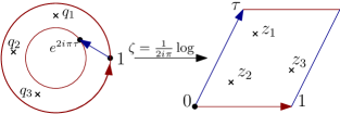
Figure 4. The elliptic curve $\mathbb{T}_{\tau}$ with four marked points ($z_{0}=0$), represented as a parallelogramme with opposite sides identified. The $\mathfrak{a}$-cycle (resp. $\mathfrak{b}$-cycle) is in red (resp. blue). The standard mapping $\zeta=\frac{1}{2i\pi}\log:\mathbb{A}_{\tau}\to\mathbb{T}_{\tau}$ (defined away from the $\mathfrak{b}$-cut) gives the parametrisation of the $\mathfrak{a}$-cycle. The vector field $\partial_{\tau}$ generating the deformation of the complex structure is pulled-back to the annulus as $\frac{1}{2i\pi}q\partial_{q}$ (with $q=\zeta^{-1}=e^{2i\pi\tau}$).

We will be needing the Jacobi $\vartheta$-function and the Weierstrass $\wp$-function, with the Laurent expansions around $z=0$:

$$\frac{\vartheta^{\prime}(z;\tau)}{\vartheta(z;\tau)}=\frac{1}{z}+\frac{\vartheta^{\prime\prime\prime}(0;\tau)}{3\vartheta^{\prime}(0;\tau)}z-\sum_{n=1}^{\infty}G_{2n+2}(\tau)z^{2n+1};$$

$$\wp(z;\tau)=\frac{1}{z^{2}}+\sum_{n=1}^{\infty}(2n+1)G_{2n+2}(\tau)z^{2n},$$

where $G_{n}(\tau)=\sum_{(k,l)\in\mathbb{Z}^{2}\setminus\{(0,0)\}}(k+l\tau)^{-n}$ is the Eisenstein series for $n\;\geqslant\;3$ and $\tau\in\mathbb{H}$.

The parametrisation of the $\mathfrak{a}$-cycle is $\zeta:\mathbb{S}^{1}\to[0,1),\,z\mapsto\frac{1}{2i\pi}\log z$, which extends to an embedding of the straight annulus $\mathbb{A}_{\tau}$ to the domain $\mathbb{T}_{\tau}$ (away from the $\mathfrak{b}$-cut). The vector field $\partial_{\tau}$ generating the deformation of the complex structure is represented by the constant vector field $\partial_{z}$ on the $\mathfrak{a}$-cycle: the pairing of a quadratic differential $q\mathrm{d}z^{2}$ is $(q\mathrm{d}z^{2},\partial_{\tau})=\frac{1}{2i\pi}\int_{0}^{1}q\mathrm{d}z$. The basis of quadratic differentials dual to the frame $(\partial_{\tau},\partial_{z_{1}},...,\partial_{z_{m}})$ is then

$$q_{-2}(z):=2i\pi;$$

$$q_{-1,j}(z):=\frac{\vartheta^{\prime}(z-z_{j};\tau)}{\vartheta(z-z_{j};\tau)}-\frac{\vartheta^{\prime}(z;\tau)}{\vartheta(z;\tau)},\qquad 1\;\leqslant\;j\;\leqslant\;m.$$

Indeed, one checks from the Laurent expansions above that $q_{-1,j}$ has a simple pole at $z_{j}$ (and $z_{0}=0$), with unit residue at $z_{j}$. Using the value $\int_{0}^{1}\wp(z;\tau)\mathrm{d}z=\frac{\vartheta^{\prime\prime\prime}(0;\tau)}{3\vartheta^{\prime}(0;\tau)}$, the connection in $\mathscr{L}^{\boldsymbol{\Delta}}$ is given by the quadratic differential

$$q_{\boldsymbol{\Delta}}(z):=\sum_{j=0}^{m}\Delta_{j}\left(\wp(z-z_{j};\tau)-\frac{\vartheta^{\prime\prime\prime}(0;\tau)}{3\vartheta^{\prime}(0;\tau)}\right).$$

It has a double pole at $z_{j}$ with residue $\Delta_{j}$, and it vanishes against the frame $(\partial_{\tau},\partial_{z_{1}},...,\partial_{z_{m}})$ since its $\mathfrak{a}$-period vanishes and it has no simple poles.

Now, we have the following Laurent expansions around 0:

$$q_{\boldsymbol{\Delta}}(z)=\Delta_{0}\left(\frac{1}{z^{2}}-\frac{\vartheta^{\prime\prime\prime}(0;\tau)}{\vartheta^{\prime}(0;\tau)}+\sum_{n=1}^{\infty}(2n+1)G_{2n+2}z^{2n}\right)-\sum_{j=1}^{m}\Delta_{j}\left(\frac{\vartheta^{\prime\prime\prime}(0;\tau)}{\vartheta^{\prime}(0;\tau)}-\sum_{n=0}^{\infty}\frac{(-1)^{n}}{n!}\wp^{(n)}(z_{j};\tau)z^{n}\right),$$

$$q_{-1,j}(z)=-\frac{1}{z}-\frac{\vartheta^{\prime}(z_{j};\tau)}{\vartheta(z_{j};\tau)}+\frac{\vartheta^{\prime\prime\prime}(0;\tau)}{3\vartheta^{\prime}(0;\tau)}z+\sum_{n=1}^{\infty}G_{2n+2}z^{2n+1}+\sum_{n=1}^{\infty}\frac{(-1)^{n}}{(n-1)!}\wp^{(n-1)}(z_{j};\tau)z^{n}.$$

The expression for the differential operators $\mathcal{L}_{n}=\mathcal{L}_{n}^{(0)}$ is then obtained by evaluating the pairings of $z^{n+1}\partial_{z}$ against the dual basis of quadratic differentials and the connection $q_{\boldsymbol{\Delta}}$, i.e. by looking at the Laurent expansions at 0. For $n\;\geqslant\;1$ and $j=1,...,m$, we find

$$\mathcal{L}_{-1}^{(j)}:=\partial_{z_{j}};\qquad\mathcal{L}_{-1}=0;$$ (5.1)

$$\mathcal{L}_{-2}:=2i\pi\partial_{\tau}-\sum_{j=1}^{m}\frac{\vartheta^{\prime}(z_{j};\tau)}{\vartheta(z_{j};\tau)}\partial_{z_{j}}-\Delta_{\alpha_{0}}\frac{\vartheta^{\prime\prime\prime}(0;\tau)}{3\vartheta^{\prime}(0;\tau)}-\sum_{j=1}^{m}\Delta_{\alpha_{j}}\left(\frac{\vartheta^{\prime\prime\prime}(0;\tau)}{3\vartheta^{\prime}(0;\tau)}-\wp(z_{j};\tau)\right),$$

$$\mathcal{L}_{-2n-2}:=\Delta_{\alpha_{0}}(2n+1)G_{2n+2}(\tau)+\frac{1}{(2n)!}\sum_{j=1}^{m}\left(\wp^{(2n-1)}(z_{j};\tau)\partial_{z_{j}}+\Delta_{\alpha_{j}}\wp^{(2n)}(z_{j};\tau)\right),$$

$$\mathcal{L}_{-2n-1}:=\frac{1}{(2n-1)!}\sum_{j=1}^{m}\left(\left((2n-1)G_{2n}(\tau)-\wp^{(2n-2)}(z_{j};\tau)\right)\partial_{z_{j}}-\Delta_{\alpha_{j}}\wp^{(2n-1)}(z_{j};\tau)\right).$$

Note that for $n>2$, $\mathcal{L}_{-n}$ has no derivative in the modulus $\tau$. This is due to the fact that $\wp^{(n-3)}$ has a unique pole of order $n-1$ at 0 and vanishing residue, so the deformation generated by $z_{0}^{-n+1}\partial_{z_{0}}$ is equivalent to the one generated by germs of holomorphic vector fields at the marked points. These vector fields only move the marked points but don’t change the complex structure.

As an application, we can write the BPZ equation at level 2 on the torus with two marked points at $(0,z)$. We put a degenerate weight $\alpha_{0}\in\{\alpha_{1,2},\alpha_{2,1}\}$ at $z$ and an arbitrary weight $\alpha$ at 0. The BPZ operator is then given by

$$\frac{1}{\alpha_{0}^{2}}\mathcal{L}_{-1}^{2}+\mathcal{L}_{-2}=2i\pi\partial_{\tau}+\frac{1}{\alpha_{0}^{2}}\partial_{uu}^{2}-\frac{\vartheta^{\prime}(u;\tau)}{\vartheta^{\prime}(u;\tau)}\partial_{u}-\Delta_{\alpha_{0}}\frac{\vartheta^{\prime\prime\prime}(0;\tau)}{3\vartheta^{\prime}(0;\tau)}-\Delta_{\alpha_{1}}\left(\frac{\vartheta^{\prime\prime\prime}(0;\tau)}{3\vartheta^{\prime}(0;\tau)}-\wp(u;\tau)\right).$$

Remark 9.

On $\mathcal{T}_{\mathbb{T},1}^{\epsilon}$, we have a Virasoro frame $(\mathbf{v}_{-2},\mathbf{v}_{n})_{n\;\geqslant\;0}$, and from the Laurent expansions, we see that the dual basis is expressed in terms of derivatives of the Weierstrass $\wp$-functions. This allows us to expand $\partial_{\tau}$ in the Virasoro frame to get

$$2i\pi\partial_{\tau}=\left(\frac{1}{z}+\frac{\vartheta^{\prime\prime\prime}(0;\tau)}{3\vartheta^{\prime}(0;\tau)}z-\sum_{n=1}^{\infty}G_{2n+2}z^{2n+1}\right)\partial_{z}=\frac{\vartheta^{\prime}(z;\tau)}{\vartheta(z;\tau)}\partial_{z}.$$

5.3. Hyperbolic surfaces

In this section, we suppose that $\Sigma$ has genus $\mathbf{g}\;\geqslant\;2$. Every point $(\Sigma,J)\in\mathcal{T}_{\Sigma}$ can be represented as $\Gamma\backslash\mathbb{D}$ for some Fuchsian subgroup $\Gamma$ of $\mathrm{PSL}_{2}(\mathbb{R})$. The local inverses of the canonical projection $\mathbb{D}\to\Gamma\backslash\mathbb{D}$ give an atlas with transition functions in $\mathrm{PSL}_{2}(\mathbb{R})$, so we get a canonical projective structure (it is known as the Fuchsian projectie structure). We pick a fundamental domain $F$ and use the standard coordinate $z$ inherited from $\mathbb{D}$. Let $z_{0},z_{1},...,z_{m}\in F$ be the unique representatives of the marked points in $F$ (again, we identify the marked points with the canonical local coordinate).

Let $\mathcal{G}$ be a connected graph encoding a pair of pants decomposition. In each homotopy class of curves in $\mathcal{G}$, there is a unique geodesic representative (for the hyperbolic metric). Since geodesics are circle arcs in $\mathbb{D}$ (which are preserved by Möbius transformations), the geodesic representative of the pair of pants decomposition is compatible with the Fuchsian projective structure. Moreover, the plumbing coordinates induced from these geodesics define a new projective structure [Dum09, Section 4]; namely, we get a local section of the bundle of projective structure over the plumbing chart. Let $(\partial_{\tau_{1}},...,\partial_{\tau_{3\mathbf{g}-3}})$ be the corresponding frame, i.e. $\partial_{\tau_{j}}$ generates the plumbing deformation from the $j^{\text{th}}$ curve. Then, $(\partial_{\tau_{1}},...,\partial_{\tau_{3\mathbf{g}-3}},\partial_{z_{0}},...\partial_{z_{m}})$ is a local holomorphic frame on $T\mathcal{T}_{\Sigma,m}$. Let $(q_{-2,1},...,q_{-2,3\mathbf{g}-3},q_{-1,0},...,q_{-1,m})$ be the dual frame on $T^{*}\mathcal{T}_{\Sigma,m}$. The quadratic differential $q_{-2,k}$ is holomorphic on $(\Sigma,J)$ for each $k=1,...,3\mathbf{g}-3$, while $q_{-1,j}$ has a simple pole at $z_{j}$ and no other pole.

Let $\mathrm{Quad}_{2}^{\boldsymbol{\Delta}}(\Sigma\setminus\{\boldsymbol{z}\},J)$ be the subspace of $\mathrm{Quad}_{2}(\Sigma\setminus\{\boldsymbol{z}\},J)$ consisting of meromorphic quadratic differentials $q\mathrm{d}z^{2}$ on $(\Sigma,J)$ with double poles at the punctures (and no other poles), and expansion

$$q(z)=\frac{\Delta_{j}}{(z-z_{j})^{2}}+O((z-z_{j})^{-1}),$$

namely $\mathrm{Res}_{z_{j}}\,q\mathrm{d}z^{2}=\Delta_{j}$. The space $\mathrm{Quad}_{2}^{\boldsymbol{\Delta}}(\Sigma\setminus\{\boldsymbol{z}\},J)$ is an affine space of complex dimension $3\mathbf{g}-3+m+1$, modelled on $\mathrm{Quad}_{1}(\Sigma\setminus\{\boldsymbol{z}\},J)$. The collection of such spaces as $(\Sigma,J,\boldsymbol{z})$ varies in $\mathcal{T}_{\Sigma,m+1}$ defines an affine bundle $\mathrm{Quad}_{2}^{\boldsymbol{\Delta}}\to\mathcal{T}_{\Sigma,m+1}$. There exists a unique $q_{\boldsymbol{\Delta}}\in\mathrm{Quad}_{2}^{\boldsymbol{\Delta}}(\Sigma\setminus\{\boldsymbol{z}\},J)$ such that

$$(q_{\boldsymbol{\Delta}},\partial_{\tau_{k}})=(q_{\boldsymbol{\Delta}},\partial_{z_{j}})=0,\qquad\forall k=1,...,3\mathbf{g}-3,\,\forall j=0,...,m.$$

This $q_{\boldsymbol{\Delta}}$ is the connection in $\mathscr{L}^{\boldsymbol{\Delta}}$, and it defines a holomorphic section of $\mathrm{Quad}_{2}^{\boldsymbol{\Delta}}$. We write the Laurent expansions around $z_{0}$ in the coordinate $z$:

$$q_{-2,k}(z)=:\sum_{n=2}^{\infty}\varpi_{-2,k}^{n}(z-z_{0})^{n-2}; k=1,...,3\mathbf{g}-3$$

$$q_{-1,0}(z)=:\sum_{n=1}^{\infty}\varpi_{-1,j}^{n}(z-z_{0})^{n-2};$$

$$q_{-1,j}(z)=:\sum_{n=2}^{\infty}\varpi_{-1,j}^{n}(z-z_{0})^{n-2}; j=1,...,m$$

$$q_{\boldsymbol{\Delta}}(z)=:\frac{\Delta_{0}}{(z-z_{0})^{2}}+\sum_{n=1}^{\infty}\varpi_{\boldsymbol{\Delta}}^{n}(z-z_{0})^{n-2}.$$

The coefficients in these expansions are holomorphic on $\mathcal{T}_{\Sigma,m+1}$ since the quadratic differentials involved vary holomorphically on $\mathcal{T}_{\Sigma,m+1}$. The BPZ operators $\mathcal{L}_{-n}=\mathcal{L}_{-n}^{(0)}$ are then given for $n\;\geqslant\;2$ by

$$\mathcal{L}_{-n}=\sum_{k=1}^{3\mathbf{g}-3}\varpi_{-2,k}^{n}\partial_{\tau_{k}}+\sum_{j=0}^{m}\left(\varpi_{-1,j}^{n}\partial_{z_{j}}+\Delta_{j}\varpi_{\boldsymbol{\Delta}}^{n}\right),$$

which is the form written in (1.3).

Appendix A Martingales of the Ornstein-Uhlenbeck process

Let $(\Omega,(\mathcal{F}_{t})_{t\;\geqslant\;0},\mathbb{P})$ be a filtered probability space on which is defined a standard Brownian motion $(W_{t})_{t\;\geqslant\;0}$. The Ornstein-Uhlenbeck (OU) process with parameters $\kappa,\sigma>0$ is the solution to the SDE

$$\mathrm{d}U_{t}=-\kappa U_{t}\mathrm{d}t+\sigma\mathrm{d}W_{t}.$$

The process $M_{t}:=e^{\kappa t}U_{t}$ is a martingale and solves the SDE

$$\mathrm{d}M_{t}=\sigma e^{\kappa t}\mathrm{d}W_{t}.$$

Its quadratic variation is given by

$$[M]_{t}=\sigma^{2}\int_{0}^{t}e^{2\kappa s}\mathrm{d}s=\frac{\sigma^{2}}{\kappa}e^{\kappa t}\sinh(\kappa t).$$

For each $\varepsilon\in\mathbb{R}$, we can form the exponential martingale

$$\mathcal{E}_{\varepsilon}(t):=e^{\varepsilon M_{t}-\frac{\varepsilon^{2}}{2}[M]_{t}}.$$

The initial value is $\mathcal{E}_{\varepsilon}(0)=e^{\varepsilon U_{0}}$. This martingale is real analytic in $\varepsilon$, and we can write

$$\mathcal{E}_{\varepsilon}(t)=:\sum_{n=0}^{\infty}M_{n}(t)\frac{\varepsilon^{n}}{n!},$$

where each $M_{n}$ is a martingale. Explicitly, $M_{n}(t)=[M]_{t}^{n/2}\mathrm{He}_{n}(\frac{M_{t}}{[M]_{t}^{1/2}})$, where $\mathrm{He}_{n}$ is the $n^{\text{th}}$ Hermite polynomial. For instance, we have $M_{1}(t)=M_{t}$ and $M_{2}(t)=M_{t}^{2}-[M]_{t}$.

By the Girsanov transform, reweighting the measure by $e^{-\varepsilon U_{0}}\mathcal{E}_{\varepsilon}(t)$ amounts to the shift $M_{t}\mapsto M_{t}+\varepsilon[M]_{t}$, or equivalently $U_{t}\mapsto U_{t}+\frac{\varepsilon\sigma^{2}}{\kappa}\sinh(\kappa t)$. More precisely, we have for every measurable function $F:\mathcal{C}^{0}([0,t_{0}])\to\mathbb{R}$,

$$\mathbb{E}\left[\mathcal{E}_{\varepsilon}(t_{0})F\left((U_{t})_{0\;\leqslant\;t\;\leqslant\;t_{0}}\right)\right]=e^{\varepsilon U_{0}}\mathbb{E}\left[F\left(\left(U_{t}+\frac{\varepsilon\sigma^{2}}{\kappa}\sinh(\kappa t)\right)_{0\;\leqslant\;t\;\leqslant\;t_{0}}\right)\right].$$ (A.1)

The shifted process and the original one are mutually absolutely continuous up to finite $t_{0}$, but they are singular for $t_{0}=\infty$ (since the shifted process diverges to $\mathrm{sgn}(\varepsilon)\infty$ almost surely).

Appendix B The Virasoro algebra

For the reader’s convenience, we recall some notions and terminology from the representation theory of the Virasoro algebra. The main reference is [KRR13]. The interested reader will find more information on the structure of degenerate highest-weight modules in [Ast97].

The (complex) Witt algebra $\mathfrak{w}$ is the infinite dimensional Lie algebra of holomorphic vector fields in the neighbourhood of the unit circle $\mathbb{S}^{1}$. The commutation relations read

$$[v\partial_{z},w\partial_{z}]=(vw^{\prime}-v^{\prime}w)\partial_{z},\qquad\forall\,v\partial_{z},w\partial_{z}\in\mathfrak{w}.$$

It admits the generators $\mathbf{v}_{n}=-z^{n+1}\partial_{z}$, and the commutation relations for the generators is the familiar formula

$$[\mathbf{v}_{n},\mathbf{v}_{m}]=(n-m)\mathbf{v}_{n+m}.$$

The Witt algebra admits an $\mathfrak{sl}_{2}$-Lie subalgebra spanned by $\{\mathbf{v}_{-1},\mathbf{v}_{0},\mathbf{v}_{1}\}$: these are the polynomial vector fields on the Riemann sphere generating Möbius transformations.

The Virasoro cocycle is the 2-cocycle on $\mathfrak{w}$ given by

$$\omega(v\partial_{z},w\partial_{z}):=\frac{1}{24i\pi}\oint_{\mathbb{S}^{1}}v^{\prime\prime\prime}w\mathrm{d}z.$$ (B.1)

In terms of the generators, we have $(\mathbf{v}_{n},\mathbf{v}_{m})\mapsto\frac{1}{12}(n^{3}-n)\delta_{n,-m}$. The Virasoro algebra $\mathfrak{v}$ is the corresponding central extension of $\mathfrak{w}$. It is customary to write the generators $(L_{n})_{n\in\mathbb{Z}}$ and the central element $\mathbf{c}$, so that the commutation relations read:

$$[L_{n},L_{m}]=(n-m)L_{n+m}+\frac{\mathbf{c}}{12}(n^{3}-n)\delta_{n,-m};\qquad[L_{n},\mathbf{c}]=0.$$

From the commutation relations, we have a Lie subalgebra $\mathfrak{v}^{+}$ (resp. $\mathfrak{v}^{-}$) generated by $\{L_{n},\,n\;\geqslant\;1\}$ (resp. $\{L_{n},\,n\;\leqslant\;-1\}$). An integer partition is a non-decreasing sequence of integers with finitely many non-zero terms. The set of integer partitions is denoted $\mathcal{T}$. By the Poincaré-Birkhoff-Witt theorem, the universal enveloping algebra $\mathcal{U}(\mathfrak{v}^{-})$ admits a linear basis $\{L_{-\nu}=L_{-\nu_{1}}L_{-\nu_{2}}\cdots L_{-\nu_{\ell}}|\,\nu=(\nu_{1},...,\nu_{\ell})\in\mathcal{T}\}$. The level of a partition is the number $|\nu|=\sum_{n=1}^{\infty}\nu_{n}$ partitioned by $\nu$.

A Virasoro module is a vector space $V$ together with a bilinear map $\rho:\mathfrak{v}\times V\to V,\,(L_{n},v)\mapsto L_{n}\cdot v$ such that $[L_{n},L_{m}]\cdot v=L_{n}\cdot(L_{m}\cdot v)-L_{m}\cdot(L_{n}\cdot v)$. We will always consider modules such that there exists $c_{\mathrm{L}}\in\mathbb{C}$ such that $\mathbf{c}\cdot v=c_{\mathrm{L}}v$ for all $v\in V$. The scalar $c_{\mathrm{L}}$ is called the central charge. A module $V$ is irreducible if it contains no non-trivial proper submodule.

A vector $v\in V$ is a highest-weight vector of (highest) weight $\Delta\in\mathbb{C}$ if $L_{n}\cdot v=0$ for all $n\;\geqslant\;1$ and $L_{0}\cdot v=\Delta v$. A module $V$ is a highest-weight module of (highest) weight $\Delta$ if $V=\mathrm{span}\{L_{-\nu}\cdot v|\,\nu\in\mathcal{T}\}$ for some highest-weight vector $v$. Namely, $V$ is obtained by acting on $v$ with $\mathcal{U}(\mathfrak{v}^{-})$. From the commutation relations, $L_{-\nu}\cdot v$ is an eigenstate of $L_{0}$ with eigenvalue $\Delta+|\nu|$. This gives a grading of $V$ by the level: $V=\oplus_{N\in\mathbb{N}}V_{N}$. The space $V_{0}$ is one-dimensional (spanned by $v$), and the vectors at level $N>0$ are the descendants of $v$. It is customary to parametrise the central charge and the highest weight with the so-called Liouville parameters $\gamma,\alpha\in\mathbb{C}$:

$$c_{\mathrm{L}}=1+6Q^{2};\qquad\Delta=\frac{\alpha}{2}(Q-\frac{\alpha}{2}),$$

and $Q=\frac{\gamma}{2}+\frac{2}{\gamma}$. Notice that the map $(\gamma,\alpha)\mapsto(c_{\mathrm{L}},\Delta)$ is not one-to-one, since $\Delta$ is invariant under $\alpha\mapsto 2Q-\alpha$ and $c_{\mathrm{L}}$ is invariant under $\gamma\mapsto\frac{4}{\gamma}$.

A Verma module is a highest-weight module such that the canonical map $\mathcal{U}(\mathfrak{v}^{-})\to V,\,L_{-\nu}\mapsto L_{-\nu}\cdot v$ is a linear isomorphism. For each $c_{\mathrm{L}},\Delta\in\mathbb{C}$, the Verma module with central charge $c_{\mathrm{L}}$ and highest-weight $\Delta$ exists and is unique up to isomorphism. It is denoted $M(c_{\mathrm{L}},\Delta)$. Any highest-weight module $V$ is isomorphic to the quotient of $M(c_{\mathrm{L}},\Delta)$ by a proper submodule. We then have a canonical projection $M(c_{\mathrm{L}},\Delta)\to V$ sending $L_{-\nu}$ to the descendant state $L_{-\nu}\cdot v\in V$. It is a fact that any submodule of a highest-weight module is itself a highest-weight module. A vector $w\in V$ is singular if it is both a descendant and a highest-weight vector. Any non-zero singular vector generates a highest-weight module, so $M(c_{\mathrm{L}},\Delta)$ is irreducible if and only if it contains no non-zero singular vectors. The maximal proper submodule $I(c_{\mathrm{L}},\Delta)$ is the (unique) proper submodule containing all other proper submodules. The quotient

$$V(c_{\mathrm{L}},\Delta):=M(c_{\mathrm{L}},\Delta)/I(c_{\mathrm{L}},\Delta)$$

is irreducible.

For each $\nu,\nu^{\prime}\in\mathcal{T}$ with the same level $N$, $L_{\nu^{\prime}}\cdot(L_{-\nu}\cdot v)$ is at level zero, so we have $L_{\nu^{\prime}}\cdot(L_{-\nu}\cdot v)=S_{N}(\nu,\nu^{\prime})v$ for some scalar $S_{N}(\nu,\nu^{\prime})$. The matrix $(S_{N}(\nu,\nu^{\prime}))_{|\nu|=|\nu^{\prime}|=N}$ is called the Shapovalov matrix and it defines a bilinear form on the level-$N$ subspace of $V(c_{\mathrm{L}},\Delta)$. It is non-degenerate for all $N\in\mathbb{N}$ if and only if $V(c_{\mathrm{L}},\Delta)$ is irreducible. More precisely, $I(c_{\mathrm{L}},\Delta)$ coincides with the kernel of the Shapovalov form. The Kac determinant formula gives an explicit expression for the determinant of the Shapovalov matrix

$$\det S_{N}\propto\prod_{1\;\leqslant\;rs\;\leqslant\;N}(\Delta-\Delta_{r,s})^{p(N-rs)},$$

where $\Delta_{r,s}$ is the weight corresponding to $\alpha_{r,s}=Q-\frac{\gamma}{2}r-\frac{2}{\gamma}s$, with $r,s\in\mathbb{N}^{*}$. In particular, the Shapovalov form is degenerate at some level if and only if $\alpha$ belongs to the Kac table $kac=kac^{-}\sqcup kac^{+}$, with $kac^{\pm}=(1\pm\mathbb{N}^{*})\frac{\gamma}{2}+(1\pm\mathbb{N}^{*})\frac{2}{\gamma}$. The two sets satisfy $kac^{-}=2Q-kac^{+}$, and $kac^{-}\subset\mathbb{R}_{-}$.

References

- [ABO18] Jørgen Ellegaard Andersen, Gaëtan Borot, and Nicolas Orantin. Modular functors, cohomological field theories, and topological recursion. In Topological recursion and its influence in analysis, geometry, and topology, volume 100 of Proc. Sympos. Pure Math., pages 1–58. Amer. Math. Soc., Providence, RI, 2018.
- [Ang23] Morris Ang. Liouville conformal field theory and the quantum zipper. arXiv e-prints, page arXiv:2301.13200, January 2023.
- [ARS21] Morris Ang, Guillaume Remy, and Xin Sun. FZZ formula of boundary Liouville CFT via conformal welding. arXiv e-prints, page arXiv:2104.09478, April 2021.
- [ARSZ23] Morris Ang, Guillaume Remy, Xin Sun, and Tunan Zhu. Derivation of all structure constants for boundary Liouville CFT. arXiv e-prints, page arXiv:2305.18266, May 2023.
- [Ast97] A. Astashkevich. On the structure of Verma modules over Virasoro and Neveu-Schwarz algebras. Comm. Math. Phys., 186(3):531–562, 1997.
- [BB10] A. Belavin and V. Belavin. Higher equations of motion in boundary Liouville field theory. J. High Energy Phys., (2):010, 18, 2010.
- [Ber17] Nathanaël Berestycki. An elementary approach to Gaussian multiplicative chaos. Electron. Commun. Probab., 22:Paper No. 27, 12, 2017.
- [BGK+23a] Guillaume Baverez, Colin Guillarmou, Antti Kupiainen, Rémi Rhodes, and Vincent Vargas. The conformal blocks of Liouville conformal field theory. in preparation, 2023.
- [BGK+23b] Guillaume Baverez, Colin Guillarmou, Antti Kupiainen, Rémi Rhodes, and Vincent Vargas. The Virasoro structure and the scattering matrix for Liouville conformal field theory. to appear in Probability and Mathematical Physics, 2023.
- [BPZ84] A.A. Belavin, A.M. Polyakov, and A.B. Zamolodchikov. Infinite conformal symmetry in two-dimensional quantum field theory. Nuclear Physics B, 241(2):333–380, 1984.
- [DFMS97] Philippe Di Francesco, Pierre Mathieu, and David Sénéchal. Conformal field theory. Graduate Texts in Contemporary Physics. Springer-Verlag, New York, 1997.
- [DKRV16] François David, Antti Kupiainen, Rémi Rhodes, and Vincent Vargas. Liouville quantum gravity on the Riemann sphere. Comm. Math. Phys., 342(3):869–907, 2016.
- [DMS14] Bertrand Duplantier, Jason Miller, and Scott Sheffield. Liouville quantum gravity as a mating of trees. To appear in Astérisque, page arXiv:1409.7055, Sep 2014.
- [DRV16] François David, Rémi Rhodes, and Vincent Vargas. Liouville quantum gravity on complex tori. J. Math. Phys., 57(2):022302, 25, 2016.
- [Dum09] David Dumas. Complex projective structures. In Handbook of Teichmüller theory. Vol. II, volume 13 of IRMA Lect. Math. Theor. Phys., pages 455–508. Eur. Math. Soc., Zürich, 2009.
- [EO87] Tohru Eguchi and Hirosi Ooguchi. Conformal and current algebras on a general riemann surface. Nuclear Physics B, 282:308–328, 1987.
- [FB01] Edward Frenkel and David BenZvi. Vertex algebras and algebraic curves, volume 88 of Mathematical Surveys and Monographs. American Mathematical Society, Providence, RI, 2001.
- [Fre92] Edward Frenkel. Determinant formulas for the free field representations of the Virasoro and Kac-Moody algebras. Phys. Lett. B, 286(1-2):71–77, 1992.
- [Fre07] Edward Frenkel. Lectures on the Langlands program and conformal field theory. In Frontiers in number theory, physics, and geometry. II, pages 387–533. Springer, Berlin, 2007.
- [FS87] Daniel Friedan and Stephen Shenker. The analytic geometry of two-dimensional conformal field theory. Nuclear Phys. B, 281(3-4):509–545, 1987.
- [FZZ00] V. Fateev, A. Zamolodchikov, and Al. Zamolodchikov. Boundary Liouville Field Theory I. Boundary State and Boundary Two-point Function. arXiv e-prints, pages hep–th/0001012, January 2000.
- [GKRV21] Colin Guillarmou, Antti Kupiainen, Rémi Rhodes, and Vincent Vargas. Segal’s axioms and bootstrap for Liouville Theory. arXiv e-prints, page arXiv:2112.14859, December 2021.
- [GKRV23] Colin Guillarmou, Antti Kupiainen, Rémi Rhodes, and Vincent Vargas. Conformal bootstrap in Liouville Theory. to appear in Acta Mathematica, 2023.
- [GRSS20] Promit Ghosal, Guillaume Remy, Xin Sun, and Yi Sun. Probabilistic conformal blocks for Liouville CFT on the torus. arXiv e-prints, page arXiv:2003.03802, March 2020.
- [GRV19] Colin Guillarmou, Rémi Rhodes, and Vincent Vargas. Polyakov’s formulation of bosonic string theory. Publ. Math. Inst. Hautes Études Sci., 130:111–185, 2019.
- [GT12] Davide Gaiotto and Joerg Teschner. Irregular singularities in Liouville theory and Argyres-Douglas type gauge theories. Journal of High Energy Physics, 2012:1–79, 2012.
- [Kah85] Jean-Pierre Kahane. Sur le chaos multiplicatif. Ann. Sci. Math. Québec, 9(2):105–150, 1985.
- [KRR13] Victor G Kac, Ashok K Raina, and Natasha Rozhkovskaya. Bombay Lectures on Highest Weight Representations of Infinite Dimensional Lie Algebras. WORLD SCIENTIFIC, 2nd edition, 2013.
- [KRV19] Antti Kupiainen, Rémi Rhodes, and Vincent Vargas. Local conformal structure of Liouville quantum gravity. Comm. Math. Phys., 371(3):1005–1069, 2019.
- [KRV20] Antti Kupiainen, Rémi Rhodes, and Vincent Vargas. Integrability of Liouville theory: proof of the DOZZ formula. Ann. of Math. (2), 191(1):81–166, 2020.
- [McM00] Curtis T. McMullen. The moduli space of Riemann surfaces is Kähler hyperbolic. Ann. of Math. (2), 151(1):327–357, 2000.
- [Oik19] Joona Oikarinen. Smoothness of correlation functions in Liouville conformal field theory. Ann. Henri Poincaré, 20(7):2377–2406, 2019.
- [Rib14] Sylvain Ribault. Conformal field theory on the plane. arXiv e-prints, page arXiv:1406.4290, June 2014.
- [RV14] Rémi Rhodes and Vincent Vargas. Gaussian multiplicative chaos and applications: a review. Probab. Surv., 11:315–392, 2014.
- [RZ20] Guillaume Remy and Tunan Zhu. Integrability of boundary liouville conformal field theory. Communications in Mathematical Physics, 395:179 – 268, 2020.
- [Seg04] Graeme Segal. The definition of conformal field theory. In Topology, geometry and quantum field theory, volume 308 of London Math. Soc. Lecture Note Ser., pages 421–577. Cambridge Univ. Press, Cambridge, 2004.
- [Tes17] Joerg Teschner. A guide to two-dimensional conformal field theory. arXiv e-prints, page arXiv:1708.00680, August 2017.
- [Zam04] A. Zamolodchikov. Higher equations of motion in Liouville field theory. Int. J. Mod. Phys. A, 19S2:510–523, 2004.
- [Zhu20] Tunan Zhu. Higher order BPZ equations for Liouville conformal field theory. arXiv e-prints, page arXiv:2001.08476, January 2020.