Momentum Particle Maximum Likelihood

Abstract

Maximum likelihood estimation (MLE) of latent variable models is often recast as the minimization of a free energy functional over an extended space of parameters and probability distributions. This perspective was recently combined with insights from optimal transport to obtain novel particle-based algorithms for fitting latent variable models to data. Drawing inspiration from prior works which interpret ‘momentum-enriched’ optimization algorithms as discretizations of ordinary differential equations, we propose an analogous dynamical-systems-inspired approach to minimizing the free energy functional. The result is a dynamical system that blends elements of Nesterov’s Accelerated Gradient method, the underdamped Langevin diffusion, and particle methods. Under suitable assumptions, we prove that the continuous-time system minimizes the functional. By discretizing the system, we obtain a practical algorithm for MLE in latent variable models. The algorithm outperforms existing particle methods in numerical experiments and compares favourably with other MLE algorithms.

1 Introduction

In this work, we study parameter estimation for (probabilistic) latent variable models $p_{\theta}\left(y,x\right)$ with parameters $\theta\in\mathbb{R}^{d_{\theta}}$, unobserved (or latent) variables $x\in\mathbb{R}^{d_{x}}$, and observed variables $y\in\mathbb{R}^{d_{y}}$ (which we treat as fixed throughout). The type II maximum likelihood approach (Good, , 1983) estimates $\theta$ by maximizing the marginal likelihood $p_{\theta}\left(y\right):=\int p_{\theta}\left(y,x\right)\,\mathrm{d}x$. However, for most models of practical interest, the integral has no known closed-form expressions and we are unable to optimize the marginal likelihood directly.

This issue is often overcome (e.g., Neal and Hinton, (1998)) by constructing an objective defined over an extended space, and whose optima are in one-to-one correspondence with those of the MLE problem. To this end, we define the ‘free energy’ functional:

$$\mathcal{E}\left(\theta,q\right):=\int\log\left(\frac{q\left(x\right)}{p_{\theta}\left(y,x\right)}\right)q\left(x\right)\,\mathrm{d}x.$$ (1)

The infimum of $\mathcal{E}$ over the extended space $\mathbb{R}^{d_{\theta}}\times\mathcal{P}(\mathbb{R}^{d_{x}})$ (where $\mathcal{P}(\mathbb{R}^{d_{x}})$ denotes the space of probability distributions over $\mathbb{R}^{d_{x}}$) coincides with negative of the log marginal likelihood’s supremum:

$$\mathcal{E}^{*}:=\inf_{(\theta,q)}\mathcal{E}(\theta,q)=-\sup_{\theta\in\mathbb{R}^{d_{\theta}}}\log p_{\theta}(y).$$ (2)

To see why, note that

$$\mathcal{E}\left(\theta,q\right)=-\log p_{\theta}\left(y\right)+\mathsf{KL}\left(q,p_{\theta}\left(\cdot\mid y\right)\right),$$ (3)

where $\mathsf{KL}$ denotes the Kullback-Leibler divergence and $p_{\theta}(\cdot|y):=p_{\theta}(y,\cdot)/p_{\theta}(y)$ the posterior distribution. So, if $(\theta^{*},q^{*})$ minimizes the free energy, then $\theta^{*}$ maximizes the marginal likelihood and $q^{*}(\cdot)=p_{\theta^{*}}(\cdot|y)$. In other words, by minimizing the free energy, we solve our MLE problem.

This perspective motivates the search for practical procedures that minimize the free energy $\mathcal{E}$. One such example is the classical EM algorithm applicable to models for which the posterior distributions $p_{\theta}\left(\cdot|y\right)$ are available in closed form. As shown in Neal and Hinton, (1998), its iterates coincide with those of coordinate descent applied to the free energy $\mathcal{E}$. Recently, Kuntz et al., (2023) sought analogues of gradient descent (GD) applicable to the free energy $\mathcal{E}$. In particular, building on ideas popular in optimal transport (e.g., see Ambrosio et al., (2005)), they identified an appropriate notion for the free energy’s gradient $\nabla\mathcal{E}$, discretized the corresponding gradient flow $(\dot{\theta}_{t},\dot{q}_{t})=-\nabla\mathcal{E}(\theta_{t},q_{t})$, and obtained a practical algorithm they called particle gradient descent (PGD).

In optimization, GD is well-known to be suboptimal: other practical first-order methods achieve better worst-case convergence guarantees and practical performance (Nemirovskij and Yudin, , 1983; Nesterov, , 1983). A common feature among algorithms that achieve the optimal ‘accelerated’ convergence rates is the presence of ‘momentum’ effects in the dynamics of the algorithm. Roughly speaking, if GD for a function $f$ is analogous to solving the ordinary differential equation (ODE)

$$\dot{\theta}_{t}=-\nabla_{\theta}f\left(\theta_{t}\right)$$ (4)

with $\nabla_{\theta}f$ denoting $f$’s Euclidean gradient, then a ‘momentum’ method is akin to solving a second-order ODE like

$$\dot{\theta}_{t} =\eta m_{t},\quad\dot{m}_{t}=-\gamma\eta m_{t}-\nabla_{\theta}f\left(\theta_{t}\right),$$ (5)

where $\gamma,\eta$ denote positive hyperparameters (Su et al., , 2014; Wibisono et al., , 2016). In the context of machine learning, Sutskever et al., (2013) demonstrated empirically that incorporating momentum effects into stochastic gradient descent (SGD) often has substantial benefits such as eliminating the performance gap between standard SGD and competing ‘Hessian-free’ deterministic methods based on higher-order differential information (Martens, , 2010).

Given the successes of momentum methods, it is natural to ask whether PGD can be similarly accelerated. In this work, we affirmatively answer this question. Our contributions are: (1) we construct a continuous-time flow that incorporates momentum effects into the gradient flow studied in Kuntz et al., (2023); (2) we derive a discretization that outperforms PGD and compares competitively against other methods. As theoretical contributions: (3) we prove in Proposition 3.1 the existence and uniqueness of the flow’s solutions; (4) under suitable conditions, we show in Theorem 4.1 that the flow converges to $\mathcal{E}$’s minima; and, (5) we asymptotically justify in Proposition 5.1 the particle approximations we use when discretizing the flow. The proofs of Proposition 3.1 and Proposition 5.1 require generalizations of proofs pertaining to McKean-Vlasov SDEs, and the proof of Theorem 4.1 is a generalization of the Ma et al., (2021)’s convergence argument. These may be of independent interest for future works that operate in the extended space $\mathbb{R}^{d_{\theta}}\times\mathcal{P}(\mathbb{R}^{d_{x}})$.

The structure of this manuscript is as follows: in Section 2, we review gradient flows on the Euclidean space $\mathbb{R}^{d_{\theta}}$, probability space $\mathcal{P}(\mathbb{R}^{d_{x}})$, and extended space $\mathbb{R}^{d_{\theta}}\times\mathcal{P}(\mathbb{R}^{d_{x}})$. We also review momentum methods on $\mathbb{R}^{d_{\theta}}$ and $\mathcal{P}(\mathbb{R}^{d_{x}})$. In Section 3, we describe how momentum can be incorporated into the gradient flow on $\mathbb{R}^{d_{\theta}}\times\mathcal{P}(\mathbb{R}^{d_{x}})$, resulting in a dynamical system we refer to as the ‘momentum-enriched flow’. In Section 4, we establish the flow’s convergence. In Section 5, we discretize the flow and obtain an MLE algorithm we refer to as Momentum Particle Descent (MPD). In Section 6, we demonstrate empirically the efficacy of our method and study the effects of various design choices. As a large-scale experiment, we benchmark our proposed method for training Variational Autoencoders (Kingma and Welling, , 2014) against current methods for training latent variable models. We conclude in Section 7 with a discussion of our results, their limitations, and future work.

2 Background

Our goal is to incorporate momentum into the gradient flow on the extended space $\mathbb{R}^{d_{\theta}}\times\mathcal{P}(\mathbb{R}^{d_{x}})$ considered in Kuntz et al., (2023) and obtain an algorithm for type II MLE that outperforms PGD. We begin by surveying the standard gradient flows on $\mathbb{R}^{d_{\theta}}\times\mathcal{P}(\mathbb{R}^{d_{x}})$’s component spaces and how momentum is incorporated in those settings.

2.1 Gradient Flows on $\mathbb{R}^{d}$ and their Acceleration

Given a differentiable function $f:\mathbb{R}^{d}\to\mathbb{R}$, $f$’s Euclidean gradient flow is (4). Discretizing (4) in time using a standard forward Euler integrator yields GD. As observed in (Su et al., , 2014; Shi et al., , 2021), algorithms such as Nesterov, (1983)’s accelerated gradient (NAG) that achieve the optimal convergence rates are instead obtained by discretising the second-order ODE (5); c.f. Section I.2. This ODE models the evolution of a kinetic particle with both position and momentum. In particular, for convex quadratic $f$, (5) reproduces the dynamics of a damped harmonic oscillator (McCall, , 2010). Hence, the ODE’s hyperparameters have intuitive interpretations: $\eta^{-1}$ represents the particle’s mass and $\gamma$ determines the damping’s strength.

We can rewrite (5) concisely as

$$(\dot{\theta}_{t},\dot{m}_{t})=-\mathsf{D}_{\gamma}\nabla_{\left(\theta,m\right)}f_{\eta}\left(\theta_{t},m_{t}\right),$$ (6)

where $f_{\eta}$ denotes the ‘Hamiltonian function’ and $\mathsf{D}_{\gamma}$ the ‘damping matrix’:

$$f_{\eta}\left(\theta,m\right)=f\left(\theta\right)+\frac{\eta}{2}\|m\|^{2},\enskip\mathsf{D}_{\gamma}:=\left(\begin{array}[]{cc}0_{d}&-I_{d}\\ I_{d}&\gamma I_{d}\end{array}\right).$$ (7)

In other words, (5) is a ‘damped’ or ‘conformal’ Hamiltonian flow (McLachlan and Perlmutter, , 2001; Maddison et al., , 2018). In particular, we can interpret NAG as a discretisation of $F_{\eta}$’s ‘$\gamma$-damped Hamiltonian flow’ (Wibisono et al., , 2016; Wilson et al., , 2016).

2.2 Gradient Flows on $\mathcal{P}\left(\mathbb{R}^{d}\right)$ and their Acceleration

We can follow a similar program to solve optimization problems over $\mathcal{P}\left(\mathbb{R}^{d}\right)$. To do so, we require an analogue of the Euclidean gradient $\nabla_{\theta}f$ for (differentiable) functionals $f$ on $\mathbb{R}^{d}$ applicable to (sufficiently-regular) functionals $F$ on $\mathcal{P}(\mathbb{R}^{d})$. One way of defining $\nabla_{\theta}f(\theta)$ at a given point $\theta$ is as the unique vector satisfying

$$f(\theta^{\prime})=f\left(\theta\right)+\langle\nabla_{\theta}f\left(\theta\right),\theta^{\prime}-\theta\rangle+o(\mathsf{d}_{E}(\theta,\theta^{\prime})),$$ (8)

where $\left\langle{\cdot},{\cdot}\right\rangle$ and $\mathsf{d}_{E}$ denote the Euclidean inner product and metric related by the formula

$$\mathsf{d}_{E}(\theta,\theta^{\prime})^{2}=\inf_{\lambda}\int_{0}^{1}\left\langle{\lambda_{t}},{\lambda_{t}}\right\rangle\,\mathrm{d}t,$$ (9)

where the infimum is taken over all (sufficiently-regular) curves $\lambda:[0,1]\to\mathbb{R}^{d}$ connecting $\theta$ and ${\theta}^{\prime}$. Roughly speaking, we can reverse this process to define $F$’s gradient for a given metric on $\mathcal{P}(\mathbb{R}^{d})$. Here, we focus on the Wasserstein-2 metric $\mathsf{W}_{2}$ for which (9)’s analogue is the Benamou-Brenier formula (Peyré and Cuturi, , 2019, Eq.7.2):

$$\mathsf{W}_{2}(q,q^{\prime})^{2}=\inf_{\rho}\int_{0}^{1}g_{\rho_{t}}(\dot{\rho}_{t},\dot{\rho}_{t})\,\mathrm{d}t$$

where the infimum is taken over all (sufficiently-regular) curves $\rho:[0,1]\to\mathbb{R}^{d}$ connecting $q$ and $\tilde{q}$ and

$$g_{q}(m,m^{\prime}):=\int\left\langle{v(x)},{v^{\prime}(x)}\right\rangle q(x)\mathrm{d}x,$$

where $v$ and $v^{\prime}$ solve the respective continuity equation, i.e., $m=-\nabla_{x}\cdot(qv),\quad m^{\prime}=-\nabla_{x}\cdot(qv^{\prime}).$ Then, replacing $(\theta,\theta^{\prime},f,\nabla_{\theta},\left\langle{\cdot},{\cdot}\right\rangle,\mathsf{d}_{E})$ with $(q,q^{\prime},F,\nabla_{q},g_{q}(\cdot,\cdot),$ $\mathsf{W}_{2})$ in (8) and solving for $\nabla_{q}F$, we obtain

$$\nabla_{q}F\left(q\right)=-\nabla_{x}\cdot\left(q\nabla_{x}\delta_{q}F\left[q\right]\right),$$

where $\delta_{q}F[q]:\mathbb{R}^{d}\to\mathbb{R}$ denotes the functional’s first variation: the function satisfying

$${F}\left(q+\varepsilon\chi\right)={F}\left(q\right)+\varepsilon\int\delta_{q}F\left[q\right]\left(x\right)\,\chi(x)\,\mathrm{d}x+o(\varepsilon)$$

for all (sufficiently-regular) $\chi:\mathbb{R}^{d}\to\mathbb{R}$ s.t. $\int\chi(x)\mathrm{d}x=0$. This is, of course, not the only choice; other metrics induce other ‘geometries’ and lead to other algorithms (e.g., see Duncan et al., (2023); Liu, (2017); Sharrock and Nemeth, (2023) for the Stein case). For a more rigorous presentation of these concepts, see Section C.1 and references therein.

We can now define $F$’s Wasserstein gradient flow just as in the Euclidean case (except we have a PDE rather than an ODE): $\dot{q}_{t}=-\nabla_{q}F\left(q_{t}\right).$ A well-known example of such a flow is that for which $F(\cdot):=\mathsf{KL}\left(\cdot,p\right)$ for a fixed $p$ in $\mathcal{P}\left(\mathbb{R}^{d}\right)$. In this case, $\delta_{q}F\left[q\right]=\log(q/p)$ and the flow reads $\dot{q}_{t}=\nabla_{x}\cdot\left(q_{t}\nabla_{x}\log(q_{t}/p)\right).$ As noted in Jordan et al., (1998), this is the Fokker-Planck equation satisfied by the law of the overdamped Langevin SDE with invariant measure $p$: $\mathrm{d}X_{t}=\nabla_{x}\ell\left(X_{t}\right)\,\mathrm{d}t+\sqrt{2}\,\mathrm{d}W_{t},$ where $\ell(x):=\log p(x)$ and $(W_{t})_{t\geq 0}$ denotes the standard Wiener process. For this reason, papers such as Wibisono, (2018); Ma et al., (2021) view the overdamped Langevin algorithm obtained by discretizing this SDE using the Euler-Maruyama scheme as an analogue of GD for $F$.

Ma et al., (2021) go a step further and search for ‘accelerated’ methods for minimizing $F$. To do so, they consider distributions over the momentum-enriched space $\mathbb{R}^{2d}$ rather than $\mathbb{R}^{d}$ and they replace $F$ on $\mathcal{P}(\mathbb{R}^{d})$ with the following ‘Hamiltonian’ on $\mathcal{P}(\mathbb{R}^{d}\times\mathbb{R}^{d}$):

$$F_{\eta}(\cdot):=\mathsf{KL}\left(\cdot,p(\mathrm{d}x)\otimes r_{\eta}(\mathrm{d}u)\right)\,,$$ (10)

where $\eta>0$ denotes a fixed hyperparameter, $r_{\eta}:=\mathcal{N}\left(0,\eta^{-1}I_{d}\right)$ a zero-mean $\eta^{-1}$-variance isotropic Gaussian distribution over the momentum variables $u$, and $p\otimes r_{\eta}$ the product measure. They then define the following $\mathcal{P}(\mathbb{R}^{2d})$-valued analogue of the $\gamma$-damped Hamiltonian flow (6):

$$\dot{q}_{t}=-\mathsf{D}_{\gamma}\nabla_{q}F_{\eta}(q_{t})=\nabla_{(x,u)}\cdot\left(q_{t}\mathsf{D}_{\gamma}\nabla_{(x,u)}\delta_{q}F_{\eta}\left[q_{t}\right]\right).$$ (11)

This is the Fokker-Planck equation satisfied by the law of the underdamped Langevin SDE:

$$\mathrm{d}X_{t}=\eta U_{t}\mathrm{d}t,\enskip\mathrm{d}U_{t}=[\nabla_{x}\ell(X_{t})-\gamma\eta U_{t}]\mathrm{d}t+\sqrt{2\gamma}\mathrm{d}W_{t}.$$ (12)

Discretizing the SDE, Ma et al., (2021) recover the underdamped Langevin algorithm (e.g., see Cheng et al., (2018)) and show that, under suitable conditions, it achieves faster convergence rates than the overdamped Langevin algorithm.

2.3 Gradient Flows on $\mathbb{R}^{d_{\theta}}\times\mathcal{P}\left(\mathbb{R}^{d_{x}}\right)$

To minimize a functional $\mathcal{E}$ on $\mathbb{R}^{d_{\theta}}\times\mathcal{P}\left(\mathbb{R}^{d_{x}}\right)$, we can follow steps analogous to those in the previous two sections. First, given a metric $\mathsf{d}$ on this space, we can define a gradient $\nabla\mathcal{E}$ w.r.t. $\mathsf{d}$ similarly as in the beginning of Section 2.2; cf. (Kuntz et al., , 2023, Appendix A). Setting $\mathsf{d}((\theta,q),(\theta^{\prime},q^{\prime})):=\sqrt{\mathsf{d}_{E}(\theta,\theta^{\prime})^{2}+\mathsf{W}_{2}(q,q^{\prime})^{2}}$, one finds that $\nabla\mathcal{E}=(\nabla_{\theta}\mathcal{E},\nabla_{q}\mathcal{E})$, and the corresponding flow reads

$$\dot{\theta}_{t} =-\nabla_{\theta}\mathcal{E}\left(\theta_{t},q_{t}\right),\quad\dot{q}_{t}=-\nabla_{q}\mathcal{E}\left(\theta_{t},q_{t}\right).$$

Kuntz et al., (2023) were interested in MLE of latent variable problems and set $\mathcal{E}$ to be the free energy in (1). In this case, the above reduces to

$$\dot{\theta}_{t}=\int\nabla_{\theta}\ell\left(\theta_{t},x\right)q_{t}\left(\mathrm{d}x\right),\enskip\dot{q}_{t}=\nabla_{x}\cdot\left(q_{t}\nabla_{x}\log\frac{q_{t}}{\rho_{\theta_{t}}}\right),$$

where $\rho_{\theta}(\cdot):=p_{\theta}(y,\cdot)$. The above is the Fokker-Planck equation of the following McKean-Vlasov SDE:

$$d\theta_{t} =\int\nabla_{\theta}\ell\left(\theta_{t},x\right)q_{t}\left(\mathrm{d}x\right),$$

$$\mathrm{d}X_{t} =\nabla_{x}\ell\left(\theta_{t},X_{t}\right)\,\mathrm{d}t+\sqrt{2}\,\mathrm{d}W_{t},$$

where $q_{t}:=\mathrm{Law}\left(X_{t}\right)$ and $\ell(\theta,x):=\log\rho_{\theta}(x)$. Because $\theta_{t}$’s drift depends on the $X_{t}$’s law, this is a ‘McKean-Vlasov’ process (Kac, , 1956; McKean Jr, , 1966). Approximating the SDE as described in Section I.1, we obtain PGD.

3 Momentum-Enriched Flow for MLE

Following an approach analogous to those previously taken to obtain accelerated algorithms for minimizing functionals on $\mathbb{R}^{d_{\theta}}$ and $\mathcal{P}(\mathbb{R}^{d_{x}})$ (c.f. Sections 2.1 and 2.2, respectively), we now derive a momentum-enriched flow that minimizes the free energy functional $\mathcal{E}$ over $\mathbb{R}^{d_{\theta}}\times\mathcal{P}(\mathbb{R}^{d_{x}})$ defined in (1). Approximating this flow, we will obtain an algorithm that experimentally outperforms PGD (Section 2.3).

We begin by enriching both components of the space with momentum variables: we replace $\theta$ and $x$ in $\mathbb{R}^{d_{\theta}}$ and $\mathbb{R}^{d_{x}}$ with $(\theta,m)$ and $(x,u)$ in $\mathbb{R}^{2d_{\theta}}$ and $\mathbb{R}^{2d_{x}}$; and we correspondingly substitute $\mathcal{P}(\mathbb{R}^{d_{x}})$ with $\mathcal{P}(\mathbb{R}^{2d_{x}})$. Next, we define a ‘Hamiltonian’ on the momentum-enriched space $\mathbb{R}^{2d_{\theta}}\times\mathcal{P}(\mathbb{R}^{2d_{x}})$ analogous to $f_{\eta}$ and $F_{\eta}$ in (7,10):

$$\mathcal{F}_{\eta_{\theta},\eta_{x}}\left(\theta,m,q\right):= \int\log\left(\frac{q\left(x,u\right)}{\rho_{\theta,\eta_{x}}\left(x,u\right)}\right)\,q\left(x,u\right)\mathrm{d}x\,\mathrm{d}u$$

$$+\frac{\eta_{\theta}}{2}\|m\|^{2}.$$ (13)

where $\left(\eta_{\theta},\eta_{x}\right)$ denote positive hyperparameters and $\rho_{\theta,\eta_{x}}\left(x,u\right):=p_{\theta}\left(y,x\right)r_{\eta_{x}}\left(u\right)$ with $r_{\eta_{x}}:=\mathcal{N}(0,$ $\eta_{x}^{-1}I_{d_{x}})$. Consider now the following $\left(\gamma_{\theta},\gamma_{x}\right)$-damped Hamiltonian flow of $\mathcal{F}_{\eta_{\theta},\eta_{x}}$ analogous to (6,11):

$$(\dot{\theta}_{t},\dot{m}_{t})=-\mathsf{D}_{\gamma_{\theta}}\nabla_{(\theta,m)}\mathcal{F}_{\eta_{\theta},\eta_{x}}\left(\theta_{t},m_{t},q_{t}\right),$$ (14a)

$$\dot{q}_{t}=\nabla_{(x,u)}\cdot\left(q_{t}\mathsf{D}_{\gamma_{x}}\nabla_{(x,u)}\mathcal{\delta}_{q}\mathcal{F}_{\eta_{\theta},\eta_{x}}\left[\theta_{t},m_{t},q_{t}\right]\right).$$ (14b)

This is the Fokker-Planck equation for the following McKean-Vlasov SDE:

$$\mathrm{d}\theta_{t} =\eta_{\theta}m_{t}\,\mathrm{d}t,$$ (15a)

$$\mathrm{d}m_{t} =\left[\int\nabla_{\theta}\ell\left(\theta_{t},x\right)q_{t,X}\left(\mathrm{d}x\right)-\gamma_{\theta}\eta_{\theta}m_{t}\right]\,\mathrm{d}t,$$ (15b)

$$\mathrm{d}X_{t} =\eta_{x}U_{t}\,\mathrm{d}t,$$ (15c)

$$\mathrm{d}U_{t} =[\nabla_{x}\ell\left(\theta_{t},X_{t}\right)-\gamma_{x}\eta_{x}U_{t}]\,\mathrm{d}t+\sqrt{2\gamma_{x}}\,\mathrm{d}W_{t},$$ (15d)

where $q_{t,X}:=\mathrm{Law}\left(X_{t}\right)$. Assuming that $\ell$ has a Lipschitz gradient, the SDE has a unique strong solution:

Assumption 1 ($K$-Lipschitz gradient).

We assume that the potential $\ell$ has a $K$-Lipschitz gradient for some $K>0$:

$$\left\|\nabla_{(\theta,x)}\ell(\theta,x)-\nabla_{(\theta,x)}\ell(\theta^{\prime},x^{\prime})\right\|\leq K\|(\theta,x)-(x,x^{\prime})\|$$

for all $(\theta,x)$ and $(\theta^{\prime},x^{\prime})$ in $\mathbb{R}^{d_{\theta}}\times\mathbb{R}^{d_{x}}$.

Proposition 3.1 (Existence and uniqueness of strong solutions to (15)).

Under 1, there exists a unique strong solution to (15) for any initial condition $(\theta_{0},m_{0},q_{0})$ in $\mathbb{R}^{2d_{\theta}}\times\mathcal{P}(\mathbb{R}^{2d_{x}})$.

Proof.

The proof is a generalization of Carmona, (2016, Theorem 1.7)’s proof; see LABEL:{proof:existence_uniqueness}.∎

4 Convergence of Momentum-Enriched Flow

To evidence that our approach is theoretically well-founded, we wish to show the momentum-enriched flow (14) solves the maximum likelihood problem. We do this by showing that the log marginal likelihood evaluated along $(\theta_{t})_{t\geq 0}$ (of the momentum-enriched flow (14)) converges exponentially fast to its supremum. Since directly working with the marginal likelihood is difficult, we exploit the following inequality: for all $m\in\mathbb{R}^{d_{\theta}}$, $q\in\mathcal{P}(\mathbb{R}^{2d_{x}})$,

$$-\log p_{\theta}(y)\leq\mathcal{E}(\theta,q_{X})\leq\mathcal{F}(\theta,m,q),\enskip$$ (16)

where $q_{X}$ denotes $q$’s $x$-marginal. From (16) and the fact that both $\mathcal{E}$ and $\mathcal{F}$ share the same infimum $\mathcal{E}^{*}$, it holds that if $\mathcal{F}_{\eta_{\theta},\eta_{x}}$ in (13) decays exponentially fast to its infimum along the solutions $(\theta_{t},m_{t},q_{t})_{t\geq 0}$ of (14), then we have the desired result of convergence in log marginal likelihood (as summarized in (16)). Hence, we dedicate the remainder of this section to establishing that $\mathcal{F}$ convergence exponentially along the momentum-enriched flow.

Because the momentum-enriched flow (14) is not a gradient flow, we are unable to prove the convergence using the techniques commonly applied to study gradient flows; e.g., see Otto and Villani, (2000). Instead, we need to resort to an involved argument featuring a Lyapunov function $\mathcal{L}$ along the lines of those in Wilson et al., (2016); Wibisono et al., (2016); Ma et al., (2021).

Two immediate choices for Lyapunov functions are available: $\mathcal{E}$ and $\mathcal{F}$. However, unlike the gradient case, $\mathcal{E}$ along the momentum-enriched flow (15) is not monotonic and can fluctuate. As for $\mathcal{F}$, we show in Proposition E.1 that $\mathcal{F}$ along the flow denoted by $\mathcal{F}_{t}:=\mathcal{F}(\theta_{t},m_{t},q_{t})$ satisfies

$$\dot{\mathcal{F}}_{t}=-\gamma_{\theta}\left\|\nabla_{m}\mathcal{F}_{t}\right\|^{2}-\gamma_{x}\left\|\nabla_{u}\delta_{q}\mathcal{F}_{t}\right\|^{2}\leq 0;$$ (17)

implying that $\mathcal{F}_{t}$ is non-increasing. This shows that the flow is in some sense stable, but it is not enough to prove the convergence: the two gradients could vanish without the flow necessarily having reached a minimizer. To preclude this happening, we need to force $(\theta,m)$-gradients to feature in (17) similarly to the $(x,u)$-gradients. To achieve this, we follow Wilson et al., (2016); Ma et al., (2021) and introduce the following ‘twisted’ gradient terms:

$$\left\|\nabla_{\left(\theta,m\right)}\mathcal{F}\right\|_{T_{\left(\theta,m\right)}}^{2} :=\left\langle\nabla_{\left(\theta,m\right)}\mathcal{F},T_{\left(\theta,m\right)}\nabla_{\left(\theta,m\right)}\mathcal{F}\right\rangle,$$

$$\left\|\nabla_{\left(x,u\right)}\delta_{q}\mathcal{F}\right\|_{T_{\left(x,u\right)}}^{2} :=\left\langle\nabla_{\left(x,u\right)}\delta_{q}\mathcal{F},T_{\left(x,u\right)}\nabla_{\left(x,u\right)}\delta_{q}\mathcal{F}\right\rangle,$$

where

$$T_{\left(\theta,m\right)} =K^{-1}\left(\begin{array}[]{cc}\tau_{\theta}I_{d_{\theta}}&\frac{\tau_{\theta m}}{2}I_{d_{\theta}}\\ \frac{\tau_{\theta m}}{2}I_{d_{\theta}}&\tau_{m}I_{d_{\theta}}\end{array}\right),$$

$$T_{\left(x,u\right)} =K^{-1}\left(\begin{array}[]{cc}\tau_{x}I_{d_{x}}&\frac{\tau_{xu}}{2}I_{d_{x}}\\ \frac{\tau_{xu}}{2}I_{d_{x}}&\tau_{u}I_{d_{x}}\end{array}\right),$$

with $K$ denoting the Lipschitz constant in 1 and $\left(\tau_{\theta},\tau_{\theta m},\tau_{m},\tau_{x},\tau_{xu},\tau_{x}\right)$ non-negative constants such that the above matrices are positive-semidefinite. We then add the above terms to $\mathcal{F}-\mathcal{E}^{*}$ to obtain our Lyapunov function:

$$\mathcal{L}:=\mathcal{F}-\mathcal{E}^{*}+\left\|\nabla_{\left(\theta,m\right)}\mathcal{F}\right\|_{T_{\left(\theta,m\right)}}^{2}+\left\|\nabla_{\left(x,u\right)}\delta_{q}\mathcal{F}\right\|_{T_{\left(x,u\right)}}^{2}.$$ (18)

We prove the convergence for models satisfying the following inequality. It extends the log Sobolev inequality popular in optimal transport and the Polyak-Łojasiewicz inequality often used to argue linear convergence of GD algorithms.

Assumption 2 (Log Sobolev inequality).

There exists a constant $C_{\mathcal{E}}>0$, s.t. for all $(\theta,q)$ in $\mathbb{R}^{d_{\theta}}\times\in\mathcal{P}(\mathbb{R}^{d_{x}})$,

$$\mathcal{E}(\theta,q)-\mathcal{E}^{*}\leq\frac{1}{2C_{\mathcal{E}}}\left|\left|{\nabla\mathcal{E}(\theta,q)}\right|\right|^{2}_{q},$$

where $\left|\left|{\nabla\mathcal{E}(\theta,q)}\right|\right|_{q}:=\left|\left|{\nabla_{\theta}\mathcal{E}(\theta,q)}\right|\right|^{2}+\left|\left|{\nabla_{x}\log(q/\rho_{\theta})}\right|\right|^{2}_{q}$ with $\left|\left|{\cdot}\right|\right|_{q}$ denoting the $L^{2}_{q}$ norm.

Theorem 4.1 (Exponential convergence of the momentum-enriched flow).

Suppose that Assumptions 1, 2 hold and there exists $\left(\varphi,\tau_{\theta},\tau_{\theta m},\tau_{m},\tau_{x},\tau_{xu},\tau_{u}\right)$ satisfying the inequalities (50) in the supplement. If $\mathcal{L}_{t}:=\mathcal{L}(\theta_{t},m_{t},q_{t})$,

$$\dot{\mathcal{L}}_{t}\leq-\varphi C\mathcal{L}_{t},$$

where $C=\min\{C_{\mathcal{E}},\eta_{\theta},\eta_{x}\}$. Moreover,

$$\begin{split}\sup_{\theta\in\mathbb{R}^{d_{\theta}}}\log p_{\theta}(y)-\log\left(p_{\theta_{t}}(y)\right)&\\ \leq\mathcal{E}_{t}-\mathcal{E}^{*}\leq\mathcal{F}_{t}-\mathcal{E}^{*}\leq\mathcal{L}_{t}\leq\mathcal{L}_{0}\exp\left(-\varphi Ct\right)&.\end{split}$$ (19)

Proof.

The proof extends Ma et al., (2021, Proposition 1)’s proof. It requires generalizing from $\mathcal{P}(\mathbb{R}^{d_{x}})$ to the product space and controlling the terms that arise from the interaction between the two spaces; cf. Appendix F. ∎

It is not difficult to find hyperparameter choices for which the inequalities in (50) have solutions; cf.  Section F.3 for some concrete examples.

5 Momentum Particle Descent

In order to realize an actionable algorithm, we need to discretize the dynamics of the momentum-enriched flow (15) both in space and in time. In this section, we derive the algorithm called Momentum Particle Descent (MPD) via discretization.

For the space discretization, following the approach of Kuntz et al., (2023), we approximate $q_{t,X}\approx\frac{1}{M}\sum_{i\in\left[M\right]}\delta_{X^{i,M}_{t}}=:q^{M}_{t,X}$ using a collection of particles. This yields the following system: for $i\in[M]$,

$$\mathrm{d}\theta^{M}_{t}= \eta_{\theta}m^{M}_{t}\,\mathrm{d}t$$ (20a)

$$\mathrm{d}m^{M}_{t}= -\gamma_{\theta}\eta_{\theta}m^{M}_{t}\,\mathrm{d}t-\nabla_{\theta}\mathcal{E}\left(\theta^{M}_{t},q^{M}_{t,X}\right)\,\mathrm{d}t$$ (20b)

$$\mathrm{d}X_{t}^{i,M}= \eta_{x}U_{t}^{i,M}\,\mathrm{d}t$$ (20c)

$$\begin{split}\mathrm{d}U_{t}^{i,M}=&-\gamma_{x}\eta_{x}U_{t}^{i,M}\,\mathrm{d}t+\nabla_{x}\ell\left(\theta_{t}^{M},X_{t}^{i,M}\right)\,\mathrm{d}t\\ &+\sqrt{2\gamma_{x}}\,\mathrm{d}W_{t}^{i}.\end{split}$$ (20d)

where $\{W_{t}^{i}\}_{i=1}^{M}$ comprises $M$ independent standard Wiener processes. Proposition 5.1 establishes asymptotic pointwise propagation of chaos which provides asymptotic justification for using a particle approximation for $q_{t,X}$ to approximate the flow in (15). The proof can be found in the Appendix H.

Proposition 5.1.

Under 1, we have

$$\lim_{M\rightarrow\infty}\mathbb{E}\sup_{t\in[0,T]}\{\|\vartheta_{t}-\vartheta_{t}^{M}\|^{2}+\mathsf{W}^{2}_{2}(q_{t}^{\otimes M},q^{M}_{t})\}=0,$$

where $\vartheta_{t}:=(\theta_{t},m_{t})$, $q_{t}^{\otimes M}:=\Pi_{i=1}^{M}q_{t}$ with $q_{t}=\mathrm{Law}(X_{t},U_{t})$ are defined by the SDE in (15); and $\vartheta^{M}_{t}:=(\theta^{M}_{t},m_{t}^{M})$ , and $q^{M}_{t}=\mathrm{Law}(\{(X_{t}^{i,M},U_{t}^{i,M})\}_{i=1}^{M})$ in (20).

As for the time discretization, as noted by Ma et al., (2021), naive application of an Euler-Maruyama scheme to momentum-enriched dynamics may be insufficient for attaining an accelerated rate of convergence. We appeal to the literature on the discretization of underdamped Langevin dynamics to design an appropriate integrator. One integrator that can achieve accelerated rates is the (Euler) Exponential Integrator (Cheng et al., , 2018; Sanz-Serna and Zygalakis, , 2021; Hochbruck and Ostermann, , 2010). The main strategy is to ‘freeze’ the nonlinear components of the dynamics in a suitable way, and then solve the resulting linear SDE. We also incorporate a partial update inspired by Sutskever et al., (2013)’s interpretation of NAG. More precisely, given $\left(\theta_{0},m_{0},\{\left(X^{i}_{0},U_{0}^{i}\right)\}_{i=1}^{M}\right)$, define an approximating SDE on the time interval $t\in\left[0,h\right]$ as follows: for $i\in[M]$,

$$\mathrm{d}\tilde{\theta}_{t} =\eta_{\theta}\tilde{m}_{t}\,\mathrm{d}t$$ (21a)

$$\mathrm{d}\tilde{m}_{t} =-\gamma_{\theta}\eta_{\theta}\tilde{m}_{t}\,\mathrm{d}t-\nabla_{\theta}\mathcal{E}\left(\bar{\theta}_{0},\tilde{q}_{0,X}^{M}\right)\,\mathrm{d}t$$ (21b)

$$\mathrm{d}\tilde{X}_{t}^{i} =\eta_{x}\tilde{U}_{t}^{i}\,\mathrm{d}t$$ (21c)

$$\quad\mathrm{d}\tilde{U}_{t}^{i} =-\gamma_{x}\eta_{x}\tilde{U}_{t}^{i}\,\mathrm{d}t+\nabla_{x}\ell\left(\tilde{\theta}_{h},X_{0}^{i}\right)\,\mathrm{d}t+\sqrt{2\gamma_{x}}\,\mathrm{d}W_{t}^{i},$$ (21d)

where $\tilde{q}_{t,X}^{M}:=\frac{1}{M}\sum_{i=1}^{M}\delta_{\tilde{X}_{t}^{i}}$, $\bar{\theta}_{0}:=\theta_{0}+\frac{\iota_{\theta}(h)}{\gamma_{\theta}}\tilde{m}_{0}$, and $\iota_{\theta}\left(t\right):=1-\exp\left(-\eta_{\theta}\gamma_{\theta}t\right)$ which (for reasons which will become clear when faced with the solved SDE) can be thought of as a partial update to $\tilde{\theta}_{h}$. This is a linear SDE, which can then be solved analytically, yielding the following iteration (see Section I.4 for details): for $i\in[M]$, we have

$$\begin{split}\tilde{\theta}_{k}=&\tilde{\theta}_{k-1}+\frac{\iota_{\theta}\left(h\right)}{\gamma_{\theta}}\tilde{m}_{k-1}\\ &-\frac{1}{\gamma_{\theta}}\left(h-\frac{\iota_{\theta}\left(h\right)}{\gamma_{\theta}\eta_{\theta}}\right)\nabla_{\theta}\mathcal{E}\left(\bar{\theta}_{k-1},\tilde{q}_{k-1,X}^{M}\right)\end{split}$$

$$\begin{split}\tilde{m}_{k}=&(1-\iota_{\theta}\left(h\right))\tilde{m}_{k-1}-\frac{\iota_{\theta}\left(h\right)}{\gamma_{\theta}\eta_{\theta}}\nabla_{\theta}\mathcal{E}\left(\bar{\theta}_{k-1},\tilde{q}_{k-1,X}^{M}\right)\end{split}$$

$$\begin{split}\tilde{X}_{k}^{i}=&\tilde{X}_{k-1}^{i}+\frac{\iota_{x}\left(h\right)}{\gamma_{x}}\tilde{U}_{k-1}^{i}\\ &+\frac{1}{\gamma_{x}}\left(h-\frac{\iota_{x}\left(h\right)}{\gamma_{x}\eta_{x}}\right)\nabla_{x}\ell\left(\tilde{\theta}_{k},\tilde{X}_{k-1}^{i}\right)+L_{\Sigma}^{XX}\xi_{k}^{i}\end{split}$$

$$\begin{split}\tilde{U}_{k}^{i}=&(1-\iota_{x}\left(h\right))\tilde{U}_{k-1}^{i}+\frac{\iota_{x}\left(h\right)}{\gamma_{x}\eta_{x}}\nabla_{x}\ell\left(\tilde{\theta}_{k},\tilde{X}_{k-1}^{i}\right)\\ &+L_{\Sigma}^{XU}\xi_{k}^{i}+L_{\Sigma}^{UU}\xi_{k}^{\prime,i},\end{split}$$

where $\iota_{x}\left(t\right):=1-\exp\left(-\eta_{x}\gamma_{x}t\right)$, $\left\{\xi_{k}^{i},\xi_{k}^{\prime,i}\right\}_{i\in\left[M\right]}\overset{\text{i.i.d.}}{\sim}\mathcal{N}\left(0_{d_{x}},I_{d_{x}}\right)$, $\bar{\theta}_{k-1}:=\tilde{\theta}_{k-1}+\frac{\iota_{\theta}(h)}{\gamma_{\theta}}\tilde{m}_{k-1}$, and $\left(L_{\Sigma}^{XX},L_{\Sigma}^{XU},L_{\Sigma}^{UU}\right)$ are suitable scalars that depend on $(\eta_{x},\gamma_{x})$, and which can be found in the appendix as Equation 80.

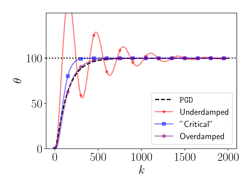
(a) Different regimes in MPD.

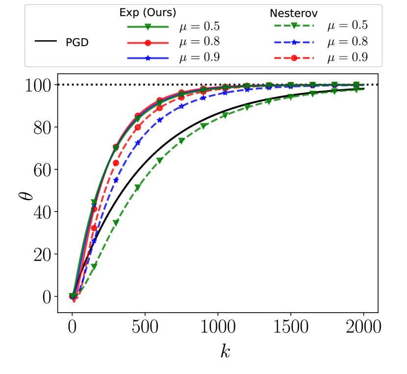
(b) $\theta_{t}$ integrator comparison.

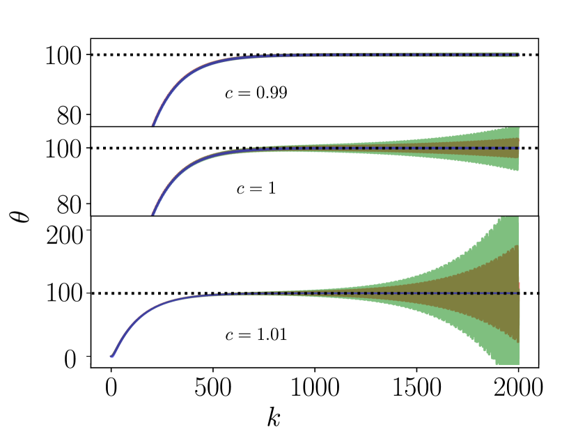
(c) Role of gradient correction.

Figure 1: Toy Hierarchical Model. (a) Different regimes that arise from varying the momentum parameters; (b) comparison between our Exponential (Exp) integrator and a Nesterov-like integrator for different momentum parameters; (c) we compare the performance of the MPD with and without gradient correction.

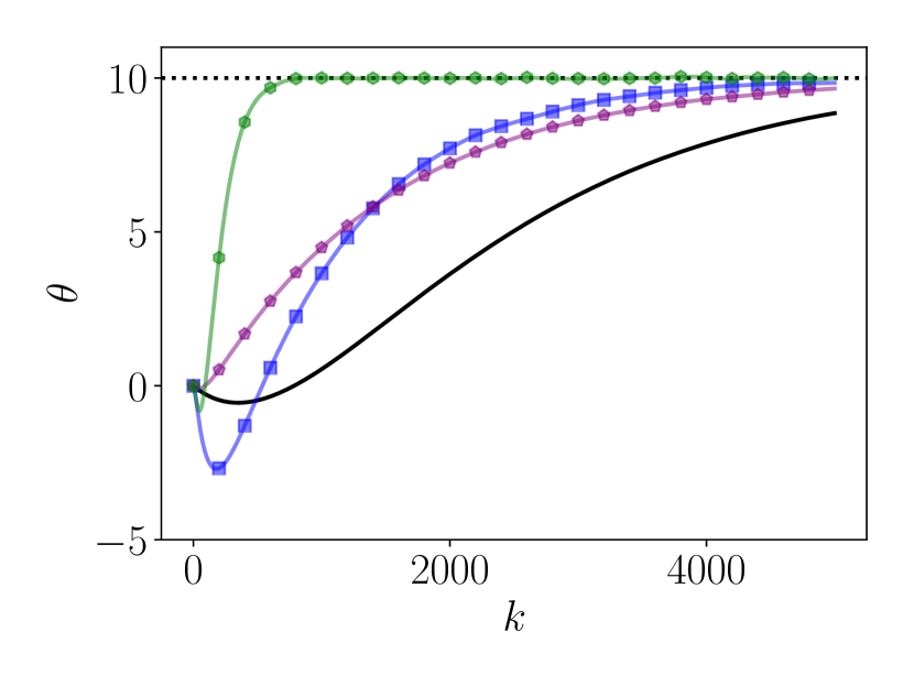
(a) $\mathcal{N}(-5,I)$.

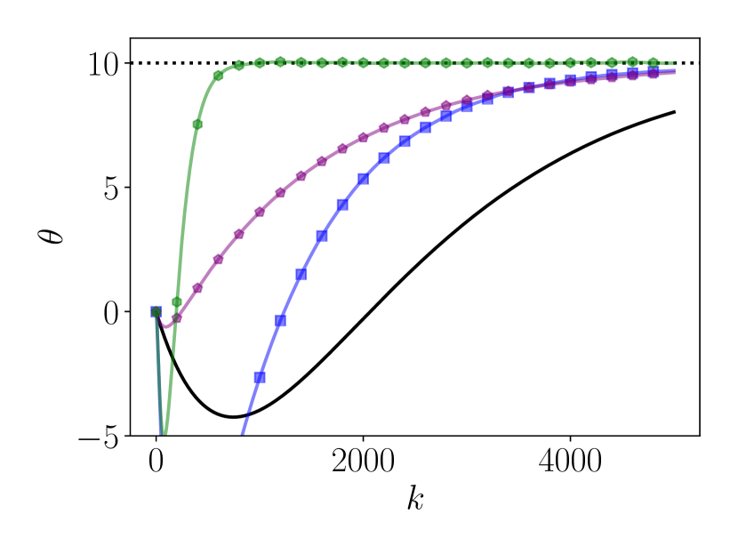
(b) $\mathcal{N}(-20,I)$.

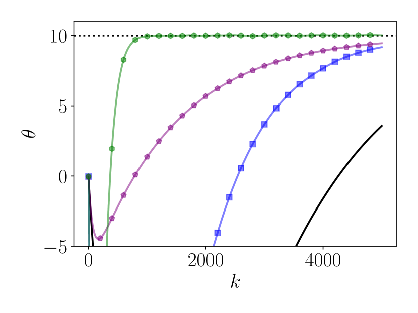
(c) $\mathcal{N}(-100,I)$.

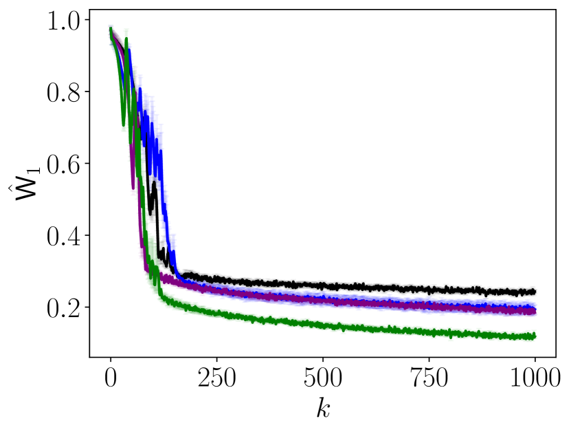
(d) $\hat{\mathsf{W}}_{1}$ distance vs iterations.

Figure 2: Comparison of MPD with algorithms that only enrich one component. (a), (b), (c) shows the performance on the $\mathrm{ToyHM}(10,12)$ with different initialization of the particle cloud $\{X_{0}^{i}\}_{i=1}^{M}$. In (d) shows the $\hat{\mathsf{W}}_{1}$ vs iterations of a density estimation problem on a Mixture of Gaussian dataset. MPD is shown in green, $\theta$-only-enriched shown in blue, $X$-only-enriched in purple, and PGD in black. The results are averaged over $10$ independent trials.

The astute reader will notice that our approximating ODE-SDE (i.e., Equation 21) deviates from Cheng et al., (2018)’s style of discretization. Specifically, the difference lies in where we compute the gradient in Equations 21b and 21d which we refer to as gradient correction. This subtle choice reflects the decision to utilize partially and fully updated approximations to $\tilde{\theta}_{h}$, i.e., the partially updated $\bar{\theta_{0}}$ in Equation 21b and fully updated $\tilde{\theta}_{h}$ in Equation 21d. This is reminiscent of NAG’s use of a partial parameter update to compute the gradient, unlike Polyak’s Heavy Ball, which does not (Sutskever et al., , 2013, Section 2.1). In our case, we empirically found that this choice is critical for a more stable discretization and enables the algorithm to be “faster” by taking larger step sizes (see Section 6.1).

The choice of the momentum parameters $\left(\eta_{\theta},\gamma_{\theta},\eta_{x},\gamma_{x}\right)$ is crucial to the practical performance of MPD. We observe that (as is also the case for NAG, the underdamped Langevin SDE, and other similar systems) there are three different qualitative regimes for the dynamics: i) the underdamped regime, in which the parameter values oscillate, ii) the overdamped regime, in which one recovers PGD-type behaviour, and iii) the critically-damped regime, in which oscillations are largely suppressed, but the momentum effects are still able to accelerate the convergence behaviour relative to PGD. While rigorous approaches are limited to simple targets (e.g., Dockhorn et al., (2022)), one can utilize cross-validation to obtain these parameters in practice.

6 Experiment

In this section, we study various design choices of MPD and demonstrate the efficacy of our proposal through empirical results. The structure of this section is as follows: in Section 6.1, we demonstrate on the Toy Hierarchical model the effects of various design choices; then, in Section 6.2, we compare MPD with algorithms that incorporate momentum in either $\theta$ or $X$ only; finally, in Section 6.3, we compare our proposal on training VAEs with other methods.

6.1 Toy Hierarchical Model

As a toy example, we consider the hierarchical model proposed in Kuntz et al., (2023). The model $\mathrm{ToyHM}(\theta,\sigma)$ is given by $p_{\theta}(y,x):=\prod_{i=1}^{N}\mathcal{N}(y_{i}|x_{i},1)\mathcal{N}(x_{i}|\theta,\sigma^{2})$, where $N=100$ is the number of data points. The dataset $y$ is sampled from a model with $\theta=100,\sigma=1$. In this experiment, we wish to understand the behaviour of MPD compared against PGD. We are particularly interested in (1) how the momentum parameters $\left(\eta_{\theta},\gamma_{\theta},\eta_{x},\gamma_{x}\right)$ affect the optimization process; (2) comparing our proposed discretization to another that follows in the style of NAG (detailed in Section I.3); and (3) the role of the gradient correction term described in Section 5. The results are shown in Figure 1. Further experiment details can be found in Section J.4.1.

In Figure 1(a), we show that different regimes can arise from different choices of hyper-parameters (as discussed in Section 3). In Figure 1(b), we compare the performance of MPD using (our) Exponential integrator with a NAG-like discretization for $(\theta_{t},m_{t})$-component. We vary the “momentum coefficient”, i.e., we have $\mu\in\{0.5,0.8,0.9\}$ with $\mu_{\theta}=\mu_{x}=\mu$. It can be seen that MPD with our exponential integrator for $\theta_{t}$ performs better than NAG-like integrator (see Section J.3 for more discussion). In Figure 1(c), we show the effect of the gradient correction term for three different step sizes in $(\theta,m)$-components while keeping the step sizes in $(X,U)$ fixed. The different lines in the figure are generated from a step size of $c\cdot 10^{-5/2}$ where $c\in\{0.99,1,1.01\}$. It can be seen that our proposed method is more effective than the other discretization. In red, we show MPD with the absence of gradient correction in Equation 21b (i.e., when we use $\theta_{0}$ instead of $\bar{\theta}_{0}$ in Equation 21b), and, in green, we show the MPD when the gradient correction is absent in both Equation 21b and Equation 21d (i.e. when we use $\theta_{0}$ instead of $\bar{\theta}_{0}$ and $\tilde{\theta}_{h}$ in Equation 21b and Equation 21d). It can be seen the gradient correction term results in a more stable algorithm.

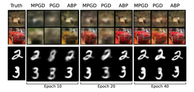
Figure 3: Posterior Cloud vs Epochs. We show the evolution of the reconstruction of a particle for persistent methods. The particle is taken at epoch $\{10,20,40\}$ on MNIST and CIFAR-10.

Dataset	MPD	PGD	ABP	SR	VI
MNIST	$\bm{47.9}\pm 0.6$	$104.1\pm 1.2$	$\bm{45.9}\pm 0.8$	$109.97\pm 12.5$	$72.6\pm 1.3$
CIFAR	$\bm{93.2}\pm 1.5$	$106.2\pm 4.8$	$97.0\pm 8.0$	$126.25\pm 13.0$	$\bm{94.2}\pm 6.7$

Table 1: FID scores on MNIST and CIFAR-10 after the final epoch. In bold, we indicate the lowest two scores on average. We write $(\mu\pm\sigma)$ to indicate the mean $\mu$ and standard deviation $\sigma$ of the FID score calculated over three independent trials.

6.2 Why Accelerate Both Components?

One may question the importance of momentum-enriching both components of PGD. We show in two experiments that enriching only one component results in a suboptimal algorithm. To show this, we consider the $\mathrm{ToyHM}(10,12)$, and, as a more realistic example, a $1$-d density estimation problem using a VAE on a Mixture of Gaussians with two equally weighted components which are $\mathcal{N}(2,0.5)$ and $\mathcal{N}(-2,0.5)$. To measure the performance of each algorithm, for the first problem, we examine the parameter of the model which should converge to the true value of $10$; and, for the second, we compute the empirical Wasserstein-1 $\hat{\mathsf{W}}_{1}$ using the empirical CDF.

Figure 2 shows the results of both experiments. Overall, it can be seen that the presence of momentum results in a better performance. Furthermore, we observe that the algorithms which only enrich one component can exhibit problems which are not present for MPD. For instance, in (a) (b) (c), poor initialization of the cloud drastically lengthens the transient phase of the $\theta$-only enriched algorithm, whereas MPD can recover more rapidly. This is a typical setting in high-dimensional settings (see (d)). Conversely, $X$-only-enriched algorithms are observed to suffer from slow convergence in the $\theta$-component (intuitively, one pays a larger price for poor conditioning of the ideal MLE objective). Overall, it can be observed that MPD noticeably outperforms PGD and all other intermediate methods in all settings. For details/discussion, see Appendix K.

6.3 Image Generation

For this task, we consider two datasets: MNIST (LeCun et al., , 1998) and CIFAR-10 (Krizhevsky and Hinton, , 2009). For the model, we use a variational autoencoder (Kingma and Welling, , 2014) with a VampPrior (Tomczak and Welling, , 2018). As baselines, we compare our proposed method MPD against PGD, Alternating Backpropagation (ABP) (Han et al., , 2017), Short Run (SR) (Nijkamp et al., , 2020), and amortized variational inference (VI) (Kingma and Welling, , 2014). ABP is the most similar to PGD. They differ in that ABP takes multiple steps of the (unadjusted and overdamped) Langevin algorithm (ULA) instead of PGD’s single step. They (MPD, PGD, ABP) are also persistent, meaning that the ULA chain starts at the previous particle location, whereas SR restarts the chain at a random location sampled from the prior but like ABP runs the chain for several steps. Further experiment details can be found in Section J.4.2.

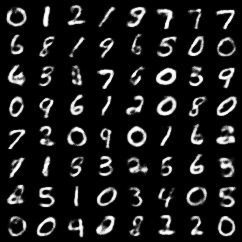
(a) MPD.

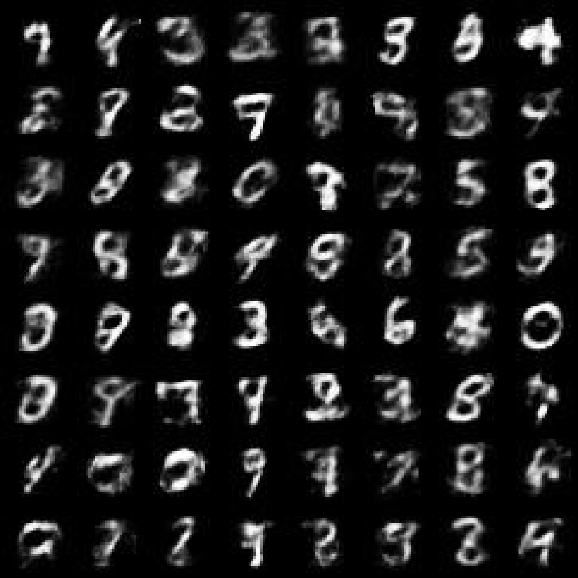
(b) PGD.

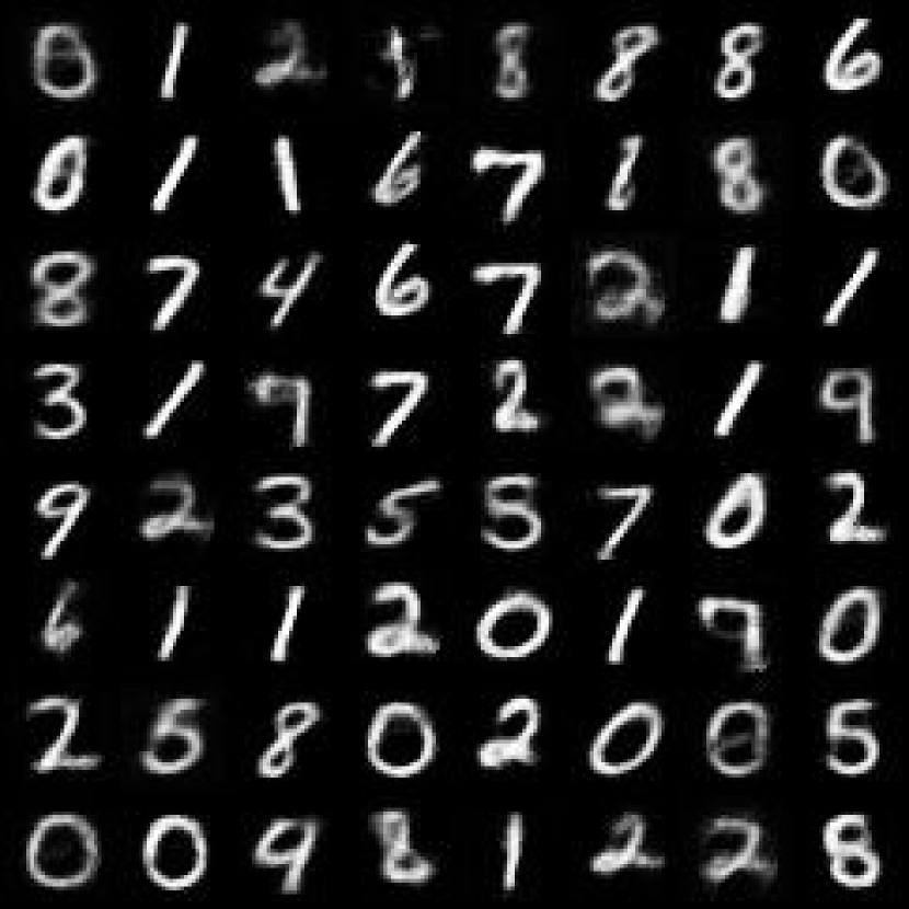
(c) VI.

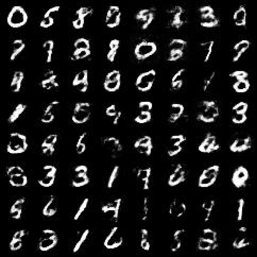
(d) ABP.

Figure 5: MNIST. Samples generated from various algorithms.

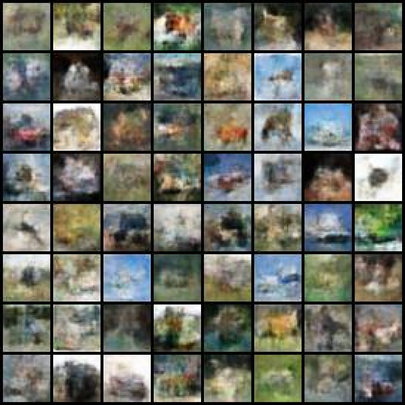
(a) MPD.

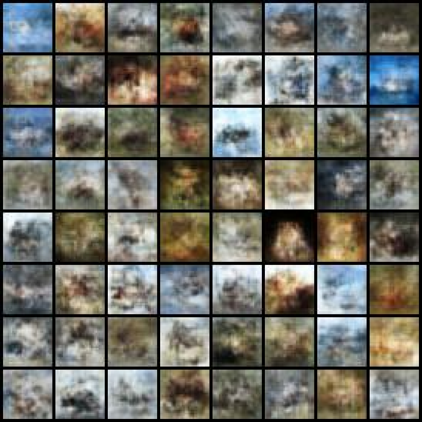
(b) PGD.

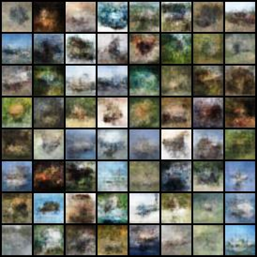
(c) VI.

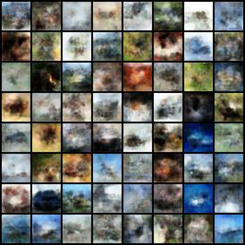
(d) ABP.

Figure 6: CIFAR-10. Samples generated from various algorithms.

We are interested in the generative performance of the resulting models. For a qualitative measure, we show the samples produced by the model in Figure 6 for CIFAR (for MNIST samples, see Figure 5 in the Appendix). As a quantitative measure, we report the Fréchet inception distance (FID) (Heusel et al., , 2017) as shown in Table 1. It can be seen that our proposed method does well compared against other baselines. The closest competitor is ABP. As noted by Kuntz et al., (2023), ABP can reap the benefits of taking multiple ULA steps to locate the posterior mode quickly and reduce the transient phase. This hypothesis is further confirmed in Figure 3, where we visualize the evolution of a single particle across various epochs. It can be seen that ABP’s and MPD’s distinct methods of reducing the transient phase (by taking multiple steps or utilizing momentum) are effective. As a competitor SR does perform badly, which we attribute to its non-persistent property: by restarting the particles at the prior and running short chains, it is unable to overcome the bias of short chains and locate the posterior mode. Variational inference performs well for CIFAR but surprisingly falls slightly short in MNIST.

7 Conclusion, Limitations, and Future work

We presented Momentum Particle Descent MPD, a method of incorporating momentum into particle gradient descent. We establish several theoretical results such as the convergence in continuous time; existence and uniqueness; as well as some guarantees for the usage of the particle approximation. Through experiments, we showed that, for suitably chosen momentum parameters, the resulting algorithm achieves better performance than PGD.

The main limitation that may impede the widespread adoption of MPD over PGD is the requirement for tuning the momentum parameters. This issue is inherited from the Underdamped Langevin dynamics where it is generally understood to be somewhat more challenging than its overdamped counterpart, as witnessed by the dearth of papers proposing practical tuning strategies for this class of algorithms. Although we found that the momentum coefficient heuristic (see Section J.3) worked well in our experiments, future work includes a systematic method of tuning momentum parameters $\left(\eta_{\theta},\gamma_{\theta},\eta_{x},\gamma_{x}\right)$ following Riou-Durand et al., (2023) (or some justification for using the momentum coefficient heuristic). Another future work is a theoretical characterization of the difference between our discretization scheme compared with other potential schemes akin to Sanz-Serna and Zygalakis, (2021).

[sections] [sections]l1

Appendix A Notation

The following table summarizes some key notation used throughout.

$\mathcal{E}$	Free Energy.
$\mathcal{F}$	Momentum-enriched Free Energy
$z_{t}$	The tuple $(\theta_{t},m_{t},q_{t})\in\mathbb{R}^{d_{\theta}}\times\mathbb{R}^{d_{\theta}}\times\mathcal{P}(\mathbb{R}^{d_{x}}\times\mathbb{R}^{d_{x}})$
$\nabla_{a}f$	Euclidean Gradient of $f$ w.r.t. $a$
$\nabla_{(a,b)}f$	$\left[\nabla_{a}f,\nabla_{b}f\right]^{\top}$
$\ell$	$\ell(\theta,x):=\log p_{\theta}(y,x)$
$\rho_{\theta}$	$\rho_{\theta}(x):=p_{\theta}(y,x)$
$\nabla_{a}\cdot$	Divergence operator w.r.t. $a$
$\nabla^{*}_{a}$	Adjoint operator of $\nabla_{a}$ (see Section F.4.2).
$[n]$	$[n]:=\{1,...,n\}$
$\Delta$	Laplacian operator, $\Delta=\nabla\cdot\nabla$
$\mathcal{P}(\mathbb{R}^{d})$	The space of probability measures that are absolutely continuous w.r.t. Lebesgue measure (have densities) and possess finite second moments.
$\left\langle{\cdot},{\cdot}\right\rangle$ (and $\|\cdot\|$)	Euclidean inner product or Frobenius inner product (and it’s inner norm)
$\left\langle{\cdot},{\cdot}\right\rangle_{\rho}$ (and $\|\cdot\|_{\rho}$)	$L^{2}(\rho)$ inner product (and its norm)
$o(\epsilon)$	Bachmann-Landau little-o notation
$\partial F(\mu)$	Fréchet subdifferential (see Definition C.1)

Appendix B Related Work

The present work sits at the juncture of i) deterministic gradient flows for optimising objectives over “parameter” spaces, typically expressible through the discretization of ODEs, and ii) stochastic gradient flows for optimising objectives over the space of probability measures, typically expressible through discretisation of mean-field SDEs. The former class of problems is too vast to be properly surveyed here (for an overview, see Santambrogio, (2017); Ambrosio et al., (2005)), effectively including a large proportion of modern continuous optimisation problems. The latter class has seen substantial growth over the past few years in particular, with various problems related to sampling (Liu, , 2017; Bernton, , 2018; Garbuno-Inigo et al., , 2020; Duncan et al., , 2023), variational inference (Yao and Yang, , 2022; Lambert et al., , 2022; Diao et al., , 2023), and the training of shallow neural networks (Mei et al., , 2018; Chizat and Bach, , 2018; Nitanda and Suzuki, , 2017; Hu et al., , 2021; Nitanda et al., , 2022; Chizat, , 2022; Chen et al., , 2022; Suzuki et al., , 2023) being studied in this framework. While there exist earlier works which combine optimisation with Markovian sampling (e.g. stochastic approximation approaches to the EM algorithm (Delyon et al., , 1999; De Bortoli et al., , 2021), training of energy-based models (Hinton, , 2002), and hyperparameter tuning in MCMC (Andrieu and Thoms, , 2008; Roberts and Rosenthal, , 2009)), the connection to gradient flows remains somewhat under-developed at present. We hope that the present work can encourage further exploration of these connections.

Appendix C Gradient Flow on $\mathbb{R}^{d_{\theta}}\times\mathcal{P}(\mathbb{R}^{d_{x}})$

In this section, we will describe gradient flows on the extended space $\mathbb{R}^{d_{\theta}}\times\mathcal{P}(\mathbb{R}^{d_{x}})$. We begin with an exposition of gradient flows in Wasserstein space, i.e. the space of distributions $\mathcal{P}(\mathbb{R}^{d_{x}})$ endowed with the Wasserstein-$2$ metric. We aim to give an intuitive introduction as opposed to a rigorous one; those readers with an interest in the latter are directed to Ambrosio et al., (2005). Using the ideas in Ambrosio et al., (2005), we show how the notion of gradients can be generalized to the product space $\mathbb{R}^{d_{\theta}}\times\mathcal{P}(\mathbb{R}^{d_{x}})$.

C.1 Gradient Flow on $\mathcal{P}(\mathbb{R}^{d_{x}})$

This exposition aims to introduce the intuition and necessary objects. We begin by describing the gradient flow on $\mathcal{P}(\mathbb{R}^{d_{x}})$ endowed with the Wasserstein-$2$ metric. The Wasserstein distance is defined as

$$\mathsf{W}_{2}^{2}(p,q)=\inf_{\pi\in\Pi(p,q)}\int_{\mathbb{R}^{d}\times\mathbb{R}^{d}}\left\|x-y\right\|^{2}\pi(\mathrm{d}x\times\mathrm{d}y),$$

where $\Pi(p,q)$ is the set of all couplings between $p$ and $q$.

In Ambrosio et al., (2005, Chapter 11), the authors discuss various approaches for adapting gradient flows on well-studied spaces (such as Euclidean and Riemannian spaces) to the Wasserstein space. One of these approaches proceeds by first defining suitable notions of tangent space and subdifferential, following which the simple definition of gradient flow modelled on Riemannian manifolds can then be reproduced. In this case, the Fréchet subdifferential (Ambrosio et al., , 2005, Definition 10.1.1) is defined as follow:

Definition C.1.

[Fréchet differential on Wasserstein Space] Let $F:\mathcal{P}(\mathbb{R}^{d_{x}})\rightarrow\mathbb{R}$ be a sufficiently regular function. We say that $\xi\in L^{2}(q)$ belongs to the Fréchet subdifferential $\partial F(q)$ if for all $q^{\prime}\in\mathcal{P}(\mathbb{R}^{d_{x}})$, we have

$$F(q^{\prime})-F(q)\geq\left\langle{\xi},{t_{q}^{q^{\prime}}-i}\right\rangle_{q}+o(\mathsf{W}_{2}(q,q^{\prime})),$$

where $t_{p}^{q}$ is the optimal map between $p$ and $q$ (Ambrosio et al., , 2005, see (7.1.4)) and $i$ is the identity map. Furthermore, if $\xi\in\partial F(q)$ also satisfies

$$F(t_{\#}q)-F(q)\geq\left\langle{\xi},{t-i}\right\rangle_{q}+o(\|t-i\|_{q}),$$

for all $t\in L^{2}(q)$, then we say that $\xi$ is a strong subdifferential.

See Ambrosio et al., (2005, Definition 10.1.1) for more details. The strong subdifferential can be thought of as the (Wasserstein) “gradient” of $F$. Equipped with this notion of gradient, we can define the gradient (descent) flow of $F:\mathcal{P}(\mathbb{R}^{d_{x}})\rightarrow\mathbb{R}$ as follows:

Definition C.2 (Gradient Flow).

We say that a curve $p_{t}:[0,1]\rightarrow\mathcal{P}(\mathbb{R}^{d_{x}})$ is a gradient flow of $F:\mathcal{P}(\mathbb{R}^{d_{x}})\rightarrow\mathbb{R}$ if for all $t>0$, it satisfies the continuity equation $\partial_{t}p_{t}+\nabla_{x}\cdot(v_{t}p_{t})=0$, where the tangent vector $v_{t}$ satisfies $-\,v_{t}\in\partial F(p_{t})$ for all $t$.

Thus, for our application, we are interested in computing the strong subdifferential of $F$. If $F$ is an integral of the type

$$F(p)=\int f(x,p(x),\nabla_{x}p(x))\mathrm{d}x,$$ (22)

where $f:\mathbb{R}^{d_{x}}\times\mathbb{R}\times\mathbb{R}^{d_{x}}\to\mathbb{R}$ is sufficiently regular, then we will see that its strong subdifferential admits an analytic solution.

Functionals of this form of great interest in the calculus of variations (e.g., see Gelfand and Silverman, (2000)). A vital quantity which is used to study these functionals is the first variation. Writing $\delta_{p}F[p]:\mathbb{R}^{d_{x}}\rightarrow\mathbb{R}$ for the first variation of $F$, the unique up to constants function such that

$$\left.\frac{\mathrm{d}}{\mathrm{d}\epsilon}F(q_{\epsilon})\right|_{\epsilon=0}=-\int\delta_{q}F[q](x)\,\nabla_{x}\cdot(q(x)v(x))\mathrm{d}x$$

for all $v$ such that $q_{\epsilon}:=(i+\epsilon v)_{\#}q\in\mathcal{P}(\mathbb{R}^{d_{x}})$ for sufficiently small $\epsilon$, one can readily establish that for (22)-typed $F$, it is given by

$$\delta_{p}F[p](x):=\nabla_{(2)}f(x,p(x),\nabla_{x}p(x))-\nabla_{x}\cdot(\nabla_{(3)}f(x,p(x),\nabla_{x}p(x)),$$

where $\nabla_{(i)}$ denotes the partial derivative w.r.t. the $i$-th argument (Ambrosio et al., , 2005, Eq. (10.4.2)). It can be shown that for any $\xi\in\partial F(p)$ which is a strong subdifferential, it holds that $\xi(x)\overset{p-a.e.}{=}\nabla_{x}\delta_{p}F[p](x)$ (Ambrosio et al., , 2005, Lemma 10.4.1).

C.2 Gradient flow on $\mathbb{R}^{d_{\theta}}\times\mathcal{P}(\mathbb{R}^{d_{x}})$

We provided here a generalization of the Fréchet differential (for a broad survey of Fréchet differentials, see Kruger, (2003)) to the extended space $\mathbb{R}^{d_{\theta}}\times\mathcal{P}(\mathbb{R}^{d_{x}})$:

Definition C.3 (Fréchet differential on $\mathbb{R}^{d_{\theta}}\times\mathcal{P}(\mathbb{R}^{d_{x}})$).

Let $\mathcal{F}:\mathbb{R}^{d_{\theta}}\times\mathcal{P}(\mathbb{R}^{d_{x}})\rightarrow\mathbb{R}$ be a sufficiently regular function. We say that $(\xi_{\theta},\xi_{q})\in\mathbb{R}^{d_{\theta}}\times L_{2}(q)$ belongs to the Fréchet subdifferential $\partial\mathcal{F}(\theta,q)$ if for all $(\theta^{\prime},q^{\prime})\in\mathbb{R}^{d_{\theta}}\times\mathcal{P}(\mathbb{R}^{d_{x}})$, it holds that

$$\mathcal{F}(\theta^{\prime},q^{\prime})-\mathcal{F}(\theta,q)\geq\left\langle{\xi_{\theta}},{\theta^{\prime}-\theta}\right\rangle+\left\langle{\xi_{q}},{t_{q}^{q^{\prime}}-i}\right\rangle_{q}+o(\mathsf{W}_{2}(q^{\prime},q)+\|\theta^{\prime}-\theta\|).$$

Furthermore, if $(\xi_{\theta},\xi_{q})\in\partial\mathcal{F}(\theta,q)$ also satisfies

$$\mathcal{F}(\theta+\tau,t_{\#}q)-\mathcal{F}(\theta,q)\geq\left\langle{\xi_{\theta}},{\tau}\right\rangle+\left\langle{\xi_{q}},{t-i}\right\rangle_{q}+o(\|t-i\|_{q}+\|\tau\|),$$

for all $(\tau,t)\in\mathbb{R}^{d_{\theta}}\times L_{2}(q)$, then we say that $(\xi_{\theta},\xi_{q})$ is a strong subdifferential.

For the remainder of the section, we shall assume that for any perturbation $(\sigma,v)$, there exists some $\delta_{q}F[\theta,q]:\mathbb{R}^{d_{x}}\rightarrow\mathbb{R}$ (often called the first variation) such that the following expansion holds:

$$\frac{\mathrm{d}}{\mathrm{d}\epsilon}\mathcal{F}(\theta_{\epsilon},q_{\epsilon})\big{|}_{\epsilon=0}= \left\langle{\nabla_{\theta}\mathcal{F}(\theta,q)},{\sigma}\right\rangle-\int\delta_{q}\mathcal{F}[\theta,q](x)\,\nabla_{x}\cdot(v(x)q(x))\,\mathrm{d}x,$$ (23)

where $q_{\epsilon}:=(i+\epsilon v)_{\#}q$ and $\theta_{\epsilon}:=\theta+\epsilon\sigma$. For all $\mathcal{F}$ of interest in this paper, this assumption holds; for instance, see Proposition F.4.

We follow in the argument of Ambrosio et al., (2005, Lemma 10.4.1) to show that if $(\xi_{\theta},\xi_{q})\in\partial\mathcal{F}(\theta,q)$ is a strong subdifferential, then we have that $\xi_{\theta}=\nabla_{\theta}\mathcal{F}(\theta,q)$ and $\xi_{q}(x)\overset{q-a.e.}{=}\nabla_{x}\delta_{q}\mathcal{F}[\theta,q](x)$. Let $(\xi_{\theta},\xi_{p})\in\partial\mathcal{F}(\theta,p)$ be a strong subdifferential. By using the strong subdifferential property for some perturbation $(\epsilon\sigma,\epsilon v)$ and taking left and right limits of (C.3), we obtain that

$$\limsup_{\epsilon\uparrow 0}\frac{\mathcal{F}(\theta_{\epsilon},q_{\epsilon})-\mathcal{F}(\theta,q)}{\epsilon}\leq\left\langle{\xi_{\theta}},{\sigma}\right\rangle+\left\langle{\xi_{q}},{v}\right\rangle_{q}\leq\liminf_{\epsilon\downarrow 0}\frac{\mathcal{F}(\theta_{\epsilon},q_{\epsilon})-\mathcal{F}(\theta,q)}{\epsilon}.$$

On the other hand, from our assumption (23), we have that

$$\lim_{\epsilon\rightarrow 0}\frac{\mathcal{F}(\theta_{\epsilon},q_{\epsilon})-\mathcal{F}(\theta,q)}{\epsilon} =\left\langle{\nabla_{\theta}\mathcal{F}(\theta,q)},{\sigma}\right\rangle-\int\delta_{q}\mathcal{F}[\theta,q](x)\,\nabla_{x}\cdot(v(x)q(x))\,\mathrm{d}x$$

$$=\left\langle{\nabla_{\theta}\mathcal{F}(\theta,q)},{\sigma}\right\rangle+\left\langle{\nabla_{x}\delta_{q}\mathcal{F}[\theta,q]},{v}\right\rangle_{q},$$

where the last equality follows from integration by parts and the divergence theorem. Hence, we have that $\xi_{\theta}=\nabla_{\theta}\mathcal{F}(\theta,q)$, and $\xi_{q}\overset{q-a.e.}{=}\nabla_{x}\delta_{q}\mathcal{F}[\theta,q]$.

C.3 First Variation

In this section, we derive the first variation for integral expressions taking a certain form. In particular, we are interested in computing the strong subdifferential of $\mathcal{F}$ of the following types:

$$\mathcal{F}(\theta,q) :=\int{f}(\theta,x,q(x),\nabla_{x}q(x))\mathrm{d}x,$$ (VI-I)

$$\mathcal{F}(\theta,q) :=\int\int f(\theta,x,y,q(x),q(y))\mathrm{d}x\mathrm{d}y.$$ (VI-II)

An exampled of (VI-I)-typed $\mathcal{F}$ is when $\mathcal{F}$ is the free energy $\mathcal{E}$. Following standard techniques from the calculus of variations (Gelfand and Silverman, , 2000), consider a perturbation $(\sigma,v)\in\mathbb{R}^{d_{\theta}}\times L_{2}(q)$ and define a mapping $\Phi$ by

$$\Phi(\epsilon):=\mathcal{F}(\theta_{\epsilon},q_{\epsilon}),$$

where $q_{\epsilon}:=(i+\epsilon v)_{\#}q$ and $\theta_{\epsilon}:=\theta+\epsilon\sigma$.

(VI-I)-typed $\mathcal{F}$. By application of the change-of-variables formula (for instance, see Ambrosio et al., (2005, Lemma 5.5.3)), we can compute the density $q_{\epsilon}$ and its derivative $\frac{\partial}{\partial\epsilon}q_{\epsilon}(y)$ as follows:

$$q_{\epsilon}(y) =\frac{q}{\mathrm{det}(I+\epsilon\nabla_{x}v)}\circ(i+\epsilon v)^{-1}(y),\quad\frac{\partial}{\partial\epsilon}q_{\epsilon}(y)\big{|}_{\epsilon=0}=-\nabla_{x}\cdot[qv](y).$$

Thus, we can compute the derivative of $\Phi$, provided that the interchange of derivative and integral can be justified, as

$$\frac{\mathrm{d}}{\mathrm{d}\epsilon}\Phi(\epsilon)\bigg{|}_{\epsilon=0}= \int\frac{\mathrm{d}}{\mathrm{d}\epsilon}f(\theta_{\epsilon},x,q_{\epsilon}(x),\nabla_{x}q_{\epsilon}(x))\,\mathrm{d}x$$

$$= \int\left\langle{\nabla_{\theta}f(\theta,x,q(x),\nabla_{x}q(x))},{\sigma}\right\rangle\,\mathrm{d}x$$

$$-\int\nabla_{(3)}f(\theta,x,q(x),\nabla_{x}q(x))\,\nabla_{x}\cdot[vq](x)\,\mathrm{d}x$$

$$-\int\left\langle{\nabla_{(4)}f(\theta,x,q(x),\nabla_{x}q(x))},{\nabla_{x}[\nabla_{x}\cdot[vq]](x)}\right\rangle\,\mathrm{d}x$$

Applying integration by parts and the divergence theorem, we obtain that

$$\frac{\mathrm{d}}{\mathrm{d}\epsilon}\Phi(\epsilon)\bigg{|}_{\epsilon=0}= \left\langle{\nabla_{\theta}\mathcal{F}(\theta,q)},{\sigma}\right\rangle$$

$$-\int\nabla_{(3)}f(\theta,x,q(x),\nabla_{x}q(x))\,[\nabla_{x}\cdot(vq)](x)\,\mathrm{d}x$$

$$+\int\nabla_{x}\cdot[\nabla_{(4)}f](\theta,x,q(x),\nabla_{x}q(x))[\nabla_{x}\cdot(vq)](x)\,\mathrm{d}x$$

We can hence write the first variation of (VI-I)-typed $\mathcal{F}$ as

$$\delta_{q}\mathcal{F}[\theta,q](x)=\nabla_{(3)}f(\theta,x,q(x),\nabla_{x}q(x))-\nabla_{x}\cdot(\nabla_{(4)}f(\theta,x,q(x),\nabla_{x}q(x)).$$ (24)

(VI-II)-typed $\mathcal{F}$. Similarly to above, we can define $\Phi(\epsilon):=\mathcal{F}(\theta_{\epsilon},q_{\epsilon})$, whose derivative is given by

$$\frac{\mathrm{d}}{\mathrm{d}\epsilon}\Phi(\epsilon)\bigg{|}_{\epsilon=0}= \left\langle{\nabla_{\theta}\mathcal{F}(\theta,q)},{\sigma}\right\rangle$$

$$-\int\int\nabla_{(4)}f(\theta,x,y,q(x),q(y))\,\nabla_{x}\cdot[qv](x)\,\mathrm{d}x\,\mathrm{d}y$$

$$-\int\int\nabla_{(5)}f(\theta,x,y,q(x),q(y))\,\nabla_{y}\cdot[qv](y)\,\mathrm{d}x\,\mathrm{d}y.$$

Hence, the first variation is given by

$$\delta_{q}\mathcal{F}[\theta,q](x)= \int\left[\nabla_{(4)}f(\theta,x,y,q(x),q(y))+\nabla_{(5)}f(\theta,y,x,q(y),q(x))\right]\mathrm{d}y.$$ (25)

Example 1 (First Variation of $\mathcal{E}$).

It can be seen that the free energy is (VI-I)-typed with $f(\theta,x,a,g)=a\cdot\log\frac{a}{p_{\theta}(y,x)}$. Hence, by combining the formula (24) with the fact that

$$\nabla_{3}f(\theta,x,a,b) =\log\frac{a}{p_{\theta}}+1,$$

$$\nabla_{4}(f(\theta,x,a,g) =0,$$

we obtain the following expression for the first variation:

$$\delta_{q}\mathcal{F}[\theta,q](x)=\log\frac{q(x)}{p_{\theta}(y,x)}+1.$$

This provides an alternative derivation of this expression to that given in Kuntz et al., (2023, Lemma 1).

Appendix D A log Sobolev inequality for $\mathcal{E}$ can be transferred to $\mathcal{F}$

In this section, we show that nice properties of the functional $\mathcal{E}$ transfer to the functional $\mathcal{F}$, i.e. if $\mathcal{E}$ satisfies a log Sobolev inequality (2), then so does $\mathcal{F}$ (with a modified constant):

Proposition D.1.

If 2 holds, then upon defining $C:=\min\{C_{\mathcal{E}},\eta_{\theta},\eta_{x}\}$, it holds that

$$\mathcal{F}(\theta,m,q)-\mathcal{E}^{*}\leq\frac{1}{2C}\left|\left|{\nabla\mathcal{F}(\theta,m,q)}\right|\right|_{q}^{2},\quad\forall\theta,m\in\mathbb{R}^{d_{\theta}},\enskip q\in\mathcal{P}(\mathbb{R}^{2d_{x}}),$$

where

$$\left|\left|{\nabla\mathcal{F}(\theta,m,q)}\right|\right|_{q}^{2}:=\|\nabla_{(\theta,m)}\mathcal{F}(\theta,m,q)\|^{2}+\|\nabla_{(x,u)}\log q-\nabla_{(x,u)}\log\rho_{\theta,\eta_{x}}\|^{2}_{q}.$$ (26)

Proof.

As we show at the end of the proof, we have the fact that

$$\left|\left|{\nabla_{(x,u)}\log\left(\frac{q}{\rho_{\theta}\otimes r_{\eta_{x}}}\right)}\right|\right|_{q}^{2}\geq{\left|\left|{\nabla_{x}\log\left(\frac{q_{X}}{\rho_{\theta}}\right)}\right|\right|^{2}}_{q(\mathrm{d}x)}+{\left|\left|{\nabla_{u}\log\frac{q_{U|X}}{r_{\eta_{x}}}}\right|\right|^{2}}_{q}.$$ (27)

From the definition, we have

$$\left|\left|{\nabla\mathcal{F}(\theta,m,q)}\right|\right|_{q}^{2}=\left|\left|{\nabla_{\theta}\mathcal{F}(\theta,m,q)}\right|\right|^{2}+\left|\left|{\eta_{\theta}m}\right|\right|^{2}+\left|\left|{\nabla_{(x,u)}\log\frac{q}{\rho_{\theta,\eta_{x}}}}\right|\right|_{q}^{2}.$$

Using  (27) and the fact that

$$\nabla_{\theta}\mathcal{F}(\theta,m,q)=-\int\nabla_{\theta}\log p_{\theta}(y,x,u)q(\mathrm{d}x,\mathrm{d}u)=-\int\nabla_{\theta}\log p_{\theta}(y,x)q(\mathrm{d}x)=\nabla_{\theta}\mathcal{E}(\theta,q),$$

then it follows that

$$\left|\left|{\nabla\mathcal{F}(\theta,m,q)}\right|\right|_{q}^{2}\geq \left|\left|{\nabla_{\theta}\mathcal{E}(\theta,q_{X})}\right|\right|_{q}^{2}+\eta_{\theta}^{2}\left|\left|{m}\right|\right|^{2}+{\left|\left|{\nabla_{u}\log\frac{q_{U|X}}{r_{\eta}}}\right|\right|^{2}}_{q}.$$

Because $C=\min\{C_{\mathcal{E}},\eta_{\theta},\eta_{x}\}$, the above implies that

$$\frac{1}{2C}\left|\left|{\nabla\mathcal{F}(\theta,m,q)}\right|\right|_{q}^{2} \geq\frac{1}{2C_{\mathcal{E}}}\left|\left|{\nabla_{\theta}\mathcal{E}(\theta,q)}\right|\right|_{q}^{2}+\frac{\eta_{\theta}}{2}\left|\left|{m}\right|\right|^{2}+\frac{1}{2\eta_{x}}{\left|\left|{\nabla_{u}\log\frac{q_{U|X}}{r_{\eta_{x}}}}\right|\right|^{2}_{q}}.$$ (28)

Since $r_{\eta_{x}}=\mathcal{N}(0,\eta_{x}^{-1}I_{d_{x}})$ is $\eta_{x}$-strongly log-concave, by the Bakry-Émery criterion of Bakry and Émery, (2006), it holds that

$$\frac{1}{2\eta_{x}}{\left|\left|{\nabla_{u}\log\left(\frac{q(\cdot|x)}{r_{\eta_{x}}}\right)}\right|\right|^{2}_{q(\mathrm{d}u|x)}}\geq\mathsf{KL}(q_{U|x}|r_{\eta_{x}})\quad\forall x\in\mathcal{X},$$

and so we obtain that

$$\frac{1}{2\eta_{x}}{\left|\left|{\nabla_{u}\log\frac{q_{U|X}}{r_{\eta_{x}}}}\right|\right|^{2}}_{q} =\frac{1}{2\eta_{x}}\mathbb{E}_{q_{X}}\left[\left|\left|{\nabla_{u}\log\frac{q(\cdot|X)}{r_{\eta_{x}}}}\right|\right|^{2}_{q(du|\cdot)}\right]$$

$$\geq\mathbb{E}_{q(\mathrm{d}x)}\left[\mathsf{KL}(q_{U|x}|r_{\eta_{x}})\right].$$

Plugging the above into (28) and using the log Sobolev inequality for $\mathcal{E}$, we obtain that for $\mathcal{F}$:

$$\frac{1}{2C}\left|\left|{\nabla\mathcal{F}(\theta,m,q)}\right|\right|_{q}^{2} \geq\mathcal{E}(\theta,q_{X})-\mathcal{E}^{*}+\frac{\eta_{\theta}}{2}\|m\|_{2}^{2}+\mathbb{E}_{q(\mathrm{d}x)}\left[\mathsf{KL}(q_{U|X}|r_{\eta_{x}})\right]$$

$$\geq\mathcal{F}(\theta,m,q)-\mathcal{E}^{*}.$$

We have one loose end to tie up: proving (27). To do so, note that

$$\left|\left|{\nabla_{(x,u)}\log\left(\frac{q}{\rho_{\theta}\otimes r_{\eta_{x}}}\right)}\right|\right|_{q}^{2}= {\left|\left|{\nabla_{(x,u)}\log\left(\frac{q_{X}}{\rho_{\theta}}\right)+\nabla_{(x,u)}\log\left(\frac{q_{U|X}}{r_{\eta_{x}}}\right)}\right|\right|^{2}_{q}}$$

$$= {\left|\left|{\nabla_{x}\log\left(\frac{q_{X}}{\rho_{\theta}}\right)+\nabla_{x}\log q_{U|X}}\right|\right|^{2}_{q}}$$ (29)

$$+{\left|\left|{\nabla_{u}\log\left(\frac{q_{U|X}}{r_{\eta_{x}}}\right)}\right|\right|^{2}_{q}}.$$ (30)

Taking the first term and expanding the square, we have

$$\left|\left|{\nabla_{x}\log\left(\frac{q_{X}}{\rho_{\theta}}\right)+\nabla_{x}\log q_{U|X}}\right|\right|^{2}_{q}= {\left|\left|{\nabla_{x}\log\left(\frac{q_{X}}{\rho_{\theta}}\right)}\right|\right|^{2}_{q}}$$

$$+2\left\langle{\nabla_{x}\log\left(\frac{q_{X}}{\rho_{\theta}}\right)},{\nabla_{x}\log q_{U|X}}\right\rangle_{q}$$

$$+{\left|\left|{\nabla_{x}\log q_{U|X}}\right|\right|^{2}_{q}}.$$

Applying Jensen’s inequality to the final term, we obtain

$$\left|\left|{\nabla_{x}\log\left(\frac{q_{X}}{\rho_{\theta}}\right)+\nabla_{x}\log q_{U|X}}\right|\right|^{2}_{q}\geq {\left|\left|{\nabla_{x}\log\left(\frac{q_{X}}{\rho_{\theta}}\right)}\right|\right|^{2}}_{q(\mathrm{d}x)}$$

$$+2{\left\langle{\nabla_{x}\log\left(\frac{q_{X}}{\rho_{\theta}}\right)},{\mathbb{E}_{q(\mathrm{d}u|\cdot)}\left[\nabla_{x}\log q(U|\cdot)\right]}\right\rangle_{q(\mathrm{d}x)}}$$

$$+{\left|\left|{\mathbb{E}_{q(\mathrm{d}u|\cdot)}\left[\nabla_{x}\log q(U|\cdot)\right]}\right|\right|^{2}_{q(\mathrm{d}x)}}.$$

One can compute explicitly that for all $x$, it holds that $\mathbb{E}_{q(\mathrm{d}u|x)}\left[\nabla_{x}\log q(U|x)\right]=0$; we thus obtain that

$$\left|\left|{\nabla_{x}\log\frac{q_{X}}{\rho_{\theta}}+\nabla_{x}\log q_{U|X}}\right|\right|^{2}_{q}\geq\left|\left|{\nabla_{x}\log\frac{q_{X}}{\rho_{\theta}}}\right|\right|^{2}_{q(\mathrm{d}x)},$$

and so (27) follows from (30). ∎

Appendix E $\mathcal{F}(z_{t})$ is non-increasing

In the following proposition, we show that $\mathcal{F}_{t}:=\mathcal{F}(z_{t})$ is non-increasing in time.

Proposition E.1.

For any $\gamma_{x}\geq 0$ and $\gamma_{\theta}\geq 0$, it holds that

$$\dot{\mathcal{F}}_{t}=-\gamma_{\theta}\|\nabla_{m}\mathcal{F}_{t}\|^{2}-\gamma_{x}\|\nabla_{u}\delta_{q}\mathcal{F}_{t}\|^{2}_{q_{t}}\leq 0.$$

Proof.

We begin by computing the time derivative

$$\dot{\mathcal{F}}_{t}= -\left\langle\nabla_{(\theta,m)}\mathcal{F}_{t},\begin{pmatrix}0&-I_{d_{\theta}}\\ I_{d_{\theta}}&\gamma_{\theta}I_{d_{\theta}}\end{pmatrix}\nabla_{(\theta,m)}\mathcal{F}_{t}\right\rangle$$ (31)

$$-\left\langle\nabla_{(x,u)}\delta_{q}\mathcal{F}_{t},\begin{pmatrix}0&-I_{d_{x}}\\ I_{d_{x}}&\gamma_{x}I_{d_{x}}\end{pmatrix}\nabla_{(x,u)}\delta_{q}\mathcal{F}_{t}\right\rangle_{q_{t}}.$$ (32)

Decomposing the matrix $\begin{pmatrix}0&-I_{d_{\theta}}\\ I_{d_{\theta}}&\gamma_{\theta}I_{d_{\theta}}\end{pmatrix}$ into symmetric and skew-symmetric components (write $D$, $Q$ respectively), i.e.

$$\begin{pmatrix}0&-I_{d_{\theta}}\\ I_{d_{\theta}}&\gamma_{\theta}I_{d_{\theta}}\end{pmatrix}=\underbrace{\begin{pmatrix}0&-I_{d_{\theta}}\\ I_{d_{\theta}}&0\end{pmatrix}}_{=:Q}+\underbrace{\begin{pmatrix}0&0\\ 0&\gamma_{\theta}I_{d_{\theta}}\end{pmatrix}}_{=:D},$$

we can simplify the RHS of (31) to

$$\text{RHS }\eqref{eq:dFdt_t1}=-\left\langle\nabla_{(\theta,m)}\mathcal{F}_{t},D\nabla_{(\theta,m)}\mathcal{F}_{t}\right\rangle=-\gamma_{\theta}\|\nabla_{m}\mathcal{F}_{t}\|^{2}.$$

Similarly, we can show that

$$\eqref{eq:dFdt_t2}=-\gamma_{x}\|\nabla_{u}\delta_{q}\mathcal{F}_{t}\|^{2}_{q_{t}}.$$

As such, for $\gamma_{x}\geq 0$, $\gamma_{\theta}\geq 0$, the claim follows. ∎

Appendix F Proof of Theorem 4.1

The outline of the proof of Theorem 4.1 is:

• Step 1 (Section F.1): Explicitly computing an upper bound of the time derivative of $\mathcal{F}$ as a quadratic form.

• Step 2 (Section F.2): Under the conditions specified in (50), we show that this time derivative is bounded above by another quadratic form that allows us to apply the log Sobolev inequality of Proposition D.1.

• Step 3: Using log Sobolev inequality, Proposition D.1, and Grönwall’s inequality, we obtain the desired result.

The remainder of the sections are dedicated to supporting the proof of Steps 1 and 2. This is done by developing the technical tools and carrying out explicit computations. The particular roles of the following sections are:

1. Section F.4.1: Computing the time derivative of $\mathcal{L}$ for Step 1.

2. Sections F.4.3, F.4.2 and F.4.4: Introducing the adjoint, commutator and another operator, as well as their explicit forms.

3. Section F.4.5: Using the operators and explicit forms in Sections F.4.3, F.4.2 and F.4.4, we can upper bound terms introduced in Section F.4.1 for Step 1. We utilize this in Step 1.

4. Section F.4.6. Bounding the cross terms (or interaction terms) between $\theta$ and $x$ that arises in the time derivative.

5. Section F.4.7. Establishing sufficient conditions for a matrix with a particular form to be positive semi-definite given in Proposition F.18. This is used in Step 2.

Recall that the Lyapunov function is given by:

$$\mathcal{L}:=\mathcal{F}-\mathcal{E}^{*}+\left\|\nabla_{\left(\theta,m\right)}\mathcal{F}\right\|_{T_{\left(\theta,m\right)}}^{2}+\left\|\nabla_{\left(x,u\right)}\delta_{q}\mathcal{F}\right\|_{T_{\left(x,u\right)}}^{2}$$

where

$$T_{(\theta,m)}:=\frac{1}{K}\begin{pmatrix}\tau_{\theta}I_{d_{\theta}}&\frac{\tau_{\theta m}}{2}I_{d_{\theta}}\\ \frac{\tau_{\theta m}}{2}I_{d_{\theta}}&\tau_{m}I_{d_{\theta}}\end{pmatrix},\quad T_{(x,u)}:=\frac{1}{K}\begin{pmatrix}\tau_{x}I_{d_{x}}&\frac{\tau_{xu}}{2}I_{d_{x}}\\ \frac{\tau_{xu}}{2}I_{d_{x}}&\tau_{u}I_{d_{x}}\end{pmatrix}$$ (33)

Proof of Theorem 4.1.

The proof is completed in the following three steps:

Step 1. In Section F.1, we show that the time derivative of $\mathcal{L}(z_{t})$ satisfies the following upper bound:

$$\frac{\mathrm{d}}{\mathrm{d}t}\mathcal{L}_{t}\leq -\left\langle{\nabla_{(\theta,m)}\mathcal{F}_{t}},{S_{(\theta,m)}\nabla_{(\theta,m)}\mathcal{F}_{t}}\right\rangle-\left\langle{\nabla_{(x,u)}\delta_{q}\mathcal{F}_{t}},{S_{(x,u)}\nabla_{(x,u)}\delta_{q}\mathcal{F}_{t}}\right\rangle_{q_{t}}.$$

where $S_{(x,u)}$ and $S_{(\theta,m)}$ are suitable matrices defined in (46) and (47), respectively.

Step 2. Then, in Section F.2, when Equation 50 holds for some rate $\varphi>0$, we have that

$$S_{(\theta,m)} \succeq\varphi C\left(T_{(\theta,m)}+\frac{1}{2C}I_{d_{\theta}}\right),$$

$$S_{(x,u)} \succeq\varphi C\left(T_{(x,u)}+\frac{1}{2C}I_{d_{x}}\right),$$

where $C:=\min\{C_{\mathcal{E}},\eta_{\theta},\eta_{x}\}$.

Step 3. By Step $1$ and Step $2$, we obtain

$$\frac{\mathrm{d}}{\mathrm{d}t}\mathcal{L}_{t}\leq -\varphi C\left(\frac{1}{2C}\left|\left|{\nabla_{(\theta,m)}\mathcal{F}_{t}}\right|\right|^{2}+\left\|\nabla_{\left(\theta,m\right)}\mathcal{F}_{t}\right\|_{T_{\left(\theta,m\right)}}^{2}\right)$$

$$-\varphi C\left(\frac{1}{2C}{\left|\left|{\nabla_{(x,u)}\delta_{q}\mathcal{F}_{t}}\right|\right|^{2}_{q_{t}}}+\left\|\nabla_{\left(x,u\right)}\delta_{q}\mathcal{F}_{t}\right\|_{T_{\left(x,u\right)}}^{2}\right).$$

Comparing the above to (26), applying Proposition D.1 and the Equation 18,

$$\frac{\mathrm{d}}{\mathrm{d}t}\mathcal{L}_{t}\leq-\varphi C\mathcal{L}_{t},$$

and application of Gronwall’s inequality yields the final result

$$\mathcal{F}_{t}-\mathcal{E}^{*}\leq\mathcal{L}_{0}\exp\left(-\varphi Ct\right).$$

∎

F.1 Proof of Step 1

As shown in Proposition F.2, the time derivative of the Lyapunov function $\mathcal{L}$ is given by

$$\frac{\mathrm{d}}{\mathrm{d}t}\mathcal{L}_{t}= -\left\langle{\nabla_{(\theta,m)}\mathcal{L}_{t}},{\begin{pmatrix}0&-I_{d_{\theta}}\\ I_{d_{\theta}}&\gamma_{\theta}I_{d_{\theta}}\end{pmatrix}\nabla_{(\theta,m)}\mathcal{F}_{t}}\right\rangle$$ (34)

$$-\left\langle{\nabla_{(x,u)}\delta_{q}\mathcal{L}_{t}},{\begin{pmatrix}0&-I_{d_{x}}\\ I_{d_{x}}&\gamma_{\theta}I_{d_{x}}\end{pmatrix}\nabla_{(x,u)}\delta_{q}\mathcal{F}_{t}}\right\rangle_{q_{t}},$$ (35)

where we abbreviate $\mathcal{L}_{t}:=\mathcal{L}(z_{t})$ and $\mathcal{F}_{t}:=\mathcal{F}(z_{t})$.

We deal with the inner products in (34,35) one-by-one, starting with (34): we first compute the gradient of $\mathcal{L}$ w.r.t. to $(\theta,m)$, finding that

$$\nabla_{\left(\theta,m\right)}\mathcal{L}=\nabla_{(\theta,m)}\mathcal{F}+2[\nabla_{(\theta,m)}^{2}\mathcal{F}]\,T_{(\theta,m)}\nabla_{(\theta,m)}\mathcal{F}+2\mathbb{E}_{q}\left[[\nabla_{(\theta,m)}\nabla_{(x,u)}\delta_{q}\mathcal{F}]\,T_{(x,u)}\nabla_{(x,u)}\delta_{q}\mathcal{F}\right],$$

where, as before, assume that the derivative-integral exchange can justified (see Section C.3). It then follows that

$$\eqref{eq:dldthetadt} =-\left\langle{\nabla_{(\theta,m)}\mathcal{F}_{t}},{\tilde{\Gamma}_{\theta}\nabla_{(\theta,m)}\mathcal{F}_{t}}\right\rangle$$ (36)

$$-2\left\langle{\nabla_{(\theta,m)}\nabla_{(x,u)}[\delta_{q}\mathcal{F}_{t}]\,T_{(x,u)}\nabla_{(x,u)}\delta_{q}\mathcal{F}_{t}},{\begin{pmatrix}0&-I_{d_{\theta}}\\ I_{d_{\theta}}&\gamma_{\theta}I_{d_{\theta}}\end{pmatrix}\nabla_{(\theta,m)}\mathcal{F}_{t}}\right\rangle_{q_{t}}.$$ (37)

where

$$\tilde{\Gamma}_{\theta}:=\begin{pmatrix}0&-I_{d_{\theta}}\\ I_{d_{\theta}}&\gamma_{\theta}I_{d_{\theta}}\end{pmatrix}+2T_{(\theta,m)}\nabla_{(\theta,m)}^{2}\mathcal{F}_{t}\begin{pmatrix}0&-I_{d_{\theta}}\\ I_{d_{\theta}}&\gamma_{\theta}I_{d_{\theta}}\end{pmatrix}.$$

By $\mathcal{F}$’s definition,

$$\nabla^{2}_{(\theta,m)}\mathcal{F}=\begin{pmatrix}\nabla^{2}_{\theta}\mathcal{F}&0_{d_{\theta}}\\ 0_{d_{\theta}}&\eta_{\theta}I_{d_{\theta}}\end{pmatrix};$$

whence we see that

$$\nabla_{(\theta,m)}^{2}\mathcal{F}\begin{pmatrix}0_{d_{\theta}}&-I_{d_{\theta}}\\ I_{d_{\theta}}&\gamma_{\theta}I_{d_{\theta}}\end{pmatrix} =\begin{pmatrix}0_{d_{\theta}}&-\nabla_{\theta}^{2}\mathcal{F}\\ \eta_{\theta}I_{d_{\theta}}&\gamma_{\theta}\eta_{\theta}I_{d_{\theta}}\end{pmatrix}$$

$$\Rightarrow T_{(\theta,m)}\nabla_{(\theta,m)}^{2}\mathcal{F}\begin{pmatrix}0_{d_{\theta}}&-I_{d_{\theta}}\\ I_{d_{\theta}}&\gamma_{\theta}I_{d_{\theta}}\end{pmatrix} =\begin{pmatrix}\frac{\tau_{\theta m}\eta_{\theta}}{2}I_{d_{\theta}}&\frac{\tau_{\theta m}\gamma_{\theta}\eta_{\theta}}{2}I_{d_{\theta}}-\tau_{\theta}\nabla_{\theta}^{2}\mathcal{F}\\ \tau_{m}\eta_{\theta}I_{d_{\theta}}&\tau_{m}\gamma_{\theta}\eta_{\theta}I_{d_{\theta}}-\frac{\tau_{\theta m}}{2}\nabla_{\theta}^{2}\mathcal{F}\end{pmatrix},$$

$$\Rightarrow\tilde{\Gamma}_{\theta} =\begin{pmatrix}\tau_{\theta m}\eta_{\theta}I_{d_{\theta}}&[\tau_{\theta m}\gamma_{\theta}\eta_{\theta}-1]I_{d_{\theta}}-2\tau_{\theta}\nabla_{\theta}^{2}\mathcal{F}_{t}\\ [2\tau_{m}\eta_{\theta}+1]I_{d_{\theta}}&[2\tau_{m}\eta_{\theta}+1]\gamma_{\theta}I_{d_{\theta}}-\tau_{\theta m}\nabla_{\theta}^{2}\mathcal{F}_{t}\end{pmatrix}.$$

Given that, for any matrix $A$, we have $\left\langle{\cdot},{A\cdot}\right\rangle=\left\langle{\cdot},{A^{sym}\cdot}\right\rangle$ where $A^{sym}=\left(A+A^{\top}\right)/2$, then with $\Gamma_{\theta}:=\frac{\tilde{\Gamma}_{\theta}+\tilde{\Gamma}_{\theta}^{\top}}{2}$, we obtain that

$$\eqref{eq:dldthetadt_t1}=-\left\langle{\nabla_{(\theta,m)}\mathcal{F}_{t}},{\Gamma_{\theta}\nabla_{(\theta,m)}\mathcal{F}_{t}}\right\rangle,$$ (38)

and hence that

$$\Gamma_{\theta}=\begin{pmatrix}\tau_{\theta m}\eta_{\theta}I_{d_{\theta}}&\left[\tau_{m}+\frac{\tau_{\theta m}\gamma_{\theta}}{2}\right]\eta_{\theta}I_{d_{\theta}}-\tau_{\theta}\nabla_{\theta}^{2}\mathcal{F}_{t}\\ \left[\tau_{m}+\frac{\tau_{\theta m}\gamma_{\theta}}{2}\right]\eta_{\theta}I_{d_{\theta}}-\tau_{\theta}\nabla_{\theta}^{2}\mathcal{F}_{t}&[2\tau_{m}\eta_{\theta}+1]\gamma_{\theta}I_{d_{\theta}}-\tau_{\theta m}\nabla_{\theta}^{2}\mathcal{F}_{t}\end{pmatrix}.$$ (39)

We now turn our attention to (35). Defining $\mathcal{H}_{t}(x,u):=\sqrt{\frac{q_{t}(x,u)}{\rho_{\theta_{t},\eta_{x}}(x,u)}}$ and Proposition F.2, we see that

$$\text{\eqref{eq:dldqdt}}= -4\left\langle{\nabla_{(x,u)}\log\mathcal{H}_{t}},{\begin{pmatrix}0_{d_{x}}&-I_{d_{x}}\\ I_{d_{x}}&\gamma_{x}I_{d_{x}}\end{pmatrix}\nabla_{(x,u)}\log\mathcal{H}_{t}}\right\rangle_{q_{t}}$$ (40)

$$-8\left\langle{\nabla_{(x,u)}\frac{\nabla_{(x,u)}^{*}T_{(x,u)}\nabla_{(x,u)}\mathcal{H}_{t}}{\mathcal{H}_{t}}},{\begin{pmatrix}0_{d_{x}}&-I_{d_{x}}\\ I_{d_{x}}&\gamma_{x}I_{d_{x}}\end{pmatrix}\nabla_{(x,u)}\log\mathcal{H}_{t}}\right\rangle_{q_{t}}$$ (41)

$$+4\left\langle{\nabla_{(x,u)}\nabla_{(\theta,m)}\left[\log{\rho_{\theta_{t}}}\right]T_{(\theta,m)}\nabla_{(\theta,m)}\mathcal{F}_{t}},{\begin{pmatrix}0_{d_{x}}&-I_{d_{x}}\\ I_{d_{x}}&\gamma_{x}I_{d_{x}}\end{pmatrix}\nabla_{(x,u)}\log\mathcal{H}_{t}}\right\rangle_{q_{t}},$$ (42)

Furthermore, we have

$$\text{\eqref{eq:dldqdt_t1}}=-4\gamma_{x}\left|\left|{\nabla_{u}\log\mathcal{H}_{t}}\right|\right|^{2}_{q_{t}}=-\gamma_{x}\left|\left|{\nabla_{u}\log\frac{q_{t}}{\rho_{\theta_{t},\eta_{x}}}}\right|\right|^{2}_{q_{t}}.$$

In Proposition F.11, we show that (41) can be further simplified as follows:

(41) $$=-2\gamma_{x}\left\langle\nabla_{(x,u)}\nabla_{u}\left[\log\frac{q_{t}}{\rho_{\theta_{t},\eta_{x}}}\right],T_{(x,u)}\nabla_{(x,u)}\nabla_{u}\left[\log\frac{q_{t}}{\rho_{\theta_{t},\eta_{x}}}\right]\right\rangle_{q_{t}}$$

$$-\left\langle\nabla_{(x,u)}\log\frac{q_{t}}{\rho_{\theta_{t},\eta_{x}}},\tilde{\Gamma}_{x}\nabla_{(x,u)}\log\frac{q_{t}}{\rho_{\theta_{t},\eta_{x}}}\right\rangle_{q_{t}}$$

where

$$\tilde{\Gamma}_{x}=\begin{pmatrix}\frac{\tau_{xu}\eta_{x}}{2}I_{d_{x}}&\frac{\tau_{u}+\tau_{xu}\gamma_{x}}{2}\eta_{x}I_{d_{x}}+\frac{\tau_{x}}{2}\nabla^{2}_{x}\ell\\ \frac{\tau_{u}+\tau_{xu}\gamma_{x}}{2}\eta_{x}I+\frac{\tau_{x}}{2}\nabla^{2}_{x}\ell&2\gamma_{x}\tau_{u}\eta_{x}I_{d_{x}}+\frac{\tau_{xu}}{2}\nabla^{2}_{x}\ell\end{pmatrix}.$$

We can then combine (40) and (41) to obtain

$$\text{\eqref{eq:dldqdt_t1}}+\text{ \eqref{eq:dldqdt_t2}}= -2\gamma_{x}\left\langle\nabla_{(x,u)}\nabla_{u}\left[\log\frac{q_{t}}{\rho_{\theta_{t},\eta_{x}}}\right],T_{(x,u)}\nabla_{(x,u)}\nabla_{u}\left[\log\frac{q_{t}}{\rho_{\theta_{t},\eta_{x}}}\right]\right\rangle_{q_{t}}$$

$$-\left\langle\nabla_{(x,u)}\log\frac{q_{t}}{\rho_{\theta_{t},\eta_{x}}},\Gamma_{x}\nabla_{(x,u)}\log\frac{q_{t}}{\rho_{\theta_{t},\eta_{x}}}\right\rangle_{q_{t}}.$$

where $\Gamma_{x}=\tilde{\Gamma}_{x}+\begin{pmatrix}0_{d_{x}}&0_{d_{x}}\\ 0_{d_{x}}&\gamma_{x}I_{d_{x}}\end{pmatrix}$ is again positive semi-definite.

Given any p.s.d. matrix $M\in\mathbb{R}^{d\times d}$ and a general matrix $A\in\mathbb{R}^{d\times d}$, it holds generically that

$$\langle A,MA\rangle=\left\langle{A},{LL^{\top}A}\right\rangle=\left\langle{L^{\top}A},{L^{\top}A}\right\rangle=\|L^{\top}A\|^{2}\geq 0,$$

where $M=LL^{\top}$ is Cholesky decomposition of $M$. Thus, we have the following upper bound:

$$\text{\eqref{eq:dldqdt_t1}}+\text{ \eqref{eq:dldqdt_t2}} \leq-\left\langle\nabla_{(x,u)}\log\frac{q_{t}}{\rho_{\theta_{t},\eta_{x}}},\Gamma_{x}\nabla_{(x,u)}\log\frac{q_{t}}{\rho_{\theta_{t},\eta_{x}}}\right\rangle_{q_{t}}$$ (43)

$$=-\left\langle\nabla_{(x,u)}\delta_{q}\mathcal{F}_{t},\Gamma_{x}\nabla_{(x,u)}\delta_{q}\mathcal{F}_{t}\right\rangle_{q_{t}}$$ (44)

Cross Terms (37) and (42). We will now deal with the cross terms of (42) and (37). In Proposition F.17, we show the following upper-bound: for all $\varepsilon>0$, it holds that

$$\text{\eqref{eq:dldqdt_t3}}+\text{\eqref{eq:dldthetadt_t2}} \leq\varepsilon\left\langle\nabla_{(\theta,m)}\mathcal{F}_{t},\Gamma_{\times}\nabla_{(\theta,m)}\mathcal{F}_{t}\right\rangle+\frac{1}{\varepsilon}\left\langle\nabla_{(x,u)}\delta_{q}\mathcal{F}_{t},\nabla_{(x,u)}\delta_{q}\mathcal{F}_{t}\right\rangle_{q_{t}},$$ (45)

where $\Gamma_{\times}=K^{2}\begin{pmatrix}\tau_{\theta}^{2}I_{d_{\theta}}&\tau_{\theta}\left(\frac{\tau_{xu}+\tau_{\theta m}}{2}\right)I_{d_{\theta}}\\ \tau_{\theta}\left(\frac{\tau_{xu}+\tau_{\theta m}}{2}\right)I_{d_{\theta}}&\left(\left(\frac{\tau_{xu}+\tau_{\theta m}}{2}\right)^{2}+\tau_{x}^{2}\right)I_{d_{\theta}}\end{pmatrix}$.

Conclusion of Step 1. Combining the results in (38, 44, 45), we upper bound the time derivative of the Lyapunov function as

$$\frac{\mathrm{d}}{\mathrm{d}t}\mathcal{L}_{t}\leq -\left\langle\nabla_{(\theta,m)}\mathcal{F}_{t},S_{(\theta,m)}\nabla_{(\theta,m)}\mathcal{F}_{t}\right\rangle-\left\langle\nabla_{(x,u)}\delta_{q}\mathcal{F}_{t},S_{(x,u)}\nabla_{(x,u)}\delta_{q}\mathcal{F}_{t}\right\rangle_{q_{t}},$$

where

$$S_{(x,u)} =\Gamma_{x}-\frac{1}{\varepsilon}I_{d_{x}}=\begin{pmatrix}\left(\frac{\tau_{xu}\eta_{x}-1}{2}-\frac{1}{\varepsilon}\right)I_{d_{x}}&\frac{\tau_{u}+\tau_{xu}\gamma_{x}}{2}\eta_{x}I_{d_{x}}+\frac{\tau_{x}}{2}\nabla^{2}_{x}\ell\\ \frac{\tau_{u}+\tau_{xu}\gamma_{x}}{2}\eta_{x}I_{d_{x}}+\frac{\tau_{x}}{2}\nabla^{2}_{x}\ell&\left(\gamma_{x}(2\tau_{u}\eta_{x}+1)-\frac{1}{\varepsilon}\right)I_{d_{x}}+\frac{\tau_{xu}}{2}\nabla^{2}_{x}\ell\end{pmatrix},$$ (46)

$$S_{(\theta,m)} =\Gamma_{\theta}-\varepsilon\Gamma_{\times}=\begin{pmatrix}s_{\theta}I_{d_{\theta}}&s_{\theta m}I_{d_{\theta}}-\tau_{\theta}\nabla_{\theta}^{2}\mathcal{F}_{t}\\ s_{\theta m}I_{d_{\theta}}-\tau_{\theta}\nabla_{\theta}^{2}\mathcal{F}_{t}&s_{m}I_{d_{\theta}}-\tau_{\theta m}\nabla_{\theta}^{2}\mathcal{F}_{t}\\ \end{pmatrix},$$ (47)

with constants defined as

$$s_{\theta} :=\tau_{\theta m}\eta_{\theta}-\varepsilon K^{2}\tau_{\theta}^{2},\quad s_{\theta m}:=\tau_{m}\eta_{\theta}+\frac{\tau_{\theta m}\gamma_{\theta}}{2}\eta_{\theta}-\varepsilon K^{2}\tau_{\theta}\frac{\tau_{xu}+\tau_{\theta m}}{2},$$

$$s_{m} :=(2\tau_{m}\eta_{\theta}+1)\gamma_{\theta}-\varepsilon K^{2}\left(\left(\frac{\tau_{xu}+\tau_{\theta m}}{2}\right)^{2}+\tau_{x}^{2}\right).$$

F.2 Proof of Step 2

By the definitions of $T_{(\theta,m)}$ and $T_{(x,u)}$ in (33), and those of $S_{(\theta,m)}$ and $S_{(x,u)}$ in (46, 47),

$$S_{(\theta,m)}-\varphi C\left(T_{(\theta,m)}+\frac{1}{2C}I_{d_{\theta}}\right) =\begin{pmatrix}\alpha_{\theta}I_{d_{\theta}}&\beta_{\theta}I_{d_{\theta}}-{\tau_{\theta}}\nabla_{\theta}^{2}\mathcal{F}\\ \beta_{\theta}I_{d_{\theta}}-{\tau_{\theta}}\nabla_{\theta}^{2}\mathcal{F}&\kappa_{\theta}I_{d_{\theta}}-\tau_{\theta m}\nabla_{\theta}^{2}\mathcal{F}\end{pmatrix},$$ (48)

$$S_{(x,u)}-\varphi C\left(T_{(x,u)}+\frac{1}{2C}I_{d_{x}}\right) =\begin{pmatrix}\alpha_{x}I_{d_{x}}&\beta_{x}I_{d_{x}}+\frac{\tau_{x}}{2}\nabla_{x}^{2}\ell\\ \beta_{x}I_{d_{x}}+\frac{\tau_{x}}{2}\nabla_{x}^{2}\ell&\kappa_{x}I_{d_{x}}+\frac{\tau_{xu}}{2}\nabla_{x}^{2}\ell\end{pmatrix}.$$ (49)

where

$$\alpha_{\theta} :=\tau_{\theta m}\eta_{\theta}-\varepsilon K^{2}\tau_{\theta}^{2}-\varphi C\left(\tau_{\theta}+\frac{1}{2C}\right),$$

$$\beta_{\theta} :=\left(\tau_{m}+\frac{\tau_{\theta m}\gamma_{\theta}}{2}\right)\eta_{\theta}-\varepsilon K^{2}\tau_{\theta}\left(\frac{\tau_{xu}+\tau_{\theta m}}{2}\right)-\varphi C\frac{\tau_{\theta m}}{2},$$

$$\kappa_{\theta} :=(2\tau_{m}\eta_{\theta}+1)\gamma_{\theta}-\varepsilon K^{2}\left(\left(\frac{\tau_{xu}+\tau_{\theta m}}{2}\right)^{2}+\tau_{x}^{2}\right)-\varphi C\left(\tau_{m}+\frac{1}{2C}\right),$$

$$\alpha_{x} =\frac{\tau_{xu}\eta_{x}}{2}-\frac{1}{\varepsilon}-\varphi C\left(\tau_{x}+\frac{1}{2C}\right),$$

$$\beta_{x} =\frac{(\tau_{u}+\tau_{xu}\gamma_{x})\eta_{x}}{2}-\varphi C\frac{\tau_{xu}}{2},$$

$$\kappa_{x} =\gamma_{x}(2\tau_{u}\eta_{x}+1)-\frac{1}{\varepsilon}-\varphi C\left(\tau_{u}+\frac{1}{2C}\right).$$

Proposition F.1.

Defining $\left(\alpha_{\theta},\beta_{\theta},\kappa_{\theta},\alpha_{x},\beta_{x},\kappa_{x}\right)$ as above, assume that $K\geq 2C_{\mathcal{E}}$ if

$$\tau_{\theta m}K-\alpha_{\theta}-\kappa_{\theta} \leq 0,$$ (50a)

$$\tau_{\theta}^{2}K^{2}+(\tau_{\theta m}\alpha_{\theta}-2\beta_{\theta}\tau_{\theta})K-\alpha_{\theta}\kappa_{\theta}+\beta^{2}_{\theta} \leq 0,$$ (50b)

$$\tau_{\theta}^{2}K^{2}-(\tau_{\theta m}\alpha_{\theta}-2\beta_{\theta}\tau_{\theta})K-\alpha_{\theta}\kappa_{\theta}+\beta^{2}_{\theta} \leq 0,$$ (50c)

$$\frac{\tau_{xu}}{2}K-\alpha_{x}-\kappa_{x} \leq 0,$$ (50d)

$$\frac{\tau_{x}^{2}}{4}K^{2}-\left(\frac{\tau_{xu}}{2}\alpha_{x}-\beta_{x}{\tau_{x}}\right)K-\alpha_{x}\kappa_{x}+\beta^{2}_{x} \leq 0,$$ (50e)

$$\frac{\tau_{x}^{2}}{4}K^{2}+\left(\frac{\tau_{xu}}{2}\alpha_{x}-\beta_{x}{\tau_{x}}\right)K-\alpha_{x}\kappa_{x}+\beta^{2}_{x} \leq 0,$$ (50f)

hold for some rate $\varphi>0$. The following lower bounds for $S_{(x,u)}$ and $S_{(\theta,m)}$ then hold:

$$S_{(x,u)}\succeq\varphi C\left(T_{(x,u)}+\frac{1}{2C}I_{d_{x}}\right),\quad S_{(\theta,m)}\succeq\varphi C\left(T_{(\theta,m)}+\frac{1}{2C}I_{d_{\theta}}\right),$$

where $C:=\min\{C_{\mathcal{E}},\eta_{\theta},\eta_{x}\}$.

Proof.

Note the matrices in (48, 49) have the same form as that in (63). As we show below,

$$-KI_{d_{x}}\preceq\nabla_{x}^{2}\ell\preceq KI_{d_{x}},\quad-KI_{d_{\theta}}\preceq\nabla^{2}_{\theta}\mathcal{F}\preceq KI_{d_{\theta}}.$$ (51)

Then, applying Proposition F.18 tells us that (48, 49) are positive semidefinite if the conditions (50) are satisfied.

Now, to prove the inequalities in (51). 1 and (Nesterov, , 2003, Lemma 1.2.2) imply the first two inequalities and

$$-KI_{d_{\theta}}\preceq\nabla^{2}_{\theta}\ell\preceq KI_{d_{\theta}}.$$

The other two inequalities in (51) follow from the above. To see this, for $\nabla^{2}_{\theta}\mathcal{F}\preceq KI_{d_{\theta}}$, we have

$$\left\langle{v},{(KI_{d_{\theta}}-\nabla^{2}_{\theta}\mathcal{F})v}\right\rangle=\int\left\langle{v},{(KI_{d_{\theta}}+\nabla^{2}_{\theta}\ell)v}\right\rangle q(\mathrm{d}x\times\mathrm{d}u),$$

and since $\left\langle{v},{\nabla^{2}_{\theta}[\ell]v}\right\rangle\geq-K\|v\|^{2}$, we have shown that $\left\langle{v},{(KI_{d_{\theta}}-\nabla^{2}_{\theta}\mathcal{F})v}\right\rangle\geq 0$ implying the desired result of $\nabla^{2}_{\theta}\mathcal{F}\preceq KI_{d_{\theta}}$. A similar argument can be made for $-KI_{d_{\theta}}\preceq\nabla^{2}_{\theta}\mathcal{F}$. ∎

F.3 Examples of (50) holding

We verified the above with a symbolic calculator written in Mathematica for the choices of $\eta_{x},\eta_{\theta},\gamma_{x},\gamma_{\theta}$ hold for the following choices:

1. Rate $\varphi=\frac{1}{10}$, momentum parameters $\gamma_{x}=\frac{3}{2}$, $\gamma_{\theta}=3$, $\eta_{x}=2K$, $\eta_{\theta}=2K$, and elements of the Lyapunov function $\tau_{\theta}=\frac{3}{8},\tau_{\theta m}=\frac{5}{4},\tau_{m}=2,\tau_{x}=\frac{1}{4},\tau_{xu}=\frac{5}{4},\tau_{u}=\frac{7}{4}$, and $\varepsilon=15$.

2. Rate $\varphi=\frac{1}{30}$, momentum parameters $\gamma_{x}=\frac{6}{5}$, $\gamma_{\theta}=\frac{5}{2}$, $\eta_{x}=2K$, $\eta_{\theta}=2K$, and elements of the Lyapunov function $\tau_{\theta}=\frac{3}{8},\tau_{\theta m}=\frac{5}{4},\tau_{m}=2,\tau_{x}=\frac{1}{4},\tau_{xu}=1,\tau_{u}=\frac{3}{2}$, and $\varepsilon=15$.

F.4 Supporting Proofs and Derivations

F.4.1 The derivative of $\mathcal{L}_{t}$ along the flow

Here, we prove (34,35).

Proposition F.2.

The derivative of the Lyapunov function $\mathcal{L}$ is given by

$$\frac{d}{dt}\mathcal{L}_{t}= -\left\langle{\nabla_{(\theta,m)}\mathcal{L}_{t}},{\begin{pmatrix}0&-I_{d_{\theta}}\\ I_{d_{\theta}}&\gamma_{\theta}I_{d_{\theta}}\end{pmatrix}\nabla_{(\theta,m)}\mathcal{F}_{t}}\right\rangle-\left\langle{\nabla_{(x,u)}\delta_{q}\mathcal{L}_{t}},{\begin{pmatrix}0&-I_{d_{x}}\\ I_{d_{x}}&\gamma_{\theta}I_{d_{x}}\end{pmatrix}\nabla_{(x,u)}\delta_{q}\mathcal{F}_{t}}\right\rangle_{q_{t}},$$

where the first variation is given by

$$\delta_{q}\mathcal{L}_{t}= \delta_{q}\mathcal{F}_{t}+\delta_{q}\mathcal{L}^{1}_{t}+\delta_{q}\mathcal{L}^{2}_{t}$$

$$= \log\frac{q(x,u)}{\rho_{\theta,\eta_{x}}(x,u)}+1-2\left\langle{\nabla_{(\theta,m)}\log{\rho_{\theta}(x,u)}},{T_{(\theta,m)}\nabla_{(\theta,m)}\mathcal{F}[z]}\right\rangle$$

$$+\frac{4}{\mathcal{H}}\nabla_{(x,u)}^{*}T_{(x,u)}\nabla_{(x,u)}\mathcal{H},$$

with $\nabla^{*}$ and $\mathcal{H}$ defined in Proposition F.5.

Proof.

From the linearity of $\mathcal{L}$, we have

$$\dot{\mathcal{L}}_{t}=\dot{\mathcal{F}}_{t}+\dot{\mathcal{L}^{1}_{t}}+\dot{\mathcal{L}^{2}_{t}}$$

where

$$\mathcal{L}_{t}^{1} :=\left\langle{\nabla_{(\theta,m)}\mathcal{F}_{t}},{T_{(\theta,m)}\nabla_{(\theta,m)}\mathcal{F}_{t}}\right\rangle,$$

$$\mathcal{L}_{t}^{2} :={\left\langle{\nabla_{(x,u)}\delta_{q}\mathcal{F}_{t}},{T_{(x,u)}\nabla_{(x,u)}\delta_{q}\mathcal{F}_{t}}\right\rangle}_{q_{t}}.$$

From Section C.2, it can be seen that the time derivatives of $\mathcal{F}_{t}$, $\mathcal{L}^{1}_{t}$, and $\mathcal{L}^{2}_{t}$, are given by

$$\dot{\mathcal{F}_{t}} =\left\langle{\nabla_{(\theta,m)}\mathcal{F}_{t}},{{(\dot{\theta},\dot{m})}_{t}}\right\rangle+\left\langle{\nabla_{(x,u)}\delta_{q}\mathcal{F}_{t}},{(\dot{x},\dot{u})_{t}}\right\rangle_{q_{t}}$$

$$\dot{\mathcal{L}^{1}_{t}} =\left\langle{\nabla_{(\theta,m)}\mathcal{L}^{1}_{t}},{{(\dot{\theta},\dot{m})}_{t}}\right\rangle+\left\langle{\nabla_{(x,u)}\delta_{q}\mathcal{L}^{1}_{t}},{(\dot{x},\dot{u})_{t}}\right\rangle_{q_{t}}$$

$$\dot{\mathcal{L}^{2}_{t}} =\left\langle{\nabla_{(\theta,m)}\mathcal{L}^{2}_{t}},{{(\dot{\theta},\dot{m})}_{t}}\right\rangle+\left\langle{\nabla_{(x,u)}\delta_{q}\mathcal{L}^{2}_{t}},{(\dot{x},\dot{u})_{t}}\right\rangle_{q_{t}}$$

where ${(\dot{\theta},\dot{m})}_{t}=\begin{pmatrix}0&-I_{d_{\theta}}\\ I_{d_{\theta}}&\gamma_{\theta}I_{d_{\theta}}\end{pmatrix}\nabla_{(\theta,m)}\mathcal{F}_{t}$ and $(\dot{x},\dot{u})_{t}=\begin{pmatrix}0&-I_{d_{x}}\\ I_{d_{x}}&\gamma_{x}I_{d_{x}}\end{pmatrix}\nabla_{(x,u)}\delta_{q}\mathcal{F}_{t}$. From Proposition F.3, Proposition F.4, and Proposition F.5, and linearity of the inner product, we obtain as desired. ∎

Proposition F.3.

The first variation of $\mathcal{F}$ is given by

$$\delta_{q}\mathcal{F}[z](x,u)=\log\frac{q(x,u)}{\rho_{\theta,\eta_{x}}(x,u)}+1,$$

where $z=(\theta,m,q)$.

Proof.

It can be seen that $\mathcal{F}$ is (VI-I)-typed equation with $f((\theta,m),(x,u),q,g)=q\log\frac{q}{\rho_{\theta,\eta_{x}}(x)}$. Thus, using the formula (24), we obtain as its first variation

$$\delta_{q}\mathcal{F}[z](x,u)=\log\frac{q(x,u)}{\rho_{\theta,\eta_{x}}(x,u)}+1.$$

Hence, we have as desired. ∎

For the first variation of $\mathcal{L}_{1}$, we have the following result:

Proposition F.4.

The first variation of $\mathcal{L}_{1}$ is given by

$$\delta_{q}\mathcal{L}_{1}[z](x,u)=-2\left\langle{\nabla_{(\theta,m)}\log{\rho_{\theta}(x,u)}},{T_{(\theta,m)}\nabla_{(\theta,m)}\mathcal{F}[z]}\right\rangle,$$

where $z=(\theta,m,q)$.

Proof.

It can be seen that $\mathcal{L}_{1}$ is a variational integral of type (VI-II) with

$$f((\theta,m),(x,u),(x^{\prime},u^{\prime}),q,q^{\prime})= qq^{\prime}\left\langle{\nabla_{\theta}\log{\rho(x,u)}},{T_{\theta\theta}\nabla_{\theta}\log{\rho(x^{\prime},u^{\prime})}}\right\rangle$$

$$-q\left\langle{\nabla_{\theta}\log{\rho(x,u)}},{T_{\theta m}m}\right\rangle$$

$$-q^{\prime}\left\langle{m},{T_{m\theta}\nabla_{\theta}\log{\rho(x^{\prime},u^{\prime})}}\right\rangle$$

$$+\left\langle{m},{T_{mm}m}\right\rangle,$$

where we write $T_{\theta\theta}$ for the upper left block of $T_{(\theta,m)}$, and similarly for $T_{\theta m}$, and $T_{mm}$.

Using the formula (25) and the fact that

$$\nabla_{(4)}f((\theta,m),(x,u),(x^{\prime},u^{\prime}),q,q^{\prime})= q^{\prime}\left\langle{\nabla_{\theta}\log{\rho(x,u)}},{T_{\theta\theta}\nabla_{\theta}\log{\rho(x^{\prime},u^{\prime})}}\right\rangle$$

$$-\left\langle{\nabla_{\theta}\log{\rho(x,u)}},{T_{\theta m}m}\right\rangle$$

For the first term of (25), we have

$$\int\nabla_{(4)}f((\theta,m),(x,u),(x^{\prime},u^{\prime}),q(x,u),q(x^{\prime},u^{\prime}))\mathrm{d}x^{\prime}\mathrm{d}u^{\prime}$$

$$=-\left\langle{\nabla_{(\theta,m)}\log{\rho(x,u)}},{T_{(\theta,m)}\nabla_{(\theta,m)}\mathcal{F}[z]}\right\rangle,$$

and by symmetry, it follows similarly for the last term of (25). We have obtained as desired. ∎

Proposition F.5.

The first variation of $\mathcal{L}_{2}$ is given by

$$\delta_{q}\mathcal{L}_{2}[z]=\frac{4}{\mathcal{H}}\nabla_{(x,u)}^{*}T_{(x,u)}\nabla_{(x,u)}\mathcal{H},$$

where $\mathcal{H}(x,u):=\sqrt{\frac{q(x,u)}{\rho_{\theta,\eta_{x}}(x,u)}}$ and the operator $\nabla_{(x,u)}^{*}$ is given as

$$\nabla_{(x,u)}^{*}(f)(x,u):=-\left\langle{\nabla_{(x,u)}\log\rho_{\theta,\eta_{x}}(x,u)},{f(x,u)}\right\rangle-\nabla_{(x,u)}\cdot[f](x,u),$$

where $\nabla_{x}\cdot$ is the divergence operator w.r.t. $x$.

Proof.

First note that $\mathcal{L}_{2}$ can be written equivalently as

$$\left\langle{\frac{\nabla_{(x,u)}q}{q}-\nabla_{(x,u)}\log\rho_{\theta,\eta_{x}}},{T_{(x,u)}\left[\frac{\nabla_{(x,u)}q}{q}-\nabla_{(x,u)}\log\rho_{\theta}\right]}\right\rangle_{q}$$

It can be seen that $\mathcal{L}_{2}$ is a variational integral of type (VI-I) with

$$f((\theta,m),(x,u),q,g)=q\left\langle{\frac{g}{q}-\nabla_{(x,u)}\log\rho_{\theta,\eta_{x}}(x,u)},{T_{(x,u)}\left[\frac{g}{q}-\nabla_{(x,u)}\log\rho_{\theta,\eta_{x}}(x,u)\right]}\right\rangle.$$

As

$$\nabla_{(3)}f((\theta,m),(x,u),q,g)= \left\langle{\frac{g}{q}-\nabla_{(x,u)}\log\rho_{\theta,\eta_{x}}(x,u)},{T_{(x,u)}\left[\frac{g}{q}-\nabla_{(x,u)}\log\rho_{\theta,\eta_{x}}(x,u)\right]}\right\rangle$$

$$-2q\left\langle{\frac{g}{q^{2}}},{T_{(x,u)}\left[\frac{g}{q}-\nabla_{(x,u)}\log\rho_{\theta,\eta_{x}}(x,u)\right]}\right\rangle$$

$$= -\left\langle{\frac{g}{q}+\nabla_{(x,u)}\log\rho_{\theta,\eta_{x}}(x,u)},{T_{(x,u)}\left[\frac{g}{q}-\nabla_{(x,u)}\log\rho_{\theta,\eta_{x}}(x,u)\right]}\right\rangle$$

and

$$\nabla_{(4)}f((\nabla,m),(x,u),q,g)= 2T_{(x,u)}\left[\frac{g}{q}-\nabla_{(x,u)}\log\rho_{\theta,\eta_{x}}(x,u)\right],$$

using formula (24), we obtain

$$\delta_{q}\mathcal{L}_{2}= -\left\langle{\nabla_{(x,u)}\log{q(x,u)}+\nabla_{(x,u)}\log{\rho_{\theta,\eta_{x}}(x,u)}},{T_{(x,u)}\nabla_{(x,u)}\log\frac{q(x,u)}{\rho_{\theta,\eta_{x}}(x,u)}}\right\rangle$$ (52a)

$$-\nabla_{(x,u)}\cdot\left(2T_{(x,u)}\nabla_{(x,u)}\log\frac{q(x,u)}{\rho_{\theta,\eta_{x}}(x,u)}\right)$$ (52b)

To obtain the desired result, note that we can rewrite

$$\eqref{eq:l2_fv_t1} =-\left\langle{\nabla_{(x,u)}\log\sqrt{q(x,u)}+\nabla_{(x,u)}\log\sqrt{\rho_{\theta,\eta_{x}}(x,u)}},{\frac{4}{\mathcal{H}}T_{(x,u)}\nabla_{(x,u)}\log\mathcal{H}}\right\rangle$$

$$\eqref{eq:l2_fv_t2} =-\nabla_{(x,u)}\cdot\left(\frac{4}{\mathcal{H}}T_{(x,u)}\nabla_{(x,u)}\mathcal{H}\right),$$

$$=-\left\langle{\nabla_{(x,u)}\frac{4}{\mathcal{H}}},{T_{(x,u)}\nabla_{(x,u)}\mathcal{H}}\right\rangle-\frac{4}{\mathcal{H}}\nabla_{(x,u)}\cdot(T_{(x,u)}\nabla_{(x,u)}\mathcal{H})$$

$$=\left\langle{\nabla_{(x,u)}\log\mathcal{H}},{\frac{4}{\mathcal{H}}T_{(x,u)}\nabla_{(x,u)}\mathcal{H}}\right\rangle-\frac{4}{\mathcal{H}}\nabla_{(x,u)}\cdot(T_{(x,u)}\nabla_{(x,u)}\mathcal{H}).$$

Hence, we have obtained the desired result. ∎

F.4.2 The Adjoint of $\nabla$

Throughout the proofs, we use $\nabla^{*}$ to denote the linear map that is an adjoint of $\nabla$ (the Euclidean gradient operator). For this section, we write $\rho:=\rho_{\theta,\eta_{x}}$.

In the view of $\nabla$ as a linear map from $(L^{2}_{\rho}(\mathcal{X};\mathbb{R}),\left\langle{\cdot},{\cdot}\right\rangle_{\rho})$ to $(L^{2}_{\rho}(\mathcal{X};\mathcal{X}),\left\langle{\cdot},{\cdot}\right\rangle_{\rho})$ where $\mathcal{X}\in\{\mathbb{R}^{d_{x}},\mathbb{R}^{d_{x}}\times\mathbb{R}^{d_{x}}\}$ and

$$L^{2}_{\rho}(\mathcal{X};\mathcal{X}):=\{\text{sufficiently regular }v:\mathcal{X}\to\mathcal{X}\text{ such that }\left|\left|{v}\right|\right|_{\rho}<\infty\}.$$

Then its adjoint $\nabla^{*}$ is given by

$$\nabla^{*}v:=-\frac{1}{\rho}\nabla\cdot[\rho v]=-\left\langle{\nabla\log\rho},{v}\right\rangle-\nabla\cdot v.$$

where $\nabla\cdot$ denotes the divergence operator. Whatever the gradient $\nabla$ is taken with respect to, the adjoint $\nabla^{*}$ is taken with respect to the corresponding quantity. In order to see the adjoint property, we have

$$\left\langle{\nabla f},{v}\right\rangle_{\rho} =\int\left\langle{\nabla f(x,u)},{v(x,u)}\right\rangle\rho(\mathrm{d}x\times du)$$

$$=\int\left\langle{\nabla f(x,u)},{\rho(x,u)v(x,u)}\right\rangle\,\mathrm{d}x\times du$$

$$=-\int f(x,u)\nabla\cdot[\rho(x,u)v(x,u)]\,\mathrm{d}x\times du=\left\langle{f},{\nabla^{*}v}\right\rangle_{\rho},$$

where we used integration by parts combined with the divergence theorem and the fact that $\rho$ must vanish at the boundary to obtain the second equation.

Another case of interest is in the view of $\nabla$ as a linear map from $(L^{2}_{\rho}(\mathcal{X};\mathcal{X}^{\prime}),\left\langle{\cdot},{\cdot}\right\rangle_{\rho})$ to $(L^{2}_{\rho}(\mathcal{X};\mathcal{X}\times\mathcal{X}^{\prime}),\left\langle{\cdot},{\cdot}\right\rangle_{\rho})$, where the underlying inner product on the latter space is induced by the Frobenius inner product. In this case, the adjoint $\nabla^{*}$ is defined a similar way: Let $M\in L^{2}(\mathcal{X},\mathcal{X}\times\mathcal{X}^{\prime})$ and $v\in L^{2}(\mathcal{X},\mathcal{X}^{\prime})$

$$\left\langle{\nabla v},{M}\right\rangle_{\rho} =\int\sum_{i=1}^{d_{\mathcal{X}}}\sum_{j=1}^{d_{\mathcal{X^{\prime}}}}(\nabla v)_{ij}M_{ij}\,\rho(\mathrm{d}x\times\mathrm{d}u)$$

$$=\int\sum_{i=1}^{d_{\mathcal{X}}}\sum_{j=1}^{d_{\mathcal{X}^{\prime}}}\partial_{i}[v_{j}]\,M_{ij}\,\rho(\mathrm{d}x\times\mathrm{d}u)=\int\sum_{j=1}^{d_{\mathcal{X}^{\prime}}}\left\langle{\nabla v_{j}},{Me_{j}}\right\rangle\,\rho(\mathrm{d}x\times\mathrm{d}u)$$

$$=-\int\sum_{j=1}^{d_{\mathcal{X}^{\prime}}}(v_{j})\nabla\cdot(\rho Me_{j})\,\mathrm{d}x\times\mathrm{d}u$$

$$=-\int\sum_{j=1}^{d_{\mathcal{X}^{\prime}}}(v_{j})[\left\langle{\nabla\log\rho},{Me_{j}}\right\rangle+\nabla\cdot(Me_{j})]\,\rho(\mathrm{d}x\times\mathrm{d}u)$$

$$=\left\langle{\nabla^{*}M},{v}\right\rangle_{\rho}.$$

where, for the second line, we apply integration by parts combined with the divergence theorem and the fact that $\rho$ vanish at the boundary. Each element of $(\nabla^{*}M)_{i}\in\mathcal{X^{\prime}}$ for $i\in[{d_{\mathcal{X}^{\prime}}}]$, is defined to be

$$(\nabla^{*}M)_{i} :=-\left\langle{\nabla\log\rho},{M^{\top}e_{i}}\right\rangle-\nabla\cdot(M^{\top}e_{i}).$$

Or, more succinctly, we have

$$(\nabla^{*}M) :=-M^{\top}\nabla\log\rho-\nabla\cdot M,$$

where $\nabla\cdot M$ denotes the divergence operator for a matrix field defined as $(\nabla\cdot M)_{i}=\partial_{j}M_{ji}$ in Einstein’s notation.

F.4.3 Commutator $[\cdot,\cdot]$

Another quantity widely used in the proof is the commutator denoted by $[\cdot,\cdot]$. It can be thought of as an indicator for if two operators commute. It is defined as

$$[A,B]f=(AB)f-(BA)f.$$

If $[A,B]f=0$, then $A$ and $B$ is said to commute. We list the following propositions and their proofs that will be useful for the proof of Theorem 4.1. Again for this section, we write $\rho:=\rho_{\theta,\eta_{x}}$.

Proposition F.6.

Let $f:\mathbb{R}^{d_{x}}\rightarrow\mathbb{R}$, and $f\in C^{3}$, then we have

$$[\nabla_{u},\nabla^{*}_{u}]\nabla_{u}f=\eta_{x}\nabla_{u}f.$$

Proof.

Expanding out the commutator, we obtain

$$[\nabla_{u},\nabla^{*}_{u}]\nabla_{u}f=-\nabla_{u}\left\langle{\nabla_{u}\log\rho},{\nabla_{u}f}\right\rangle-\nabla_{u}[\nabla_{u}\cdot(\nabla_{u}f)]+\nabla^{2}_{u}f\,\nabla_{u}\log\rho+\nabla_{u}\cdot(\nabla_{u}^{2}f),$$

and since $(\nabla_{u}[\nabla_{u}\cdot(\nabla_{u}f)])_{i}=\partial_{u_{i}}\partial_{u_{j}}\partial_{u_{j}}f=\partial_{u_{j}}\partial_{u_{j}}\partial_{u_{i}}f=(\nabla_{u}\cdot(\nabla_{u}^{2}f))_{i}$. We have that

$$[\nabla_{u},\nabla^{*}_{u}]\nabla_{u}f=-\nabla_{u}^{2}\log\rho\,\nabla_{u}f=\eta_{x}\nabla_{u}f.$$

∎

Proposition F.7.

Let $f:\mathbb{R}^{d_{x}}\rightarrow\mathbb{R}$ and $f\in C^{3}$, we have that $\nabla^{*}_{x}$ and $\nabla_{u}$ commutes for $\nabla_{u}f$ . In other words, we have

$$[\nabla^{*}_{x},\nabla_{u}]\nabla_{u}f=0.$$

Proof.

We begin from the definition

$$[\nabla^{*}_{x},\nabla_{u}]\nabla_{u}f= \nabla^{*}_{x}\nabla_{u}^{2}f-\nabla_{u}\nabla^{*}_{x}\nabla_{u}f$$

$$= -\nabla_{u}^{2}f\,{\nabla_{x}\log\rho}-\nabla_{x}\cdot(\nabla_{u}^{2}f)$$

$$+\nabla_{u}\left\langle{\nabla_{x}\log\rho},{\nabla_{u}f}\right\rangle+\nabla_{u}\nabla_{x}\cdot(\nabla_{u}f)$$

$$= 0.$$

This follows as

$$(\nabla_{x}\cdot(\nabla_{u}^{2}f))_{i} =\partial_{x_{j}}\partial_{u_{j}}\partial_{u_{i}}f=\partial_{u_{i}}\partial_{x_{j}}\partial_{u_{j}}f=(\nabla_{u}\nabla_{x}\cdot(\nabla_{u}f))_{i},$$

$$\nabla_{u}\left\langle{\nabla_{x}\log\rho},{\nabla_{u}f}\right\rangle =\nabla_{u}^{2}f\,\nabla_{x}\log\rho+\nabla_{u}\nabla_{x}[\log\rho]\,\nabla_{u}f=\nabla_{u}^{2}f\,\nabla_{x}\log\rho.$$

∎

Proposition F.8.

For $f:\mathbb{R}^{d_{x}}\rightarrow\mathbb{R}$ and $f\in C^{3}$, we have that $\nabla_{x}$ and $\nabla_{u}^{*}\nabla_{u}$ commutes, i.e., we have

$$[\nabla_{x},\nabla_{u}^{*}\nabla_{u}]f=0.$$

Proof.

We can see that

$$[\nabla_{x},\nabla_{u}^{*}\nabla_{u}]f=\nabla_{x}\nabla_{u}^{*}\nabla_{u}f-\nabla_{u}^{*}\nabla_{u}\nabla_{x}f=0.$$

This follows since the first term can be written as

$$\nabla_{x}\nabla_{u}^{*}\nabla_{u}f=\nabla_{x}\left\langle{\nabla_{u}\log\rho},{\nabla_{u}f}\right\rangle+\nabla_{x}\nabla_{u}\cdot(\nabla_{u}f)$$

$$=\nabla_{x}{\nabla_{u}[f]}\,\nabla_{u}\log\rho+\nabla_{x}\nabla_{u}\cdot(\nabla_{u}f),$$

and, for the second term, we have

$$\nabla_{u}^{*}\nabla_{u}\nabla_{x}f=\nabla_{u}\nabla_{x}[f]\,\nabla_{u}\log\rho+\nabla_{u}\cdot(\nabla_{u}\nabla_{x}f).$$

Since we have

$$(\nabla_{x}\nabla_{u}\cdot(\nabla_{u}f))_{i}=\partial_{x_{i}}\partial_{u_{j}}\partial_{u_{j}}f=\partial_{u_{j}}\partial_{u_{j}}\partial_{x_{i}}f=(\nabla_{u}\cdot(\nabla_{u}\nabla_{x}f))_{i},$$

we have as desired. ∎

F.4.4 Another operator $B$

For this section, we write $\rho:=\rho_{\theta,\eta_{x}}$. Let $f:\mathbb{R}^{2d_{x}}\rightarrow\mathbb{R}$, another operator (denoted by $B$ defined in ) that we are interested in is defined as follow:

$$B[f]:= \nabla_{(x,u)}^{*}\left[fQ\begin{pmatrix}-\nabla_{x}\log\rho\\ -\nabla_{u}\log\rho\end{pmatrix}\right]=\nabla_{(x,u)}^{*}\left[f\begin{pmatrix}\nabla_{u}\log\rho\\ -\nabla_{x}\log\rho\end{pmatrix}\right],$$

where $Q:=\begin{pmatrix}0&-I_{d_{x}}\\ I_{d_{x}}&0\end{pmatrix}$. This can be written equivalently as

$$B[f]= -\left\langle{\nabla_{(x,u)}\log\rho},{f\begin{pmatrix}\nabla_{u}\log\rho\\ -\nabla_{x}\log\rho\end{pmatrix}}\right\rangle-\nabla_{(x,u)}\cdot\left(f\begin{pmatrix}\nabla_{u}\log\rho\\ -\nabla_{x}\log\rho\end{pmatrix}\right)$$

$$= -\left\langle{\nabla_{(x,u)}f},{\begin{pmatrix}\nabla_{u}\log\rho\\ -\nabla_{x}\log\rho\end{pmatrix}}\right\rangle=-\left\langle{\nabla_{x}f},{\nabla_{u}\log\rho}\right\rangle+\left\langle{\nabla_{x}\log\rho},{\nabla_{u}f}\right\rangle.$$

One can generalize the operator $B$ to vector-valued functions $f:\mathbb{R}^{2d_{x}}\rightarrow\mathbb{R}^{d_{x^{\prime}}}$ as follows (its equivalence when $d_{x^{\prime}}=1$ is easy to see):

$$B[f]:= \nabla_{(x,u)}^{*}\left[Q\begin{pmatrix}-\nabla_{x}\log\rho\\ -\nabla_{u}\log\rho\end{pmatrix}\otimes f\right]=\nabla_{(x,u)}^{*}\left[\begin{pmatrix}\nabla_{u}\log\rho\\ -\nabla_{x}\log\rho\end{pmatrix}\otimes f\right].$$

This can be equivalently written as

$$B[f]= -\left[f\otimes\begin{pmatrix}\nabla_{u}\log\rho\\ -\nabla_{x}\log\rho_{\theta}\end{pmatrix}\right]\,\nabla_{(x,u)}\log\rho-\nabla_{(x,u)}\cdot\left(\begin{pmatrix}\nabla_{u}\log\rho\\ -\nabla_{x}\log\rho\end{pmatrix}\otimes f\right)$$

$$= \left\langle{\begin{pmatrix}\nabla_{u}\log\rho\\ -\nabla_{x}\log\rho\end{pmatrix}},{\nabla_{(x,u)}\log\rho}\right\rangle f-\nabla_{(x,u)}f^{\top}\,\begin{pmatrix}\nabla_{u}\log\rho\\ -\nabla_{x}\log\rho\end{pmatrix}$$

$$= \nabla_{(x,u)}f^{\top}\,\begin{pmatrix}\nabla_{u}\log\rho\\ -\nabla_{x}\log\rho\end{pmatrix}$$

where we use the fact that

$$\left(\nabla_{(x,u)}\cdot\left(\begin{pmatrix}\nabla_{u}\log\rho\\ -\nabla_{x}\log\rho\end{pmatrix}\otimes f\right)\right)_{i} =\partial_{(x,u)_{j}}\left[f_{i}\begin{pmatrix}\nabla_{u}\log\rho\\ -\nabla_{x}\log\rho\end{pmatrix}_{j}\right]$$

$$=\partial_{(x,u)_{j}}[f_{i}]\begin{pmatrix}\nabla_{u}\log\rho\\ -\nabla_{x}\log\rho\end{pmatrix}_{j}+f_{i}\partial_{(x,u)_{j}}\left[\begin{pmatrix}\nabla_{u}\log\rho\\ -\nabla_{x}\log\rho\end{pmatrix}_{j}\right]$$

$$=\partial_{(x,u)_{j}}[f_{i}]\begin{pmatrix}\nabla_{u}\log\rho\\ -\nabla_{x}\log\rho\end{pmatrix}_{j}=\left(\nabla_{(x,u)}f^{\top}\,\begin{pmatrix}\nabla_{u}\log\rho\\ -\nabla_{x}\log\rho\end{pmatrix}\right)_{i}.$$

In the following Proposition, we show that the operator is anti-symmetric.

Proposition F.9.

For all $f,g\in\mathbb{R}^{2d_{x}}\rightarrow\mathbb{R}^{d_{x^{\prime}}}$, we have $\left\langle{B[f]},{g}\right\rangle_{\rho}=-\left\langle{f},{B[g]}\right\rangle_{\rho}$.

Proof.

From the definition, we have

$$\left\langle{B[f]},{g}\right\rangle_{\rho} =\left\langle{\nabla_{(x,u)}^{*}\left[\begin{pmatrix}\nabla_{u}\log\rho\\ -\nabla_{x}\log\rho\end{pmatrix}\otimes f\right]},{g}\right\rangle_{\rho}=\left\langle{\begin{pmatrix}\nabla_{u}\log\rho\\ -\nabla_{x}\log\rho\end{pmatrix}\otimes f},{\nabla_{(x,u)}g}\right\rangle_{\rho}$$

$$=\left\langle{f},{\nabla_{(x,u)}g^{\top}\begin{pmatrix}\nabla_{u}\log\rho\\ -\nabla_{x}\log\rho\end{pmatrix}}\right\rangle_{\rho}$$

where we use the adjoint operator of $\nabla^{*}$. Hence, we have shown that

$$\left\langle{B[f]},{g}\right\rangle_{\rho}=-\left\langle{f},{B[g]}\right\rangle_{\rho}.$$

∎

Proposition F.10.

For $f:\mathbb{R}^{2d_{x}}\rightarrow\mathbb{R}$, we have

$$[\nabla_{u},B]f=\eta_{x}\nabla_{x}f$$

and

$$[\nabla_{x},B]f=\nabla_{x}^{2}\log\rho\,\nabla_{u}f$$

Proof.

For the first equality, we begin by expanding out the commutator

$$[\nabla_{u},B]f=\nabla_{u}B[f]-B\nabla_{u}[f].$$

Since we have

$$\nabla_{u}B[f]=-\nabla_{u}\nabla_{x}f\,\nabla_{u}\log\rho-\nabla_{u}^{2}\log\rho\,\nabla_{x}f+\nabla_{u}^{2}f\,\nabla_{x}\log\rho,$$

and,

$$B\nabla_{u}[f]=\nabla_{u}\nabla_{(x,u)}f\,\begin{pmatrix}\nabla_{u}\log\rho\\ -\nabla_{x}\log\rho\end{pmatrix},$$

then, we must have

$$[\nabla_{u},B]f=-\nabla_{u}^{2}\log\rho\,\nabla_{x}f=\eta_{x}\nabla_{x}f.$$

For the second inequality, we begin similarly

$$[\nabla_{x},B]f=\nabla_{x}B[f]-B\nabla_{x}[f].$$

For the first term, we have

$$\nabla_{x}B[f]=-\nabla_{x}^{2}f\,\nabla_{u}\log\rho+\nabla^{2}_{x}\log\rho\,\nabla_{u}f+\nabla_{u}\nabla_{x}f\,\nabla_{x}\log\rho$$

and, for the second term,

$$B\nabla_{x}[f]=\nabla_{x}\nabla_{(x,u)}f\,\begin{pmatrix}\nabla_{u}\log\rho\\ -\nabla_{x}\log\rho\end{pmatrix}.$$

Hence, we have

$$[\nabla_{x},B]f=[\nabla_{x},B]f=\nabla_{x}^{2}\log\rho\,\nabla_{u}f.$$

∎

F.4.5 Simplifying (41)

For this section, we drop the subscript $\rho_{\theta,\eta_{x}}$ and write $\rho$.

Proposition F.11 (Simplifying (41)).

We have that

$$\eqref{eq:dldqdt_t2}= -2\gamma_{x}\left\langle\nabla_{(x,u)}\nabla_{u}\left[\log\frac{q_{t}}{\rho_{t}}\right],T_{(x,u)}\nabla_{(x,u)}\nabla_{u}\left[\log\frac{q_{t}}{\rho_{t}}\right]\right\rangle_{q_{t}}$$

$$-\left\langle\nabla_{(x,u)}\log\frac{q_{t}}{\rho_{t}},\tilde{\Gamma}_{x}\nabla_{(x,u)}\log\frac{q_{t}}{\rho_{t}}\right\rangle_{q_{t}},$$

where $\rho:=\rho_{\theta,\eta_{x}}$ (also similarly for $\rho_{t}$) and

$$\tilde{\Gamma}_{x}=\frac{1}{2}\begin{pmatrix}\tau_{xu}\eta_{x}I_{d_{x}}&\left(\tau_{u}\eta_{x}+\tau_{xu}\gamma_{x}\eta_{x}\right)I_{d_{x}}+\tau_{x}\nabla^{2}_{x}[\ell]\\ \left(\tau_{u}\eta_{x}+\tau_{xu}\gamma_{x}\eta_{x}\right)I_{d_{x}}+\tau_{x}\nabla^{2}_{x}[\ell]&4\gamma_{x}\tau_{u}\eta_{x}I_{d_{x}}+\tau_{xu}\nabla^{2}_{x}[\ell]\end{pmatrix}.$$

Proof.

Recall that $\mathcal{H}_{t}:=\sqrt{\frac{q_{t}}{p_{\theta_{t}}}}$. We begin by applying the quotient rule to obtain the fact that

$$\nabla_{(x,u)}\left(\frac{\nabla_{(x,u)}^{*}T_{(x,u)}\nabla_{(x,u)}\mathcal{H}_{t}}{\mathcal{H}_{t}}\right)$$

$$= \frac{\nabla_{(x,u)}\nabla_{(x,u)}^{*}\left[T_{(x,u)}\nabla_{(x,u)}\mathcal{H}_{t}\right]}{\mathcal{H}_{t}}-\frac{\nabla_{(x,u)}\mathcal{H}_{t}\nabla_{(x,u)}^{*}\left[T_{(x,u)}\nabla_{(x,u)}\mathcal{H}_{t}\right]}{\mathcal{H}_{t}^{2}}$$

Then, we can write (41) as

$$\eqref{eq:dldqdt_t2}= -8\left\langle\frac{\nabla_{(x,u)}\nabla_{(x,u)}^{*}\left[T_{(x,u)}\nabla_{(x,u)}\mathcal{H}_{t}\right]}{\mathcal{H}_{t}},\begin{pmatrix}0_{d_{x}}&-I_{d_{x}}\\ I_{d_{x}}&\gamma_{x}I_{d_{x}}\end{pmatrix}\nabla_{(x,u)}\log\mathcal{H}_{t}\right\rangle_{q_{t}}$$ (53)

$$+8\left\langle\frac{\nabla_{(x,u)}\mathcal{H}_{t}\nabla_{(x,u)}^{*}\left[T_{(x,u)}\nabla_{(x,u)}\mathcal{H}_{t}\right]}{\mathcal{H}^{2}_{t}},\begin{pmatrix}0_{d_{x}}&-I_{d_{x}}\\ I_{d_{x}}&\gamma_{x}I_{d_{x}}\end{pmatrix}\nabla_{(x,u)}\log\mathcal{H}_{t}\right\rangle_{q_{t}}$$ (54)

We can simplify the terms individually given in Proposition F.13 and Proposition F.12 for (53) and (54) Hence, we can write (41) equivalently the following:

$$\eqref{eq:dldqdt_t2} =16\gamma_{x}\left\langle\nabla_{(x,u)}\nabla_{u}\left[\mathcal{H}_{t}\right],T_{(x,u)}\frac{\nabla_{(x,u)}\mathcal{H}_{t}}{\mathcal{H}_{t}}\otimes\nabla_{u}\mathcal{H}_{t}\right\rangle_{\rho_{t}}$$ (55a)

$$-8\gamma_{x}\left\langle\frac{\nabla_{(x,u)}\mathcal{H}_{t}}{\mathcal{H}_{t}}\otimes\nabla_{u}\mathcal{H}_{t},T_{(x,u)}\frac{\nabla_{(x,u)}\mathcal{H}_{t}}{\mathcal{H}_{t}}\otimes\nabla_{u}\mathcal{H}_{t}\right\rangle_{\rho_{t}}$$ (55b)

$$-8\gamma_{x}\left\langle\nabla_{(x,u)}\nabla_{u}\left[\mathcal{H}_{t}\right],T_{(x,u)}\nabla_{(x,u)}\nabla_{u}\left[\mathcal{H}_{t}\right]\right\rangle_{\rho_{t}}$$ (55c)

$$-2\tau_{xu}\eta_{x}\|\nabla_{x}\mathcal{H}_{t}\|^{2}_{\rho_{t}}$$ (55d)

$$-4\left\langle\nabla_{x}\mathcal{H}_{t},\left[\left(\tau_{u}\eta_{x}+\tau_{xu}\gamma_{x}\eta_{x}\right)I_{d_{x}}+\tau_{x}\nabla^{2}_{x}\left[\ell\right]\right]\nabla_{u}\mathcal{H}_{t}\right\rangle_{\rho_{t}}$$ (55e)

$$-8\left\langle\nabla_{u}\mathcal{H}_{t},\left[\tau_{u}\eta_{x}\gamma_{x}I_{d_{x}}+\frac{\tau_{xu}}{4}\nabla^{2}_{x}\left[\ell\right]\right]\nabla_{u}\mathcal{H}_{t}\right\rangle_{\rho_{t}}.$$ (55f)

We can rewrite the sum of (55a), (55b), (55c) as

$$\eqref{eq:g_t1}+\eqref{eq:g_t2}+\eqref{eq:g_t3}$$

$$=-8\gamma_{x}\left\langle\nabla_{(x,u)}\nabla_{u}\left[\mathcal{H}_{t}\right]-\frac{\nabla_{(x,u)}\mathcal{H}_{t}}{\mathcal{H}_{t}}\otimes\nabla_{u}\mathcal{H}_{t},T_{(x,u)}\left(\nabla_{(x,u)}\nabla_{u}\left[\mathcal{H}_{t}\right]-\frac{\nabla_{(x,u)}\mathcal{H}_{t}}{\mathcal{H}_{t}}\otimes\nabla_{u}\mathcal{H}_{t}\right)\right\rangle_{\rho_{t}}.$$

Since we have that $\partial_{x}\partial_{u}\mathcal{H}_{t}=\partial_{x}(\mathcal{H}_{t}\partial_{u}\log\mathcal{H}_{t})=(\partial_{x}\mathcal{H}_{t})(\partial_{u}\log\mathcal{H}_{t})+\mathcal{H}_{t}(\partial_{x}\partial_{u}\log\mathcal{H}_{t})$, we can write the above as

$$\eqref{eq:g_t1}+\eqref{eq:g_t2}+\eqref{eq:g_t3} =-8\gamma_{x}\left\langle\nabla_{(x,u)}\nabla_{u}\left[\log\mathcal{H}_{t}\right],T_{(x,u)}\nabla_{(x,u)}\nabla_{u}\left[\log\mathcal{H}_{t}\right]\right\rangle_{q_{t}}$$

$$=-2\gamma_{x}\left\langle\nabla_{(x,u)}\nabla_{u}\left[\log\frac{q_{t}}{\rho_{t}}\right],T_{(x,u)}\nabla_{(x,u)}\nabla_{u}\left[\log\frac{q_{t}}{\rho_{t}}\right]\right\rangle_{q_{t}}.$$

As for the other terms, we have that

$$\eqref{eq:g_t4}+\eqref{eq:g_t5}+\eqref{eq:g_t6}= -4\left\langle\nabla_{(x,u)}\log\mathcal{H}_{t},\tilde{\Gamma}_{x}\nabla_{(x,u)}\log\mathcal{H}_{t}\right\rangle_{q_{t}}$$

$$= -\left\langle\nabla_{(x,u)}\log\frac{q_{t}}{\rho_{t}},\tilde{\Gamma}_{x}\nabla_{(x,u)}\log\frac{q_{t}}{\rho_{t}}\right\rangle_{q_{t}},$$

where

$$\tilde{\Gamma}_{x}:=\frac{1}{2}\begin{pmatrix}\tau_{xu}\eta_{x}I_{d_{x}}&\left(\tau_{u}\eta_{x}+\tau_{xu}\gamma_{x}\eta_{x}\right)I_{d_{x}}+\tau_{x}\nabla^{2}_{x}\ell\\ \left(\tau_{u}\eta_{x}+\tau_{xu}\gamma_{x}\eta_{x}\right)I_{d_{x}}+\tau_{x}\nabla^{2}_{x}\ell&4\gamma_{x}\tau_{u}\eta_{x}I_{d_{x}}+\tau_{xu}\nabla^{2}_{x}\ell\end{pmatrix}.$$

We have as desired. ∎

Proposition F.12 (Simplifying (54)).

We have

$$\eqref{eq:quotient_t2}= 16\gamma_{x}\left\langle\nabla_{(x,u)}\nabla_{u}\left[\mathcal{H}_{t}\right],T_{(x,u)}\frac{\nabla_{(x,u)}\mathcal{H}}{\mathcal{H}_{t}}\otimes\nabla_{u}\mathcal{H}_{t}\right\rangle_{\rho_{t}}$$

$$-8\gamma_{x}\left\langle\frac{\nabla_{(x,u)}\mathcal{H}_{t}}{\mathcal{H}_{t}}\otimes\nabla_{u}\mathcal{H}_{t},T_{(x,u)}\frac{\nabla_{(x,u)}\mathcal{H}_{t}}{\mathcal{H}_{t}}\otimes\nabla_{u}\mathcal{H}_{t}\right\rangle_{\rho_{t}}$$

Proof.

We have

$$\eqref{eq:quotient_t2}= 8\left\langle\frac{\nabla_{(x,u)}^{*}\left[T_{(x,u)}\nabla_{(x,u)}\mathcal{H}_{t}\right]}{\mathcal{H}_{t}},\left\langle\nabla_{(x,u)}\mathcal{H}_{t},\begin{pmatrix}0_{d_{x}}&-I_{d_{x}}\\ I_{d_{x}}&\gamma_{x}I_{d_{x}}\end{pmatrix}\nabla_{(x,u)}\mathcal{H}_{t}\right\rangle\right\rangle_{\rho_{t}}$$

$$= 8\gamma_{x}\left\langle\frac{\nabla_{(x,u)}^{*}\left[T_{(x,u)}\nabla_{(x,u)}\mathcal{H}_{t}\right]}{\mathcal{H}_{t}},\left\|\nabla_{u}\mathcal{H}_{t}\right\|_{2}^{2}\right\rangle_{\rho_{t}}.$$

Then, using the adjoint of operator $\nabla_{(x,u)}^{*}$ as was described in Section F.4.2, we obtain

$$\eqref{eq:quotient_t2}= 8\gamma_{x}\left\langle\nabla_{(x,u)}\frac{\left\|\nabla_{u}\mathcal{H}_{t}\right\|^{2}_{2}}{\mathcal{H}_{t}},T_{(x,u)}\nabla_{(x,u)}\mathcal{H}_{t}\right\rangle_{\rho_{t}}.$$

Then, using the quotient rule, we have that

$$\eqref{eq:quotient_t2}= 8\gamma_{x}\left\langle\frac{\nabla_{(x,u)}\left\|\nabla_{u}\mathcal{H}_{t}\right\|^{2}}{\mathcal{H}_{t}},T_{(x,u)}\nabla_{(x,u)}\mathcal{H}_{t}\right\rangle_{\rho_{t}}-8\gamma_{x}\left\langle\frac{\left\|\nabla_{u}\mathcal{H}_{t}\right\|^{2}_{2}\nabla_{(x,u)}\mathcal{H}_{t}}{\mathcal{H}_{t}},T_{(x,u)}\nabla_{(x,u)}\mathcal{H}_{t}\right\rangle_{\rho_{t}}$$

$$= 16\gamma_{x}\left\langle\frac{\nabla_{(x,u)}\nabla_{u}\left[\mathcal{H}_{t}\right]\,\nabla_{u}\mathcal{H}_{t}}{\mathcal{H}_{t}},T_{(x,u)}\nabla_{(x,u)}\mathcal{H}_{t}\right\rangle_{\rho_{t}}-8\gamma_{x}\left\langle\frac{\left\|\nabla_{u}\mathcal{H}_{t}\right\|^{2}\nabla_{(x,u)}\mathcal{H}_{t}}{\mathcal{H}_{t}^{2}},T_{(x,u)}\nabla_{(x,u)}\mathcal{H}_{t}\right\rangle_{\rho_{t}}.$$

Finally, we obtain

$$\eqref{eq:quotient_t2}= 16\gamma_{x}\left\langle\nabla_{(x,u)}\nabla_{u}\left[\mathcal{H}_{t}\right],T_{(x,u)}\frac{\nabla_{(x,u)}\mathcal{H}_{t}}{\mathcal{H}_{t}}\otimes\nabla_{u}\mathcal{H}_{t}\right\rangle_{\rho_{t}}$$

$$-8\gamma_{x}\left\langle\frac{\nabla_{(x,u)}\mathcal{H}_{t}}{\mathcal{H}_{t}}\otimes\nabla_{u}\mathcal{H}_{t},T_{(x,u)}\frac{\nabla_{(x,u)}\mathcal{H}_{t}}{\mathcal{H}_{t}}\otimes\nabla_{u}\mathcal{H}_{t}\right\rangle_{\rho_{t}}$$

where $\otimes$ denotes the outer product, and we use the fact that

$$\left\|\nabla_{u}\mathcal{H}_{t}\right\|\nabla_{(x,u)}\mathcal{H}_{t}=\left(\nabla_{(x,u)}\mathcal{H}_{t}\otimes\nabla_{u}\mathcal{H}_{t}\right)\,\nabla_{u}\mathcal{H}_{t}.$$

∎

Proposition F.13 (Simplifying (53)).

We have

$$\eqref{eq:quotient_t1}= -8\left\langle\nabla_{(x,u)}\nabla_{u}\left[\mathcal{H}_{t}\right],T_{(x,u)}\nabla_{x,u}\nabla_{u}\left[\mathcal{H}_{t}\right]\right\rangle_{\rho_{t}}$$

$$-2\tau_{xu}\eta_{x}\|\nabla_{x}\mathcal{H}_{t}\|^{2}_{\rho_{t}}$$

$$-8\left\langle\nabla_{u}\mathcal{H}_{t},\left(\tau_{x}\eta_{x}\gamma_{x}I_{d_{x}}+\frac{\tau_{xu}}{4}\nabla^{2}_{x}\log\rho_{t}\right)\nabla_{u}\mathcal{H}_{t}\right\rangle_{\rho_{t}}$$

$$-4\left\langle\nabla_{x}\mathcal{H}_{t},\left(\left[\tau_{x}\eta_{x}+\tau_{xu}\gamma_{x}\eta_{x}\right]I_{d_{x}}+\tau_{x}\nabla^{2}_{x}\log\rho_{t}\right)\nabla_{u}\mathcal{H}_{t}\right\rangle_{\rho_{t}},$$

where $\rho:=\rho_{\theta,\eta_{x}}$ (also similarly for $\rho_{t}$).

Proof.

We have

$$\eqref{eq:quotient_t1}=-8\left\langle\nabla_{(x,u)}\nabla_{(x,u)}^{*}\left[T_{(x,u)}\nabla_{(x,u)}\mathcal{H}_{t}\right],\begin{pmatrix}0_{d_{x}}&-I_{d_{x}}\\ I_{d_{x}}&\gamma_{x}I_{d_{x}}\end{pmatrix}\nabla_{(x,u)}\mathcal{H}_{t}\right\rangle_{\rho_{t}}.$$

Since we have

$$\nabla_{(x,u)}^{*}\left[T_{(x,u)}\nabla_{(x,u)}\mathcal{H}_{t}\right] =\nabla_{x}^{*}\left[\tau_{x}\nabla_{x}\mathcal{H}_{t}+\frac{\tau_{xu}}{2}\nabla_{u}\mathcal{H}_{t}\right]+\nabla_{u}^{*}\left[\frac{\tau_{xu}}{2}\nabla_{x}\mathcal{H}_{t}+\tau_{u}\nabla_{u}\mathcal{H}_{t}\right],$$

we obtain

$$\eqref{eq:quotient_t1}= -4\tau_{xu}\left\langle\nabla_{(x,u)}\left[\nabla_{x}^{*}\nabla_{u}\mathcal{H}_{t}+\nabla_{u}^{*}\nabla_{x}\mathcal{H}_{t}\right],\begin{pmatrix}0_{d_{x}}&-I_{d_{x}}\\ I_{d_{x}}&\gamma_{x}I_{d_{x}}\end{pmatrix}\nabla_{(x,u)}\mathcal{H}_{t}\right\rangle_{\rho_{t}}$$ (56a)

$$-8\tau_{x}\left\langle\nabla_{(x,u)}\left[\nabla_{x}^{*}\left(\nabla_{x}\mathcal{H}_{t}\right)\right],\begin{pmatrix}0_{d_{x}}&-I_{d_{x}}\\ I_{d_{x}}&\gamma_{x}I_{d_{x}}\end{pmatrix}\nabla_{(x,u)}\mathcal{H}_{t}\right\rangle_{\rho_{t}}$$ (56b)

$$-8\tau_{u}\left\langle\nabla_{(x,u)}\left[\nabla_{u}^{*}\left(\nabla_{u}\mathcal{H}_{t}\right)\right],\begin{pmatrix}0_{d_{x}}&-I_{d_{x}}\\ I_{d_{x}}&\gamma_{x}I_{d_{x}}\end{pmatrix}\nabla_{(x,u)}\mathcal{H}_{t}\right\rangle_{\rho_{t}}$$ (56c)

In the following Proposition F.14, F.15 and F.16 we deal with the respective terms:

Proposition F.14 (Simplifying (56a)).

We have

$$\eqref{eq:nested_t1}=\eqref{eq:t2_first}+\eqref{eq:t2_last}= -2\tau_{xu}{\eta_{x}}\|\nabla_{x}\mathcal{H}_{t}\|^{2}_{\rho_{t}}$$

$$-2\tau_{xu}\left\langle\nabla_{u}\mathcal{H}_{t},\nabla^{2}_{x}\left[\ell\right]\,\nabla_{u}\mathcal{H}_{t}\right\rangle_{\rho_{t}}$$

$$-8\gamma_{x}\tau_{xu}\left\langle\nabla_{u}^{2}\left[\mathcal{H}_{t}\right],\nabla_{u}\nabla_{x}\left[\mathcal{H}_{t}\right]\right\rangle_{\rho_{t}}$$

$$-4\gamma_{x}\eta_{x}\tau_{xu}\left\langle\nabla_{x}\mathcal{H}_{t},\nabla_{u}\mathcal{H}_{t}\right\rangle_{\rho_{t}}.$$

Proposition F.15 (Simplifying (56b)).

We have

$$\eqref{eq:nested_t2}=-8\tau_{x}\gamma_{x}\left\|\nabla_{x}\nabla_{u}\mathcal{H}_{t}\right\|^{2}_{\rho_{t}}-4\tau_{x}\left\langle\nabla_{x}\mathcal{H}_{t},\nabla^{2}_{x}\left[\ell\right]\nabla_{u}\mathcal{H}_{t}\right\rangle_{\rho_{t}},$$

Proposition F.16 (Simplifying (56c)).

$$\eqref{eq:nested_t3}=-8\tau_{u}\gamma_{x}\left\|\nabla_{u}^{2}\mathcal{H}_{t}\right\|^{2}_{\rho_{t}}-8\tau_{u}\eta_{x}\gamma_{x}\left\|\nabla_{u}\mathcal{H}_{t}\right\|_{\rho_{t}}^{2}-4\tau_{u}\eta_{x}\langle\nabla_{x}\mathcal{H}_{t},\nabla_{u}\mathcal{H}_{t}\rangle_{\rho_{t}}.$$

Their proofs can be found in Section F.4.5, Section F.4.5, Section F.4.5.

Thus, summing up the results of Proposition F.14, Proposition F.15 and Proposition F.16, we obtain

$$\eqref{eq:quotient_t1}= \eqref{eq:nested_t1}+\eqref{eq:nested_t2}+\eqref{eq:nested_t3}$$

$$= -8\tau_{xu}\gamma_{x}\left\langle\nabla_{u}^{2}\mathcal{H}_{t},\nabla_{u}\nabla_{x}\left[\mathcal{H}_{t}\right]\right\rangle_{\rho_{t}}$$ (57a)

$$-8\tau_{u}\gamma_{x}\left\|\nabla_{u}^{2}\mathcal{H}_{t}\right\|_{\rho_{t}}^{2}$$ (57b)

$$-8\tau_{x}\gamma_{x}\left\langle\nabla_{x}\nabla_{u}\mathcal{H}_{t},\nabla_{x}\nabla_{u}\mathcal{H}_{t}\right\rangle_{\rho_{t}}$$ (57c)

$$-2\tau_{xu}{\eta_{x}}\|\nabla_{x}\mathcal{H}_{t}\|^{2}_{\rho_{t}}$$

$$-8\left\langle\nabla_{u}\mathcal{H}_{t},\left(\tau_{u}\eta_{x}\gamma_{x}I_{d_{x}}+\frac{\tau_{xu}}{4}\nabla^{2}_{x}\left[\ell\right]\right)\nabla_{u}\mathcal{H}_{t}\right\rangle_{\rho_{t}}$$

$$-4\left\langle\nabla_{x}\mathcal{H}_{t},\left[\left(\tau_{u}\eta_{x}+\tau_{xu}\gamma_{x}\eta_{x}\right)I_{d_{x}}+\tau_{x}\nabla^{2}_{x}\left[\ell\right]\right]\nabla_{u}\mathcal{H}_{t}\right\rangle_{\rho_{t}}$$

Since we can write the following sum equivalently as:

$$\eqref{eq:f_t1}+\eqref{eq:f_t2}+\eqref{eq:f_t3}= -8\gamma_{x}\left\langle\nabla_{(x,u)}\nabla_{u}\left[\mathcal{H}_{t}\right],T_{(x,u)}\nabla_{(x,u)}\nabla_{u}\left[\mathcal{H}_{t}\right]\right\rangle_{\rho_{t}},$$

we obtain as desired. ∎

Proof of Proposition F.14.

We have

$$\eqref{eq:nested_t1}=- 4\tau_{xu}\left\langle\nabla_{(x,u)}\left[\nabla_{x}^{*}\nabla_{u}\mathcal{H}_{t}+\nabla_{u}^{*}\nabla_{x}\mathcal{H}_{t}\right],\begin{pmatrix}0_{d_{x}}&0_{d_{x}}\\ 0_{d_{x}}&\gamma_{x}I_{d_{x}}\end{pmatrix}\nabla_{(x,u)}\mathcal{H}_{t}\right\rangle_{\rho_{t}}$$

$$- 4\tau_{xu}\left\langle\nabla_{(x,u)}\left[\nabla_{x}^{*}\nabla_{u}\mathcal{H}_{t}+\nabla_{u}^{*}\nabla_{x}\mathcal{H}_{t}\right],\begin{pmatrix}0_{d_{x}}&-I_{d_{x}}\\ I_{d_{x}}&0_{d_{x}}\end{pmatrix}\nabla_{(x,u)}\mathcal{H}_{t}\right\rangle_{\rho_{t}}$$

$$=- 4\gamma_{x}\tau_{xu}\left\langle\nabla_{u}\left[\nabla_{x}^{*}\nabla_{u}\mathcal{H}_{t}+\nabla_{u}^{*}\nabla_{x}\mathcal{H}_{t}\right],\nabla_{u}\mathcal{H}_{t}\right\rangle_{\rho_{t}}$$ (58a)

$$- 4\tau_{xu}\left\langle\nabla_{(x,u)}\left[\nabla_{x}^{*}\nabla_{u}\mathcal{H}_{t}+\nabla_{u}^{*}\nabla_{x}\mathcal{H}_{t}\right],\begin{pmatrix}0_{d_{x}}&-I_{d_{x}}\\ I_{d_{x}}&0_{d_{x}}\end{pmatrix}\nabla_{(x,u)}\mathcal{H}_{t}\right\rangle_{\rho_{t}}$$ (58b)

We will deal with (58a) and (58b) separately.

Using the adjoints of $\nabla_{u}^{*},\nabla_{u},\nabla_{x}$, we obtain

$$\eqref{eq:dt_t3}= -4\gamma_{x}\tau_{xu}\left\langle\nabla_{u}\mathcal{H}_{t},\nabla_{x}\nabla_{u}^{*}\nabla_{u}\mathcal{H}_{t}\right\rangle_{\rho_{t}}-4\gamma_{x}\tau_{xu}\left\langle\nabla_{x}\mathcal{H}_{t},\nabla_{u}\nabla_{u}^{*}\nabla_{u}\mathcal{H}_{t}\right\rangle_{\rho_{t}},$$

From Proposition F.8, we have that $\nabla_{x}$ commutes with $\nabla_{u}\nabla^{*}_{u}$

$$\eqref{eq:dt_t3}=- 4\gamma_{x}\tau_{xu}\left\langle\nabla_{u}\mathcal{H}_{t},\nabla_{u}^{*}\nabla_{u}\nabla_{x}\left[\mathcal{H}_{t}\right]\right\rangle_{\rho_{t}}-4\gamma_{x}\tau_{xu}\left\langle\nabla_{x}\mathcal{H}_{t},\nabla_{u}\nabla_{u}^{*}\nabla_{u}\mathcal{H}_{t}\right\rangle_{\rho_{t}},$$

We can write this in terms of the commutator of $\nabla_{u}$ and $\nabla_{u}^{*}$ defined as $[\nabla_{u},\nabla_{u}^{*}]v=\nabla_{u}\nabla_{u}^{*}v-\nabla_{u}^{*}\nabla_{u}v$. Thus, we have

$$\eqref{eq:dt_t3}= -8\gamma_{x}\tau_{xu}\left\langle\nabla_{u}\mathcal{H}_{t},\nabla_{u}^{*}\nabla_{u}\nabla_{x}\left[\mathcal{H}_{t}\right]\right\rangle_{\rho_{t}}-4\gamma_{x}\tau_{xu}\left\langle\nabla_{x}\mathcal{H}_{t},[\nabla_{u},\nabla_{u}^{*}]\nabla_{u}\mathcal{H}_{t}\right\rangle_{\rho_{t}}$$

$$= -8\gamma_{x}\tau_{xu}\left\langle\nabla_{u}^{2}\left[\mathcal{H}_{t}\right],\nabla_{u}\nabla_{x}\left[\mathcal{H}_{t}\right]\right\rangle_{\rho_{t}}-4\gamma_{x}\eta_{x}\tau_{xu}\left\langle\nabla_{x}\mathcal{H}_{t},\nabla_{u}\mathcal{H}_{t}\right\rangle_{\rho_{t}}.$$ (59)

As for (58b), expanding the gradient term $\nabla\mathcal{H}=\frac{\mathcal{H}}{2}\left(\nabla\log q-\nabla\log\rho\right)$, we obtain

$$\eqref{eq:dt_t4}=- 4\tau_{xu}\left\langle\nabla_{(x,u)}\left[\nabla_{x}^{*}\nabla_{u}\mathcal{H}_{t}+\nabla_{u}^{*}\nabla_{x}\mathcal{H}_{t}\right],\begin{pmatrix}0_{d_{x}}&-I_{d_{x}}\\ I_{d_{x}}&0_{d_{x}}\end{pmatrix}\nabla_{(x,u)}\mathcal{H}_{t}\right\rangle_{\rho_{t}}$$

$$= -2\tau_{xu}\left\langle\nabla_{x}^{*}\nabla_{u}\mathcal{H}_{t}+\nabla_{u}^{*}\nabla_{x}\mathcal{H}_{t},\nabla_{(x,u)}^{*}\left[\mathcal{H}_{t}Q\begin{pmatrix}-\nabla_{x}\log\rho_{\theta}\\ -\nabla_{u}\log\rho_{\theta}\end{pmatrix}\right]\right\rangle_{\rho_{t}}.$$

Writing this in terms of $B$ (see Section F.4.4) $B[\mathcal{H}](x,u):=\left\langle{\nabla_{x}\mathcal{H}(x,u)},{\eta_{x}u}\right\rangle+\left\langle{\nabla_{u}\mathcal{H}(x,u)},{\nabla_{x}\log\rho(x,u)}\right\rangle$, we can write

$$\eqref{eq:dt_t4}= -2\tau_{xu}\left\langle\nabla_{(x,u)}^{*}\nabla_{(u,x)}\mathcal{H}_{t},B[\mathcal{H}_{t}]\right\rangle_{\rho_{t}}.$$

Using the fact that the adjoint of $B$ denoted by $B^{*}$ w.r.t.  the inner product $\langle\cdot,\cdot\rangle_{\rho}$ is $B^{*}=-B$ (see F.9) we obtain

$$\eqref{eq:dt_t4} =-2\tau_{xu}\left\langle\nabla_{(u,x)}\mathcal{H}_{t},\nabla_{(x,u)}B[\mathcal{H}_{t}]\right\rangle_{\rho_{t}}$$

$$=-2\tau_{xu}\left(\left\langle\nabla_{x}\mathcal{H}_{t},\nabla_{u}B[\mathcal{H}_{t}]\right\rangle_{\rho_{t}}+\left\langle\nabla_{u}\mathcal{H}_{t},\nabla_{x}B[\mathcal{H}_{t}]\right\rangle_{\rho_{t}}\right)$$

$$=-2\tau_{xu}\left(\left\langle\nabla_{x}\mathcal{H}_{t},\nabla_{u}B[\mathcal{H}_{t}]\right\rangle_{\rho_{t}}+\left\langle\nabla_{u}\mathcal{H}_{t},B\nabla_{x}[\mathcal{H}_{t}]\right\rangle_{\rho_{t}}+\left\langle\nabla_{u}\mathcal{H}_{t},[\nabla_{x},B][\mathcal{H}_{t}]\right\rangle_{\rho_{t}}\right)$$

$$=-2\tau_{xu}\left(\left\langle\nabla_{x}\mathcal{H}_{t},\nabla_{u}B[\mathcal{H}_{t}]\right\rangle_{\rho_{t}}-\left\langle B\nabla_{u}\mathcal{H}_{t},\nabla_{x}[\mathcal{H}_{t}]\right\rangle_{\rho_{t}}+\left\langle\nabla_{u}\mathcal{H}_{t},[\nabla_{x},B][\mathcal{H}_{t}]\right\rangle_{\rho_{t}}\right)$$

$$=-2\tau_{xu}\left(\left\langle\nabla_{x}\mathcal{H}_{t},[\nabla_{u},B][\mathcal{H}_{t}]\right\rangle_{\rho_{t}}+\left\langle\nabla_{u}\mathcal{H}_{t},[\nabla_{x},B][\mathcal{H}_{t}]\right\rangle_{\rho_{t}}\right).$$

From Proposition F.10, we have $[\nabla_{u},B][\mathcal{H}_{t}]=\eta_{x}\nabla_{x}\mathcal{H}_{t}$ and $[\nabla_{x},B][\mathcal{H}_{t}]=\nabla_{x}^{2}[\ell]\nabla_{u}\mathcal{H}_{t}$, and so

$$\eqref{eq:dt_t4}= -2{\tau_{xu}\eta_{x}}\|\nabla_{x}\mathcal{H}_{t}\|^{2}_{\rho_{t}}-2\tau_{xu}\left\langle\nabla_{u}\mathcal{H}_{t},\nabla^{2}_{x}\left[\ell\right],\nabla_{u}\mathcal{H}_{t}\right\rangle_{\rho_{t}}$$ (60)

Thus, summing up (59) and (60), we have as desired

$$\eqref{eq:nested_t1}=\eqref{eq:t2_first}+\eqref{eq:t2_last}= -2\tau_{xu}{\eta_{x}}\|\nabla_{x}\mathcal{H}_{t}\|^{2}_{\rho_{t}}$$

$$-2\tau_{xu}\left\langle\nabla_{u}\mathcal{H}_{t},\nabla^{2}_{x}\left[\ell\right]\,\nabla_{u}\mathcal{H}_{t}\right\rangle_{\rho_{t}}$$

$$-8\gamma_{x}\tau_{xu}\left\langle\nabla_{u}^{2}\left[\mathcal{H}_{t}\right],\nabla_{u}\nabla_{x}\left[\mathcal{H}_{t}\right]\right\rangle_{\rho_{t}}$$

$$-4\gamma_{x}\eta_{x}\tau_{xu}\left\langle\nabla_{x}\mathcal{H}_{t},\nabla_{u}\mathcal{H}_{t}\right\rangle_{\rho_{t}}.$$

∎

Proof of Proposition F.15.

We have

$$\eqref{eq:nested_t2}= -8\tau_{x}\gamma_{x}\left\langle\nabla_{u}\left[\nabla_{x}^{*}\left(\nabla_{x}\mathcal{H}_{t}\right)\right],\nabla_{u}\mathcal{H}_{t}\right\rangle_{\rho_{t}}-8\tau_{x}\left\langle\nabla_{x}\mathcal{H}_{t},\nabla_{x}B[\mathcal{H}_{t}]\right\rangle_{\rho_{t}}.$$

Writing this in terms of the commutator, we get

$$\eqref{eq:nested_t2}= -8\tau_{x}\gamma_{x}\left\langle\nabla_{u}\left[\nabla_{x}^{*}\left(\nabla_{x}\mathcal{H}_{t}\right)\right],\nabla_{u}\mathcal{H}_{t}\right\rangle_{\rho_{t}}-4\tau_{x}\left\langle\nabla_{x}\mathcal{H}_{t},[\nabla_{x},B]\mathcal{H}_{t}+B\nabla_{x}\mathcal{H}_{t}\right\rangle_{\rho_{t}}$$

$$= -8\tau_{x}\gamma_{x}\left\langle\nabla_{x}\nabla_{u}\mathcal{H}_{t},\nabla_{x}\nabla_{u}\mathcal{H}_{t}\right\rangle_{\rho_{t}}-4\tau_{x}\left\langle\nabla_{x}\mathcal{H}_{t},\nabla^{2}_{x}\left[\ell\right]\nabla_{u}\mathcal{H}_{t}\right\rangle_{\rho_{t}},$$

where, for the first line, we use the fact that $\nabla_{x}^{*}$ commutes with $\nabla_{u}$ (see Proposition F.7). ∎

Proof of Proposition F.16.

We begin with

$$\eqref{eq:nested_t3}= -8\tau_{u}\gamma_{x}\left\langle\nabla_{u}\nabla_{u}^{*}\left[\nabla_{u}\mathcal{H}_{t}\right],\nabla_{u}\mathcal{H}_{t}\right\rangle_{\rho_{t}}$$

$$-8\tau_{u}\left\langle\nabla_{u}\mathcal{H}_{t},\nabla_{u}\nabla_{(x,u)}^{*}\left[\begin{pmatrix}0_{d_{x}}&-I_{d_{x}}\\ I_{d_{x}}&0_{d_{x}}\end{pmatrix}\nabla_{(x,u)}\mathcal{H}_{t}\right]\right\rangle_{\rho_{t}}$$

$$= -8\tau_{u}\gamma_{x}\left\langle\nabla_{u}\nabla_{u}^{*}\left[\nabla_{u}\mathcal{H}_{t}\right],\nabla_{u}\mathcal{H}_{t}\right\rangle_{\rho_{t}}-4\tau_{u}\left\langle\nabla_{u}\mathcal{H}_{t},\nabla_{u}B[\mathcal{H}_{t}]\right\rangle_{\rho_{t}}.$$

Writing in terms of the commutator $[\cdot,\cdot]$ and $B$, we have equivalently

$$\eqref{eq:nested_t3}= -8\tau_{u}\gamma\left\langle\nabla_{u}\nabla_{u}\left[\mathcal{H}_{t}\right],\nabla_{u}\nabla_{u}\left[\mathcal{H}_{t}\right]\right\rangle_{\rho_{t}}-8\tau_{u}\gamma_{x}\left\langle\left[\nabla_{u},\nabla_{u}^{*}\right]\nabla_{u}\mathcal{H}_{t},\nabla_{u}\mathcal{H}_{t}\right\rangle_{\rho_{t}}$$

$$-4\tau_{u}\left\langle\nabla_{u}\mathcal{H}_{t},B\nabla_{u}\mathcal{H}_{t}\right\rangle_{\rho_{t}}-4\tau_{u}\eta_{x}\langle\nabla_{x}\mathcal{H}_{t},\nabla_{u}\mathcal{H}_{t}\rangle_{\rho_{t}}.$$

Using the antisymmetric property of $B$ and (from Proposition F.6) that $[\nabla_{u},\nabla_{u}^{*}]\nabla_{u}f=\eta_{x}\nabla_{u}f$, we obtain

$$\eqref{eq:nested_t3}= -8\tau_{u}\gamma\left\langle\nabla_{u}^{2}\left[\mathcal{H}_{t}\right],\nabla_{u}^{2}\left[\mathcal{H}_{t}\right]\right\rangle_{\rho_{t}}$$

$$-8\tau_{u}\eta_{x}\gamma_{x}\left\langle\nabla_{u}\mathcal{H}_{t},\nabla_{u}\mathcal{H}_{t}\right\rangle_{\rho_{t}}$$

$$-4\tau_{u}\eta_{x}\langle\nabla_{x}\mathcal{H}_{t},\nabla_{u}\mathcal{H}_{t}\rangle_{\rho_{t}}.$$

∎

F.4.6 Bounding the Cross terms (37) and (42).

Proposition F.17.

For all $\varepsilon>0$, we have that

$$\eqref{eq:dldthetadt_t2}+\eqref{eq:dldqdt_t3}\leq \varepsilon\left\langle{\nabla_{(\theta,m)}\mathcal{F}_{t}},{\Gamma_{\times}\nabla_{(\theta,m)}\mathcal{F}_{t}}\right\rangle+\frac{1}{\varepsilon}\|\nabla_{(x,u)}\delta_{q}\mathcal{F}_{t}\|^{2}_{q_{t}},$$

where $\Gamma_{\times}=K^{2}\begin{pmatrix}\tau_{\theta}^{2}I_{d_{\theta}}&\tau_{\theta}\left(\frac{\tau_{xu}+\tau_{\theta m}}{2}\right)I_{d_{\theta}}\\ \tau_{\theta}\left(\frac{\tau_{xu}+\tau_{\theta m}}{2}\right)I_{d_{\theta}}&\left(\left(\frac{\tau_{xu}+\tau_{\theta m}}{2}\right)^{2}+\tau_{x}^{2}\right)I_{d_{\theta}}\end{pmatrix}$.

Proof.

Because $T_{(x,u)}$ is symmetric,

$$\eqref{eq:dldthetadt_t2} =-2\left\langle{A_{t}\nabla_{(\theta,m)}\mathcal{F}_{t}},{\nabla_{(x,u)}\delta_{q}\mathcal{F}_{t}}\right\rangle_{q_{t}},\quad\eqref{eq:dldqdt_t3}=2\left\langle A^{{}^{\prime}}_{t}\nabla_{(\theta,m)}\mathcal{F}_{t},\nabla_{(x,u)}\delta_{q}\mathcal{F}_{t}\right\rangle_{q_{t}},$$

where

$$A_{t} :=T_{(x,u)}\nabla_{(x,u)}\nabla_{(\theta,m)}\left[\delta_{q}\mathcal{F}_{t}\right]\,\begin{pmatrix}0_{d_{\theta}}&-I_{d_{\theta}}\\ I_{d_{\theta}}&\gamma_{\theta}I_{d_{\theta}}\end{pmatrix},$$

$$A_{t}^{{}^{\prime}} :=\begin{pmatrix}0_{d_{x}}&I_{d_{x}}\\ -I_{d_{x}}&\gamma_{x}I_{d_{x}}\end{pmatrix}\nabla_{(x,u)}\nabla_{(\theta,m)}\left[\log\rho_{\theta_{t},\eta_{x}}\right]\,T_{(\theta,m)}.$$

Given that

$$\nabla_{(x,u)}\nabla_{(\theta,m)}\left[\delta_{q}\mathcal{F}_{t}\right]=-\nabla_{(x,u)}\nabla_{(\theta,m)}\left[\log\rho_{\theta_{t},\eta_{x}}\right]=-\begin{pmatrix}\nabla_{x}\nabla_{\theta}\left[\log\rho_{\theta_{t}}\right]&0_{d_{x}\times d_{\theta}}\\ 0_{d_{x}\times d_{\theta}}&0_{d_{x}\times d_{\theta}}\\ \end{pmatrix},$$

we can re-write $A_{t}$ and $A_{t}^{{}^{\prime}}$ as

$$A_{t}=\begin{pmatrix}0_{d_{x}\times d_{\theta}}&\tau_{x}\nabla_{x}\nabla_{\theta}\left[\log\rho_{\theta_{t}}\right]\\ 0_{d_{x}\times d_{\theta}}&\frac{\tau_{xu}}{2}\nabla_{x}\nabla_{\theta}\left[\log\rho_{\theta_{t}}\right]\end{pmatrix},\quad A_{t}^{{}^{\prime}}=-\begin{pmatrix}0_{d_{x}\times d_{\theta}}&0_{d_{x}\times d_{\theta}}\\ \tau_{\theta}\nabla_{x}\nabla_{\theta}\left[\log\rho_{\theta_{t}}\right]&\frac{\tau_{\theta m}}{2}\nabla_{x}\nabla_{\theta}\left[\log\rho_{\theta_{t}}\right]\end{pmatrix}.$$

Hence,

$$\eqref{eq:dldthetadt_t2}+\eqref{eq:dldqdt_t3}= 2\left\langle{A_{t}\nabla_{(\theta,m)}\mathcal{F}_{t}},{\nabla_{(x,u)}\delta_{q}\mathcal{F}_{t}}\right\rangle_{q_{t}}$$

where

$$\tilde{A}_{t}:=A_{t}^{{}^{\prime}}-A_{t}=-\begin{pmatrix}0&\tau_{x}\nabla_{x}\nabla_{\theta}\left[\log\rho_{\theta_{t}}\right]\\ \tau_{\theta}\nabla_{x}\nabla_{\theta}\left[\log\rho_{\theta_{t}}\right]&\frac{(\tau_{xu}+\tau_{\theta m})}{2}\nabla_{x}\nabla_{\theta}\left[\log\rho_{\theta_{t}}\right]\end{pmatrix}.$$

Fix any $\varepsilon>0$. Applying the Cauchy-Schwarz inequality and Young’s inequality, we obtain that

$$\eqref{eq:dldthetadt_t2}+\eqref{eq:dldqdt_t3}\leq 2\left|\left|{\tilde{A}_{t}\nabla_{(\theta,m)}\mathcal{F}_{t}}\right|\right|_{q_{t}}\left|\left|{\nabla_{(x,u)}\delta_{q}\mathcal{F}_{t}}\right|\right|_{q_{t}}$$

$$\leq \varepsilon\left|\left|{\tilde{A}_{t}\nabla_{(\theta,m)}\mathcal{F}_{t}}\right|\right|^{2}_{q_{t}}+\frac{1}{\varepsilon}\left|\left|{\nabla_{(x,u)}\delta_{q}\mathcal{F}_{t}}\right|\right|^{2}_{q_{t}}.$$ (61)

But,

$$\|\tilde{A}_{t}\nabla_{(\theta,m)}\mathcal{F}_{t}\|^{2}_{q_{t}}= \|\tau_{x}\nabla_{x}\nabla_{\theta}\left[\log\rho_{\theta_{t}}\right]\,\nabla_{m}\mathcal{F}_{t}\|^{2}_{q_{t}}$$

$$+\left\|\nabla_{x}\nabla_{\theta}\left[\log\rho_{\theta_{t}}\right]\,\left[\tau_{\theta}\nabla_{\theta}\mathcal{F}_{t}+\frac{\tau_{xu}+\tau_{\theta m}}{2}\nabla_{m}\mathcal{F}_{t}\right]\right\|_{q_{t}}^{2}.$$

Given that $\nabla_{\theta}\mathcal{F}(z)$ and $\nabla_{m}\mathcal{F}(z)$ are constant in $x$, the above reads

$$\|\tilde{A}_{t}\nabla_{(\theta,m)}\mathcal{F}_{t}\|^{2}_{q_{t}}= \|\nabla_{x}\left\langle{\nabla_{\theta}\log\rho_{\theta_{t}}},{\tau_{x}\nabla_{m}\mathcal{F}_{t}}\right\rangle\|^{2}_{q_{t}}$$

$$+\left\|\nabla_{x}\left\langle\nabla_{\theta}\log\rho_{\theta},\left(\tau_{\theta}\nabla_{\theta}\mathcal{F}_{t}+\frac{\tau_{xu}+\tau_{\theta m}}{2}\nabla_{m}\mathcal{F}_{t}\right)\right\rangle\right\|^{2}_{q_{t}}.$$ (62)

Fix any $\theta,v$ in $\mathbb{R}^{d_{\theta}}$. Because $\nabla_{(\theta,x)}\ell$ is $K$-Lipschitz (1), the function

$$f_{v,\theta}(x):=\left\langle\nabla_{\theta}\log\rho_{\theta}(x),v\right\rangle=\left\langle\nabla_{\theta}\ell(\theta,x),v\right\rangle\quad\forall x\in\mathbb{R}^{d_{x}},$$

is $(K\|v\|)$-Lipschitz: by the Cauchy-Schwarz inequality,

$$f_{v,\theta}(x)-f_{v,\theta}(x^{\prime})= \left\langle\nabla_{\theta}\log\ell(\theta,x)-\nabla_{\theta}\ell(\theta,x^{\prime}),v\right\rangle\leq\|\nabla_{\theta}\ell(\theta,x)-\nabla_{\theta}\ell(\theta,x^{\prime})\|\|v\|,$$

$$\leq \|\nabla_{(\theta,m)}\ell(\theta,x)-\nabla_{(\theta,m)}\ell(\theta,x^{\prime})\|\|v\|\leq K\|v\|\|x-x^{\prime}\|\quad\forall x,x^{\prime}\in\mathbb{R}^{d_{x}}.$$

Recalling that Lipschitz seminorms can be estimated by suprema of the norm of the gradient (e.g., see Van Handel, (2014, Lemma 4.3)), we then see that

$$\|\nabla_{x}f_{v,\theta}\|^{2}_{q_{t}}\leq\sup_{x\in\mathbb{R}^{d_{x}}}\|\nabla_{x}f_{v,\theta}(x)\|^{2}\leq K^{2}\|v\|^{2}.$$

Applying the above inequality to (62), we find that

$$\|\tilde{A}_{t}\nabla_{(\theta,m)}\mathcal{F}_{t}\|^{2}_{q_{t}} \leq K^{2}\left[\|\tau_{x}\nabla_{m}\mathcal{F}_{t}\|^{2}+\left\|\tau_{\theta}\nabla_{\theta}\mathcal{F}_{t}+\left(\frac{\tau_{xu}+\tau_{\theta m}}{2}\right)\nabla_{m}\mathcal{F}_{t}\right\|^{2}\right]$$

$$=\left\langle\nabla_{(\theta,m)}\mathcal{F}_{t},\Gamma_{\times}\nabla_{(\theta,m)}\mathcal{F}_{t}\right\rangle.$$

Plugging the above into (61) yields the desired inequality. ∎

F.4.7 Positive Semi-definiteness Conditions

In this section, we establish sufficient conditions to ensure that a matrix with the form described in (63).

Proposition F.18.

Given $\alpha,\beta,\kappa,a,c\in\mathbb{R}$, let $A$ be a symmetric matrix with the following form:

$$A=\begin{pmatrix}\alpha I&\beta I+aH\\ \beta I+aH&\kappa I+cH\end{pmatrix},$$ (63)

where $H$ is a symmetric matrix that satisfies $-KI\preceq H\preceq KI$ for some $K>0$. If $A$ satisfies the following conditions:

$$\begin{cases}-cK-\alpha-\kappa\leq 0&c\leq 0,\\ cK-\alpha-\kappa\leq 0&c>0,\\ \end{cases}$$

$$a^{2}K^{2}-(c\alpha-2\beta a)K-\alpha\kappa+\beta^{2}\leq 0,$$

$$a^{2}K^{2}+(c\alpha-2\beta a)K-\alpha\kappa+\beta^{2}\leq 0,$$

then, we have that $A$ is positive semi-definite.

Proof.

We prove this by showing that if the conditions are satisfied, then the eigenvalues of $A$ are non-negative.

The eigenvalues $l$ of $A$ satisfy its characteristic equation

$$\mathrm{det}(A-lI)=0.$$

We have that

$$\mathrm{det}(A-lI)=\mathrm{det}((\alpha-l)(\kappa-l)I+c(\alpha-l)H-(\beta I+aH)^{2}),$$

where we use the fact that $(\kappa I+cH)$ and $(\beta I+aH)$ are symmetric matrices and so their multiplication commutes (e.g., see Silvester, (2000)).

Let $H=U\Lambda U^{\top}$ be the eigenvalue decomposition of $H$, then observe that

$$\mathrm{det}(A-lI)=\mathrm{det}(U(((\alpha-l)(\kappa-l)-\beta^{2})I+(c(\alpha-l)-2\beta a)\Lambda-a^{2}\Lambda^{2})U^{\top}).$$

Hence, we obtain for each eigenvalue $\Lambda_{i}$ of $H$ the following constraints:

$$((\alpha-l)(\kappa-l)-\beta^{2})I+(c(\alpha-l)-2\beta a)\Lambda_{i}-a^{2}\Lambda_{i}^{2}=0.$$

These constraints can be written equivalently as

$$l^{2}+\left(-c\Lambda_{i}-\alpha-\kappa\right)l+\left(\alpha\kappa-\beta^{2}-a^{2}\Lambda_{i}^{2}+(c\alpha-2\beta a)\Lambda_{i}\right)=0.$$

Since the equality constraint is a quadratic function in $l$, we can utilize the quadratic formula to solve for $l$. To ensure that $l$ is positive, we require that

$$-c\Lambda_{i}-\alpha-\kappa \leq 0,$$ (64)

$$a^{2}\Lambda_{i}^{2}-(c\alpha-2\beta a)\Lambda_{i}-\alpha\kappa+\beta^{2} \leq 0,$$ (65)

for all $\Lambda_{i}$. Since we have that $-KI\preceq H\preceq KI$, it follows from the min-max theorem that we have for all $i$ the eigenvalues satisfy $\Lambda_{i}\in[-K,K]$.

Since (64) is a linear function and (65) is a quadratic function in $\Lambda_{i}$, we only require that the inequalities are satisfied at the end points. Namely, we obtain the following conditions

$$\begin{cases}-cK-\alpha-\kappa\leq 0&c\leq 0,\\ cK-\alpha-\kappa\leq 0&c>0,\\ \end{cases}$$

$$a^{2}K^{2}-(c\alpha-2\beta a)K-\alpha\kappa+\beta^{2}\leq 0,$$

$$a^{2}K^{2}+(c\alpha-2\beta a)K-\alpha\kappa+\beta^{2}\leq 0.$$

This concludes the proof. ∎

Appendix G Existence and Uniqueness of Strong solutions to (15)

In this section, we show the existence and uniqueness of the McKean-Vlasov SDE (15) under Lipschitz 1. The structure is as follows:

1. We begin by showing that $\mathcal{F}$ has Lipschitz $\theta$-gradients (Proposition G.1).

2. Then, we show that the drift, defined in Equation 66, is Lipschitz (Proposition G.2).

3. Finally, we prove the existence and uniqueness (Proposition 3.1).

In this section, we write the SDE (15) equivalently as

$$\mathrm{d}(\vartheta,\Upsilon)_{t}=b(\Upsilon_{t},\vartheta_{t},\mathrm{Law}(\Upsilon_{t}),\vartheta_{t})\mathrm{d}t+\bm{\beta}\mathrm{d}W_{t},$$ (66)

where $\vartheta_{t}=({\theta}_{t},m_{t})\in\mathbb{R}^{2d_{\theta}}$, $\Upsilon_{t}=({X}_{t},{U}_{t})\in\mathbb{R}^{2d_{x}}$, $\bm{\beta}=\sqrt{2}\mathrm{Diag}([0_{2d_{\theta}},0_{d_{x}},1_{d_{x}}])$ (where $\mathrm{Diag}(x)$ returns a Diagonal matrix whose elements are given by $x$), and $b:\mathbb{R}^{2d_{x}}\times\mathbb{R}^{2d_{\theta}}\times\mathcal{P}(\mathbb{R}^{2d_{x}})\times\mathbb{R}^{2d_{\theta}}\rightarrow\mathbb{R}^{2d_{\theta}+2d_{x}}$ defined as

$$b((x,u),(\theta,m),q,(\theta^{\prime},m^{\prime}))=\begin{pmatrix}\eta_{\theta}m\\ -\gamma_{\theta}\eta_{\theta}m^{\prime}-\nabla_{\theta}\mathcal{F}(\theta^{\prime},q)\\ \eta_{x}u\\ -\gamma_{x}\eta_{x}u+\nabla_{x}\ell(\theta,x)\end{pmatrix}.$$

We now prove that $\nabla_{\theta}\mathcal{F}$ is Lipschitz. Since the $\theta$-gradients do not depend on the momentum parameter $m$, we will drop the dependence on $m$ for brevity.

Proposition G.1 ($\mathcal{F}$ has Lipschitz $\theta$-gradient).

Under 1, we have that $\mathcal{F}$ is Lipschitz,i.e., there exist a constant $K_{\mathcal{F}}>0$ such that the following inequality holds:

$$\left\|\nabla_{\theta}{\mathcal{\mathcal{F}}}\left(\theta,q\right)-\nabla_{\theta}{\mathcal{\mathcal{F}}}\left(\theta^{\prime},q^{\prime}\right)\right\|\leq K_{\mathcal{F}}(\|\theta-\theta^{\prime}\|+\mathsf{W}_{1}(q,q^{\prime})),$$

for all $\theta,\theta^{\prime}\in\mathbb{R}^{d_{\theta}}$ and $q,q^{\prime}\in\mathcal{P}(\mathbb{R}^{2d_{x}})$.

Proof.

From the definition, and adding and subtracting the same quantities and triangle inequality, we obtain

$$\left\|\nabla_{\theta}{\mathcal{F}}\left(\theta,q\right)-\nabla_{\theta}{\mathcal{F}}\left(\theta^{\prime},q^{\prime}\right)\right\| \leq\|\nabla_{\theta}{\mathcal{F}}\left(\theta,q\right)-\nabla_{\theta}{\mathcal{F}}\left(\theta^{\prime},q\right)\|$$

$$+\|\nabla_{\theta}{\mathcal{F}}\left(\theta^{\prime},q\right)-\nabla_{\theta}{\mathcal{F}}\left(\theta^{\prime},q^{\prime}\right)\|.$$

We treat the terms on the RHS separately. For the first, from Jensen’s inequality, we obtain

$$\|\nabla_{\theta}{\mathcal{F}}\left(\theta,q\right)-\nabla_{\theta}{\mathcal{F}}\left(\theta^{\prime},q\right)\| =\left\|\int\nabla_{\theta}\ell(\theta,x)-\nabla_{\theta}\ell(\theta^{\prime},x)\,q_{X}(\mathrm{d}x)\right\|$$

$$\leq\int\left\|\nabla_{\theta}\ell(\theta,x)-\nabla_{\theta}\ell(\theta^{\prime},x)\right\|\,q_{X}(\mathrm{d}x)$$

$$\leq K\|\theta-\theta^{\prime}\|.$$

As for the other term, we have

$$\|\nabla_{\theta}{\mathcal{F}}\left(\theta^{\prime},q\right)-\nabla_{\theta}{\mathcal{F}}\left(\theta^{\prime},q^{\prime}\right)\| \leq\left\|\int\nabla_{\theta}\ell(\theta^{\prime},x)(q-q^{\prime})(x,u)\mathrm{d}x\mathrm{d}u\right\|$$

$${\leq}K\int\frac{1}{K}\left\|\nabla_{\theta}\ell(\theta^{\prime},x)\right\||q-q^{\prime}|(x,u)\mathrm{d}x\mathrm{d}u$$

$$\overset{(a)}{\leq}2K\mathsf{W}_{1}(q,q^{\prime}).$$

For $(a)$, we use the fact that $x\mapsto\|\nabla_{\theta}\ell(\theta^{\prime},x)\|$ is $K$-Lipschitz (under 1), (and so the map $x\mapsto\frac{1}{K}\|\nabla_{\theta}\ell(\theta^{\prime},x)\|$ is $1$-Lipschitz), from the dual representation of $\mathsf{W}_{1}$ we have as desired.

To conclude, by combining the two bounds, we have shown that $\nabla_{\theta}\mathcal{F}$ is Lipschitz with constant $K_{\mathcal{F}}=2K$. ∎

We now prove that the drift of the SDE (66) is Lipschitz.

Proposition G.2 (Lipschitz Drift).

Under 1, the drift $b$ is Lipschitz, i.e., there is some constant $K_{b}>0$ such that the following inequality holds:

$$\|b(\Upsilon,\vartheta_{1},q,\vartheta_{2})-b(\Upsilon^{\prime},\vartheta^{\prime}_{1},q^{\prime},\vartheta_{2}^{\prime})\|\leq K_{b}(\|\Upsilon-\Upsilon^{\prime}\|+\|\vartheta_{1}-\vartheta_{1}^{\prime}\|+\|\vartheta_{2}-\vartheta_{2}^{\prime}\|+\mathsf{W}_{1}(q,q^{\prime})),$$

for all $\vartheta_{1},\vartheta^{\prime}_{1},\vartheta_{2},\vartheta^{\prime}_{2}\in\mathbb{R}^{d_{\theta}}$, $\Upsilon,\Upsilon^{\prime}\in\mathbb{R}^{2d_{\theta}}$, and $q,q^{\prime}\in\mathcal{P}(\mathbb{R}^{2d_{x}})$.

Proof.

We begin with the definition and applying the triangle inequality to obtain

$$\|b(\Upsilon,\vartheta_{1},q,\vartheta_{1})-b(\Upsilon^{\prime},\vartheta^{\prime}_{2},q^{\prime},\vartheta_{2}^{\prime})\| \leq\eta_{\theta}\left\|m_{1}-m^{\prime}_{1}\right\|+\gamma_{\theta}\eta_{\theta}\left\|m_{2}-m^{\prime}_{2}\right\|$$

$$+\|\nabla_{\theta}\mathcal{F}(\theta_{2},q)-\nabla_{\theta}\mathcal{F}(\theta^{\prime}_{2},q^{\prime})\|$$

$$+\eta_{x}(1+\gamma_{x})\|u-u^{\prime}\|+\|\nabla_{x}\ell(\theta_{1},x)-\nabla_{x}\ell(\theta_{1}^{\prime},x^{\prime})\|$$

$$\leq\eta_{\theta}\left\|m_{1}-m^{\prime}_{1}\right\|+\gamma_{\theta}\eta_{\theta}\left\|m_{2}-m^{\prime}_{2}\right\|$$

$$+K_{\mathcal{F}}(\|\theta_{2}-\theta_{2}^{\prime}\|+\mathsf{W}_{1}(q,q^{\prime}))$$

$$+\eta_{x}(1+\gamma_{x})\|u-u^{\prime}\|+K(\|\theta_{1}-\theta_{1}^{\prime}\|+\|x-x^{\prime}\|),$$

where we use the Lipschitz 1 of $\ell$ and Proposition G.1. Hence, we have as desired with Lipschitz constant $K_{b}=\max\{\eta_{\theta},\gamma_{\theta}\eta_{\theta},\eta_{x}(1+\gamma_{x}),K_{\mathcal{F}}\}$. ∎

Proof of Proposition 3.1.

The proof is similar to Carmona, (2016, Theorem 1.7) but with key generalizations to the product space.

Fix some $\nu\in C([0,T],\mathbb{R}^{2d_{\theta}}\times\mathcal{P}(\mathbb{R}^{2d_{x}}))$. We denoted by $\nu^{\vartheta}$ and $\nu^{\Upsilon}$ the projection to the $\mathbb{R}^{2d_{\theta}}$ and $\mathcal{P}(\mathbb{R}^{2d_{x}}))$ components respectively. Consider substituting $\nu_{t}$ into (66) in place of the $\mathrm{Law}(\Upsilon_{t})$ and $\vartheta_{t}$, from Carmona, (2016, Theorem 1.2), we have existence and uniqueness of the strong solution for some initial point $(\vartheta,\Upsilon)_{0}$. More explicitly, we have

$$(\vartheta,\Upsilon)^{\nu}_{t}=(\vartheta,\Upsilon)_{0}+\int_{0}^{t}b(\Upsilon_{t}^{\nu},\vartheta_{t}^{\nu},\nu^{\Upsilon}_{s},\nu^{\vartheta}_{s})\mathrm{d}s+\int_{0}^{t}\beta\mathrm{d}W_{t}.$$

for $t\in[0,T]$. We define the operator $F_{T}:C([0,T],\mathbb{R}^{2d_{\theta}}\times\mathcal{P}(\mathbb{R}^{2d_{x}}))\rightarrow C([0,T],\mathbb{R}^{2d_{\theta}}\times\mathcal{P}(\mathbb{R}^{2d_{x}}))$ as

$$F_{T}:\nu\rightarrow(t\mapsto(\vartheta^{\nu}_{t},\mathrm{Law}(\Upsilon^{\nu}_{t}))).$$

Clearly, if the process $(\vartheta,\Upsilon)_{t}$ is a solution to (66) then the function $t\mapsto(\vartheta_{t},\mathrm{Law}(\Upsilon_{t}))$ is a fixed point to the operator $F_{T}$, and vice versa. Now we establish the existence and uniqueness of the fixpoint of the operator $F_{T}$.

We begin by endowing the space $\mathbb{R}^{2d_{\theta}}\times\mathcal{P}(\mathbb{R}^{2d_{x}})$ with the metric:

$$d((\vartheta,q),(\vartheta^{\prime},q^{\prime}))=\sqrt{\|\vartheta-\vartheta^{\prime}\|^{2}+\mathsf{W}_{2}(q,q^{\prime})^{2}}.$$

Note that the metric space $(\mathbb{R}^{2d_{\theta}}\times\mathcal{P}(\mathbb{R}^{2d_{x}}),d)$ is complete (Villani, , 2009).

First note that using Jensen’s inequality, $b$ is Lipschitz, and the fact that $(a+b+c+d)^{2}\leq 4(a^{2}+b^{2}+c^{2}+d^{2})$ we obtain

$$\|\vartheta_{t}^{\nu}-\vartheta_{t}^{\nu^{\prime}}\|^{2}+\mathbb{E}[\|\Upsilon^{\nu}_{t}-\Upsilon^{\nu^{\prime}}_{t}\|^{2}] =\mathbb{E}\left[\left\|\int_{0}^{t}b(\Upsilon^{\nu}_{s},\vartheta^{\nu}_{s},\nu^{\Upsilon}_{s},\nu^{\vartheta}_{s})-b(\Upsilon^{\nu^{\prime}}_{s},\vartheta^{\nu^{\prime}}_{s},{\nu^{\prime}}^{\vartheta}_{s},{\nu^{\prime}}^{\Upsilon}_{s})\mathrm{d}s\right\|^{2}\right]$$

$$\leq t\int_{0}^{t}\mathbb{E}\left[\left\|b(\Upsilon^{\nu}_{s},\vartheta^{\nu}_{s},\nu^{\Upsilon}_{s},\nu^{\vartheta}_{s})-b(\Upsilon^{\nu^{\prime}}_{s},\vartheta^{\nu^{\prime}}_{s},{\nu^{\prime}}^{\vartheta}_{s},{\nu^{\prime}}^{\Upsilon}_{s})\right\|^{2}\right]\mathrm{d}s$$

$$\leq tC\int_{0}^{t}\mathbb{E}\left[\left\|\Upsilon^{\nu}_{s}-\Upsilon^{\nu^{\prime}}_{s}\right\|^{2}\right]+\|\vartheta^{\nu}_{s}-\vartheta^{\nu^{\prime}}_{s}\|^{2}+\|{\nu}^{\vartheta}_{s}-{\nu^{\prime}}^{\vartheta}_{s}\|^{2}+\mathsf{W}^{2}_{1}({\nu}^{\Upsilon}_{s},{\nu^{\prime}}^{\Upsilon}_{s})\mathrm{d}s,$$

where $C=4K_{b}^{2}$. Applying Grönwall’s inequality, we obtain that

$$\|\vartheta_{t}^{\nu}-\vartheta_{t}^{\nu^{\prime}}\|^{2}+\mathbb{E}[\|\Upsilon^{\nu}_{t}-\Upsilon^{\nu^{\prime}}_{t}\|^{2}] \leq C(t)\int_{0}^{t}\left[\mathsf{W}^{2}_{1}({\nu}^{\Upsilon}_{s},{\nu^{\prime}}^{\Upsilon}_{s})+\|{\nu}^{\vartheta}_{s}-{\nu^{\prime}}^{\vartheta}_{s}\|^{2}\right]\mathrm{d}s$$

where $C(t)=Ct\exp(Ct^{2})$. Then, using the fact that the LHS is an upper bound for the squared distance $d$ and $\mathsf{W}_{1}\leq\mathsf{W}_{2}$ (Villani, , 2009, Remark 6.6), we have

$$d^{2}(F_{T}(\nu)_{t},F_{T}(\nu^{\prime})_{t}) \leq C(t)\int_{0}^{t}\left[\mathsf{W}^{2}_{1}({\nu}^{\Upsilon}_{s},{\nu^{\prime}}^{\Upsilon}_{s})+\|{\nu}^{\vartheta}_{s}-{\nu^{\prime}}^{\vartheta}_{s}\|^{2}\right]\mathrm{d}s$$

$$\leq C(t)\int_{0}^{t}\left[\mathsf{W}^{2}_{2}({\nu}^{\Upsilon}_{s},{\nu^{\prime}}^{\Upsilon}_{s})+\|{\nu}^{\vartheta}_{s}-{\nu^{\prime}}^{\vartheta}_{s}\|^{2}\right]\mathrm{d}s$$

$$\leq C(T)\int_{0}^{t}d^{2}(\nu_{s},\nu^{\prime}_{s})\mathrm{d}s\leq tC(T)\sup_{s\in[0,T]}d^{2}(\nu_{s},\nu^{\prime}_{s}),$$ (67)

where we use the fact that $C(t)\leq C(T)$ since $t\in[0,T]$. We show that for $k\geq 1$ successive compositions of the map $F_{T}$ denoted by $F_{T}^{k}$, we have the following inequality:

$$d^{2}(F^{k}_{T}(\nu)_{t},F^{k}_{T}(\nu^{\prime})_{t})\leq\frac{(tC(T))^{k}}{k!}\sup_{u\in[0,T]}d^{2}(\nu_{u},\nu^{\prime}_{u}).$$ (68)

This can be proved inductively. The base case $k=1$ follows immediately from (67), assume the inequality holds for $k-1$, then for $k$ we have

$$d^{2}(F^{k}_{T}(\nu)_{t},F^{k}_{T}(\nu^{\prime})_{t}) \leq C(T)\int_{0}^{t}d^{2}(F^{k-1}_{T}(\nu)_{s},F^{k-1}_{T}(\nu^{\prime})_{s})\mathrm{d}s$$

$$\leq\frac{C(T)^{k}}{{(k-1)!}}\sup_{u\in[0,T]}d^{2}(\nu_{u},\nu^{\prime}_{u})\int_{0}^{t}{t^{k-1}}\mathrm{d}s$$

$$\leq\frac{(tC(T))^{k}}{{k!}}\sup_{u\in[0,T]}d^{2}(\nu_{u},\nu^{\prime}_{u}).$$

Hence, we have shown that the inequality (68) holds. Taking the supremum, we obtain

$$\sup_{s\in[0,T]}d^{2}(F^{k}_{T}(\nu)_{s},F^{k}_{T}(\nu^{\prime})_{s})\leq\frac{(TC(T))^{k}}{{k!}}\sup_{s\in[0,T]}d^{2}(\nu_{s},\nu^{\prime}_{s}).$$

Since $k\mapsto(TC(T))^{k}\in o(k!)$, there exists a large enough $k$ such that there is a constant $0<\alpha<1$ for the following inequality holding:

$$\sup_{s\in[0,T]}d^{2}(F_{T}^{k}(\nu)_{s},F_{T}^{k}(\nu^{\prime})_{s})\leq\alpha\sup_{s\in[0,T]}d^{2}(\nu_{s},\nu_{s}^{\prime}).$$

Hence, we have shown that the operator $F^{k}_{T}$ is a contraction and from the Banach Fixed Point theorem and completeness of the space $(C([0,T],\mathbb{R}^{d_{\theta}}\times\mathcal{P}(\mathbb{R}^{d_{x}})),\sup d)$, we have uniqueness and existence. ∎

Appendix H Space Discretization

In this section, we establish asymptotic pointwise propagation of chaos results. We are interested in justifying the use of a particle approximation in the flow (15). The flow (15) can be rewritten equivalently as follows. Let $(\Upsilon_{0}^{i},W^{i})_{i\in[M]}$ be i.i.d. copies of $(\Upsilon_{0},W)$. We write $(\vartheta,\{\Upsilon^{i}\}_{i=1}^{M})$ as solutions of (15) starting at $(\vartheta_{0},\{\Upsilon_{0}^{i}\}_{i=1}^{M})$ driven by the $\{W^{i}\}_{i=1}^{M}$. In other words, (15) satisfies

$$\mathrm{d}\vartheta_{t} =b_{\vartheta}\left(\vartheta_{t},\mathrm{Law}(\Upsilon^{1}_{t})\right)\mathrm{d}t$$

$$\forall i\in[M]:\mathrm{d}\Upsilon^{i}_{t} =b_{\Upsilon}(\Upsilon^{i}_{t},\vartheta_{t})\mathrm{d}t+\bm{\beta}_{\Upsilon}\,\mathrm{d}W^{i}_{t}.$$

where

$$b_{\vartheta}(\vartheta_{t},q)=\begin{bmatrix}\eta_{\theta}m\\ -\gamma_{\theta}\eta_{\theta}m-\nabla_{\theta}\mathcal{F}(\theta^{\prime},q)\end{bmatrix},\quad b_{\Upsilon}(\Upsilon,\vartheta)=\begin{bmatrix}\eta_{x}u\\ -\gamma_{x}\eta_{x}u+\nabla_{x}\ell(\theta,x)\end{bmatrix},\quad\bm{\beta}_{\Upsilon}:=\sqrt{2}\mathrm{Diag}([0_{d_{x}},1_{d_{x}}]).$$

Clearly, for all $i,j\in[M]$, we have $\mathrm{Law}(\Upsilon^{i}_{t})=\mathrm{Law}(\Upsilon^{j}_{t})$.

We will justify that we can replace the $\mathrm{Law}(\Upsilon^{1}_{t})$ with a particle approximation to obtain the approximate process (20), or equivalently as:

$$\mathrm{d}\vartheta^{M}_{t} =b_{\vartheta}\left(\vartheta^{M}_{t},\frac{1}{M}\sum_{i=1}^{M}\delta_{\Upsilon^{i,M}_{t}}\right)\mathrm{d}t$$ (70a)

$$\forall i\in[M]:\mathrm{d}\Upsilon^{i,M}_{t} =b_{\Upsilon}(\Upsilon^{i,M}_{t},\vartheta^{M}_{t})\mathrm{d}t+\sqrt{2}\mathrm{d}W^{i}_{t}.$$ (70b)

Similarly to Proposition G.2, we can show that $b_{\vartheta}$ and $b_{\Upsilon}$ are both Lipschitz. We are now prove ready to prove Proposition 5.1 justifying that (20) is a good approximation to (15).

Proof of Proposition 5.1.

This is equivalent to showing that

$$\lim_{M\rightarrow\infty}\mathbb{E}\left[\sup_{t\in[0,T]}\left\{\|\vartheta_{t}-\vartheta^{M}_{t}\|^{2}+\frac{1}{M}\sum_{i=1}^{M}\|\Upsilon^{i}_{t}-\Upsilon^{i,M}_{t}\|^{2}\right\}\right]=0.$$

More specifically, we will show that

$$\underbrace{\mathbb{E}\left[\sup_{t\in[0,T]}\|\vartheta_{t}-\vartheta^{M}_{t}\|^{2}\right]}_{(a)}+\underbrace{\mathbb{E}\left[\sup_{t\in[0,T]}\frac{1}{M}\sum_{i=1}^{M}\|\Upsilon^{i}_{t}-\Upsilon^{i,M}_{t}\|^{2}\right]}_{(b)}=o(1).$$

We begin with (a). From Jensen’s inequality, we have

$$(a) \leq T\mathbb{E}\left[\int_{0}^{T}\|b_{\vartheta}(\vartheta_{s},\mathrm{Law}(\Upsilon^{1}_{s}))-b_{\vartheta}(\vartheta^{M}_{s},\frac{1}{M}\sum_{i=1}^{M}\delta_{\Upsilon^{i,M}_{s}})\|^{2}\mathrm{d}s\right]$$

$$\leq C\int_{0}^{T}\mathbb{E}\|\vartheta_{s}-\vartheta^{M}_{s}\|^{2}+\mathbb{E}\mathsf{W}_{2}^{2}\left(\mathrm{Law}(\Upsilon^{0}_{s}),\frac{1}{M}\sum_{i=1}^{M}\delta_{\Upsilon^{i,M}_{s}}\right)\mathrm{d}s,$$

where we use the fact that $b_{\vartheta}$ is $K_{b_{\vartheta}}$–Lipschitz, $C=2TK_{b_{\vartheta}}$, and $\mathbb{E}(a+b)^{2}\leq 2(\mathbb{E}a^{2}+\mathbb{E}b^{2})$ (known as the $C_{r}$–inequality (Loève, , 1977, p157)).

Note that by the triangle inequality

$$\mathbb{E}\mathsf{W}_{2}^{2}\left(\mathrm{Law}(\Upsilon^{0}_{s}),\frac{1}{M}\sum_{i=1}^{M}\delta_{\Upsilon^{i,M}_{s}}\right) \leq 2\mathbb{E}\mathsf{W}_{2}^{2}\left(\mathrm{Law}(\Upsilon^{0}_{s}),\frac{1}{M}\sum_{i=1}^{M}\delta_{\Upsilon^{i}_{s}}\right)$$

$$+2\mathbb{E}\mathsf{W}_{2}^{2}\left(\frac{1}{M}\sum_{i=1}^{M}\delta_{\Upsilon^{i}_{s}},\frac{1}{M}\sum_{i=1}^{M}\delta_{\Upsilon^{i,M}_{s}}\right).$$

The two terms can be bounded using Carmona, (2016, Eq. (1.24) and Lemma 1.9) to produce the inequality

$$\mathbb{E}\mathsf{W}_{2}^{2}\left(\mathrm{Law}(\Upsilon^{0}_{s}),\frac{1}{M}\sum_{i=1}^{M}\delta_{\Upsilon^{i,M}_{s}}\right) \leq o(1)+\frac{2}{M}\sum_{i=1}^{M}\mathbb{E}\|\Upsilon^{i}_{s}-\Upsilon^{i,M}_{s}\|^{2}.$$

Hence, we have that

$$(a)\leq C^{\prime}\int_{0}^{T}\left\{\mathbb{E}\|\vartheta_{s}-\vartheta^{M}_{s}\|^{2}+o(1)+\frac{1}{M}\sum_{i=1}^{M}\mathbb{E}\|\Upsilon^{i}_{s}-\Upsilon^{i,M}_{s}\|^{2}\right\}\mathrm{d}{s}.$$

where $C^{\prime}=\max(C,2)$. We use the fact that

$$\|\vartheta_{s}-\vartheta^{M}_{s}\|^{2}\leq\sup_{s^{\prime}\in[0,s]}\|\vartheta_{s^{\prime}}-\vartheta^{M}_{s^{\prime}}\|^{2},\quad\frac{1}{M}\sum_{i=1}^{M}\|\Upsilon^{i}_{s}-\Upsilon^{i,M}_{s}\|^{2}\leq\sup_{s^{\prime}\in[0,s]}\frac{1}{M}\sum_{i=1}^{M}\|\Upsilon^{i}_{s^{\prime}}-\Upsilon^{i,M}_{s^{\prime}}\|^{2},$$ (71)

to obtain

$$(a)\leq C^{\prime}\int_{0}^{T}\left\{\mathbb{E}\sup_{s^{\prime}\in[0,s]}\|\vartheta_{s^{\prime}}-\vartheta^{M}_{s^{\prime}}\|^{2}+o(1)+\mathbb{E}\sup_{s^{\prime}\in[0,s]}\frac{1}{M}\sum_{i=1}^{M}\|\Upsilon^{i}_{s^{\prime}}-\Upsilon^{i,M}_{s^{\prime}}\|^{2}\right\}\mathrm{d}{s}$$ (72)

Similarly, for (b), we have

$$(b) \leq\frac{T}{M}\sum_{i=1}^{M}\mathbb{E}\int_{0}^{T}\|b_{\Upsilon}(\Upsilon^{i}_{s},\vartheta_{s})-b_{\Upsilon}(\Upsilon^{i,M}_{s},\vartheta_{s}^{M})\|^{2}\mathrm{d}s$$

$$\leq C\mathbb{E}\int^{T}_{0}\|\vartheta_{s}-\vartheta_{s}^{M}\|^{2}+\frac{1}{M}\sum_{i=1}^{M}\|\Upsilon_{s}^{i}-\Upsilon_{s}^{i,M}\|^{2}\mathrm{d}s$$

$$\leq C\int^{T}_{0}\mathbb{E}\sup_{s^{\prime}\in[0,s]}\|\vartheta_{s^{\prime}}-\vartheta^{M}_{s^{\prime}}\|^{2}+\sup_{s^{\prime}\in[0,s]}\frac{1}{M}\sum_{i=1}^{M}\|\Upsilon^{i}_{s^{\prime}}-\Upsilon^{i,M}_{s^{\prime}}\|^{2},\mathrm{d}s,$$

where for the last line we use the trick in (71).

Combining the bounds for $(a)$ and $(b)$, we obtain

$$(a)+(b)\leq C^{\prime\prime}\int_{0}^{T}\left\{\mathbb{E}\sup_{s^{\prime}\in[0,s]}\|\vartheta_{s^{\prime}}-\vartheta^{M}_{s^{\prime}}\|^{2}+o(1)+\mathbb{E}\sup_{s^{\prime}\in[0,s]}\frac{1}{M}\sum_{i=1}^{M}\|\Upsilon^{i}_{s^{\prime}}-\Upsilon^{i,M}_{s^{\prime}}\|^{2}\right\}\mathrm{d}s,$$

where $C^{\prime\prime}=C+C^{\prime}$. Applying Gronwall’s inequality, we obtain

$$\mathbb{E}\left[\sup_{t\in[0,T]}\|\vartheta_{t}-\vartheta^{M}_{t}\|\right]+\mathbb{E}\left[\sup_{t\in[0,T]}\frac{1}{M}\sum_{i=1}^{M}\|\Upsilon^{i}_{t}-\Upsilon^{i,M}_{t}\|\right]\leq o(1).$$

Taking the limit, we have as desired. ∎

Appendix I Time Discretization

In this section, we are concerned with discretization schemes of various ODE/SDEs. The structure is as follows:

• Section I.1. We describe the Euler-Marayama discretization of PGD as described in Kuntz et al., (2023).

• Section I.2. We show we can obtain NAG as a discretization of the damped Hamiltonian.

• Section I.3. We show a discretization of MPD (described in Equation 15) using a scheme replicating NAG as described in Section I.2 for the $(\theta,m)$-components, and Cheng et al., (2018)’s for $(x,u)$-components.

• Section I.4. We derive the transition using a scheme inspired by Cheng et al., (2018) while incorporating NAG-style gradient correction as described in Sutskever et al., (2013).

I.1 PGD discretization

In order to obtain an implementable system, it is standard to then discretise the distribution $q_{t}$ by representing it with a finite particle system, i.e. $q_{t}\left(\mathrm{d}x\right)\approx\frac{1}{M}\sum_{i\in\left[M\right]}\delta\left(X_{t}^{i},\mathrm{d}x\right)$. Upon making this approximation, one obtains the system

$$\dot{\theta}_{t} =\frac{1}{M}\sum_{i\in\left[M\right]}\nabla_{\theta}\ell\left(\theta_{t},X_{t}^{i}\right)$$

$$\text{for }i\in\left[M\right],\quad\mathrm{d}X_{t}^{i} =\nabla_{x}\ell\left(\theta_{t},X_{t}^{i}\right)\,\mathrm{d}t+\sqrt{2}\,\mathrm{d}W_{t}^{i},$$

in which all terms are readily available. Discretising this process in time then yields the Particle Gradient Descent (PGD) algorithm of Kuntz et al., (2023), i.e. for $k\geq 1$, iterate

$$\theta_{k} =\theta_{k-1}+h\left(\frac{1}{M}\sum_{i=1}^{M}\nabla_{\theta}\ell\left(\theta_{k-1},X_{k-1}^{i}\right)\right),$$

$$\text{for }i\in[M],\quad X_{k}^{i} =X_{k-1}^{i}+h\nabla_{x}\ell\left(\theta_{k-1},X_{k-1}^{i}\right)+\sqrt{2h}\epsilon^{i}_{k}.$$

where $\epsilon^{i}_{k}\overset{\textrm{i.i.d.}}{\sim}\mathcal{N}(0_{d_{x}},I_{d_{x}})$, for some initialization $(\theta_{0},\{X_{0}^{i}\}_{i=1}^{M})$.

I.2 NAG as a discretization

Recall the momentum-enriched ODE is given by

$$\ddot{\theta}_{t}+\gamma\eta\dot{\theta}_{t}+\eta\nabla_{\theta}f(\theta_{t})=0.$$

Let $m_{t}=\frac{1}{\eta}\dot{\theta}_{t}$, then we can write the above equivalently as the following coupled first-order ODEs:

$$\dot{m}_{t} =-\gamma\eta m_{t}-\nabla f(\theta_{t}),\quad\dot{\theta_{t}}=\eta m_{t}.$$

When $\gamma=\frac{3}{t}$ and $\eta=1$, we show that a particular discretization of the above is equivalent to Nesterov Accelerated Gradient (NAG) method (Nesterov, , 1983). The argument is inspired by reversing the one of Su et al., (2014) who obtained the continuous limit of NAG.

Recall that NAG (Nesterov, , 1983), for convex $f$ (but not strongly convex), is defined by the following iteration:

$$\theta_{k} =y_{k-1}-h\nabla f\left(y_{k-1}\right),\quad y_{k}=\theta_{k}+\left(\frac{k-1}{k+2}\right)\left(\theta_{k}-\theta_{k-1}\right).$$

Since $\frac{k-1}{k+2}\approx(1-\frac{3}{k})$, we have

$$\theta_{k} \approx y_{k-1}-h\nabla_{\theta}f\left(y_{k-1}\right),\quad y_{k}\approx\theta_{k}+\left(1-\frac{3}{k}\right)\left(\theta_{k}-\theta_{k-1}\right).$$ (73)

We will now show how a particular discretization scheme will produce (73). It uses a combination of implicit Euler for $\dot{\theta}_{t}$, and use a semi-implicit Euler scheme for $\dot{m}_{t}$. More specifically, the semi-implicit scheme for $\dot{m_{t}}=-\frac{3}{t}m_{t}-\nabla_{\theta}f(\theta_{t})$ uses an explicit approximation for the momentum $\frac{3}{t}m_{t}$, and implicit approximation for the gradient $\nabla_{\theta}f(\theta_{t})$. In summary, we obtain the following discretization

$${m_{t}} \approx m_{t-\sqrt{h}}-\sqrt{h}\left(\frac{3}{t-\sqrt{h}}m_{t-\sqrt{h}}+\nabla_{\theta}f(\theta_{t})\right),\quad{\theta_{t}}\approx\theta_{t-\sqrt{h}}+\sqrt{h}m_{t}.$$

We can write the above equivalently through the map $t\mapsto\frac{t}{\sqrt{h}}$ and in terms of $k:=\frac{t}{\sqrt{h}}$, to obtain

$${m_{k}} \approx\left(1-\frac{3}{k-1}\right)m_{k-1}-\sqrt{h}\nabla_{\theta}f(\theta_{k}),$$

$${\theta_{k}} \approx\theta_{k-1}+\sqrt{h}m_{k}.$$

Hence,

$${\theta_{k}} \approx\theta_{k-1}+\sqrt{h}\left(1-\frac{3}{k-1}\right)m_{k-1}-h\nabla_{\theta}f(\theta_{k}).$$

From our discretization, we have that $\sqrt{h}m_{k}\approx\theta_{k}-\theta_{k-1}$ then we obtain

$${\theta_{k}} \approx\theta_{k-1}+\left(1-\frac{3}{k-1}\right)\left(\theta_{k-1}-\theta_{k-2}\right)-h\nabla_{\theta}f(\theta_{k}).$$

We can write the $\theta$ update in terms of $y_{k}$ (cf. (73)),

$${\theta_{k}} \approx y_{k-1}-h\nabla_{\theta}f(\theta_{k}).$$

If $f$ is Lipschitz, then we have

$$\|h\nabla_{\theta}f(\theta_{k})-h\nabla_{\theta}f(y_{k-1})\|\leq Lh\|\theta_{k}-y_{k-1}\|\leq h^{2}L\|\nabla_{\theta}f(\theta_{k})\|\leq o(h).$$

We replace the gradient $\nabla_{\theta}f(\theta_{k})$ with $\nabla_{\theta}f(y_{k-1})$ to obtain as desired

$${\theta_{k}} \approx y_{k-1}-h\nabla_{\theta}f(y_{k-1}),\quad y_{k}\approx\theta_{k}+\left(1-\frac{3}{k}\right)\left(\theta_{k}-\theta_{k-1}\right).$$

Interestingly, for given step size $h$, the (approximate) NAG iterations approximate the flow for time $\sqrt{h}$ as opposed to $h$ (Su et al., , 2014, Section 3.4)

I.3 Nesterov and Cheng’s discretization of MPD

In this section, we show how to discretize the MPD using a combination of Nesterov’s (see Section I.2) and Cheng et al., (2018)’s discretization. Recall, we have

$$\mathrm{d}{\theta}_{t} =\eta_{\theta}m_{t}\,\mathrm{d}t,$$

$$\mathrm{d}{m}_{t} =-\nabla_{\theta}\mathcal{E}(\theta_{t},q^{M}_{t,X})\,dt-\gamma_{\theta}\eta_{\theta}m_{t}\,\mathrm{d}t,$$

$$\mathrm{d}{X}^{i}_{t} =\eta_{x}{U^{i}_{t}}\mathrm{d}t,$$

$$\mathrm{d}{U}^{i}_{t} =\nabla_{x}\ell(\theta_{t},X_{0}^{i})\mathrm{d}t-\gamma_{x}\eta_{x}{U}_{t}\mathrm{d}t+\sqrt{2\gamma_{x}}\,\mathrm{d}W^{i}_{t},$$

where $\nabla_{\theta}\hat{\mathcal{F}}(\theta,\{X^{i}\}_{i=1}^{M}):=-\frac{1}{N}\sum_{i=1}^{M}\nabla_{\theta}\ell(\theta,X^{i})$.

In this section, we show how discretizing the $\theta$ component in the style of Nesterov (specifically, Sutskever et al., (2013)’s formulation) and $q$ component in the style of Cheng et al., (2018) obtains the MPD-NC (Nesterov-Cheng) algorithm. The MPD-NC algorithm is described as follows: given previous values $(\theta_{k},v_{k},\{X_{k}^{i},U_{k}^{i}\}_{i=1}^{M})$ and step-size $h>0$, we iterate

$$\theta_{k+1} =\theta_{k}+v_{k},$$ (74a)

$$v_{k+1} =\mu v_{k}-h^{2}\nabla_{\theta}\mathcal{E}(\theta_{k}+\mu v_{k},q^{M}_{k,X}),$$ (74b)

$$\forall i\in[M]:X^{i}_{k+1} =X_{k}^{i}+\frac{1}{\gamma_{x}}\left[(1-\omega_{x}(h)){U}_{k}+\nabla_{x}\ell(\theta_{k+1},X^{i}_{k})\left(h-\frac{1-\omega_{x}(h)}{\gamma_{x}\eta_{x}}\right)\right]+L_{\Sigma}^{XX}\xi^{i}_{k},$$ (74c)

$$\forall i\in[M]:{U}^{i}_{k+1} =\omega_{x}(h){U}_{k}^{i}+\frac{1-\omega_{x}(h)}{\gamma_{x}\eta_{x}}\nabla_{x}\ell(\theta_{k+1},X^{i}_{k})+L_{\Sigma}^{XU}\xi^{i}_{k}+L_{\Sigma}^{UU}\xi_{k}^{\prime i},$$ (74d)

for all $i\in[N]$, where $\mu:=1-h\gamma_{\theta}\eta_{\theta}$, $\omega_{x}(t):=$; $L_{\Sigma}^{XX},L_{\Sigma}^{XU},L_{\Sigma}^{UU}$ is described in (80), and $\xi_{k},\xi^{\prime}_{k}\sim\mathcal{N}(0,I_{d_{x}})$. Each iteration corresponds to (approximately) solving (15) for time $h$.

In Section I.3.1, we show how Nesterov’s discretization can be used to produce the update

$$\theta_{k+1} =\theta_{k}+v_{k},$$

$$v_{k+1} =\mu v_{k}-h^{2}\nabla_{\theta}\mathcal{E}(\theta_{k}+\mu v_{k},q^{M}_{k,X}),$$

and in Section I.3.2, we how given $(\theta_{k+1},\{X_{k}^{i},U_{k}^{i}\}_{i=1}^{M})$, the transition is described by

$$X^{i}_{k+1} =X_{k}^{i}+\frac{1}{\gamma_{x}}\left[(1-\omega_{x}(h)){U}_{k}+\nabla_{x}\ell(\theta_{k+1},X^{i}_{k})\left(h-\frac{1-\omega_{x}(h)}{\gamma_{x}\eta_{x}}\right)\right]+L_{\Sigma}^{XX}\xi^{i}_{k},$$

$${U}^{i}_{k+1} =\omega_{x}(h){U}_{k}^{i}+\frac{1-\omega_{x}(h)}{\gamma_{x}\eta_{x}}\nabla_{x}\ell(\theta_{k+1},X^{i}_{k})+L_{\Sigma}^{XU}\xi^{i}_{k}+L_{\Sigma}^{UU}\xi_{k}^{\prime i}.$$

I.3.1 Discretization of $(\dot{\theta}_{t},\dot{m}_{t})$

This discretization follows similarly to that in Section I.2. Similarly, let $k:=\frac{t}{\sqrt{h}}$ with the time rescaling $t\mapsto\frac{t}{\sqrt{h}}$, then we consider the following discretization:

$$m_{k} =m_{k-1}-\sqrt{h}\left(\gamma_{\theta}\eta_{\theta}m_{k-1}+\nabla_{\theta}\mathcal{E}(\theta_{k},q^{M}_{k-1,X})\right)$$

$$=\left(1-\sqrt{h}\gamma_{\theta}\eta_{\theta}\right)m_{k-1}-\sqrt{h}\nabla_{\theta}\mathcal{E}(\theta_{k},q^{M}_{k-1,X}),$$

$$\theta_{k} =\theta_{k-1}+\sqrt{h}\eta_{\theta}m_{k},$$

Expanding $m_{k}$, we obtain

$$\theta_{k} =\theta_{k-1}+\sqrt{h}\eta_{\theta}\left(1-\sqrt{h}\gamma_{\theta}\eta_{\theta}\right)m_{k-1}-h\nabla_{\theta}\mathcal{E}(\theta_{k},q^{M}_{k-1,X})$$

$$=\theta_{k-1}+\left(1-\sqrt{h}\gamma_{\theta}\eta_{\theta}\right)(\theta_{k-1}-\theta_{k-2})-h\nabla_{\theta}\mathcal{E}(\theta_{k},q^{M}_{k-1,X}),$$

Let $v_{t}=\theta_{k}-\theta_{k-1}$, then we have

$$\theta_{k} =\theta_{k-1}+v_{k}$$

$$v_{k} =\bar{\mu}v_{k-1}-h\nabla_{\theta}\mathcal{E}(\theta_{k},q^{M}_{k-1,X}),$$

where $\bar{\mu}:=1-\sqrt{h}\gamma_{\theta}\eta_{\theta}$. Then, as before, using the approximation $h\nabla\mathcal{E}(\theta_{k},q^{M}_{k-1,X})\approx h\nabla{\mathcal{E}}(\theta_{k-1}+\bar{\mu}v_{k-1},q^{M}_{k-1,X})+o(h)$, we obtain that

$$\theta_{k} =\theta_{k-1}+v_{k},$$

$$v_{k} =\bar{\mu}v_{k-1}-h\nabla_{\theta}\mathcal{E}(\theta_{k-1}+\bar{\mu}v_{k-1},q^{M}_{k-1,X}).$$

Similarly to Section I.2 this approximates the flow for time $\sqrt{h}$ instead of $h$. Hence, we have to apply the appropriate rescaling to obtain the following iteration with the desired behaviour:

$$\theta_{k} =\theta_{k-1}+v_{k},$$

$$v_{k} ={\mu}v_{k-1}-h^{2}\nabla_{\theta}\mathcal{E}(\theta_{k-1}+\mu v_{k-1},q^{M}_{k-1,X}),$$

where ${\mu}:=1-h\gamma_{\theta}\eta_{\theta}$. This is exactly that of Sutskever et al., (2013)’s characterization of NAG (see Equations 3 and 4 in their paper).

I.3.2 Discretization of $(\dot{X}_{t},\dot{U}_{t})$

We describe the discretization scheme of Cheng et al., (2018). For simplicity, we derive the transition of a single particle $(X_{t},U_{t})$ since there are no interactions between the particles given $\theta$. Furthermore, for brevity and without loss in generality, we derive the transition for some step size $h>0$ given initial values $(\theta,X_{0},U_{0})$, which can be easily generalized to future transitions.

Consider a time interval $t\in(0,h]$ and given $(X_{0},U_{0})$, we first approximate the gradient $\nabla_{x}\ell(\theta,X_{t})$ with $\nabla_{x}\ell(\theta,X_{0})$ to arrive at the following linear SDE:

$$d\begin{pmatrix}X_{t}\\ {U}_{t}\end{pmatrix} =\left[\begin{pmatrix}0\\ \nabla_{x}\ell(\theta,X_{0})\end{pmatrix}+\begin{pmatrix}0&\eta_{x}I\\ 0&-\gamma_{x}\eta_{x}I\end{pmatrix}\begin{pmatrix}X_{t}\\ {U}_{t}\end{pmatrix}\right]\,\mathrm{d}t+\sqrt{2\gamma_{x}}\begin{pmatrix}0\\ 1\end{pmatrix}\,\mathrm{d}W_{t}.$$ (75)

A $2d_{x}$-dimensional linear SDE is given by:

$$\mathrm{d}\bm{X}_{t}=(\bm{A}\bm{X}_{t}+\bm{\alpha})\,\mathrm{d}t+\bm{\beta}\,\mathrm{d}W_{t},$$ (76)

where $\bm{A}\in\mathbb{R}^{2d_{x}\times 2d_{x}}$ and $\bm{\alpha},\bm{\beta}\in\mathbb{R}^{2d_{x}}$ are fixed matrices. It is clear that if we set

$$\bm{X}_{t}=\begin{pmatrix}X_{t}\\ {U}_{t}\end{pmatrix},\quad\bm{A}=\begin{pmatrix}0_{d_{x}}&\eta_{x}I_{d_{x}}\\ 0_{d_{x}}&-\gamma_{x}\eta_{x}I_{d_{x}}\end{pmatrix},\quad\bm{\alpha}=\begin{pmatrix}0_{d_{x}\times 1}\\ \nabla_{x}\ell(\theta,X_{0})\end{pmatrix},\quad\bm{\beta}=\sqrt{2\gamma_{x}}\begin{pmatrix}0_{d_{x}\times 1}\\ 1_{d_{x}\times 1}\end{pmatrix},$$

then the discretized underdamped Langevin SDE of (75) falls within the class of linear SDE of the form specified in (76). These SDEs admits the following explicit solution (Platen and Bruti-Liberati, , 2010, see pages 48, 101),

$$\bm{X}_{t}=\bm{\Psi}_{t}\left(\bm{X_{0}}+\int_{0}^{t}\bm{\Psi}^{-1}_{s}\bm{\alpha}\,\mathrm{d}s+\int_{0}^{t}\bm{\Psi}^{-1}_{s}\bm{\beta}\,\mathrm{d}W_{s}\right),$$ (77)

where

$$\bm{\Psi}_{t}:=\exp\left(\bm{A}t\right),$$

with $\exp$ to be understood as the matrix exponential. In our case, the matrix exponential and its inverse is given by

$$\bm{\Psi}_{t} =I_{2d_{x}}+\sum_{i=1}^{\infty}\frac{1}{k!}\begin{bmatrix}0_{d_{x}}&\frac{(-\gamma_{x}\eta_{x}t)^{k}}{-\gamma_{x}}I_{d_{x}}\\ 0_{d_{x}}&(-\gamma_{x}\eta_{x}t)^{k}I_{d_{x}}\end{bmatrix}=\begin{pmatrix}I_{d_{x}}&\frac{1-\omega_{x}(t)}{\gamma_{x}}I_{d_{x}}\\ 0_{d_{x}}&\omega_{x}(t)I_{d_{x}}\end{pmatrix},$$ (78a)

$$\bm{\Psi}^{-1}_{t} =\begin{pmatrix}I_{d_{x}}&\frac{1-\omega_{x}(-t)}{\gamma_{x}}I_{d_{x}}\\ 0_{d_{x}}&\omega_{x}(-t)I_{d_{x}}\end{pmatrix},$$ (78b)

where $\omega_{x}(t):=\exp(-\gamma_{x}\eta_{x}t)$. It can be verified that they are indeed the inverse of each other, i.e., $\bm{\Psi}_{t}\bm{\Psi}^{-1}_{t}=I_{2d_{x}}$.

Plugging in (78) into (77), we obtain the following:

$$\begin{pmatrix}X_{t}\\ {U}_{t}\end{pmatrix} =\begin{pmatrix}I_{d_{x}}&\frac{1-\omega_{x}(t)}{\gamma_{x}}I_{d_{x}}\\ 0_{d_{x}}&\omega_{x}(t)I_{d_{x}}\end{pmatrix}\left(\begin{bmatrix}X_{0}\\ {U}_{0}\end{bmatrix}+\int_{0}^{t}\begin{pmatrix}\frac{1-\omega_{x}(-s)}{\gamma_{x}}\nabla_{x}\ell(\theta,X_{0})\\ \omega_{x}(-s)\nabla_{x}\ell(\theta,X_{0})\end{pmatrix}\,\mathrm{d}s+\sqrt{2}\int_{0}^{t}\begin{pmatrix}{\frac{1-\omega_{x}(-s)}{\sqrt{\gamma_{x}}}}1_{d_{x}\times 1}\\ \sqrt{\gamma_{x}}\omega_{x}(-s)1_{d_{x}\times 1}\end{pmatrix}\,\mathrm{d}W_{s}\right),$$

Or, equivalently, we have

$${U}_{t} =\omega_{x}(t){U}_{0}+\nabla_{x}\ell(\theta,X_{0})\int_{0}^{t}\omega_{x}(t-s)\,\mathrm{d}s+\sqrt{2\gamma_{x}}\int_{0}^{t}\omega_{x}(t-s)\,\mathrm{d}W_{s}$$

$$=\omega_{x}(t){U}_{0}+\frac{1-\omega_{x}(t)}{\gamma_{x}\eta_{x}}\nabla_{x}\ell(\theta,X_{0})+\sqrt{2\gamma_{x}}\int_{0}^{t}\omega_{x}(t-s)\,\mathrm{d}W_{s},$$

$$X_{t} =X_{0}+\frac{1}{\gamma_{x}}\left[(1-\omega_{x}(t)){U}_{0}+\nabla_{x}\ell(\theta,X_{0})\left[\int_{0}^{t}1-\omega_{x}(t-s)\,\mathrm{d}s\right]+\sqrt{\frac{2}{\gamma_{x}}}\int_{0}^{t}1-\omega_{x}(t-s)\,\mathrm{d}W_{s}\right]$$

$$=X_{0}+\frac{1}{\gamma_{x}}\left[(1-\omega_{x}(t)){U}_{0}+\nabla_{x}\ell(\theta,X_{0})\left[t-\frac{1-\omega_{x}(t)}{\gamma_{x}\eta_{x}}\right]+\sqrt{\frac{2}{\gamma_{x}}}\int_{0}^{t}1-\omega_{x}(t-s)\,\mathrm{d}W_{s}\right].$$

As noted by Cheng et al., (2018), this is a Gaussian transition. To characterize it, we need to calculate the first two moments:

For the first moments, we have

$$\mu_{U}(X_{0},U_{0},t):= \mathbb{E}[{U}_{t}]$$

$$= \omega_{x}(t){U}_{0}+\frac{1-\omega_{x}(t)}{\gamma_{x}\eta_{x}}\nabla_{x}\ell(\theta,X_{0}),$$

$$\mu_{X}(X_{0},U_{0},t):= \mathbb{E}[X_{t}]$$

$$= X_{0}+\frac{1}{\gamma_{x}}\left[(1-\omega_{x}(t)){U}_{0}+\nabla_{x}\ell(\theta,X_{0})\left[t-\frac{1-\omega_{x}(t)}{\gamma_{x}\eta_{x}}\right]\right].$$

For the second moments, we have

$$\Sigma_{UU}(t) :=\mathbb{E}[({U}_{t}-\mathbb{E}[{U}_{t}])({U}_{t}-\mathbb{E}[{U}_{t}])^{\top}]$$

$$=2\gamma_{x}\mathbb{E}\left[\left(\int_{0}^{t}\omega_{x}(t-s)\,\mathrm{d}W_{s}\right)\left(\int_{0}^{t}\omega_{x}(t-s)\,\mathrm{d}W_{s}\right)^{\top}\right]$$

$$=2\gamma_{x}\left(\int_{0}^{t}\omega_{x}(2(t-s))\,\mathrm{d}s\right)I_{d_{x}}$$

$$=\left(\frac{1-\omega_{x}(2t)}{\eta_{x}}\right)I_{d_{x}},$$

$$\Sigma_{XX}(t) :=\mathbb{E}[(X_{t}-\mathbb{E}[X_{t}])(X_{t}-\mathbb{E}[{X_{t}}])^{\top}]$$

$$=\frac{2}{\gamma_{x}}\mathbb{E}\left[\left(\int_{0}^{t}1-\omega_{x}(t-s)\,\mathrm{d}W_{s}\right)\left(\int_{0}^{t}1-\omega_{x}(t-s)\,\mathrm{d}W_{s}\right)^{\top}\right]$$

$$=\frac{2}{\gamma_{x}}\left(\int_{0}^{t}\left[1-\omega_{x}(t-s)\right]^{2}\,\mathrm{d}s\right)I_{d_{x}}$$

$$=\frac{1}{\gamma_{x}}\left[2t-\frac{\omega_{x}(2t)}{\gamma_{x}\eta_{x}}+\frac{4\omega_{x}(t)}{\gamma_{x}\eta_{x}}-\frac{3}{\eta_{x}\gamma_{x}}\right]I_{d_{x}},$$

$$\Sigma_{UX}(t) :=\mathbb{E}[({U}_{t}-\mathbb{E}[{U}_{t}])(X_{t}-\mathbb{E}[{X_{t}}])^{\top}]$$

$$=2\mathbb{E}\left[\left(\int_{0}^{t}\omega_{x}(t-s)\,\mathrm{d}W_{s}\right)\left(\int_{0}^{t}1-\omega_{x}(t-s)\,\mathrm{d}W_{s}\right)^{\top}\right]$$

$$=2\left(\int_{0}^{t}\omega_{x}(t-s)(1-\omega_{x}(t-s))\,\mathrm{d}s\right)I_{d_{x}}$$

$$=\frac{1}{\gamma_{x}\eta_{x}}\left(1-2\omega_{x}(t)+\omega_{x}(2t)\right)I_{d_{x}}.$$

Hence, the transition can be described as $\begin{pmatrix}X_{t}\\ {U}_{t}\end{pmatrix}\sim\mathcal{N}\left(\mu(t),\Sigma(t)\right)$ where

$$\mu(t)=\begin{pmatrix}\mu_{X}(X_{k},U_{k},t)\\ \mu_{U}(X_{k},U_{k},t)\end{pmatrix},\quad\Sigma(t)=\begin{pmatrix}\Sigma_{XX}(t)&\Sigma_{UX}(t)\\ \Sigma_{UX}(t)&\Sigma_{UU}(t)\end{pmatrix}.$$

Therefore, given some point $(X_{k},U_{k})$ and some step-size $h>0$, we have that

$$\begin{pmatrix}X_{k+1}\\ {U}_{k+1}\end{pmatrix}\sim\mathcal{N}\left(\mu(h),\Sigma(h)\right).$$ (79)

Sampling from the transition. Using samples from a standard Gaussian ${z}\sim\mathcal{N}(0_{d},{I_{d}})$, one may produce samples from of a multivariate distribution $\mathcal{N}({\mu},{\Sigma})$ by using the fact that

$${X}={\mu}+{L}{z}\sim\mathcal{N}({\mu},{\Sigma}),$$

where ${L}$ is a lower triangular matrix with positive diagonal entries obtained via the Cholesky decomposition of ${\Sigma}$, i.e, ${\Sigma}={L}{L}^{\top}$.

The Cholesky decomposition of the covariance matrix of (79) will be described here. Consider the LDL decomposition of a symmetric matrix

$$\Sigma=\begin{bmatrix}A&B\\ B^{\top}&C\end{bmatrix}=\begin{bmatrix}I&0\\ B^{\top}A^{-1}&I\end{bmatrix}\begin{bmatrix}A&0\\ 0&S\end{bmatrix}\begin{bmatrix}I&A^{-1}B\\ 0&I\end{bmatrix},$$

where $S=D-B^{\top}A^{-1}B$ is the Schur complement. Given Cholesky factorization of $A$ and $B$, written as $A=L_{A}L_{A}^{\top}$ and $S=L_{S}L_{S}^{\top}$ respectively, we can write the Cholesky decomposition of $\Sigma$ as

$$\Sigma=\begin{bmatrix}L_{A}&0\\ B^{\top}L_{A}^{-\top}&L_{S}\end{bmatrix}\begin{bmatrix}L_{A}^{\top}&L_{A}^{-1}B\\ 0&L^{\top}_{S}\end{bmatrix}=L_{\Sigma}L_{\Sigma}^{\top}.$$

In our case, we compute the Cholesky decomposition of $\Sigma$ as follows:

$$L_{\Sigma}=\begin{pmatrix}L_{\Sigma}^{XX}\,I_{d_{x}}&0\\ L_{\Sigma}^{XU}\,I_{d_{x}}&L_{\Sigma}^{UU}\,I_{d_{x}}\end{pmatrix},$$

where the constants are defined as

$$L_{\Sigma}^{XX} =\sqrt{\frac{1}{\gamma_{x}}\left[2h-\frac{\omega_{x}(2h)}{\gamma_{x}\eta_{x}}+\frac{4\omega_{x}(h)}{\gamma_{x}\eta_{x}}-\frac{3}{\eta_{x}\gamma_{x}}\right]},$$ (80a)

$$L_{\Sigma}^{XU} =\frac{\frac{1}{\gamma_{x}\eta_{x}}\left(1-2\omega_{x}(h)+\omega_{x}(2h)\right)}{\sqrt{\frac{1}{\gamma_{x}}\left[2h-\frac{\omega_{x}(2h)}{\gamma_{x}\eta_{x}}+\frac{4\omega_{x}(h)}{\gamma_{x}\eta_{x}}-\frac{3}{\eta_{x}\gamma_{x}}\right]}},$$ (80b)

$$L_{\Sigma}^{UU} =\sqrt{\frac{1-\omega_{x}(2h)}{\eta_{x}}-\frac{\left(\frac{1}{\gamma_{x}\eta_{x}}\left(1-2\omega_{x}(h)+\omega_{x}(2h)\right)\right)^{2}}{\frac{1}{\gamma_{x}}\left[2h-\frac{\omega_{x}(2h)}{\gamma_{x}\eta_{x}}+\frac{4\omega_{x}(h)}{\gamma_{x}\eta_{x}}-\frac{3}{\eta_{x}\gamma_{x}}\right]}}.$$ (80c)

Therefore, we the transition can be written as follows:

$$\forall i\in[M]:X^{i}_{k+1} =X_{k}^{i}+\frac{1}{\gamma_{x}}\left[(1-\omega_{x}(h)){U}_{k}+\nabla_{x}\ell(\theta,X^{i}_{k})\left[h-\frac{1-\omega_{x}(h)}{\gamma_{x}\eta_{x}}\right]\right]+L_{\Sigma}^{XX}\xi^{i}_{k},$$

$$\forall i\in[M]:{U}^{i}_{k+1} =\omega_{x}(h){U}_{k}^{i}+\frac{1-\omega_{x}(h)}{\gamma_{x}\eta_{x}}\nabla_{x}\ell(\theta,X^{i}_{k})+L_{\Sigma}^{XU}\xi^{i}_{k}+L_{\Sigma}^{UU}\xi^{\prime,i}_{k}.$$

where $\{\xi^{i}_{k},\xi^{\prime,i}_{k}\}_{i\in[M],k}\overset{\text{i.i.d.}}{\sim}\mathcal{N}(0_{d_{x}},I_{d_{x}})$.

I.4 Proposed discretization of (21)

Recall, our approximating SDE in (21) is given by:

$$\mathrm{d}\tilde{\theta}_{t} =\eta_{\theta}\tilde{m}_{t}\,\mathrm{d}t$$

$$\mathrm{d}\tilde{m}_{t} =-\gamma_{\theta}\eta_{\theta}\tilde{m}_{t}\,\mathrm{d}t-\nabla_{\theta}\mathcal{E}\left(\bar{\theta}_{0},\tilde{q}^{M}_{0,X}\right)\,\mathrm{d}t$$

$$\text{for }i\in[M],\quad\mathrm{d}\tilde{X}_{t}^{i} =\eta_{x}\tilde{U}_{t}^{i}\,\mathrm{d}t$$

$$\text{for }i\in[M],\quad\mathrm{d}\tilde{U}_{t}^{i} =-\gamma_{x}\eta_{x}\tilde{U}_{t}^{i}\,\mathrm{d}t+\nabla_{x}\ell\left(\tilde{\theta}_{h},X_{0}^{i}\right)\,\mathrm{d}t+\sqrt{2\gamma_{x}}\,\mathrm{d}W_{t}^{i}.$$

For simplicity and without loss in generality, we assume there is a single particle, i.e., $M=1$, and derive the transition for a single step. Clearly, (21) can be written as an linear $2d_{x}+2d_{\theta}$ SDE:

$$\mathrm{d}\bm{X}_{t}=(\bm{A}\bm{X}_{t}+\bm{\alpha})\,\mathrm{d}t+\bm{\beta}\,\mathrm{d}W_{t},$$

where

$$\bm{X}_{t}=\begin{pmatrix}\tilde{\theta}_{t}\\ \tilde{m}_{t}\\ \tilde{X}_{t}\\ \tilde{U}_{t}\end{pmatrix},\quad\bm{A}=\begin{pmatrix}\begin{matrix}0_{d_{\theta}}&\eta_{\theta}I_{d_{\theta}}\\ 0_{d_{\theta}}&-\eta_{\theta}\gamma_{\theta}I_{d_{\theta}}\end{matrix}&0_{2d_{\theta}\times 2d_{x}}\\ 0_{2d_{x}\times 2d_{\theta}}&\begin{matrix}0_{d_{x}}&\eta_{x}I_{d_{x}}\\ 0_{d_{x}}&-\eta_{x}\gamma_{x}I_{d_{x}}\end{matrix}\end{pmatrix},$$

$$\bm{\alpha}=\begin{pmatrix}0_{d_{\theta}\times 1}\\ -\nabla_{\theta}\mathcal{E}(\bar{\theta}_{0},q^{M}_{0,X})\\ 0_{d_{x}\times 1}\\ \nabla_{x}\ell(\tilde{\theta}_{h},X_{0})\\ \end{pmatrix},\quad\bm{\beta}=\begin{pmatrix}0_{d_{\theta}\times 1}\\ 0_{d_{\theta}\times 1}\\ 0_{d_{x}\times 1}\\ 1_{d_{x}\times 1}\end{pmatrix}.$$

Hence it admits the following explicit solution (Platen and Bruti-Liberati, , 2010, see page 48, 101):

$$\bm{X}_{t}=\bm{\Psi}_{t}\left(\bm{X_{0}}+\int_{0}^{t}\bm{\Psi}^{-1}_{s}\bm{\alpha}\,\mathrm{d}s+\int_{0}^{t}\bm{\Psi}^{-1}_{s}\bm{\beta}\,\mathrm{d}W_{s}\right),$$ (81)

where

$$\bm{\Psi}_{t}:=\exp\left(\bm{A}t\right),$$

with $\exp$ to be understood as the matrix exponential. In our case, similarly to (78), we have

$$\bm{\Psi}_{t}=\begin{pmatrix}\begin{matrix}I_{d_{\theta}}&\frac{1-\omega_{\theta}(t)}{\gamma_{\theta}}I_{d_{\theta}}\\ 0_{d_{\theta}}&\omega_{\theta}(t)I_{d_{\theta}}\end{matrix}&0_{2d_{\theta}\times 2d_{x}}\\ 0_{2d_{x}\times 2d_{\theta}}&\begin{matrix}I_{d_{x}}&\frac{1-\omega_{x}(t)}{\gamma_{x}}I_{d_{x}}\\ 0_{d_{x}}&\omega_{x}(t)I_{d_{x}}\end{matrix}\\ \end{pmatrix},$$

$$\bm{\Psi}^{-1}_{t}=\begin{pmatrix}\begin{matrix}I_{d_{\theta}}&\frac{1-\omega_{\theta}(-t)}{\gamma_{\theta}}I_{d_{\theta}}\\ 0_{d_{\theta}}&\omega_{\theta}(-t)I_{d_{\theta}}\end{matrix}&0_{2d_{x}\times 2d_{\theta}}\\ 0_{2d_{\theta}\times 2d_{x}}&\begin{matrix}I_{d_{x}}&\frac{1-\omega_{x}(-t)}{\gamma_{x}}I_{d_{x}}\\ 0_{d_{x}}&\omega_{x}(-t)I_{d_{x}}\end{matrix}\end{pmatrix},$$

where $\omega_{x}(t):=\exp(-\gamma_{x}\eta_{x}t)$, and similarly $\omega_{\theta}(t):=\exp(-\gamma_{\theta}\eta_{\theta}t)$. Hence, we have

$$\tilde{\theta}_{t} ={\theta}_{0}+\frac{1}{\gamma_{\theta}}\left[(1-\omega_{\theta}(t))m_{0}-\left(t-\frac{1-\omega_{\theta}(t)}{\gamma_{\theta}\eta_{\theta}}\right)\nabla_{\theta}\mathcal{E}(\bar{\theta}_{0},q^{M}_{0,X})\right]$$

$$\tilde{m}_{t} =\omega_{\theta}(t){m}_{0}-\frac{1-\omega_{\theta}(t)}{\gamma_{\theta}\eta_{\theta}}\nabla_{\theta}\mathcal{E}(\bar{\theta}_{0},q^{M}_{0,X})$$

$$\tilde{X}_{t} =X_{0}+\frac{1}{\gamma_{x}}\left[(1-\omega_{x}(t)){U}_{0}+\left(t-\frac{1-\omega_{x}(t)}{\gamma_{x}\eta_{x}}\right)\nabla_{x}\ell(\tilde{\theta}_{h},X_{0})\right]+L_{\Sigma}^{XX}\xi,$$

$$\tilde{U}_{t} =\omega_{x}(t){U}_{0}+\frac{1-\omega_{x}(t)}{\gamma_{x}\eta_{x}}\nabla_{x}\ell(\tilde{\theta}_{h},X_{0})+L_{\Sigma}^{XU}\xi+L_{\Sigma}^{UU}\xi^{\prime},$$

where the constants are exactly the same as those from Equation 80, and $\xi,\xi^{\prime}\sim\mathcal{N}(0,I_{d_{x}})$.

It can be seen that taking setting $t=h$, the general iterations are given by

$$\tilde{\theta}_{k+1} =\tilde{\theta}_{k}+\frac{1}{\gamma_{\theta}}\left[(1-\omega_{\theta}(k))\tilde{m}_{k}-\left(t-\frac{1-\omega_{\theta}(k)}{\gamma_{\theta}\eta_{\theta}}\right)\nabla_{\theta}\mathcal{E}(\bar{\theta}_{k},\tilde{q}^{M}_{k,X})\right]$$

$$\tilde{m}_{k+1} =\omega_{\theta}(k)\tilde{m}_{k}-\frac{1-\omega_{\theta}(k)}{\gamma_{\theta}\eta_{\theta}}\nabla_{\theta}{\mathcal{E}}(\bar{\theta}_{k},\tilde{q}^{M}_{k,X})$$

$$\forall i\in[M]:\tilde{X}_{k+1}^{i} =\tilde{X}^{i}_{k}+\frac{1}{\gamma_{x}}\left[(1-\omega_{x}(k))\tilde{U}^{i}_{k}+\left(t-\frac{1-\omega_{x}(k)}{\gamma_{x}\eta_{x}}\right)\nabla_{x}\ell(\tilde{\theta}_{k+1},\tilde{X}_{k}^{i})\right]+L_{\Sigma}^{XX}\xi^{i}_{k}$$

$$\forall i\in[M]:\tilde{U}_{k+1}^{i} =\omega_{x}(k)\tilde{U}_{k}^{i}+\frac{1-\omega_{x}(k)}{\gamma_{x}\eta_{x}}\nabla_{x}\ell(\tilde{\theta}_{k+1},\tilde{X}^{i}_{k})+L_{\Sigma}^{XU}\xi_{k}+L_{\Sigma}^{UU}\xi_{k}^{\prime}$$

where $\{\xi,\xi^{\prime}\}_{k,i\in[M]}\sim\mathcal{N}(0,I_{d_{x}})$.

Appendix J Practical Concerns and Experimental Details

Here, we describe practical considerations and experiment details. First, in Section J.1, we describe the RMSProp precondition (Tieleman and Hinton, , 2012; Staib et al., , 2019) used in our experiments. Then, in Section J.2, we describe the subsampling procedure used for our image generation task. After, in Section J.3, we discuss the heuristic we introduced for choosing momentum parameters $(\gamma_{\theta},\gamma_{x},\eta_{\theta},\eta_{x})$. Finally, in Section J.4, we detail all the parameters and models used in our experiment for reproducibility.

J.1 RMSProp Preconditioner

Given $0<\beta<1$, the RMSProp preconditioner $G_{k}$ (Tieleman and Hinton, , 2012; Staib et al., , 2019) at iteration $k$ is defined by the following iteration:

$$G_{k+1}=\beta G_{k}+(1-\beta)\nabla_{\theta}\mathcal{E}(\bar{\theta}_{k},q^{M}_{k,X})^{2},$$

where $G_{0}=0_{d_{\theta}}$ and $x^{2}$ denotes element-wise square.

J.2 Subsampling

In the presence of a large dataset, it is common to develop computationally cheaper implementations by appropriate using of data sub-sampling. Such a scheme was devised in Kuntz et al., (2023, Appendix E.4). We utilize the same subsampling scheme for $(\theta,m)$-components. However, we found it necessary to devise a new scheme for $(x,u)$-components. We found that this alternative subsampling scheme substantially improved the performance of MPD but did not noticeably affect the PGD algorithm.

It is desirable to update the whole particle cloud. However, in cases where each sample has its own posterior cloud approximation, as in the generative modelling task, the dataset can become prohibitively large for updating the whole cloud. In Kuntz et al., (2023), the subsampling scheme only updated the portion of the particle cloud associated with the mini-batch, which neglects the remainder of the posterior approximation. As such, we propose to update the subsampled cloud at the beginning of each iteration at a step proportional to the “time”/steps it has missed. This is described more succinctly in Algorithm 1.

Algorithm 1 A single subsampled step. In pink, we indicate the existing subsampling scheme of Kuntz et al., (2023). We indicate our proposed additions in teal.

0:  Subsampled indices $\mathcal{I}$, subsampled data $\{y^{i}\}_{i\in\mathcal{I}}$, step-size $h$, previous iterates $(\theta_{k},m_{k},\{X^{i}_{k},U_{k}^{i}\}_{i\in\mathcal{I}})$

  // Updated cloud for missed time

  $\{X^{i}_{k+\epsilon},U^{i}_{k+\epsilon}\}_{i\in\mathcal{I}}\leftarrow$ Solve Equations 21c and 21d with step-size $(h\times missed[\mathcal{I}])$ and $(\theta_{k},m_{k},\{X^{i}_{k},U_{k}^{i}\}_{i\in\mathcal{I}})$.

  // Reset time missed

  $missed[\mathcal{I}]=0$

  // Take a step with step-size $h$

  $\theta_{k+1},m_{k+1}\leftarrow$ Solve Equations 21a and 21b with step-size $h$ with $(\theta_{k},m_{k},\{X^{i}_{k+\epsilon},U_{k+\epsilon}^{i}\}_{i\in\mathcal{I}})$.

  $X^{\mathcal{I}}_{k+1},u^{\mathcal{I}}_{k+1}\leftarrow$ Solve Equations 21c and 21d with step-size $h$ with $(\theta_{k},m_{k},\{X^{i}_{k+\epsilon},U_{k+\epsilon}^{i}\}_{i\in\mathcal{I}})$..

  // Increment missed time for particles that are not updated

  $missed[\text{not in }\mathcal{I}]=missed[\text{not in }\mathcal{I}]+1$.

J.3 Heuristic

We (partially) circumvent the choice of momentum parameters by leveraging the relationship between Equation 5 and NAG to define a heuristic. For completeness, we briefly describe the heuristic here. For a given step-size $h$, one can define the “momentum coefficient” $\mu_{\theta}=1-h\gamma_{\theta}\eta_{\theta}$ (and similarly, for $\mu_{x}$). Since, in NAG, $\mu$ has typical values, we can use say $\mu_{\theta}=0.9$ with a fixed value of $\gamma_{\theta}$ to find a suitable value of $\eta_{\theta}$ (and similarly, for $\eta_{x},\gamma_{x}$). In our experiments, we found that $\gamma_{\theta}\in[\frac{1}{2},5]$ performed well. Another possible approach to handling hyperparameters is to borrow inspiration from adaptive restart methods (O’Donoghue and Candes, , 2015). While some practical heuristics exist, it seems that to a large extent, the problem of tuning these hyperparameters remains open; we leave this topic for future work.

In Section I.3.1, we show how we can discretize Equation 15 to obtain the following update in the $(\theta,m)$-components:

$$\theta_{k} =\theta_{k-1}+v_{k},$$

$$v_{k} ={\mu}v_{k-1}-h^{2}\nabla_{\theta}{\mathcal{E}}(\theta_{k-1}+\mu v_{k-1},q_{k-1,X}^{M}),$$

where $\mu_{\theta}=1-h\gamma_{\theta}\eta_{\theta}$, and $h>0$ is the step size. We refer to the resulting iterations as MPD-NAG-Cheng. This is exactly the update used in Sutskever et al., (2013)’s characterization of NAG with step-size $h^{2}$. Since there are some well-accepted choices for choosing $\mu_{\theta}$ in NAG (e.g., Nesterov, (1983) advocating for $\mu_{t}=1-3/(t+5)$), we can leverage the formula $\mu_{\theta}=1-h\gamma_{\theta}\eta_{\theta}$ to define a suitable choice of $\eta_{\theta}$ for a fixed $\gamma_{\theta}$. One can, of course, fix $\eta_{\theta}$ instead, but we found that suitable values for $\gamma_{\theta}$ are easier to choose from than $\eta_{\theta}$. We note that for MPD-NAG-Cheng, it depends only on the value of $\mu_{\theta}$ which is not the case for our discretization. In Figure 4, we show the effect of varying the momentum coeffect $\mu_{\theta}$, while keeping the damping parameter $\gamma_{\theta}$ fixed (and vice versa). In Figure 4(a), it can be seen that for a fixed damping parameter $\gamma_{\theta}$ and varying the momentum coefficient MPD-NAG-Cheng changes significantly while ours does not. As for the vice versa case, in Figure 4(b), it can be observed that MPD-NAG-Cheng does not change while ours varies significantly instead. This suggests that the momentum coefficient in our discretization no longer has the same interpretation as that in MPD-NAG-Cheng. Nonetheless, it can be observed that for a suitably chosen $\gamma_{\theta}$ and momentum parameter $\mu_{\theta}$, our discretization performs better than MPD-NAG-Cheng. Hence, we use this as a heuristic when choosing momentum parameters $(\gamma_{\theta},\gamma_{x},\eta_{\theta},\eta_{x})$.

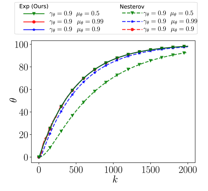
(a) Fixed $\gamma_{\theta}$, varying $\mu_{\theta}$.

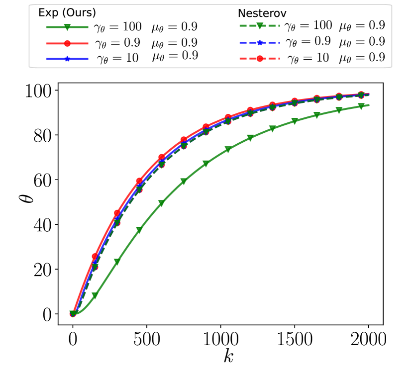
(b) Fixed $\mu_{\theta}$, varying $\gamma_{\theta}$.

Figure 4: The effect of the damping parameter $\gamma_{\theta}$ and momentum coefficient $\mu_{\theta}$ on MPD.

J.4 Experimental Details

Here, we outline for reproducibility the settings: for the Toy Hierarchical Model (Section J.4.1); image generation experiment (Section J.4.2); and, additional figures are in Section J.6. Much akin to Kuntz et al., (2023, Section 2), we found it beneficial to consider separate time-scales for the $(\theta_{t},m_{t})$ and $(X_{t},U_{t})$ which we denote $h_{\theta}$ and $h_{x}$ respectively.

J.4.1 Toy Hierarchical Model

Model The model is described in Kuntz et al., (2023, Example 1). For completeness, we describe it here. The model is defined by

$$p_{\theta}(x,y)=\prod_{i=1}^{d_{x}}\mathcal{N}(y_{i};x_{i},1)\mathcal{N}(x_{i};\theta,\sigma^{2}).$$ (82)

Thus, for the log-likelihood with $\sigma^{2}=1$, we have

$$\log p_{\theta}(x,y)=C-\frac{1}{2}\sum_{i=1}^{d_{x}}\left((x_{i}-\theta)^{2}+(y_{i}-x_{i})^{2}\right),$$

where $C$ is a constant independent of $\theta$ and $x$.

Figure 1(a). For the different regimes, we use the following momentum parameters:

• Underdamped: $\gamma_{\theta}=0.1,\eta_{\theta}=403.96,\gamma_{x}=0.1,\eta_{x}=403.96$

• Overdamped: $\gamma_{\theta}=1,\eta_{\theta}=403.96,\gamma_{x}=1,\eta_{x}=403.96$

• Critically Damped $\gamma_{\theta}=0.7,\eta_{\theta}=403.96,\gamma_{x}=0.7,\eta_{x}=403.96$

The step-sizes are $h_{\theta}=10^{-2}/N=10^{-4}$, $h_{x}=10^{-2}$, with number of samples $N=100$, and number of particles $M=100$.

Figure 1(b). We compare the discretization outlined in Section I.3, and Section 5. We keep all parameters equal except for changing the momentum coefficient $\mu$. For step-sizes, we have $h_{\theta}=10^{-5/2}\approx 5.8\times 10^{-3},h_{x}=10^{-3}$, $\gamma_{x}=\gamma_{\theta}=0.5$, with the momentum coefficient set to $\mu_{\theta}=\mu_{x}=\mu$ where $\mu\in\{0.9,0.8,0.5\}$.

Lipschitz Constant and Strong log concavity. For the toy Hierarchical model with $\sigma^{2}=1$, one can show that it satisfies our Lipschitz assumption, as well as being strongly log-concave. We have

$$\nabla_{(\theta,x)}^{2}\log p_{\theta}=\begin{pmatrix}-d_{x}&1_{1\times d_{x}}\\ 1_{d_{x}\times 1}&-2I_{d_{x}}\\ \end{pmatrix}.$$

The characteristic equation can be written as

$$\det(\nabla_{(\theta,x)}^{2}\log p_{\theta}-lI_{d_{x+1}})=0.$$

The determinant can be evaluated by expanding the minors. Thus, we obtain

$$\det(\nabla_{(\theta,x)}^{2}\log p_{\theta}-lI_{d_{x+1}})= (-d_{x}-l)(-2-l)^{d_{x}}-d_{x}(-2-l)^{d_{x}-1}$$

$$= (-2-l)^{d_{x}-1}((2+l)(d_{x}+l)-d_{x})$$

$$= (-2-l)^{d_{x}-1}(l^{2}+(2+d_{x})l+d_{x}).$$

Hence, the characteristic equation is satisfied when $l\in\{-2,\frac{-(2+d_{x})\pm\sqrt{d_{x}^{2}+4}}{2}\}$. Note that $\frac{-(2+d_{x})-\sqrt{d_{x}^{2}+4}}{2}\leq-2$.

From the above calculations, it can be seen that $\nabla_{(\theta,x)}^{2}\log p_{\theta}$ is strongly-log concave, i.e., we have $\nabla_{(\theta,x)}^{2}\log p_{\theta}\preceq-2I$.

In order to calculate its Lipschitz constant of 1, by Nesterov, (2003, Lemma 1.2.2), this is equivalent to finding a constant $K_{hm}>0$ such that

$$\|\nabla_{(\theta,x)}^{2}\log p_{\theta}\|\leq K_{hm}.$$

Since $\nabla_{(\theta,x)}^{2}\log p_{\theta}$ is symmetric, then the matrix norm is given by the largest absolute value of the eigenvalue of $\nabla_{(\theta,x)}^{2}\log p_{\theta}$ (i.e., it’s spectral radius).

Hence, we have $K_{hm}=\frac{(2+d_{x})+\sqrt{d_{x}^{2}+4}}{2}$.

J.4.2 Image Generation

The dataset of both MNIST and CIFAR-10 is processed similarly. We use $N=5000$ images for training and $3000$ for testing. The model is updated $6280$ times using subsampling with a batch size of $32$. Hence, it completes $40$ epochs. The model is defined as:

$$p_{\theta}(y,x)=\prod_{i=1}^{N}p_{\theta}(y^{i},x^{i}),$$

where:

• The datum $(y^{i},x^{i})\in\mathbb{R}^{d_{y}}\times\mathbb{R}^{d_{x}}$ denotes a single image and its corresponding latent variable. For MNIST, we have $d_{y}=28\times 28=784$ and for CIFAR, we have $d_{y}=32\times 32\times 3=3072$. For both datasets, we set $d_{x}=64$. Thus, we have that $(y,x)\in\mathbb{R}^{d_{y}\times N}\times\mathbb{R}^{d_{x}\times N}$.

• For the VAE model, we have $p(y^{i},x^{i})=\mathcal{N}(y^{i}|g_{\psi}(x^{i}),\sigma^{2}I)p_{\phi}(x^{i})$, where $\psi$ and $\phi$ are parameters of the generator and prior respectively. Thus, the parameter of the model is given by $\theta=\{\psi,\phi\}$. We set $\sigma^{2}=0.1$. The following specifies the details regarding the generator $g_{\psi}$ and prior $p_{\phi}$:

  • Generator $g_{\psi}$. For CIFAR, we use a Convolution Transpose network (as in Pang et al., (2020)) shown in Table 2. For MNIST, we use a fully connected network specified in Table 3 with $d_{in}=d_{x}$ and $d_{out}=d_{y}$.

  • Prior $p_{\phi}(x)$. The prior is inspired by the VampPrior (Tomczak and Welling, , 2018) and is defined as:

    $$p_{\phi}(x)=\frac{1}{K}\sum_{i=1}^{K}\mathcal{N}(x|\mu_{\nu}(z_{i}),\sigma^{2}_{\nu}(z_{i})I_{d_{z}}),$$

    where $\mu_{\nu},\sigma^{2}_{\nu}:\mathbb{R}^{d_{z}}\rightarrow\mathbb{R}^{d_{x}}$ are neural networks (with parameters $\nu$) that parameterized the mean and variance; pseudo-points $\{z_{i}\}_{i=1}^{K}$ are optimized; and so the prior parameters are $\phi:=\{\nu\}\cup\{z_{i}\}_{i=1}^{K}$. The architecture can be found in Table 4 where $d_{in}=d_{z}$ and $d_{out}=d_{z}$

Layers	Size	Stride	Pad
Input	1x1x128	-	-
8x8 ConvT(ngf x 8), LReLU	8x8x(ngf x 8)	1	0
4x4 ConvT(ngf x 4), LReLU	16x16x(ngf x 4)	2	1
4x4 ConvT(ngf x 2), LReLU	32x32x(ngf x 2)	2	1
3x3 ConvT(3), Tanh	32x32x3	1	1

Table 2: Generator network for the VAE used for CIFAR-10 (ngf = 256).

Layers	Size
Input	$d_{x}$
Linear($d_{x}$, 512), LReLU	512
Linear(512,512), LReLU	512
Linear(512,512), LReLU	512
Linear(512,$d_{y}$), Tanh	$d_{y}$

Table 3: Generator network for the VAE used for MNIST.

Layers	Size
Input	$d_{in}$
Linear($d_{in}$, 512), LReLU	512
Linear(512,512), LReLU	512
Linear(512,512), LReLU	512
Linear(512,$d_{out}\times 2$)	$d_{out}\times 2$
Output: Id([:$d_{out}$]), Softplus([$d_{out}$:])	$d_{out},d_{out}$

Table 4: Neural network parametrization of the mean and variance of a Gaussian Distribution used in VI and VAMPprior. “Id” is the identity function, and “[:$d_{out}$]” is a standard pseudo-code notation that refers to the operation that extracts the first $d_{out}$ dimensions and similarly for [$d_{out}$:].

J.5 Hyperparameter settings

Unless specified otherwise, we use the same parameters for both MNIST and CIFAR datasets. Our approach to selecting the step size involved first setting it to $10^{-3}$, then we would decrease it appropriately if instabilities arise.

• MPD. For step sizes, we have $h_{\theta}=h_{x}=10^{-4}$. The number of particles is set to $M=5$. For the momentum parameters, we use $\gamma_{\theta}=\gamma_{x}=0.9$ with the momentum coefficient $\mu_{\theta}=0.95,\mu_{x}=0$ (or equivalently, $\eta_{\theta}\approx 556,\eta_{x}\approx 11,111$ )for MNIST and $\mu_{\theta}=0.95,\mu_{x}=0.5$ (or equivalently, $\eta_{\theta}\approx 556,,\eta_{x}\approx 55,555$ ) for CIFAR. We use the RMSProp preconditioner (see Section J.1) with $\beta=0.9$.

• PGD. We have $h_{\theta}=10^{-4},h_{x}=10^{-3}$. The number of particles is set to $M=5$. We use the RMSProp preconditioner (see Section J.1) with $\beta=0.9$.

• ABP. We use SGD optimizer with step size $h_{\theta}=10^{-4}$, and run a length $5$ ULA chain $5$ with step-size $h_{x}=10^{-3}$. We found that RMSProp worked well in the transient period but failed to achieve better performance than SGD.

• SR. We used RMSProp optimizer with step size $h_{\theta}=10^{-4}$, and ran five $20$-length ULA chain with step-size $h_{x}=10^{-3}$

• VI. We use RMSProp optimizer with a step size of $h=10^{-5}$. We found that this resulted in the best performance. For the encoder, we use a Mean Field approximation as in Kingma and Welling, (2014). The neural network is a $3$-layer fully connected network with Leaky Relu activation functions. In the last layer, we use a softmax to parameterize the variance. See Table 4.

J.6 Additional Figures

Appendix K Additional Experiments

In this section, we show additional experiments particularly concerned with comparing MPD with PGD and other variants of MPD that only accelerated one component of the space instead of two. We say $X$-enriched to indicate algorithms with momentum incorporated in $X$ with either momentum included/excluded in $\theta$. To separate the two cases, we call $X$-only-enriched to refer to the algorithm with gradient descent in $\theta$. We use similar terminology for $\theta$-enriched and $\theta$-only-enriched.

We consider two settings: in Section K.1, further results with the toy Hierarchical model (see Section J.4.1); and, in Section K.2 a density estimation task using VAEs on a Mixture of Gaussian dataset.

K.1 Toy Hierarchical Model

Figure 7. As the model, we consider a Toy Hierarchical model for different $\sigma$ values in (82) where $\sigma$ is chosen to be the same as the data generating process. The data is generated from a toy Hierarchical model with parameters $(\theta=10,\sigma)$ where $\sigma=\{5,10,12\}$. As noted by Kuntz et al., (2023, Eq. 51), the marginal maximum likelihood of $\theta$ is the empirical average of the observed samples, i.e., $\frac{1}{d_{x}}\sum_{i=1}^{d_{x}}y_{i}$. For each trial, we process the data $(y_{i})_{i=1}^{d_{x}}$ to have an empirical average of $10$ for simplicity.

Figure 2(a), Figure 2(b), Figure 2(c) We use a toy Hierarchical model with $\sigma=12$, and, similarly, the data-generating processing is a toy Hierarchical model with $(\theta=10,\sigma=12)$. We are interested in how the initialization of the particle cloud affects MPD, PGD and other algorithms that only momentum-enriched one component. Each subplot shows the evolution of the parameter $\theta$ for the initialization from $\mathcal{N}(\mu,I)$ where $\mu\in\{-5,-20,-100\}$. This example serves as an illustration of the typical case where the cloud is initialized badly. It can be seen that all methods are affected by poor initialization. For $X$-enriched, the algorithms can recover faster to achieve almost identical performances (at the later iterations) between different initializations. In other words, for $X$-enriched algorithms transient phase is short. Methods without such $X$-enrichment take longer to recover and are unable to achieve similar performances compared to the cases where they are better-initialized. Overall, it can be seen that MPD perform better than PGD.

(a) $\sigma=5$.

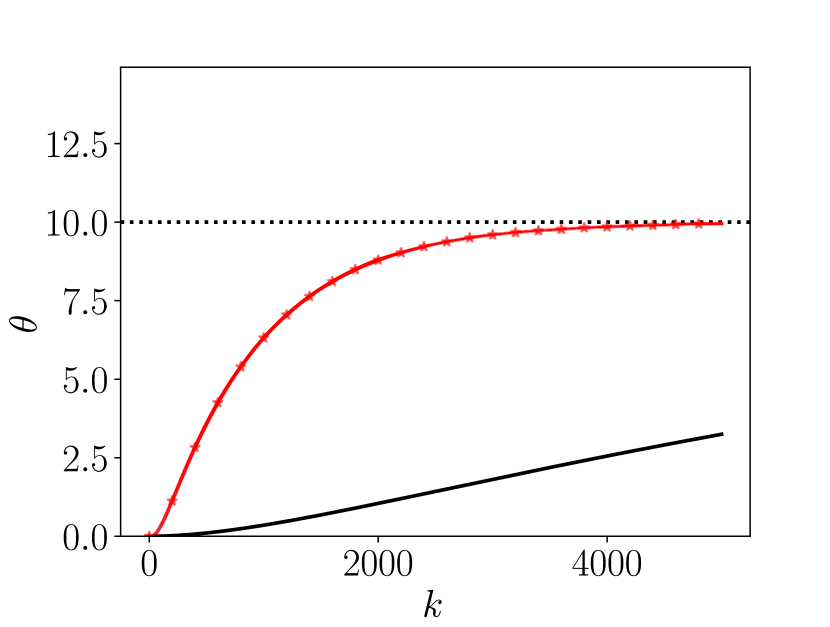
(b) $\sigma=10$.

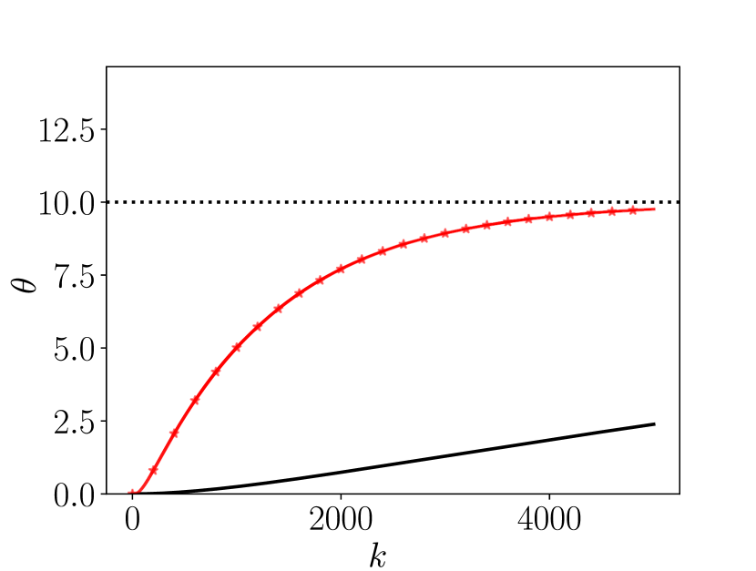
(c) $\sigma=12$.

Figure 7: Comparison between MPD and PGD on the Toy Hierarchical Model for different choices of $\sigma$. The plot shows the average and standard deviation of $\theta$ across iterations computed over $10$ independent trials. MPD is shown in red and PGD in black. The dashed line shows the true value.

K.2 Density Estimation

In this problem, we show the result of training a VAE with VAMP Prior on a 1-d Mixture of Gaussians (MoG) dataset with PDF shown in Figure 8. The dataset is composed of $100$ samples. In Figure 2(d), we show the performance of various acceleration algorithms. The empirical Wasserstein-1 distance (denoted by $\hat{\mathsf{W}}_{1}$) is estimated from the empirical CDF produced from $1000$ samples across each iteration. The results show the average (with standard error bars which are barely noticeable) computed over $100$ trials. PGD is shown in black, and MPD is shown in green. In this case, all accelerated algorithms perform better than PGD, and MPD performs best of all.

Hyperparameters: No subsampling used. We have $d_{y}=1,d_{x}=10$. We set $\gamma_{x}=\gamma_{\theta}=0.4$, and use the momentum heuristic with $\mu_{\theta}=\mu_{x}=0.1$ (see Section J.3). We use the same VAE architecture in Section J.4.2 with likelihood noise $\sigma=0.01$, an MLP decoder (see Table 4), and VAMP prior with $d_{z}=2$ and $K=20$.

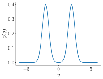
Figure 8: The true density of the MoG dataset.

References

• Ambrosio et al., (2005) Ambrosio, L., Gigli, N., and Savaré, G. (2005). Gradient flows: in metric spaces and in the space of probability measures. Springer Science & Business Media.
• Andrieu and Thoms, (2008) Andrieu, C. and Thoms, J. (2008). A tutorial on adaptive MCMC. Statistics and computing, 18:343–373.
• Bakry and Émery, (2006) Bakry, D. and Émery, M. (2006). Diffusions hypercontractives. In Séminaire de Probabilités XIX 1983/84: Proceedings, pages 177–206. Springer.
• Bernton, (2018) Bernton, E. (2018). Langevin Monte Carlo and JKO splitting. In Conference on learning theory, pages 1777–1798. PMLR.
• Carmona, (2016) Carmona, R. (2016). Lectures on BSDEs, stochastic control, and stochastic differential games with financial applications. SIAM.
• Chen et al., (2022) Chen, F., Ren, Z., and Wang, S. (2022). Uniform-in-time propagation of chaos for mean field langevin dynamics. arXiv preprint arXiv:2212.03050.
• Cheng et al., (2018) Cheng, X., Chatterji, N. S., Bartlett, P. L., and Jordan, M. I. (2018). Underdamped Langevin MCMC: A non-asymptotic analysis. In Conference on Learning Theory, pages 300–323. PMLR.
• Chizat, (2022) Chizat, L. (2022). Mean-field Langevin dynamics: Exponential convergence and annealing. arXiv preprint arXiv:2202.01009.
• Chizat and Bach, (2018) Chizat, L. and Bach, F. (2018). On the global convergence of gradient descent for over-parameterized models using optimal transport. Advances in neural information processing systems, 31.
• De Bortoli et al., (2021) De Bortoli, V., Durmus, A., Pereyra, M., and Vidal, A. F. (2021). Efficient stochastic optimisation by unadjusted Langevin Monte Carlo: Application to maximum marginal likelihood and empirical Bayesian estimation. Statistics and Computing, 31:1–18.
• Delyon et al., (1999) Delyon, B., Lavielle, M., and Moulines, E. (1999). Convergence of a stochastic approximation version of the EM algorithm. Annals of statistics, pages 94–128.
• Diao et al., (2023) Diao, M. Z., Balasubramanian, K., Chewi, S., and Salim, A. (2023). Forward-backward Gaussian variational inference via JKO in the Bures-Wasserstein space. In International Conference on Machine Learning, pages 7960–7991. PMLR.
• Dockhorn et al., (2022) Dockhorn, T., Vahdat, A., and Kreis, K. (2022). Score-based generative modeling with critically-damped Langevin diffusion. In International Conference on Learning Representations (ICLR).
• Duncan et al., (2023) Duncan, A., Nüsken, N., and Szpruch, L. (2023). On the geometry of Stein variational gradient descent. Journal of Machine Learning Research, 24(56):1–39.
• Garbuno-Inigo et al., (2020) Garbuno-Inigo, A., Nüsken, N., and Reich, S. (2020). Affine invariant interacting Langevin dynamics for Bayesian inference. SIAM Journal on Applied Dynamical Systems, 19(3):1633–1658.
• Gelfand and Silverman, (2000) Gelfand, I. M. and Silverman, R. A. (2000). Calculus of Variations. Courier Corporation.
• Good, (1983) Good, I. J. (1983). Good thinking: The foundations of probability and its applications. University of Minnesota Press.
• Han et al., (2017) Han, T., Lu, Y., Zhu, S.-C., and Wu, Y. N. (2017). Alternating back-propagation for generator network. In Proceedings of the AAAI Conference on Artificial Intelligence, volume 31.
• Heusel et al., (2017) Heusel, M., Ramsauer, H., Unterthiner, T., Nessler, B., and Hochreiter, S. (2017). GANs trained by a two time-scale update rule converge to a local nash equilibrium. Advances in Neural Information Processing Systems, 30.
• Hinton, (2002) Hinton, G. E. (2002). Training products of experts by minimizing contrastive divergence. Neural computation, 14(8):1771–1800.
• Hochbruck and Ostermann, (2010) Hochbruck, M. and Ostermann, A. (2010). Exponential integrators. Acta Numerica, 19:209–286.
• Hu et al., (2021) Hu, K., Ren, Z., Šiška, D., and Szpruch, Ł. (2021). Mean-field Langevin dynamics and energy landscape of neural networks. In Annales de l’Institut Henri Poincare (B) Probabilites et statistiques, volume 57, pages 2043–2065. Institut Henri Poincaré.
• Jordan et al., (1998) Jordan, R., Kinderlehrer, D., and Otto, F. (1998). The variational formulation of the Fokker–Planck equation. SIAM Journal on Mathematical Analysis, 29(1):1–17.
• Kac, (1956) Kac, M. (1956). Foundations of kinetic theory. In Proceedings of The third Berkeley symposium on mathematical statistics and probability, volume 3, pages 171–197.
• Kingma and Welling, (2014) Kingma, D. P. and Welling, M. (2014). Auto-encoding variational Bayes. In Bengio, Y. and LeCun, Y., editors, 2nd International Conference on Learning Representations, ICLR 2014, Banff, AB, Canada, April 14-16, 2014, Conference Track Proceedings.
• Krizhevsky and Hinton, (2009) Krizhevsky, A. and Hinton, G. (2009). Learning multiple layers of features from tiny images.
• Kruger, (2003) Kruger, A. Y. (2003). On Fréchet subdifferentials. Journal of Mathematical Sciences, 116(3):3325–3358.
• Kuntz et al., (2023) Kuntz, J., Lim, J. N., and Johansen, A. M. (2023). Particle algorithms for maximum likelihood training of latent variable models. In Proceedings on 26th International Conference on Artificial Intelligence and Statistics (AISTATS), volume 206 of Proceedings of Machine Learning Research, pages 5134–5180.
• Lambert et al., (2022) Lambert, M., Chewi, S., Bach, F., Bonnabel, S., and Rigollet, P. (2022). Variational inference via wasserstein gradient flows. Advances in Neural Information Processing Systems, 35:14434–14447.
• LeCun et al., (1998) LeCun, Y., Bottou, L., Bengio, Y., and Haffner, P. (1998). Gradient-based learning applied to document recognition. Proceedings of the IEEE, 86(11):2278–2324.
• Liu, (2017) Liu, Q. (2017). Stein variational gradient descent as gradient flow. Advances in Neural Information Processing Systems, 30.
• Loève, (1977) Loève, M. (1977). Probability Concepts, pages 151–176. Springer New York, New York, NY.
• Ma et al., (2021) Ma, Y.-A., Chatterji, N. S., Cheng, X., Flammarion, N., Bartlett, P. L., and Jordan, M. I. (2021). Is there an analog of Nesterov acceleration for gradient-based MCMC? Bernoulli, 27(3):1942 – 1992.
• Maddison et al., (2018) Maddison, C. J., Paulin, D., Teh, Y. W., O’Donoghue, B., and Doucet, A. (2018). Hamiltonian descent methods. arXiv preprint arXiv:1809.05042.
• Martens, (2010) Martens, J. (2010). Deep learning via Hessian-free optimization. In International Conference on Machine Learning, volume 27, pages 735–742.
• McCall, (2010) McCall, M. W. (2010). Classical Mechanics: From Newton to Einstein: A Modern Introduction. John Wiley & Sons.
• McKean Jr, (1966) McKean Jr, H. P. (1966). A class of Markov processes associated with nonlinear parabolic equations. Proceedings of the National Academy of Sciences, 56(6):1907–1911.
• McLachlan and Perlmutter, (2001) McLachlan, R. and Perlmutter, M. (2001). Conformal Hamiltonian systems. Journal of Geometry and Physics, 39(4):276–300.
• Mei et al., (2018) Mei, S., Montanari, A., and Nguyen, P.-M. (2018). A mean field view of the landscape of two-layer neural networks. Proceedings of the National Academy of Sciences, 115(33):E7665–E7671.
• Neal and Hinton, (1998) Neal, R. M. and Hinton, G. E. (1998). A view of the EM algorithm that justifies incremental, sparse, and other variants. Learning in graphical models, pages 355–368.
• Nemirovskij and Yudin, (1983) Nemirovskij, A. S. and Yudin, D. B. (1983). Problem complexity and method efficiency in optimization. Wiley-Interscience.
• Nesterov, (2003) Nesterov, Y. (2003). Introductory Lectures on Convex Optimization: A Basic Course. Springer Science & Business Media.
• Nesterov, (1983) Nesterov, Y. E. (1983). A method of solving a convex programming problem with convergence rate $\mathcal{O}\bigl{(}\frac{1}{k^{2}}\bigr{)}$. In Doklady Akademii Nauk, volume 269, pages 543–547. Russian Academy of Sciences.
• Nijkamp et al., (2020) Nijkamp, E., Pang, B., Han, T., Zhou, L., Zhu, S.-C., and Wu, Y. N. (2020). Learning multi-layer latent variable model via variational optimization of short run MCMC for approximate inference. In Computer Vision–ECCV 2020: 16th European Conference, Glasgow, UK, August 23–28, 2020, Proceedings, Part VI 16, pages 361–378. Springer.
• Nitanda and Suzuki, (2017) Nitanda, A. and Suzuki, T. (2017). Stochastic particle gradient descent for infinite ensembles. arXiv preprint arXiv:1712.05438.
• Nitanda et al., (2022) Nitanda, A., Wu, D., and Suzuki, T. (2022). Convex analysis of the mean field Langevin dynamics. In International Conference on Artificial Intelligence and Statistics, pages 9741–9757. PMLR.
• Otto and Villani, (2000) Otto, F. and Villani, C. (2000). Generalization of an Inequality by Talagrand and Links with the Logarithmic Sobolev Inequality. Journal of Functional Analysis, 173(2):361–400.
• O’Donoghue and Candes, (2015) O’Donoghue, B. and Candes, E. (2015). Adaptive restart for accelerated gradient schemes. Foundations of Computational Mathematics, 15:715–732.
• Pang et al., (2020) Pang, B., Han, T., Nijkamp, E., Zhu, S.-C., and Wu, Y. N. (2020). Learning latent space energy-based prior model. Advances in Neural Information Processing Systems, 33:21994–22008.
• Peyré and Cuturi, (2019) Peyré, G. and Cuturi, M. (2019). Computational optimal transport: With applications to data science. Foundations and Trends in Machine Learning, 11(5-6):355–607.
• Platen and Bruti-Liberati, (2010) Platen, E. and Bruti-Liberati, N. (2010). Numerical Solution of Stochastic Differential Equations with Jumps in Finance. Springer Science & Business Media.
• Riou-Durand et al., (2023) Riou-Durand, L., Sountsov, P., Vogrinc, J., Margossian, C., and Power, S. (2023). Adaptive tuning for Metropolis adjusted Langevin trajectories. In International Conference on Artificial Intelligence and Statistics, pages 8102–8116. PMLR.
• Roberts and Rosenthal, (2009) Roberts, G. O. and Rosenthal, J. S. (2009). Examples of adaptive MCMC. Journal of computational and graphical statistics, 18(2):349–367.
• Santambrogio, (2017) Santambrogio, F. (2017). $\{$Euclidean, metric, and Wasserstein$\}$ gradient flows: an overview. Bulletin of Mathematical Sciences, 7:87–154.
• Sanz-Serna and Zygalakis, (2021) Sanz-Serna, J. M. and Zygalakis, K. C. (2021). Wasserstein distance estimates for the distributions of numerical approximations to ergodic stochastic differential equations. The Journal of Machine Learning Research, 22(1):11006–11042.
• Sharrock and Nemeth, (2023) Sharrock, L. and Nemeth, C. (2023). Coin sampling: Gradient-based Bayesian inference without learning rates. In Krause, A., Brunskill, E., Cho, K., Engelhardt, B., Sabato, S., and Scarlett, J., editors, Proceedings of the 40th International Conference on Machine Learning, volume 202 of Proceedings of Machine Learning Research, pages 30850–30882. PMLR.
• Shi et al., (2021) Shi, B., Du, S. S., Jordan, M. I., and Su, W. J. (2021). Understanding the acceleration phenomenon via high-resolution differential equations. Mathematical Programming, 195:79–148.
• Silvester, (2000) Silvester, J. R. (2000). Determinants of block matrices. The Mathematical Gazette, 84(501):460–467.
• Staib et al., (2019) Staib, M., Reddi, S., Kale, S., Kumar, S., and Sra, S. (2019). Escaping saddle points with adaptive gradient methods. In International Conference on Machine Learning, pages 5956–5965. PMLR.
• Su et al., (2014) Su, W., Boyd, S., and Candes, E. (2014). A differential equation for modeling Nesterov’s accelerated gradient method: theory and insights. Advances in Neural Information Processing Systems, 27.
• Sutskever et al., (2013) Sutskever, I., Martens, J., Dahl, G., and Hinton, G. (2013). On the importance of initialization and momentum in deep learning. In International Conference on Machine Learning, pages 1139–1147. PMLR.
• Suzuki et al., (2023) Suzuki, T., Wu, D., and Nitanda, A. (2023). Convergence of mean-field Langevin dynamics: Time and space discretization, stochastic gradient, and variance reduction. arXiv preprint arXiv:2306.07221.
• Tieleman and Hinton, (2012) Tieleman, T. and Hinton, G. (2012). Lecture 6.5-rmsprop, coursera: Neural networks for machine learning. University of Toronto, Technical Report, 6.
• Tomczak and Welling, (2018) Tomczak, J. and Welling, M. (2018). VAE with a VampPrior. In International Conference on Artificial Intelligence and Statistics, pages 1214–1223. PMLR.
• Van Handel, (2014) Van Handel, R. (2014). Probability in high dimension. Lecture Notes (Princeton University).
• Villani, (2009) Villani, C. (2009). Optimal transport: old and new, volume 338. Springer.
• Wibisono, (2018) Wibisono, A. (2018). Sampling as optimization in the space of measures: The Langevin dynamics as a composite optimization problem. In Conference on Learning Theory, pages 2093–3027. PMLR.
• Wibisono et al., (2016) Wibisono, A., Wilson, A. C., and Jordan, M. I. (2016). A variational perspective on accelerated methods in optimization. Proceedings of the National Academy of Sciences, 113(47):E7351–E7358.
• Wilson et al., (2016) Wilson, A. C., Recht, B., and Jordan, M. I. (2016). A Lyapunov analysis of momentum methods in optimization. arXiv preprint arXiv:1611.02635.
• Yao and Yang, (2022) Yao, R. and Yang, Y. (2022). Mean field variational inference via Wasserstein gradient flow. arXiv preprint arXiv:2207.08074.
\appendixpage\startcontents
[sections] \printcontents[sections]l1