Linear and nonlinear clusterings of Horndeski-inspired dark energy models with fast transition

Abstract

We analyze time-dependent dark energy equations of state through linear and nonlinear structure formation and their quintessence potentials, characterized by fast, recent transitions, inspired by parameter space studies of Horndeski models. The influence of dark energy on structures comes from modifications to the background expansion rate and from perturbations as well. In order to compute the structures growth, we employ a generalization of the spherical collapse formalism that includes perturbations of fluids with pressure. We numerically solve the equations of motion for the perturbations and the field. Our analysis suggests that a true Heaviside step transition is a good approximation for most of the considered models, since most of the quantities weakly depend on the transition speed. We find that transitions occurring at redshifts $z_{\rm t}\gtrsim 2$ cannot be distinguished from the $\Lambda$CDM model if dark energy is freezing, i.e., the corresponding equation of state tends to $-1$. For fast, recent transitions, the redshift at which the properties of dark energy have the most significant effect is $z=0.6\pm 0.2$. We also find that in the freezing regime, the $\sigma_{8}$ values can be lowered by about $8\%$, suggesting that those models could relieve the $\sigma_{8}$-tension. Additionally, freezing models generally predict faster late-time merging rates but a lower number of massive galaxies at $z=0$. Finally, the matter power spectrum for smooth dark energy shows a low-wavenumber peak which is absent in the clustering case.

I Introduction

Experimental evidences favor a late-time cosmic acceleration [1, 2, 3] and suggest the existence of an exotic fluid, exhibiting a negative equation of state (EOS), called dark energy (DE). In the standard cosmological puzzle, DE is intimately related to the cosmological constant, $\Lambda$, arising from vacuum energy quantum fluctuations [4, 5].

Generally, two different possibilities are commonly developed to explain the fundamental nature of DE. The first is framing out the EOS, $w(z)$, through parametric functions of redshift and observationally constraining its evolution [10, 11]. The second is deriving the DE EOS from first principles, making a priori hypotheses on its microphysics [12].

In this respect, the use of field theories appears of utmost importance to model DE in terms of its intrinsic constituent. Specifically, the most general scalar-tensor theory of gravitation in four dimensions remains the Horndeski theory [15], incorporating limiting cases such as quintessence or $k$-essence. In those models, the EOS naturally arises from the scalar field and, so, describing DE through Horndeski models implies that the EOS reconstruction with data determines constraints on the corresponding scalar field potential.

At small redshifts, the majority of DE models fully degenerates [17], indicating that late-time constraints appear less predictive in clarifying how DE evolves throughout the universe evolution [18, 19]. Nevertheless, DE exerts its influence through its impact on cosmic perturbations. Accordingly, it significantly affects the rate of formation and growth of virialized structures, such as galaxies, galaxy clusters, and more. Indeed, the cosmic expansion, if driven by DE, acts to decelerate the gravitational collapse of overdense regions through the Hubble drag. As DE becomes dominant, overdense regions experience slower growth, and the matter gravitational collapse may even reverse on scales comparable to the Hubble horizon.

Particularly, if DE is not the cosmological constant, it could exhibit fluctuations in both space and time. Consequently, DE is not only influenced by matter overdensities but also gives rise to its own overdensities, that, in turn, exert a nonlinear influence on matter overdensities.

Motivated by the aforementioned points, in this work we analyze how effective DE fluid models, characterized by an EOS with fast transitions, affect the background evolution and structure formation. This class of paradigms is still under study and far from being rejected as suitable candidate for DE [20, 21, 22, 23, 24]. While in previous efforts a given parametrization has been investigated, in this work we analyze six different parameterizations, four of which belong to the same fast transition class, in order to understand if the models can be distinguished from one another and from the $\Lambda$CDM scenario. Accordingly, we determine their effects on structures’ growth by employing a generalization of the spherical collapse formalism that includes fluids with pressure, adopting the formalism developed in [25, 26]. We then numerically solve the equations of motion (EOM) of the perturbation and field and investigate linear and nonlinear features of our models. As a key output, our analysis seems to suggest that a true Heaviside step transition works fairly well as an alternative to the cosmological constant and provide a good approximation to fast transition models. Even though promising, we emphasize that transitions happening at $z\geq 2$ cannot be distinguished from the standard cosmological model, if DE is freezing. Particularly, in the freezing regime, slight improvements on the $\sigma_{8}$ tension can be achieved, roughly indicating that such field models may in principle heal this cosmic tension. Finally, the matter power spectrum for smooth DE shows a low-wave number peak which is absent in the clustering case.

The paper is structured as follows. In Sec. II we work out how DE can be described in a scalar tensor theory and introduce the Horndeski theory. In Sec. II.2, we specialize to the effective fluid description of quintessence theory. In Sec. III we set the perturbation framework, introducing the spherical collapse formalism, the pseudo Newtonian approximation to gravitational interaction. Sec. IV is devoted to the analysis of the fast transition models. After a brief introduction to the models, we begin the analysis computing numerically the quintessence potential and field that correspond to each EOS. We then compute the linear matter perturbations and make extensive use of numerical simulations to compute the virialization overdensity and the linearly extrapolated density contrast at collapse for the matter perturbations. These quantities allow for a semi-quantitative analysis of the models and are needed to compute the halo mass function (HMF) in Sec. IV.7. The HMF is quite an important quantity as it can be directly compared to results of large $N$-body cosmological simulations and will be hopefully measured accurately by the Euclid survey [27]. Conclusions and perspectives are discussed in Sec. V. Throughout this article, we will assume $c=1$.

II From scalar to Horndeski theories

While general relativity is the most successful theory for explaining gravity, alternatives have been introduced and severely investigated. To do so, one approach is introducing an additional scalar field, that, in the simplest version, is given by

$$\mathcal{L}_{\phi}=-\frac{1}{2}\nabla_{\mu}\phi\nabla^{\mu}\phi-V(\phi)\,.$$ (1)

Consequently, the Lagrangian density includes a further term, contributing to the energy-momentum tensor, within the Einstein-Hilbert action

$$S=\int_{\mathcal{D}}\mathrm{d}^{4}x\,\sqrt{-g}\,(\mathcal{L}_{\rm EH}+\mathcal{L}_{\phi})\,,$$

where $g$ stands for the determinant of the metric, while $\mathcal{L}_{\rm EH}$ is the Einstein-Hilbert Lagrangian and $\mathcal{D}$ the integration domain.

The usual Klein-Gordon equation of motion (EOM) for the field holds, and reduces in a Friedmann-Robertson-Walker (FRW) universe to

$$\ddot{\phi}+3H\dot{\phi}+\frac{\partial V}{\partial\phi}=0\,.$$ (2)

This cosmological scalar field is known as quintessence, representing an example of a minimally-coupled scalar tensor theory, i.e., gravity and the scalar field are coupled only through the metric tensor, emerging when we are contracting indices.

To include conventional matter, the procedure is analogous and derives from the additivity property of Lagrangian.

II.1 Horndeski theories

Scalar tensor theories represent a powerful instrument to produce self-consistent modified theories of gravity. According to Lovelock’s theorem, Einstein equations are the only possible second-order Euler-Lagrange equations derived from a Lagrangian scalar density in $3+1$ dimensions that is constructed solely from the metric, $\mathcal{L}=\mathcal{L}(g\indices{{}_{\mu}{}_{\nu}})$ [31]. To extend Einstein’s theory of gravity, we can relax this hypothesis of Lovelock’s theorem. A simple way to do this, is to add another degree of freedom different from the metric, e.g. a scalar field. In so doing, the EOM contain higher order derivatives, possibly leading to Ostrogradsky instabilities [15].

The Horndeski theory is also known, for historical reasons, as the generalized covariant Galileon [32]. The procedure to obtain the Horndeski theory is to start from the most general scalar field theory on a Minkowsky spacetime, which yields second order equations, under the assumptions that the Lagrangian contains at most second order derivatives of the field, behaving as polynomial in $\partial_{\mu}\partial_{\nu}\phi$.

One then promotes the theory to be covariant, replacing partial derivatives with covariant derivatives, and adds appropriate unique counterterms to retain second order field equations. The overall procedure can be realized in any dimensions and, particularly, in four the Horndeski theory is given by [15, 33, 34]

$$\mathcal{L}= \,G_{2}(\phi,X)-G_{3}(\phi,X)\Box\phi+G_{4}(\phi,X)R+$$ (3)

$$\,G_{4X}\left[\left(\Box\phi\right)^{2}-\phi\indices{{}^{\mu}{}^{\nu}}\phi\indices{{}_{\mu}{}_{\nu}}\right]+G_{5}(\phi,X)G\indices{{}^{\mu}{}^{\nu}}\phi\indices{{}_{\mu}{}_{\nu}}$$

$$\,-\frac{G_{5X}}{6}X\left[\left(\Box\phi\right)^{3}-3\Box\phi\phi\indices{{}^{\mu}{}^{\nu}}\phi\indices{{}_{\mu}{}_{\nu}}+2\phi\indices{{}_{\mu}{}_{\nu}}\phi\indices{{}^{\nu}{}^{\lambda}}\phi\indices{{}^{\mu}_{\lambda}}\right]\,,$$

where $\phi_{\mu}\equiv\nabla_{\mu}\phi$, $\phi\indices{{}_{\mu}{}_{\nu}}\equiv\nabla_{\mu}\nabla_{\nu}\phi$, $X=-g\indices{{}^{\mu}{}^{\nu}}\phi_{\mu}\phi_{\nu}/2$. $G_{2}$, $G_{3}$, $G_{4}$ and $G_{5}$ are arbitrary functions, playing the role of superpotentials, and depend on $\phi$ and $X$ and, finally, $f_{X}=\partial f/\partial X$. Eq. (3) is the most general scalar-tensor theory exhibiting second-order field equations in four dimensions.

Remarkably, we intend to mime the DE effects within the context of Horndeski theory and check how the so-obtained Horndeski DE influences structure formation, with the hypothesis of fast transition.

II.2 Quintessence as effective fluid

Quintessence models are a subclass of the Horndeski theories. Indeed, minimally coupled quintessence is obtained by setting $G_{3}=G_{5}=0$, $G_{2}=X-V(\phi)$ and $G_{4}=1/(16\pi G)$.

We now want to bridge the gap between the fluid description of DE and its quintessence interpretation. By effective fluid description, we mean to describe DE through its EOS only. In so doing, there are two main approaches:

• We can specify a potential $V(\phi)$ and then derive the EOS, $w$.

• We can alternatively fix the EOS and calculate the corresponding quintessence potential.

We will follow the latter approach. Thus we suppose that the EOS is a given function $w(a)$ [16]. The contact point between fluid and quintessence descriptions is the EOS $w(a)$. We therefore start from its expression in terms of the quintessence field

$$w(\phi,\dot{\phi})=\frac{\frac{\dot{\phi}^{2}}{2}-V(\phi)}{\frac{\dot{\phi}^{2}}{2}+V(\phi)}=\frac{P_{\phi}}{\rho_{\phi}}\,.$$

Thus we have to design the potential in a way that this expression gives the desired $w(a)$. The field satisfies the EOM, that is equivalent to the continuity equation $\dot{\rho}_{\phi}+3H\rho_{\phi}(1+w)=0$. By changing the differentiation variable from $t$ to $a$ and integrating, we obtain

$$\rho_{\phi}=\rho_{0\phi}e^{-3\int_{1}^{a}\frac{1+w(x)}{x}\mathrm{d}x}\coloneqq\rho_{0\phi}g(a)\,.$$

Consequently, the potential reads

$$V(a)=\frac{\rho_{0\phi}}{2}g(a)[1-w(a)]\,,$$ (4)

and, so, to convert $V(a)$ into $V(\phi)$, we need to compute $\phi(a)$, which is given by

$$\phi(a)-\phi_{0}=\pm\sqrt{\frac{3}{8\pi G}}\int_{1}^{a}\mathrm{d}x\,\frac{\sqrt{\Omega^{0}_{\phi}g(x)\left[1+w(x)\right]}}{x\sqrt{\frac{\Omega^{0}_{\rm m}}{x^{3}}+\Omega^{0}_{\phi}g(x)}}\,,$$ (5)

where $\phi_{0}$ is the integration constant. We will select it to ensure that $\phi(a_{\rm min})=0$. In this context, $a_{\rm min}$ denotes the smallest scale parameter value that we employ in our numerical integration.

There are very few cases in which the solution for $g(a)$ is analytical, but if we have an analytic $g(a)$, there are some cases in which $\phi(a)$ can be computed. Even though this can be possible, generally it is not trivial to invert $\phi(a)$ to obtain $a(\phi)$ and, therefore, this task should be numerically computed.

By defining

$$\tilde{V}\equiv\frac{16\pi G}{3H_{0}^{2}}V\,,\quad\quad\tilde{\phi}\equiv\sqrt{\frac{8\pi G}{3}}\phi\,,$$ (6)

we have the dimensionless quantities

$$\tilde{V}(a)= \,\Omega^{0}_{\phi}g(a)[1-w(a)]\,,$$ (7)

$$\tilde{\phi}(a)= \,\pm\int_{1}^{a}\frac{\sqrt{\Omega^{0}_{\phi}g(x)\left[1+w(x)\right]}}{x\sqrt{\frac{\Omega^{0}_{\rm m}}{x^{3}}+\Omega^{0}_{\phi}g(x)}}\mathrm{d}x\,,$$ (8)

that can easily be integrated through numerical methods.

III Perturbations framework

In this section we set the framework to study both linear and nonlinear perturbations in DE models described by a given EOS $w(a)$. Because linear equations can be obtained by linearising the full nonlinear equations, we will not repeat the derivation twice, but we will start directly from the nonlinear equations and then obtain, in the appropriate limit, the linear ones. In addition, we will consider two rather different cases regarding the evolution of perturbations in DE models: one where the DE fluid affects the background only (smooth models) and the other where also the DE component can have perturbations (clustering models). In the latter case, we also need to consider the effects of pressure perturbations.

Investigating perturbations beyond the linear approximation poses significant mathematical difficulties. To tackle these caveats, large numerical simulations are often considered and the spherical collapse model is one of the most used approximation. The model describes the dynamics of an isolated, spherical region of matter, that is collapsing under its own gravitational pull. This model provides a simple, yet effective framework for analyzing the growth of density perturbations in the early universe and their eventual evolution into bound structures such as galaxies and galaxy clusters.

Heuristically, what is requested in the spherical collapse model is to pop into existence an overdense sphere, very early in the cosmic history. Since the universe is expanding, initially the sphere expands with the Hubble flow. However, the overdensity causes an inward gravitational pull that resists the Hubble flow. At a certain point, dubbed turnaround, the sphere radius stops growing. After turnaround the sphere starts collapsing on itself until it reaches zero radius and infinite density. In the physical world, the shrinking stops before the collapse due to non spherical symmetry, peculiar velocities of the particles, friction, pressure and other effects that are ignored in the most basic formulation of the spherical collapse model. To overcome some of those shortcomings, it is assumed that the sphere reaches a time in which it becomes stable and gets into virial equilibrium.

III.1 Spherical collapse model

To grasp the development of nonlinear perturbations in a realistic two-component universe that contains DE, fully-characterized by $w$, and matter, one can extend the Newtonian theory to incorporate DE, as an additional term in the acceleration equation [26, 35, 25].

To do so, we define $\delta_{i}\equiv(\rho_{i}-\bar{\rho}_{i})/\bar{\rho}_{i}$ as the density contrast of the $i$-th fluid, where $\rho_{i}(\boldsymbol{x},t)$ represents the perturbed density, $\bar{\rho}_{i}(t)$ denotes its background density and $\theta_{i}\equiv\nabla\cdot\mathbf{v}_{i}$ the divergence of the peculiar velocity $\mathbf{v}_{i}$. While, in principle, we can have a peculiar velocity for each perturbed species, in our setting this does not happen as the Euler equation is the same for all the species, in our case dark matter and DE.

With respect to standard dark matter perturbations, we need to take into account the fact that DE perturbations involve both density and pressure perturbations. This introduces, therefore, an additional degree of freedom to the model, which can only be set once one knows the micro-physics of the fluid via its Lagrangian formulation. As from a given EOS it is not possible to infer the Lagrangian, unless one specifies the type of DE model a priori, i.e., quintessence or $k$-essence, we take the common ansatz of relating pressure perturbations to density perturbations via an effective sound speed, $c_{\rm eff}^{2}\equiv\delta P/\delta\rho\geq 0$ [36]. For quintessence models, $c_{\rm eff}^{2}=1$ and the DE component can be considered effectively smooth, as perturbations propagate at the speed of light. Conversely, $k$-essence models can have a small sound speed and this increases the level of clustering. In the limit of $c_{\rm eff}^{2}=0$, DE can cluster similarly to dark matter.

We note that for adiabatic fluids, $P=P(\rho)$, the relation $P=w\rho$ holds both at the background and at the perturbation level, implying $c_{\rm eff}^{2}=w$. However, this is not the case here, as the fluid it is not adiabatic and having a negative sound speed will lead to instabilities in the perturbations.

We start by considering smooth DE models, where the only perturbed fluid is the dark matter one. In this case, it is easy to write the EOM of the matter density contrast

$$\delta^{\prime\prime}_{\rm m}+\frac{3}{2a}(1-w_{\rm{eff}})\delta^{\prime}_{\rm m}-\frac{4}{3}\frac{(\delta^{\prime}_{\rm m})^{2}}{1+\delta_{\rm m}}=\\ \frac{3}{2a^{2}}\Omega_{\rm m}(1+\delta_{\rm m})\delta_{\rm m}\,,$$ (9)

obtained perturbing a homogeneous and isotropic universe, modeled by the FRW spacetime, with $a(t)$ the scale factor. The primes denote derivatives with respect to $a$, whereas $w_{\rm{eff}}$ is the effective EOS for the background, defined by

$$w_{\rm{eff}}=\frac{\bar{P}}{\bar{\rho}}=-\left(1+\frac{2a}{3}\frac{H^{\prime}}{H}\right)=\frac{w_{\rm de}\tilde{\Omega}_{\rm de}}{\tilde{\Omega}_{\rm m}+\tilde{\Omega}_{\rm de}}\,,$$ (10)

where $\tilde{\Omega}_{i}=\Omega_{i}^{0}g_{i}(a)$ is the density evolution of the fluid $i$, with the function $g_{i}(a)$ given by

$$g_{i}(a)=e^{-3\int_{1}^{a}\frac{1+w_{i}(x)}{x}\mathrm{d}x}\,,$$ (11)

where $w_{i}(a)$ is the EOS for the $i$ fluid.

These equations are valid only well within the horizon, meaning that the radius of the overdensity, $R$, satisfies $R\ll 1/H$, where $H$ is the Hubble function.

From the full nonlinear equation, it is easy to derive the equation describing the evolution of linear perturbations. The resulting expression is the so-called growth-factor equation and it reads

$$\delta^{\prime\prime}_{\rm m}+\frac{3}{2a}(1-w_{\rm{eff}})\delta^{\prime}_{\rm m}-\frac{3}{2a^{2}}\Omega_{\rm m}\delta_{\rm m}=0\,.$$ (12)

To find the initial conditions of Eq. (12), we use the ansatz that at early-times $\delta_{\rm m}\propto a^{n}$, which reduces the differential equation to an algebraic one for the exponent $n$. The solution found in this way is valid only at early-times, in a suitable range of scale parameter values, where the coefficients are approximately constant. By neglecting the decaying mode, the solution is given by $\delta_{\rm m}^{\rm{lin}}=c_{1}a^{n}$, where $c_{1}$ is an arbitrary constant and

$$n=\frac{1}{4}\left(-1+\sqrt{24\Omega_{\rm m}+(1-3w_{\rm{eff}})^{2}}+3w_{\rm{eff}}\right)\,.$$ (13)

The solution is usually denoted as $D_{+}(a)$. For a universe dominated by one fluid at early times, we recover the standard Einstein-de Sitter (EdS) solution and $n=1$ [37].

We now consider the case of clustering DE. Because the fluid is not adiabatic, the EOS of DE perturbations inside the sphere is different from that outside represented by the background value. Suppose that $w_{\rm de}$ is the EOS for the background DE while $w_{\rm de}^{\rm s}$ is the EOS inside the sphere. Since $c_{\rm{eff}}^{2}\coloneqq\delta P/\delta\rho$, we have

$$\delta w\equiv w_{\rm de}^{\rm s}-w_{\rm de}=(c_{\rm{eff}}^{2}-w_{\rm de})\frac{\delta_{\rm{de}}}{1+\delta_{\rm{de}}}\,,$$ (14)

where $\delta_{\rm de}$ represents the density perturbations of the DE fluid. When perturbations are small ($\delta_{\rm de}\ll 1$), the perturbed EOS is approximately equal to the background one, while when $\delta_{\rm de}\gg 1$ then $w_{\rm de}^{\rm s}\approx c_{\rm{eff}}^{2}$. This shows that DE can behave similarly to matter in terms of perturbations.

To derive the equations of the spherical collapse when DE perturbations need to be taken into account, we can use a generalised approach based on the pseudo-Newtonian approximation to gravitational interactions [26, 38]. Perturbing the continuity, Euler and Poisson equations for both fluids leads to

$$\delta_{\rm m}^{\prime}+\left(1+\delta_{\rm m}\right)\frac{\tilde{\theta}}{a}=0\,,$$ (15)

$$\delta^{\prime}_{\rm de}+\frac{3}{a}(c_{\rm{eff}}^{2}-w_{\rm de})\delta_{\rm{de}}+\left[1+w_{\rm de}+(1+c_{\rm{eff}}^{2})\delta_{\rm{de}}\right]\frac{\tilde{\theta}}{a}=0\,,$$

$$\tilde{\theta}^{\prime}+\frac{1}{2a}(1-3w_{\rm{eff}})\tilde{\theta}+\frac{\tilde{\theta}^{2}}{3a}+$$

$$\frac{3}{2a}\left[\Omega_{\rm m}\delta_{\rm m}+(1+3c_{\rm{eff}}^{2})\Omega_{\rm{de}}\delta_{\rm{de}}\right]=0\,,$$

where $\tilde{\theta}=\theta/H$.

As done before, we can linearize the previous equations and determine how the growth-factor equation us affected by DE perturbations and impose the appropriate initial conditions for a model with arbitrary sound speed to both linear and nonlinear equations.

In a universe containing DE, the exponent $n$ is normally very close to unity with the exception of early DE models. In those cases, at early times matter is not completely dominant and therefore $\Omega_{\rm m}$ can be quite different from $1$. For what concerns the linearized DE perturbation equation, by neglecting the decaying mode and using the solution in Eq. (13) found for the matter contrast, we obtain

$$\delta_{\rm{de}}^{\rm{lin}}=\frac{3\Omega_{\rm m}(1+w_{\rm de})}{n(1+2n-3w_{\rm{eff}})}\delta_{\rm m}^{\rm{lin}}+c_{2}\,.$$ (16)

Because of the adiabatic condition $\delta_{\rm{de}}=(1+w_{\rm de})\delta_{\rm m}$, we set $c_{2}=0$. When non adiabatic initial conditions are present, pressure imbalances might eventually equalize, causing any non-adiabatic component to dissipate during the evolution of the perturbations [26], only leaving non-vanishing conventional adiabatic fluctuations.

So the early-time solutions, Eqs. (13) and (16), can be used to set the initial conditions for both linear and nonlinear equations, by evaluating them at the scale factor from which we want to start the numerical integration, hereafter $a_{\rm min}$.

For completeness, we report the equations to be solved to determine the growth factor in clustering dark energy models. However, note that we report a second order equation only for matter perturbations, as to avoid derivatives of the sound speed in the equation for DE:

$$\delta_{\rm m}^{\prime\prime}+\frac{3}{2a}\left(1-w_{\rm eff}\right)\delta_{\rm m}^{\prime}-\frac{3}{2a^{2}}\left[\Omega_{\rm m}\delta_{\rm m}+(1+3c_{\rm{eff}}^{2})\Omega_{\rm{de}}\delta_{\rm{de}}\right]=0\,,$$ (17)

$$\delta^{\prime}_{\rm de}+\frac{3}{a}(c_{\rm{eff}}^{2}-w_{\rm de})\delta_{\rm{de}}+\left(1+w_{\rm de}\right)\frac{\tilde{\theta}}{a}=0\,,$$

$$\tilde{\theta}^{\prime}+\frac{1}{2a}(1-3w_{\rm{eff}})\tilde{\theta}+\frac{3}{2a}\left[\Omega_{\rm m}\delta_{\rm m}+(1+3c_{\rm{eff}}^{2})\Omega_{\rm{de}}\delta_{\rm{de}}\right]=0\,.$$

These equations show that matter perturbations are affected and sourced by DE perturbations.

To determine the initial conditions, we need to assume that the perturbation collapses at a given scale factor $a_{\rm c}$ (or equivalently redshift $z_{\rm c}$). At this time, the matter density contrast diverges.

Since the nonlinear equations can only be solved numerically, to define the collapse we must specify a value for the numerical infinity, indicated by $\delta_{\infty}$. To find the initial conditions that lead to the collapse at $a_{\rm c}$, we integrate the nonlinear equations (15) in the range $a\in\left[a_{\rm min},a_{c}\right]$ with initial conditions

$$\delta_{\rm m}(a_{\rm min})=\delta_{\rm c}^{*}\left(\frac{a_{\rm min}}{a_{\rm c}}\right)^{n}\,,$$ (18a)

$$\delta_{\rm{de}}(a_{\rm min})=\frac{n(1+w_{\rm de})}{n+3(c^{2}_{\rm{eff}}-w_{\rm de})}\delta_{\rm m}(a_{\rm min})\,,$$ (18b)

$$\tilde{\theta}(a_{\rm min})=-n\delta_{\rm m}(a_{\rm min})\,,$$ (18c)

where $n$ is defined in Eq. (13). We choose initial conditions with that form because in the EdS universe the quantity $\delta_{\rm c}^{*}$ is exactly the linearly extrapolated density contrast at collapse. In the EdS case, the solution of Eq. (12) is indeed

$$\delta_{\rm m}^{\rm{lin}}=\delta_{\rm c}^{*}\left(\frac{a}{a_{\rm c}}\right)\,,$$ (19)

and therefore $\delta_{\rm m}^{\rm{lin}}(a_{\rm c})=\delta_{\rm c}^{*}$.

If the universe is not an EdS, the linear matter density contrast should be numerically integrated. Thus, in a more general case, the value $\delta_{\rm c}^{*}$ does not represent the linearly extrapolated density contrast at collapse, but it fully specifies the initial conditions in Eqs. (18a).

The numerical algorithm that we set up searches for the zero of the auxiliary function

$$f(\delta_{\rm c}^{*})=\delta_{\rm m}(\delta_{\rm c}^{*},a_{\rm c})-\delta_{\infty}\,,$$ (20)

with the bisection method, while the system in Eqs. (15) is integrated with a Runge-Kutta 4th-order-integrator at each iteration of the bisection, to obtain $\delta_{\rm m}$.

It is clear that when the function in Eq. (20) is zero, the nonlinear density contrast at collapse is equal to the chosen numerical infinity. The meaning of the functional dependence of $\delta_{\rm m}$ in Eq. (20) on the variables is that the nonlinear density contrast depends on the value of the initial condition $\delta_{\rm c}^{*}$, considered as the independent variable, and on the chosen collapse scale parameter $a_{\rm c}$, which is fixed. Hence, the bisection algorithm returns the value $\delta_{\rm c}^{*}$. Knowing the correct value of $\delta_{\rm c}^{*}$ fully specifies the initial conditions. Then, the linearized version of Eq. (15) is integrated to obtain $\delta_{\rm m}^{\rm{lin}}(a_{\rm c})$, that is the linearly extrapolated matter density contrast at collapse.

Another quantity that we shall compute is the turnaround scale factor, $a_{\rm{ta}}$. To determine it numerically, it is sufficient to find the value of the scale factor that maximizes the sphere radius, proportional to

$$x(\delta)=\zeta_{\rm{ta}}^{1/3}\frac{y}{(1+\delta)^{1/3}}\,,$$ (21)

where the subscript “$\rm{ta}$” stands for turnaround, $y=a/a_{\rm{ta}}$, $x=R/R_{\rm{ta}}$ with $R$ the radius of the sphere and $\zeta_{\rm ta}=\delta_{\rm m}+1$ the overdensity at turnaround. To compute the scale factor at virialization, $a_{\rm{vir}}$, we use the result in Ref. [39] for the radius of the sphere at virialization

$$x_{\rm{vir}}=\frac{1-\eta_{\rm v}/2}{2+\eta_{\rm t}-3\eta_{\rm v}/2}\,,$$ (22)

where $\eta_{\rm t}=2\zeta_{\rm{ta}}^{-1}\Omega_{\rm{de}}(a_{\rm{ta}})/\Omega_{m}(a_{\rm{ta}})$ and $\eta_{\rm v}=2\zeta_{\rm{ta}}^{-1}(a_{\rm{ta}}/a_{\rm c})^{3}\Omega_{\rm{de}}(a_{\rm c})/\Omega_{\rm m}(a_{\rm c})$.

Hence, to compute the virialization scale factor, we solve the equation $x_{\rm{vir}}-\zeta_{\rm{ta}}^{\frac{1}{3}}\frac{a}{a_{\rm{ta}}(1+\delta_{\rm m}(a))^{\frac{1}{3}}}=0$, that is, we search for the scale factor that equates the radius of the sphere and the virialization radius.

It is known through the analytical analysis for the EdS universe that a more reasonable value for the matter overdensity at virialization is obtained by computing the numerator of the overdensity $\zeta=\zeta_{\rm{ta}}\frac{y^{3}}{x^{3}}$ at collapse and the denominator at virialization. We name this value $\zeta_{\rm{vir}}^{*}$, being $\zeta_{\rm{vir}}^{*}=\zeta_{\rm{ta}}\left(\frac{a_{\rm c}}{a_{\rm{vir}}x_{\rm{vir}}}\right)^{3}$.

Our Python code is designed to solve the background equations (Friedmann solver) and the nonlinear perturbations (nonlinear perturbations analysis) and, as we will clarify later in the text, the quintessence potential and field (quintessence solver). The nonlinear perturbations analysis is structured as follows: there is a main analysis module, whose main tasks are to change the EOS parameter according to user inputs and call the nonlinear perturbation solver. The solver then returns the computed data $\delta_{\rm c}(z_{\rm c})$, $\zeta_{\rm{vir}}^{*}(z_{\rm c})$ and so on. The analysis module saves them as text files, where a plotter module processes the figures. The other analysis modules work in a very similar way and the complete code is freely available in the following GitHub Repository.

IV Fast transition models analysis

In this section, we present the analysis of some effective fluid DE models characterized by a step-like transition. We see how linear and nonlinear matter perturbations grow in such a universe. We consider nonlinear perturbations in two cases:

• Smooth DE evolution.

• Clustering of DE.

We mostly focus on models with no phantom behaviour [40]. To resemble the quintessence description of the dark fluid we compute the scalar field and potential corresponding to each DE possibilities, concentrating on fast transition EOS.

IV.1 Introduction to fast transition EOS

Recently, there has been some evidence of a tension between the standard cosmological model, the $\Lambda$CDM paradigm, and modern observations [41, 42, 43]. Thus, evolving DE scenarios are to date acquiring a renewed importance to heal cosmic tensions.

Here we explore the consequences of some parameterizations, characterized by a step-like transition, shaped by four parameters, $w_{\rm i},w_{\rm f},z_{\rm t}$ and $\Gamma$, where

• $w_{\rm i}$ is the initial EOS value. This is the value that DE had for most of the universe lifetime.

• $w_{\rm f}$ is the final EOS value, constrained to $w_{\rm f}<-1/3$ since the value of the deceleration parameter at the present time must be negative.

• $z_{\rm t}$ is the parameter fixing the transition; specifically, it is referred to as the transition redshift.

• $\Gamma$ is the parameter that regulates the speed or steepness of the transition.

Thus, we consider six DE models, described by the following functional forms

$$w_{1}(z)= \,\frac{1}{2}(w_{\rm i}+w_{\rm f})-$$

$$\,\frac{1}{2}(w_{\rm i}-w_{\rm f})\tanh{\left[\Gamma\ln\left(\frac{1+z_{t}}{1+z}\right)\right]}\,,\quad\,\text{\cite[cite]{[\@@bibref{Number}{de_eos_1}{}{}]}}$$ (23a)

$$w_{2}(z)= \,w_{\rm f}+(w_{\rm i}-w_{\rm f})\frac{\left(\frac{z}{z_{\rm t}}\right)^{\Gamma}}{1+\left(\frac{z}{z_{\rm t}}\right)^{\Gamma}}\,,\quad\quad\quad\quad\,\,\text{\cite[cite]{[\@@bibref{Number}{de_eos_2}{}{}]}}$$ (23b)

$$w_{3}(z)= \,w_{\rm i}+\frac{w_{\rm f}-w_{\rm i}}{1+e^{\frac{z-z_{\rm t}}{\Gamma}}}\,,\quad\quad\quad\quad\quad\quad\quad\quad\;\;\,\,\text{\cite[cite]{[\@@bibref{Number}{de_eos_3}{}{}]}}$$ (23c)

$$w_{4}(a)= \,w_{\rm f}+$$

$$\,(w_{\rm i}-w_{\rm f})\frac{1+e^{\frac{a_{\rm t}}{\Gamma}}}{1+e^{-\frac{a-a_{\rm t}}{\Gamma}}}\frac{1-e^{-\frac{a-1}{\Gamma}}}{1-e^{\frac{1}{\Gamma}}}\,.\quad\quad\!\!\,\text{\cite[cite]{[\@@bibref{Number}{Pace:2010}{}{}]}}$$ (23d)

In Eq. (23d), $a_{\rm t}=1/(1+z_{\rm t})$. The above four models are characterized by the four parameters previously discussed. We furthermore consider

$$w_{5}(z) =-1-\frac{\Gamma}{3\ln(10)}\bigg{\{}1+$$

$$\tanh{\left[\Gamma\log\left(\frac{1+z}{1+z_{\rm t}}\right)\right]}\bigg{\}}\,,\,\,\,\qquad\quad\text{\cite[cite]{[\@@bibref{Number}{de_eos_5}{}{}]}}$$ (24a)

$$w_{6}(z) =-1-\frac{\left\{1+\tan{[\log(1+z)]}\right\}}{3\ln(10)}\,.\quad\text{\cite[cite]{[\@@bibref{Number}{de_eos_6}{}{}]}}$$ (24b)

The model in Eq. (24a) has two free parameters while the last one, Eq. (24b), has no free parameters.

Fig. 1 shows all the forms of EOS employed in the paper. The first five models can be interpreted as non-phantom, with suitable parameters choices, while the last is in the phantom regime. The first four models can mimic a fast transition. The difference between them is in the exact shape of the transition, while they are identical far away from it. Referring to Eq. (23a), for $\Gamma\rightarrow 0$ it reduces to $w_{1}=(w_{\rm i}+w_{\rm f})/2$ which is the average between the initial and final EOS values. The average value is also reached when $z=z_{\rm t}$, thus at $z_{\rm t}$ the transition is half way through. For $\Gamma\rightarrow\infty$ it tends to the Heaviside step function centered at $z_{\rm t}$. The transition speed can be related to the redshift interval $\Delta z$ around $z_{\rm t}$ in which the transition takes place. For Eq. (23a) it can be computed to be $\Delta z=2(1+z_{\rm t})\sinh{(2\Gamma^{-1})}$. To obtain this, we define $\Delta z$ as the interval between the redshifts where Eq. (23a) takes the values $(w_{\rm i}+w_{\rm f})/2\pm\Delta w\tanh(2)/2$, where $\tanh(2)\approx 0.96$. For this model, the transition speed depends linearly on the transition redshift and thus those two parameters are not decoupled. In Eq. (23c), $\Delta z$ depends only on $\Gamma$ and thus when the transition happens it does not influence the transition speed.

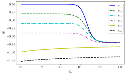
Figure 1: Models of EOS as presented in Eqs. (23a-24b), using the same order, with parameter values chosen to make the curves clear and not overlapping. With the exception of the last two models, all the others exhibit similar properties.

Recent developments [21, 22] demonstrate that the parametrization in Eq. (23b) performs optimally when there is a recent and rapid transition. Remarkably, in Ref. [20] an early-time transition is indistinguishable from a genuine Chevallier-Polarski-Linder parametrization [44, 45] and so, this justifies the reason to focus on fast and recent transitions.

Table 1: Top: Default parameters used in the models. $\Gamma$ is not shown since it is highly dependent on the model. Bottom: Background cosmological parameters. We have approximated the values obtained by [46].

$w_{\rm i}$	$w_{\rm f}$	$z_{\rm t}$	$\Gamma$
$-0.4$	$-1$	$0.5$	$-$
$\Omega_{\rm{m}}$	$\Omega_{\rm{de}}$	$H_{0}$	$z_{\rm{ls}}$
$0.3$	$0.7$	$67$	$1090$

Furthermore, we choose as “default” the values reported in the top part of Tab. 1. We are thus considering mostly freezing models with the exception of Eq. (24b) which is thawing. This choice also allows us to interpret the models as quintessence theories, as the EOS is always above the phantom divide line $w=-1$.

Throughout this paper, we consistently utilize the background parameters listed in the bottom part of Tab. 1.

IV.2 Quintessence potential and field

In view of the above results, we numerically compute the quintessence potential and field for the DE models reported in Sec. IV.1.

To perform numerical integration, it is more convenient to work with the dimensionless quantities $\tilde{\phi}$ and $\tilde{V}$, as defined by Eq. (7). As noted in Sec. II.2, we have the freedom to choose the integration constant, $\tilde{\phi}_{0}$, of the scalar field. For simplicity, we set $\tilde{\phi}(a_{\rm min})=0$, where $a_{\rm min}$ is the lower integration limit.

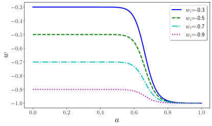
Figure 2: Plot of model $w_{1}$ with $w_{\rm f}=-1$, $\Gamma=10$, $z_{\rm t}=0.5$, showing the EOS for some values of the $w_{\rm i}$ parameter.

In Fig. 2 we report the EOS for the chosen values of the $w_{\rm i}$ parameter. For lower values of $w_{\rm i}$ the transition is more gentle, in the sense that the EOS derivative during the transition is lower. However, the time it takes to transition does not depend on $w_{\rm i}$.

We present the results for the first model, Eq. (23a), with varied $w_{\rm i}$ parameter in Fig. 3. The first observation to do is that as $w_{\rm i}$ approaches $-1$, $\tilde{\phi}$ decreases, resulting in a smaller domain for the potential. In the limit where both $w_{\rm i}$ and $w_{\rm f}$ equal $-1$, the model reduces to the cosmological constant, for which the potential does not depend on $\tilde{\phi}$. Numerically, this degeneracy results in the potential becoming the single point $(\tilde{\phi}_{0},2\Omega_{\rm{de}}^{0})$.

The second observation is that after the transition to $w_{\rm f}=-1$, both the field and the potential become approximately constant. This behaviour is expected since, after the transition, DE behaves as a cosmological constant.

As $w_{\rm i}$ approaches zero, DE tends to a matter-like fluid. For any value of $w_{\rm i}$ inside the interval $(-1,0]$, the potential is divergent in zero. The divergence is faster as $w_{\rm i}$ is closer to zero, while at $w_{\rm i}=0$, $V(a)\approx a^{-3}$, i.e., proportional to the matter density.

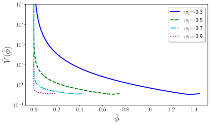
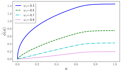
Figure 3: Plots relative to model $w_{1}$ with $w_{\rm f}=-1$, $\Gamma=10$, $z_{\rm t}=0.5$. Top panel: corresponding quintessence potential. The closer is $w_{\rm i}$ to zero, the faster is the divergence of $\tilde{\phi}\rightarrow 0$. Bottom panel: corresponding scalar field. Choosing $w_{\rm i}$ closer to zero results in a steeper slope at early times. It can be shown that for $w_{\rm i}=0$ the field becomes proportional to $\ln(a)$ and thus the slope becomes vertical. After the transition, the field flattens as it enters a slow-rolling period.

The potential and scalar field vary with the $w_{\rm f}$ parameter. The EOS is shown in the top panel of Fig. 4. Since the transition is recent, the potential and the field do not depend as strongly on the $w_{\rm f}$ parameter as they do on the $w_{\rm i}$ parameter, resulting in a narrow cluster of curves. Since $w_{\rm f}\neq-1$ there is no slow-roll phase at late times.

IV.3 Background properties

In this subsection, we describe the evolution of the EOS parameter as a function of the scale factor and for varying values of the free parameters of the model. We also show how the matter density parameter $\Omega_{\rm m}$ is affected.

In the bottom panel of Fig. 4 we present the EOS as we vary the transition speed parameter, $\Gamma$. The model exhibits a spectrum of behaviours, from approximating the $w$CDM with $w=(w_{\rm i}+w_{\rm f})/2$ when $\Gamma=0.1$, to resembling the Heaviside step transition when $\Gamma=10$. The true step transition is also shown and serves as an approximation for fast transition models.

Fig. 5 shows the results obtained varying $\Gamma$. The dependence on this parameter is relatively weak, with only one substantially different curve corresponding to $\Gamma=0.1$. With this choice of parameter, the step-like character of the transition is lost. Apart from this limiting value, the potential and the field do not depend strongly on how fast the transition is. Thus, a true step transition provides a good approximation for fast transition models, and it has the benefit of having analytical $\tilde{V}(a)$ and $\tilde{\phi}(a)$.

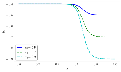
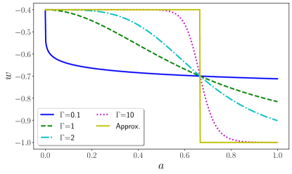
Figure 4: Top panel: EOS of model $w_{1}$ with $w_{\rm i}=-0.4$, $\Gamma=10$, $z_{\rm t}=0.5$ with different values of the $w_{\rm f}$ parameter. Bottom panel: EOS of model $w_{1}$ with $w_{\rm i}=-0.4$, $w_{\rm f}=-1$, $z_{\rm t}=0.5$ with different values of the $\Gamma$ parameter. The yellow line is the Heaviside step function which approximates the model for $\Gamma\rightarrow\infty$. For small values of $\Gamma$, the model tends to a $w$CDM model with $w$ equal to the average of $w_{\rm i}$ and $w_{\rm f}$.

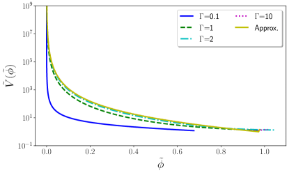
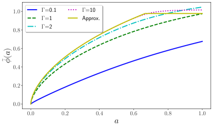
Figure 5: Plots relative to model $w_{1}$ with $w_{\rm i}=-0.4$, $w_{\rm f}=-1$, $z_{\rm t}=0.5$. The yellow line is computed using a true step transition, that in this model corresponds to the limit $\Gamma\rightarrow\infty$. Top panel: corresponding quintessence potential. Bottom panel: corresponding scalar field. Note how much the scalar field flattens after the transition depends on the transition speed. A very fast transition results in $w_{\rm f}=-1$ right after $z_{\rm t}$, while a smoother transition needs additional time to reach the asymptotic value of $w_{\rm f}=-1$, corresponding to the slowly rolling field.

We also analyze the impact of varying $z_{\rm t}$. There are small and distinct growth periods in the potential, that appear during the transition, which can be explained by the smoothness of the transition. For an Heaviside step transition, these growth periods would not be present since the EOS would instantly transition to $-1$, causing the field to abruptly become constant. On the other hand, a smooth transition requires more time to reach the asymptotic value of $w_{\rm f}=-1$, allowing the field to continue evolving for a longer period and resulting in the growth periods observed in the potential function.

The other models we examined, Eqs. (23b-23d), are quite similar to Eq. (23a) as we can choose their parameter values in a way that they can mimic Eq. (23a).

Thus, we shift our attention to the fifth model, Eq. (24a), which is markedly distinct. This functional form contains only two free parameters, $z_{\rm t}$ and $\Gamma$, which influence the final result in a non-trivial manner, making it an intriguing subject. Moreover, all other missing degrees of freedom are completely dependent on these two free parameters, resulting in a restricted range of possible behaviours compared to the other models.

Notably, this model does not exhibit a slow-roll period, since the EOS is always different from $-1$. Additionally, Eq. (24a) cannot be regarded as a fast transition. In fact, while the model starts to behave as a fast transition for large negative values of $\Gamma$, this results in the final value $w(z=0)>-1/3$, that is inadmissible as it would not lead to an accelerated expansion.

Although the parameters influence each other, the scalar field and the potential have a weak dependency on the transition speed and the final value of the EOS, compared to the other parameters. Thus, even if the parameter values depend on each others, the general behaviour is mostly dictated by the parameter $z_{\rm t}$. Eq. (24b) has no free parameters and is classified as a phantom model since it has an EOS $w$ that is smaller than $-1$ and, following the definition of quintessence, it does not look like a genuine quintessence field, but rather as a phantom model. Even though the computation can be put forward even for $w<-1$, it lies beyond the purposes of this paper.

In Fig. 6, we show the effective EOS and the matter density parameter for Eq. (23a). The more $w_{\rm i}$ approaches zero, the more $\Omega_{\rm{m}}$, at early-times ($a\approx 10^{-3}$), differs from unity, even if slightly. In the limit of $w_{\rm i}=0$, at early times $\Omega_{\rm{m}}$ would be equal to $0.3$. This shows how the background affects perturbations and remarks the importance of using the correct exponent for the growth factor in Eq. (13).

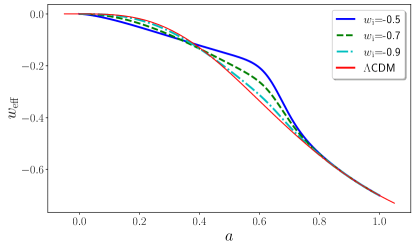
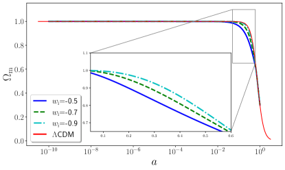
Figure 6: Plots relative to model $w_{1}$ with $w_{\rm f}=-1$, $\Gamma=10$, $z_{\rm t}=0.5$. Top panel: effective forms of EOS. It shows that at early times, DE with $w_{\rm i}$ close to zero has an important impact on the background evolution of the universe. Bottom panel: matter density parameters. Comparing the $w_{\rm i}=-0.5$ to the $\Lambda$CDM curve shows that matter is not completely dominant at last scattering.

Fig. 7 shows the percentage difference between the scaled Hubble function, $E(a)\equiv H(a)/H_{0}$, of the standard cosmological model and the $w$CDM model. The main feature is that the $w$CDM model has an Hubble function always higher than the $\Lambda$CDM model, resulting in an augmented Hubble drag. We therefore expect lower perturbations in the $w$CDM universe.

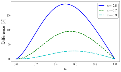
Figure 7: Percentage difference between the $w$CDM and $\Lambda$CDM Hubble functions, defined as $E_{w\rm{CDM}}=E_{\Lambda\rm{CDM}}(1+\%)$. This shows that if the late times acceleration of the universe increases, the Hubble function decreases. Even if we have shown this for the $w$CDM model, it qualitatively holds for fast transition models.

Fig. 8 shows the EOS for Eq. (24a). In the top panel, we can see that at early times, the EOS is consistently close to $-1$, implying that matter dominates. In the bottom panel, instead, we show the effects of varying the parameter $z_{\rm t}$. We can note that the final EOS value and the $\Gamma$ and $z_{\rm t}$ parameters are highly dependent, while the initial value is fixed to $w_{\rm i}=-1$ making this model thawing.

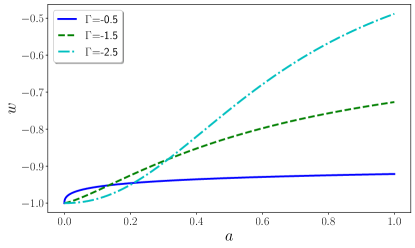
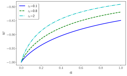
Figure 8: Plots relative to the model with the EOS described by the function $w_{5}$ with $z_{\rm t}=0.5$ for different values of the $\Gamma$ parameter (top panel) and with $\Gamma=-1$ (bottom panel) for different values of the parameter $z_{\rm t}$.

IV.4 Linear regime

In this section, we analyze how the linear matter density contrast is affected by the fast transition models presented in Sec. IV.1.

In this section, we solve the differential equations given by Eq. (15) with initial conditions obtained from the procedure outlined in Sec. III.1, with $a_{\rm min}=a_{\rm{ls}}$. When we include DE perturbations, we assume that the DE EOS is not the same inside or outside the collapsing regions. The difference is encoded in the effective sound speed, that we will fix to $c_{\rm{eff}}=0$ since we lack the underlying model from which the parametrizations emerge. This is the minimum allowed effective sound speed value and it maximizes DE perturbations.

We start by analyzing the first model given by Eq. (23a). Fig. 9 illustrates how linear perturbations depend on the $w_{\rm i}$ parameter in the absence of DE perturbations.

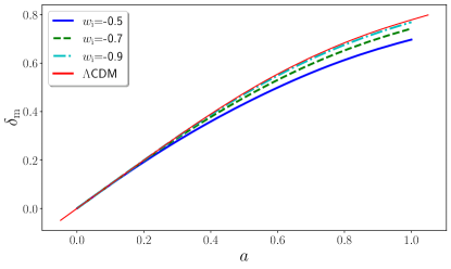
Figure 9: Plot relative to model $w_{1}$ with $w_{\rm f}=-1$, $\Gamma=10$, $z_{\rm t}=0.5$, showing the linear matter density contrast with $\delta_{\rm{de}}=0$. Background quantities are reported in Fig. 6.

Linear perturbations increase as $w_{\rm i}$ decreases, as in this case the model becomes more similar to the $\Lambda$CDM one. In fact, even if lower values of $w$ correspond to higher late-time accelerations, they also correspond to lower Hubble functions for $0<a<1$, as shown in Fig. 7. Due to the Hubble drag, we expect that lower Hubble functions result in higher matter density contrast. Using these considerations, we can explain our results by taking into account the amount of matter at initial conditions. At early times, as there is a small amount of DE, perturbations grow more slowly than in a $\Lambda$CDM model as the rate of expansion is higher in the past. This leads to a smaller value of perturbations today as shown in Fig. 9. We remark that, even though DE perturbations are often neglected in the analysis of perturbations, this is strictly true only for $w_{\rm de}=-1$, as evident also from Eq. (15).

What happens if we include DE perturbations is shown in Fig. 10. When $\delta_{\rm{de}}\neq 0$ the overall behaviour remains qualitatively similar, but with some notable differences. The presence of DE perturbations results in a reduced sensitivity of matter perturbations to the parameters value. Furthermore, if the DE has an EOS with $w_{\rm de}<-1/3$, it tends to dilute matter perturbations, whereas if $w_{\rm de}>-1/3$, it tends to amplify them. This can be deduced by inspecting the source term of Eq. (17). As the transition occurs, DE perturbations cease to grow, and the already present ones gradually decay due to the expansion. As a result, the feedback mechanism weakens, and matter perturbations gradually decouple from DE perturbations.

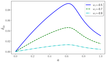
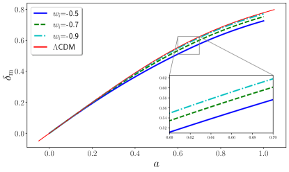
Figure 10: Plots relative to model $w_{1}$ with $w_{\rm f}=-1$, $\Gamma=10$, $z_{\rm t}=0.5$. Top panel: DE perturbations. After the transition, perturbations start to decay since the cosmological constant cannot cluster and the already formed overdensities are diluted by the expansion. Bottom panel: linear matter perturbations with $\delta_{\rm{de}}\neq 0$.

Fig. 11 presents the results obtained by varying the $z_{\rm t}$ parameter. As one could expect, for $z_{\rm t}>2$, the curves become nearly indistinguishable from the $\Lambda$CDM model due to the sub-dominant role of DE at early times. Consequently, an early transition to $w_{\rm f}=-1$ makes the model very similar to the $\Lambda$CDM model. This observation has led us to concentrate on recent transitions and to set $z_{\rm t}=0.5$, while varying the other parameters. On the other hand, if the transition occurs during DE domination, it significantly impacts matter perturbations. We chose the initial EOS value $w_{\rm i}=-0.4$, which is quite distant from $-1$. This choice amplifies the difference between a late-time and an early-time transition. In fact, for a recent transition, this value represents what the EOS had for most of the universe’s evolution, making the difference with the $\Lambda$CDM model even more pronounced.

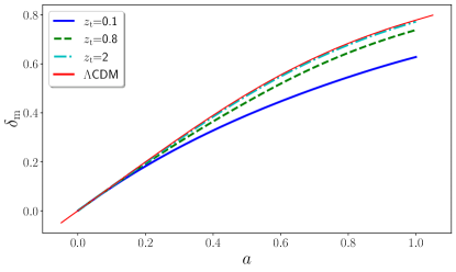
Figure 11: Linear perturbations with $\delta_{\rm{de}}\neq 0$, relative to model $w_{1}$ with $w_{\rm i}=-0.4$, $w_{\rm f}=-1$, $\Gamma=10$. For $z_{\rm t}>2$ the curves become almost indistinguishable from the $\Lambda$CDM model.

In Fig. 12, the results obtained by varying the $\Gamma$ parameter are shown. Even though we have considered a wide range of $\Gamma$ values, leading to significant changes in the EOS, it is evident that the linear perturbations are relatively insensitive to this parameter. Thus, a step transition can approximate a smooth transition quite well at the perturbative level.

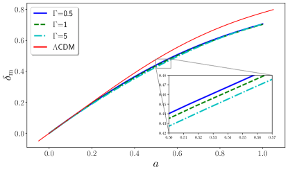
Figure 12: Linear perturbations with $\delta_{\rm{de}}\neq 0$, relative to the model $w_{1}$ with $w_{\rm i}=-0.4$, $w_{\rm f}=-1$, $z_{\rm t}=0.5$. Despite the extreme variations of the EOS, the curves corresponding to the DE model are almost indistinguishable.

Among the six models considered, the first four, Eqs. (23a-23d), behave exactly the same way, as shown in Fig. 13. To ensure a fair comparison, we carefully selected the transition speed parameters to align the models as closely as possible. The maximum deviation between the models is less than $1\%$.

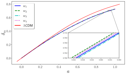
Figure 13: Plot relative to models $w_{1}$, $w_{2}$, $w_{3}$ and $w_{4}$, respectively, with $w_{\rm i}=-0.5$, $w_{\rm f}=-1$, $\Gamma_{1}=10$, $\Gamma_{2}=6.5$, $\Gamma_{3}=0.07$ and $\Gamma_{4}=0.033$. As we can see, the differences between these four models are negligible in the linear regime.

Thus, we now focus on the fifth model Eq. (24a), which has only two parameters: $\Gamma$ and $z_{\rm t}$. These parameters are closely related, as their values determine the rate of the transition as well as the initial and final values of the EOS. We limit our analysis to the non-phantom regime, for which $\Gamma<0$. The results for this model are presented in Fig. 14.

The deviations from the $\Lambda$CDM model are constrained by the requirement that the acceleration parameter is negative today, which implies that $w(a=1)<-1/3$. The plot in Fig. 14 covers almost the full range of admissible $\Gamma$ values. Varying the other free parameter of Eq. (24a), $z_{\rm t}$, yields the linear perturbations shown in Fig. 15.

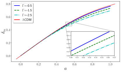
Figure 14: Plot relative to model $w_{5}$ with $z_{\rm t}=0.5$ for linear perturbations with $\delta_{\rm{de}}\neq 0$.

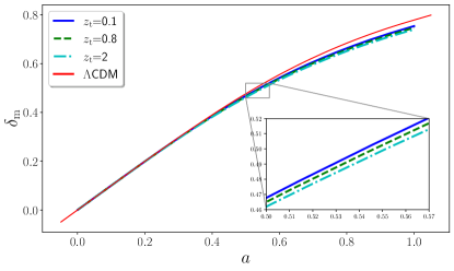
Figure 15: Plots relative to model $w_{5}$ with $\Gamma=-1$ for linear perturbations with $\delta_{\rm{de}}\neq 0$.

The last model, Eq. (24b), has no free parameters and it is entirely in the phantom regime. Thus, as expected, it predicts larger perturbations than in the $\Lambda$CDM model. This happens because the DE component is subdominant until very late in the cosmic history. If we would normalize linear perturbations to be unity today, we would see that the growth factor has lower values than the $\Lambda$CDM model at early times, as structures need to grow more slowly to reach the same speed of the other models today.

IV.5 Nonlinear regime

In this section, we look at nonlinear perturbations when DE is described by the models reported in Sec. IV.1. In particular, we analyze the behaviour of the virialization overdensity and the linearly extrapolated matter density contrast at collapse. The equations to be solved are Eqs. (15) with $c_{\rm{eff}}=0$ for clustering DE and Eq. (9) for smooth models.

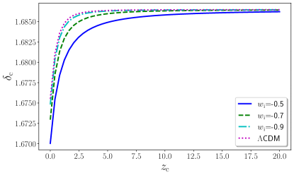
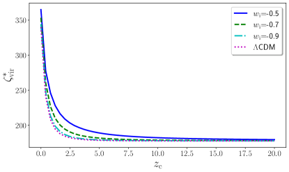
Figure 16: Plot relative to model $w_{1}$ with $w_{\rm f}=-1$, $\Gamma=10$, $z_{\rm t}=0.5$ and $\delta_{\rm{de}}=0$. Top panel: $\delta_{\rm c}$ as a function of the collapse redshift $z_{\rm c}$. Bottom panel: $\zeta_{\rm vir}^{*}$ as a function of the collapse redshift $z_{\rm c}$. The $w_{\rm i}=-0.5$ curve has the highest virialization overdensity.

In Fig. 16 we show the results for nonlinear perturbations with smooth DE. The curves corresponding to $w_{\rm i}=-0.5$ exhibit significant deviation from the $\Lambda$CDM model. This is because, during the evolution of the universe, the EOS, $w_{\rm de}$, had for most of the time the value $-0.5$, which is far from the cosmological constant EOS value. As $w_{\rm i}=-0.5$ is relatively close to zero, DE starts to dominate earlier than models with $w_{\rm i}<-0.5$. Thus, the corresponding curves deviate more from the $\Lambda$CDM case, compared to others.

When examining the virialization overdensity, the curve corresponding to $w_{\rm i}=-0.5$ displays the highest value across all redshifts. This can be attributed to the same effect of the Hubble function that was discussed in the linear perturbation analysis (for more details, see Sec. IV.4). A universe that, at late times, has a faster expansion rate, will exhibit lower values of the Hubble function, as shown in Figs. 7 and 17. Given that the Hubble function dilutes perturbations, overdensities in a universe expanding with a slower rate will face greater dilution while collapsing. Since the collapse time is fixed, to counterbalance the effect of a higher Hubble function, the virialization overdensity will consequently be higher.

In order to understand the increase in the virialization overdensity at late times, it is important to note that the $\zeta^{*}_{\rm{vir}}$ remains constant in the EdS universe. This means that if the Hubble function follows the same evolution as in the EdS universe, the virialization overdensity will remain constant. However, if the Hubble function exceeds that of the EdS universe, the virialization overdensity must increase to counterbalance the Hubble flow that attempts to dilute the perturbation. In Fig. 17, we present the percentage difference between $E_{w\text{CDM}}$ and $E_{\text{EdS}}$. Additionally, in the top panel of Fig. 18, we show the percentage difference between $E_{w\text{CDM}}$ and $E_{\Lambda\text{CDM}}$.

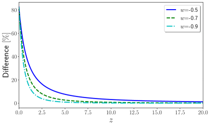
Figure 17: Percentage difference defined by $E_{w\rm{CDM}}(z)=\sqrt{\Omega_{\rm m,0}}E_{\rm{EdS}}(1+\%)$. Note that we scaled the $w$CDM Hubble function $E_{w\rm{CDM}}\rightarrow E_{w\rm{CDM}}/\sqrt{\Omega_{\rm m}}$ in order to make the $w$CDM model reduce to the EdS one at early times.

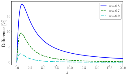
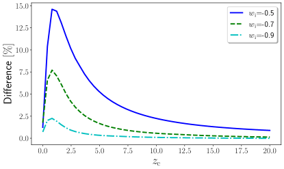
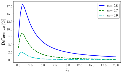
Figure 18: Top panel: percentage difference defined as $E_{w\rm{CDM}}(z)=E_{\Lambda CDM}(z)(1+\%)$. This shows that DE models with $w_{\rm de}>-1$ result in Hubble functions higher than the $\Lambda$CDM model one and thus explain why those models result in higher virialization overdensities than the $\Lambda$CDM model. The maximum point of the ratio approximately corresponds to the time at which the difference between perturbations with DE are most different from the $\Lambda$CDM model. For $w$ close to $-1$, the maximum point is approximately $z_{\rm{max}}\approx 0.6$. Central panel: percentage difference $\zeta_{\rm{de}}^{*}=\zeta_{\Lambda{\rm CDM}}^{*}(1+\%)$ where $\zeta_{\rm{de}}^{*}$ is the virialization overdensity relative to model $w_{1}$ and $\delta_{\rm{de}}\neq 0$. The behaviour is similar to the ratio shown in the top plot. The redshift that maximizes the difference is $z_{\rm{max}}\approx 0.8$. Bottom panel: percentage difference defined by $\zeta_{\rm{de}}^{*}=\zeta_{\Lambda{\rm CDM}}^{*}(1+\%)$, where $\zeta_{\rm{de}}^{*}$ is the virialization overdensity relative to model $w_{1}$ with $\delta_{\rm{de}}=0$. The maximum points are located at respectively $z_{\rm{max}}=[0.4,0.8]$. We can therefore note that the estimate of $z_{\rm{max}}$ obtained from the $w$CDM Hubble function ratio in the top panel is precise within $0.2$ redshift units.

In the central panel of Fig. 18 we can see that for each choice of the parameter, there exists a time interval during which the curves maximally deviates from the $\Lambda$CDM model. In the bottom panel of Fig. 18 we show the percentage difference of $\zeta_{\rm{de}}^{*}$ w.r.t the $\Lambda$CDM one, for the case of smooth DE. As we have pointed out in the linear perturbation analysis, for values of $w$ close to $-1$, allowing DE to cluster or not, does not have appreciable consequences on perturbations. The effect of imposing $\delta_{\rm{de}}=0$ is to enhance the difference between the fast transition model and the $\Lambda$CDM one. The increase in difference depends on the value of the $w_{\rm i}$ parameter. For $w_{\rm i}=-0.5$ the deviation from the $\Lambda$CDM model increases of about $3\%$, while for the other values of $w_{\rm i}$ the difference drops to $1\%$.

We only consider clustering DE in the rest of this section. The results obtained when the $w_{\rm f}$ parameter is changed and DE is allowed to cluster are quite revealing. In the nonlinear regime, perturbations are much more sensitive to the final EOS value, $w_{\rm f}$, compared to the linear perturbations. Small variations in $w_{\rm f}$ can have a dramatic impact on the virialization overdensity and density contrast at $z_{\rm{c}}=0$.

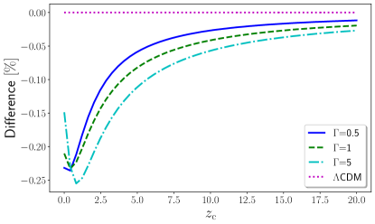
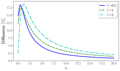
Figure 19: Plots relative to model $w_{1}$ with $w_{\rm i}=-0.4$, $z_{\rm t}=0.5$, $w_{\rm f}=-1$. Top panel: percentage difference of $\delta_{\rm c}$ w.r.t. the $\Lambda$CDM model. Bottom panel: percentage difference of $\zeta^{*}_{\rm{vir}}$ w.r.t. the $\Lambda$CDM model. The redshifts that maximize the differences w.r.t. the $\Lambda$CDM model are $z_{\rm{max}}=[0.4,1.2]$.

The time at which the transition occurs has considerable effects on structure formation only if the transition is recent. Only transitions with $z_{\rm t}\lesssim 2$ are distinguishable from the $\Lambda$CDM paradigm. This is because at early times matter dominates and thus an early-time transition is practically indistinguishable from the $\Lambda$CDM model. Interestingly, the effects are more visible in the approximate range of collapse times $z_{\rm c}\in[0.6,3]$, where we can observe deviations greater than $10\%$. The very recent transition with $z_{\rm t}=0.1$ has the strongest effect, since the transition happened after the DE with $w_{\rm i}=-0.4$ started to dominate.

As one can see in Fig. 19, variations in the $\Gamma$ parameter do not impact significantly the behaviour of the nonlinear perturbations, strengthening the results obtained in Secs. IV.2 and IV.4. Thus, a step transition is a very good approximation to transition models also in the nonlinear regime.

Since the models defined by Eq. (23a), (23b), (23c), and (23d) can be made indistinguishable by appropriately choosing the transition speeds, we do not show results for all of them. The differences between the first four models are shown in Fig. 20. The maximum difference between the corresponding $\delta_{\rm c}$ is less than $0.001\%$, making them completely indistinguishable.

Thus, we shift our attention to the fifth model, Eq. (24a), because it shows interesting differences with the previous ones. The only two free parameters are $\Gamma$ and $z_{\rm t}$. In the other models those parameters are almost independent: for example changing the transition redshift does not affect significantly the transition speed. In this model, the value of one parameter changes the behaviours that should be regulated by the other parameters. Results are shown in Fig. 21. The DE parametrization in question has initial EOS values close to -1, causing matter to remain dominant at later times than the other models, and resulting in all curves converging quickly to the EdS model. We have varied the $\Gamma$ parameter in a range for which the EOS at $a=1$ is always less then $-1/3$.

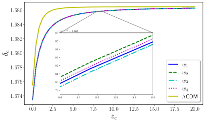
Figure 20: Plot relative to models $w_{1}$, $w_{2}$, $w_{3}$, $w_{4}$ respectively, with $w_{\rm i}=-0.5$, $w_{\rm f}=-1$, $\Gamma_{1}=10$, $\Gamma_{2}=6.5$, $\Gamma_{3}=0.07$, $\Gamma_{4}=0.033$, showing the matter density contrast at collapse. As we can see, the differences between these four models are negligible.

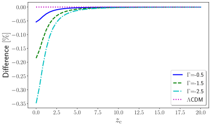
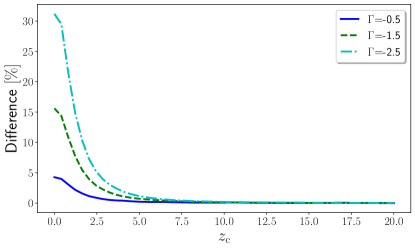
Figure 21: Plots relative to model $w_{5}$ with $z_{\rm t}=0.5$. Top panel: percentage difference of $\delta_{\rm c}$ w.r.t. the $\Lambda$CDM model. Bottom panel: percentage difference of $\zeta^{*}_{\rm{vir}}$ w.r.t. the $\Lambda$CDM model.

A notable difference compared to the previous model, Eq. (23a), is that the redshift which maximizes the difference with respect to the $\Lambda$CDM model is consistently zero, rather than peaking around $z=0.8$. This characteristic remains true independently of the parameter we choose to vary and its value. This is probably due to the fact that this EOS, Eq. (24a), does not behave as a fast transition, but more like a Chevallier-Polarski-Linder parametrization, as one can see in Fig. 14.

In Fig. 22 are shown the results obtained by varying the $z_{\rm t}$ parameter. Since the parameters are strongly intertwined, changing $z_{\rm t}$ also considerably changes the final EOS value and, in the end, the effect on perturbations is quite important.

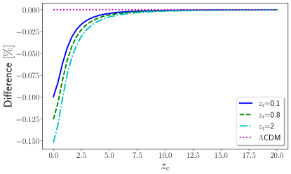
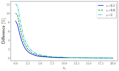
Figure 22: Plots relative to model $w_{5}$ with $\Gamma=-2$. Top panel: percentage difference of $\delta_{\rm c}$ w.r.t. the $\Lambda$CDM model. Bottom panel: percentage difference of $\zeta^{*}_{\rm{vir}}$ w.r.t. the $\Lambda$CDM model.

The last model, Eq. (24b), cannot be analyzed in the same way since it results in $\delta_{\rm{de}}<-1$ that would correspond to a negative energy density. Thus we modified the code to impose $\delta_{\rm{de}}=-1$ when this happens. Results are shown in Fig. 23. This is the only intrinsically phantom model we analyzed and the only case in which the density contrast is greater than the $\Lambda$CDM model one while the virialization overdensity is lower.

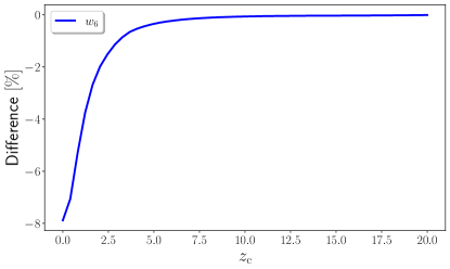
Figure 23: Plot relative to model $w_{6}$. Top panel: percentage difference of $\delta_{\rm c}$ w.r.t. the $\Lambda$CDM model. Bottom panel: percentage difference of $\zeta^{*}_{\rm{vir}}$ w.r.t. the $\Lambda$CDM model. The percentage difference w.r.t. the $\Lambda$CDM model peaks at $z=0$ at about $-8\%$.

IV.6 Matter power spectrum

Given that our primary objective is to compare our results with simulations and observations, we compute the HMF for different fast transition models. Understanding the dependency of the HMF on the DE model is crucial, especially in anticipation of precise measurements in upcoming surveys such as Euclid [27]. The results presented in this section are partially obtained using the CLASS code [48], which is utilized to compute both the linear and nonlinear matter power spectra. The code has been suitably modified to evolve the perturbations for the models considered in this work. Subsequently, we calculate the HMF utilizing the results from Sec. IV.5. In the simulations, we assume a spectral index $n_{\rm s}=0.96$ and use the background parameters provided in Tab. 1. Unless stated otherwise, if $\delta_{\rm{de}}=0$, we also set $c_{\rm{eff}}^{2}=1$. Conversely, if $\delta_{\rm{de}}\neq 0$, we set $c_{\rm{eff}}^{2}=0$. This means that if DE cannot cluster, we set the effective sound speed to unity in the CLASS code. However, if DE can cluster, we maximize its perturbations by setting the sound speed to zero. In Tab. 2 we present the values of $\sigma_{8}(z=0)$ for the model described by Eq. (23a). Allowing DE to cluster consistently increases the $\sigma_{8}$ value, thereby enhancing matter clustering.

Table 2: Present values of $\sigma_{8}$, for model $w_{1}$. The superscript $0$ correspond to $\delta_{\rm{de}}=0$, $c^{2}_{\rm{eff}}=1$, while $1$ to $\delta_{\rm{de}}\neq 0$, $c^{2}_{\rm{eff}}=0$.

$w_{\rm i}$	$-0.5$	$-0.7$	$-0.9$
$\sigma^{0}_{8}$	$0.71$	$0.754$	$0.754$
$\sigma^{1}_{8}$	$0.729$	$0.765$	$0.784$
$w_{\rm f}$	$-0.5$	$-0.7$	$-0.9$
$\sigma^{0}_{8}$	$0.636$	$0.635$	$0.663$
$\sigma^{1}_{8}$	$0.705$	$0.711$	$0.724$
$z_{\rm t}$	$0.1$	$0.8$	$2$
$\sigma^{0}_{8}$	$0.626$	$0.713$	$0.771$
$\sigma^{1}_{8}$	$0.679$	$0.755$	$0.788$
$\Gamma$	$0.5$	$1$	$5$
$\sigma^{0}_{8}$	$0.704$	$0.707$	$0.677$
$\sigma^{1}_{8}$	$0.743$	$0.743$	$0.718$

For freezing models, DE can cluster until the transition occurs, since, according to Eq. (15), only DE with $w\neq-1$ can cluster. This mechanism could result in a decrease of $\sigma_{8}$ by about $8\%$, without significantly impacting the background evolution, for example the maximum deviation of the age of the universe is less then $3\%$.

Fig. 24 presents our results about the linear (top panel) and nonlinear (bottom panel) matter power spectra with the corresponding percentage difference with respect to $\Lambda$CDM for the model described by Eq. (23a) with $\delta_{\rm{de}}=0$.

Note that the positions of the peaks in the ratio are not due to the transition, as altering $z_{\rm t}$ does not shift the peaks. By comparing with Fig. 25, which shows similar results for clustering DE, we note that the local maximum point at low wavenumbers in both the linear and nonlinear spectrum differences is absent. Since this characteristic holds for all the parameters and parameter values, the absence or presence of the low wavenumber peak could be used to differentiate between clustering and smooth DE. Moreover, we can observe that clustering reduces the differences with respect to the standard model, as already seen in other works, such as in Ref. [49].

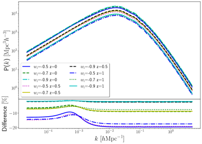
Figure 24: Plots relative to model $w_{1}$ with $w_{\rm f}=-1$, $\Gamma=10$, $z_{\rm t}=0.5$, $\delta_{\rm{de}}=0$. Top panel: linear matter power spectrum. Bottom panel: nonlinear matter power spectrum.

Figure 25: Plots relative to model $w_{1}$ with $w_{\rm f}=-1$, $\Gamma=10$, $z_{\rm t}=0.5$, $\delta_{\rm{de}}\neq 0$. Top panel: linear matter power spectrum. Bottom panel: nonlinear matter power spectrum.

IV.7 The halo mass function

One of the most useful quantities that can be computed in order to test a model is the HMF. This function gives the number of virialised objects with mass $M\in[M,M+\mathrm{d}M]$ per unitary comoving volume, at a given redshift. Calling $n$ the number density of virialised object, the mass function is $\mathrm{d}n/\mathrm{d}M$.

The most consolidate treatment to obtain an analytical expression for the mass function is the Press and Schechter (PS) HMF [50]. To obtain the corresponding expression, we assume that the density field is Gaussian and if $\delta_{M}$ is the density field filtered on a scale $M=4/3\pi R^{3}\bar{\rho}_{m,0}$, then we have

$$p(\delta_{M})=\frac{1}{\sqrt{2\pi}\sigma(M)}e^{\frac{-\delta_{M}^{2}}{2\sigma^{2}(M)}}\,,$$ (25)

where $\sigma(M)$ is the variance of the filtered contrast. Then the probability that the density contrast is larger than a critical value $\delta_{\rm c}$ can be computed as

$$P(\delta_{M}>\delta_{\rm c})=\int_{\delta_{\rm c}}^{\infty}p(\delta_{M})\mathrm{d}\delta_{M}=\mathrm{Erf}\left(\frac{\delta_{M}}{\sqrt{2}\sigma(M)}\right)^{\infty}_{\delta_{\rm c}}\,,$$ (26)

with $\mathrm{Erf}$ the complementary error function. This quantity is approximately proportional to the number of structures with masses larger than $M$. Thus, we have that

$$2\bar{\rho}_{\rm m,0}\frac{\mathrm{d}P(M)}{\mathrm{d}M}=M\frac{\mathrm{d}n}{\mathrm{d}M}\,,$$ (27)

yielding the standard formula

$$\frac{\mathrm{d}n}{\mathrm{d}\ln{M}}=\frac{\bar{\rho}_{0m}}{M}f(\nu)\left|\frac{\mathrm{d\ln{\sigma}}}{\mathrm{d}\ln{M}}\right|\,,$$ (28)

where $\bar{\rho}_{\rm m,0}=\bar{\rho}_{\rm m}(a=1)$. The multiplicity function is $f(\nu)=\sqrt{\frac{2}{\pi}}\nu e^{-\nu^{2}/2}$, with $\nu=\delta_{\rm c}/\sigma$. Usually, the critical value $\delta_{\rm c}$ is taken to be the linearly extrapolated density contrast at collapse as computed in the spherical collapse model, since this value should correspond to fully collapsed objects. The redshift dependence of the HMF comes from both $\delta_{\rm c}(z)$ and the fact that $\sigma(M,z)=D_{+}(z)\sigma(M)$ where $D_{+}(z)$ is the growth factor.

The Sheth–Tormen (ST) [51, 52] HMF extends the PS formalism by assuming that halos are ellipsoidal and not perfectly spherical. The result is that the function $f$ of Eq. (28) changes to

$$f(\nu^{\prime})=\sqrt{\frac{2}{\pi}}A\left[1+\frac{1}{\left(\nu^{\prime}\right)^{2q}}\right]\nu^{\prime}e^{-\left(\nu^{\prime}\right)^{2}/2}\,,$$ (29)

with $\nu^{\prime}=\sqrt{a}\nu$ and fiducial values for the parameters $q=0.3$, $A=0.322$, $a=0.707$, coming from fits of numerical simulations data.

Figure 26: Plots relative to model $w_{1}$ with $w_{\rm f}=-1$, $\Gamma=10$, $z_{\rm t}=0.5$, $\delta_{\rm{de}}=0$. Top panel: ST mass function for various values of $w_{\rm i}$ and redshift. Bottom panel: percentage difference w.r.t the $\Lambda$CDM model defined through the relation $\Lambda$CDM $(1+\%)$.

In Fig. 26, we present the Sheth-Tormen (ST) HMF for smooth DE. For a galaxy of average size, such as the Milky Way, which has a mass of approximately $7\cdot 10^{11}M_{\odot}h^{-1}$, we predict the deviations outlined in Tab. 3. As anticipated from the analysis in Sec. IV.5, we expect the difference with respect to the $\Lambda$CDM model to peak at $z\approx 0.8$. The deviations reported in Tab. 3, even if the considered redshift range is too narrow to draw a definitive conclusion, suggest this behaviour as well for the HMF.

Table 3: Percentage deviations of the ST HMF from the $\Lambda$CDM model, for an average size ($7\cdot 10^{11}M_{\odot}h^{-1}$) galaxy, as extracted from Fig. 26.

$\rm Redshift$	$w_{\rm i}=-0.5$	$w_{\rm i}=-0.7$	$w_{\rm i}=-0.9$
$\,z=0$	$+0.57$	$+0.39$	$+0.14$
$\quad z=0.5$	$-9.7$	$-3.8$	$-1$
$\,z=1$	$-24$	$-10$	$-2.7$

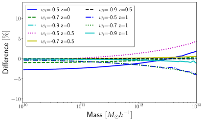
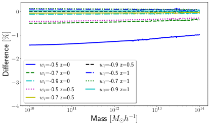
Figure 27: Plots relative to model $w_{1}$ with $w_{\rm f}=-1$, $\Gamma=10$, $z_{\rm t}=0.5$. Top panel: the plot shows $[PS(c_{\rm{s}}=0)/PS(c_{\rm{s}}=1)-1]\times 100$, where the PS functions ratio is used to scale the ST mass function as prescribed by Eq. (30). Bottom panel: percentage difference between the scaled ST mass function and the ST mass function with $c_{\rm{s}}=0$.

The ST formalism offers a possible description of the HMF in clustering DE models. A prescription by [53] implies a rescaling of the ST mass function via the PS mass function [54] according to the following recipe

$$\frac{\mathrm{d}n}{\mathrm{d}\ln{M}}=\frac{\mathrm{d}n_{\rm{ST}}(c_{\rm eff}^{2}=1)}{\mathrm{d}\ln{M}}\frac{\mathrm{d}n_{\rm{PS}}(c_{\rm eff}^{2}=0)/\mathrm{d}\ln{M}}{\mathrm{d}n_{\rm{PS}}(c_{\rm eff}^{2}=1)/\mathrm{d}\ln{M}}\,.$$ (30)

The main idea is that the errors in the PS approach will partially cancel in doing the ratio. As we can see in the top panel of Fig. 27, the effect is greater at higher masses where the recipe tells us that we can expect deviations of about $5\%$ around $M\approx 10^{13}\,M_{\odot}\,h^{-1}$. In the bottom panel of Fig. 27, we show the percentage difference between the scaled mass function computed through Eq. (30) and the ST mass function with clustering DE. In this case the deviations are around $1\%$ and almost constant across the mass range. This confirms that taking the ratio of the PS HMFs partially removes its shortcomings. The top panel in Fig. 27 also shows the difference between clustering and smooth DE on halo formation. With the exception of models with $w_{\rm i}=-0.5$, the difference in the number density of galaxies with average mass, between the clustering and smooth cases, is of the order of $1\%$ which is not particularly significant. Only at higher masses and for higher initial EOS values the effect becomes more significant.

In Fig. 28, we illustrate the HMF, taking into account variations in the final value of the EOS. Note that deviations are expected to increase with redshift up to $z\approx 0.8$. The curves are grouped according to their corresponding redshifts. Despite the high sensitivity of the virialization overdensity to $w_{\rm f}$ variations, the HMF’s sensitivity primarily hinges on redshift rather than the specific value of $w_{\rm f}$. This is anticipated since the HMF is a function of the growth factor, which we showed to be much less sensitive to $w_{\rm f}$ w.r.t. the nonlinear regime. At $z=1$, the curves become indistinguishable due to $z=1$ being prior to both matter-DE equality and the DE transition. Therefore, the deviation between curves clusters with same redshift from the standard model can be attributed to the initial value of the EOS.

In Fig. 29, we display the HMF, adjusting the transition redshift parameter. In this scenario, we anticipate the differences to reach their peak at $z\approx 2$. If the transition is quite recent (as in the case of $z_{\rm t}=0.1$), the model behaves similarly to a $w$CDM with $w=w_{\rm i}=-0.4$, resulting in the maximum difference compared to the $\Lambda$CDM paradigm. However, if the transition to $w_{\rm f}=-1$ occurs before matter-DE equality, the model behaves like the standard one at $z=0$, but shows deviations at higher redshifts.

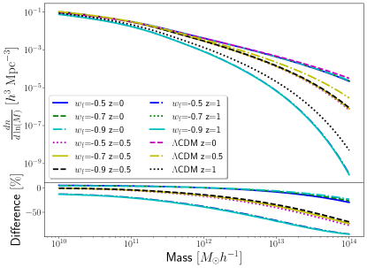
Figure 28: Plots relative to model $w_{1}$ with $w_{\rm i}=-0.4$, $\Gamma=10$, $z_{\rm t}=0.5$, $\delta_{\rm{de}}\neq 0$. Top panel: ST mass function for various values of $w_{\rm f}$ and redshift. Bottom panel: Percentage difference w.r.t. the $\Lambda$CDM model defined through the relation $\Lambda$CDM $(1+\%)$.

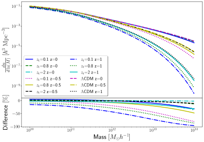
Figure 29: Model $w_{1}$ with $w_{\rm i}=-0.4$, $w_{\rm f}=-1$, $\Gamma=10$, $\delta_{\rm{de}}\neq 0$ for several values of $z_{\rm t}$.

In Fig. 30 the results for the HMF when the transition speed is varied are shown. The effects of the transition speed on galaxy formation are quite low at $z=0$: the differences between the curves are $\approx 0.1\%$ for an average mass galaxy. The differences become more prominent at higher redshifts: curves with $z=1$ can differ by $22\%$, while at $z=0.5$ can differ by $6\%$. Those differences at high redshifts are amplified by the choice $w_{\rm i}=-0.4$. An initial value closer to $-1$ dampens those differences. Despite that, only measurements at $z\gtrapprox 0.5$ could possibly detect the transition speed effects.

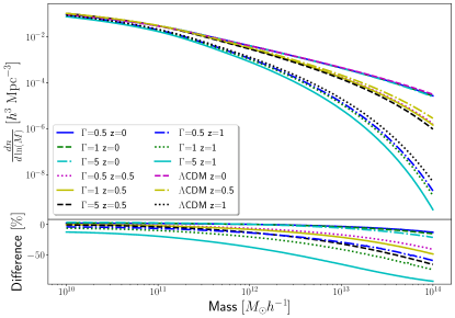
Figure 30: Plot relative to model $w_{1}$ with $w_{\rm i}=-0.4$, $w_{\rm f}=-1$, $z_{\rm t}=0.5$, $\delta_{\rm{de}}\neq 0$ for various values of $\Gamma$ and redshift.

The final model we examine is Eq. (24a) and depicted in Fig. 32. This model is unique due to its initial value of the EOS being fixed at $-1$, leading to a thawing behaviour. Because of the initial condition $w_{i}=-1$, the curves do not cluster in groups with the same redshift, and the range of variation is narrower. For $\Gamma=-0.5$, the EOS is bounded between $-1$ and $-0.9$. For lower values (e.g., $\Gamma=-2.5$), the model shows a slow transition from $-1$ to $-0.5$. Focusing on the model with $\Gamma=-2.5$, we observe that at $z=0$, the model predicts a $30\%$ increase in massive galaxies, and at $z=0.5$, it predicts a $20\%$ decrease. Thus, from $z=0.5$ to $z=0$, the number of massive galaxies increases by $50\%$. This suggests a recent and brief period during which many smaller galaxies rapidly merged to form more massive ones. However, it is important to note that this effect is present in all the other models as well, with the difference being that the other models generally predict a lower number of massive galaxies than the $\Lambda$CDM model. This effect is particularly notable for this model since it predicts a higher number of massive galaxies compared to the standard model.

Regarding the other models, they bear a strong resemblance to the model of Eq. (23a). The main differences lie in the exact shape of the transition. As we have seen here and in previous sections, structure formation is quite insensitive to the exact form of the transition, thus reporting them would not add more insights on the physics. We just show in Fig. 31 the HMF for the first four models, with fixed parameter values and different redshifts. The maximum deviations at redshift $z=1$ are $<5\%$ at high masses and $<0.5\%$ for an average mass galaxy.

Figure 31: Comparison of the HMFs for model $w_{1}$, $w_{2}$, $w_{3}$, $w_{4}$ with $w_{\rm i}=-0.5$, $w_{\rm f}=-1$, $z_{\rm t}=0.5$, $\Gamma_{1}=10$, $\Gamma_{2}=6.5$, $\Gamma_{3}=0.07$, $\Gamma_{4}=0.033$. The models are indistinguishable.

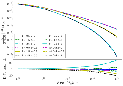
Figure 32: Plot relative to model $w_{5}$ with $z_{\rm t}=0.5$, $\delta_{\rm{de}}\neq 0$. Top panel: ST mass function for various values of $\Gamma$ and redshift. Bottom panel: Percentage difference w.r.t. the $\Lambda$CDM model defined through the relation $\Lambda$CDM $(1+\%)$.

V Outlooks and perspectives

In this study, we analyzed six fast transition DE models. Five of them are argued as effective quintessence fluids while all lie within the category of effective Horndeski fluids, i.e., these scenarios originally emerged from exploring the Horndeski parameter space. For those frameworks allowing a quintessence interpretation, we computed the quintessence field and potential. Our results are summarized below.

• The field potential exhibits a weak dependence on both the final value and the transition speed of the EOS. Notably, the dependence on the transition speed is particularly weak and we demonstrated that a Heaviside step transition can serve as a good approximation for fast transition models, with the benefit of having analytical $g(a)$ and $V(a)$.

We computed the effects of such models on the expansion history of the universe and on structure formation. The performed analysis brought to light the most important aspects of the fast transition models. In the simplest analysis of the matter linear perturbations we found results consistent to the scalar field analysis.

• Also linear matter perturbations are quite insensitive to the transition speed, suggesting that a Heaviside step transition can approximate well fast transition models also at perturbative level.

• For all the non-phantom models we found that they result in lower density contrast respect to the standard model. We showed that this can be understood with the background evolution, by comparing the Hubble functions of the different models with the $\Lambda$CDM one.

• Linear perturbations are insensitive to the redshift at which the transition happens ($z_{\rm t}$) if $z_{\rm t}\gtrapprox 2$. This is due to the fact that matter-DE equality happens between $z=1$ and $z=0.3$. If the transition happens before matter-DE equality, when DE is sub-dominant, DE effects are not evident. On the other hand if the transition happens within DE domination, the effects are more pronounced.

• We compared the case of $\delta_{\rm{de}}=0$ to $\delta_{\rm{de}}\neq 0$ and found that when DE perturbations are included, the overall behaviour remains qualitatively similar. The presence of DE perturbations results in damping of matter perturbations due to the interactions between the two fluids. If DE has $w_{\rm de}<-1/3$, it tends to dilute matter perturbations, whereas if $w_{\rm de}>-1/3$, it tends to amplify them.

• The models $w_{1}$, $w_{2}$, $w_{3}$ and $w_{4}$ are indistinguishable one from the other, because the maximum difference between them is less then $1\%$. The $w_{6}$ model, being phantom, results in perturbations higher than the standard model.

We also analyzed matter perturbations in the nonlinear regime. We computed the virialization overdensity, $\zeta^{*}_{\rm{vir}}$, and the linearly extrapolated matter density contrast at collapse, $\delta_{\rm c}$. The latter quantity is very significant as we used it to compute the HMF.

• We understood in a simple way the qualitative behaviour of the virialization overdensity and its main features, such as the presence of a peak in the percentage difference w.r.t. the $\Lambda$CDM one and its position. In fact, we explained why the ratio between the Hubble function for a $w$CDM universe to the standard model one, shows the same qualitative behaviour as the ratio of the virialization overdensities. We computed the location of the peak using the Hubble functions and obtained, for $w\rightarrow-1$, $z\approx 0.6$.

• The peaks in the virialization ratios are generally located at $z=0.4\pm 0.2$ and $z=0.8\pm 0.2$ which average at $z=0.6\pm 0.2$, i.e., very close to the transition redshift constraints [55, 56, 57], while far from the equivalence DE-dark matter [58]. The Hubble function approximation does not work well in predicting the peaks when $z_{\rm t}$ parameter is varied. In the case of $z_{\rm t}=2$ we found the peak at $z=2.9\pm 0.2$.

• We showed how the shape of the virialization overdensity can be understood by comparing the model’s Hubble function to the EdS one.

• By varying the transition speed we found that also nonlinear perturbations are quite insensitive to the parameter, confirming again the previous results.

• In the nonlinear regime, perturbations exhibit high sensitivity to the final EOS value in comparison to the linear regime. This is because in the nonlinear phase, the changes happen much faster and thus even if DE has a short time, after the transition, in which it can act, the effects are quite large.

• We compared the clustering case, $\delta_{\rm{de}}\neq 0$, to the smooth case, $\delta_{\rm{de}}=0$. The main effect of DE perturbations is to dampen, on average, by $2\%$ the differences of the model w.r.t. the $\Lambda$CDM model. The dampening depends on the exact parameter value considered.

• Consistently with the linear results, the models $w_{1}$, $w_{2}$, $w_{3}$ and $w_{4}$ are indistinguishable one from the other.

We then analyzed statistical properties of the matter clustering, namely the linear and nonlinear power spectrum and the HMF. We found that:

• Freezing fast transition models can lower the present $\sigma_{8}$ value by around $8\%$, without affecting too much the background evolution. This suggest that it may be possible to relieve the $\sigma_{8}$ tension with such models. This possibility deserves a thorough investigation, and we intend to pursue it in a future work.

• By comparing the matter power spectrum for smooth and clustering DE we found that a peak at low wavenumbers, present in the smooth case, vanishes in the clustering case. This effect could be used to detect signatures of clustering DE.

• Since perturbations are maximally different from the standard model at $z\approx 0.6$, we argue that this happens also for the HMF. The redshift range we have used is too narrow to prove this; thus, we plan to extend it in future work.

• We showed that the differences between the HMF in the clustering and smooth case are small $\approx 1\%$ for average size galaxies, while they can become more important $\approx 5\%$ for massive galaxies.

• We explained why the HMF shows a weak dependency on $w_{\rm f}$. The dependency of the HMF on the $z_{\rm t}$ parameter is very weak for $z_{\rm t}\gtrapprox 2$. For $z_{\rm t}=2$ at $z=0$, the model is indistinguishable from the standard one, while there are some signs of the transition at higher redshifts $z=0.5,1$.

• All the models predict a lower concentration of massive galaxies, except Eq. (24a) which is thawing, and predicts higher numbers of massive galaxies w.r.t. the $\Lambda$CDM model at $z=0$. This model with $\Gamma=-2.5$, predicts that from $z=0.5$ to $z=0$, the number of massive galaxies increases by $50\%$ w.r.t. the $\Lambda$CDM scenario, implying a period of fast galaxy merging which may be detectable. This is a common feature of the models: they predict a merging rate higher then in the $\Lambda$CDM universe.

We conclude by presenting perspectives and research challenges below.

• Can an evolving fast-transition DE influence gravitational lensing, and how? By changing the EOS of DE to a fast-transition model, we can study how a sudden period in which DE undergoes a transition affect this observable.

• Determining whether freezing fast transition models can alleviate the $\sigma_{8}$ tension and to clarify their impact on the Hubble tension. Indeed, the presence of DE perturbations may influence baryon acoustic oscillations and the cosmic microwave background power spectrum. A dynamical DE also changes the expansion history of the universe and thus the relation between the values of the Hubble parameter at different redshifts. Thus, we will explore the possibility of a model that can alleviate both tension at the same time.

• Investigating whether future data from the Euclid mission will be accurate enough to discern differences in the nonlinear power spectrum between clustering and smooth DE cases.

References

- [1] Brian P. Schmidt et al. The High Z supernova search: Measuring cosmic deceleration and global curvature of the universe using type Ia supernovae. Astrophys. J., 507:46–63, 1998.
- [2] S. Perlmutter et al. Measurements of and from 42 high redshift supernovae. Astrophys. J., 517:565–586, 1999.
- [3] Adam G. Riess et al. Type Ia supernova discoveries at z 1 from the Hubble Space Telescope: Evidence for past deceleration and constraints on dark energy evolution. Astrophys. J., 607:665–687, 2004.
- [4] Jerome Martin. Everything You Always Wanted To Know About The Cosmological Constant Problem (But Were Afraid To Ask). Comptes Rendus Physique, 13:566–665, 2012.
- [5] Orlando Luongo and Marco Muccino. Speeding up the universe using dust with pressure. Phys. Rev. D, 98(10):103520, 2018.
- [6] Lamartine Liberato and Rogerio Rosenfeld. Dark energy parameterizations and their effect on dark halos. JCAP, 07:009, 2006.
- [7] M. Muccino, L. Izzo, O. Luongo, K. Boshkayev, L. Amati, M. Della Valle, G. B. Pisani, and E. Zaninoni. Tracing dark energy history with gamma ray bursts. Astrophys. J., 908(2):181, 2021.
- [8] Salvatore Capozziello, Rocco D’Agostino, and Orlando Luongo. Thermodynamic parametrization of dark energy. Phys. Dark Univ., 36:101045, 2022.
- [9] Orlando Luongo and Marco Muccino. Kinematic constraints beyond using calibrated GRB correlations. Astron. Astrophys., 641:A174, 2020.
- [10] Alejandro Aviles, Jaime Klapp, and Orlando Luongo. Toward unbiased estimations of the statefinder parameters. Phys. Dark Univ., 17:25–37, 2017.
- [11] Alejandro Aviles, Christine Gruber, Orlando Luongo, and Hernando Quevedo. Cosmography and constraints on the equation of state of the Universe in various parametrizations. Phys. Rev. D, 86:123516, 2012.
- [12] Salvatore Capozziello, Rocco D’Agostino, and Orlando Luongo. Extended Gravity Cosmography. Int. J. Mod. Phys. D, 28(10):1930016, 2019.
- [13] Salvatore Capozziello and Mariafelicia De Laurentis. Extended Theories of Gravity. Phys. Rept., 509:167–321, 2011.
- [14] Victor I. Afonso, Gonzalo J. Olmo, Emanuele Orazi, and Diego Rubiera-Garcia. Correspondence between modified gravity and general relativity with scalar fields. Phys. Rev. D, 99(4):044040, 2019.
- [15] Tsutomu Kobayashi. Horndeski theory and beyond: a review. Rept. Prog. Phys., 82(8):086901, 2019.
- [16] Richard A. Battye and Francesco Pace. Approximation of the potential in scalar field dark energy models. Phys. Rev. D, 94(6):063513, 2016.
- [17] Orlando Luongo, Giovanni Battista Pisani, and Antonio Troisi. Cosmological degeneracy versus cosmography: a cosmographic dark energy model. Int. J. Mod. Phys. D, 26(03):1750015, 2016.
- [18] Orlando Luongo and Marco Muccino. Intermediate redshift calibration of gamma-ray bursts and cosmic constraints in non-flat cosmology. Mon. Not. Roy. Astron. Soc., 518(2):2247–2255, 2022.
- [19] Orlando Luongo and Marco Muccino. A Roadmap to Gamma-Ray Bursts: New Developments and Applications to Cosmology. Galaxies, 9(4):77, 2021.
- [20] Sebastian Linden and Jean-Marc Virey. A test of the CPL parameterization for rapid dark energy equation of state transitions. Phys. Rev. D, 78:023526, 2008.
- [21] Mariana Jaber and Axel de la Macorra. Constraints on Steep Equation of State for the Dark Energy using BAO. 4 2016.
- [22] Bruce A. Bassett, Martin Kunz, Joseph Silk, and Carlo Ungarelli. A Late time transition in the cosmic dark energy? Mon. Not. Roy. Astron. Soc., 336:1217–1222, 2002.
- [23] Xiaolei Li and Arman Shafieloo. Evidence for Emergent Dark Energy. Astrophys. J., 902(1):58, 2020.
- [24] Xiaolei Li and Arman Shafieloo. A Simple Phenomenological Emergent Dark Energy Model can Resolve the Hubble Tension. Astrophys. J. Lett., 883(1):L3, 2019.
- [25] J. A. S. Lima, V. Zanchin, and Robert H. Brandenberger. On the Newtonian cosmology equations with pressure. Mon. Not. Roy. Astron. Soc., 291:L1–L4, 1997.
- [26] L. R. Abramo, R. C. Batista, L. Liberato, and R. Rosenfeld. Structure formation in the presence of dark energy perturbations. JCAP, 11:012, 2007.
- [27] Tiago Castro, Valerio Marra, and Miguel Quartin. Constraining the halo mass function with observations. Mon. Not. Roy. Astron. Soc., 463(2):1666–1677, 2016.
- [28] Alessio Belfiglio, Roberto Giambò, and Orlando Luongo. Alleviating the cosmological constant problem from particle production. Class. Quant. Grav., 40(10):105004, 2023.
- [29] Alessio Belfiglio, Youri Carloni, and Orlando Luongo. Particle production from non-minimal coupling in a symmetry breaking potential transporting vacuum energy. 7 2023.
- [30] Orlando Luongo and Tommaso Mengoni. Quasi-quintessence inflation with non-minimal coupling to curvature in the Jordan and Einstein frames. 9 2023.
- [31] Alberto Navarro and Jose Navarro. Lovelock’s theorem revisited. J. Geom. Phys., 61:1950–1956, 2011.
- [32] Tsutomu Kobayashi. Horndeski theory and beyond: a review. Rept. Prog. Phys., 82(8):086901, 2019.
- [33] Ryotaro Kase and Shinji Tsujikawa. Dark energy in horndeski theories after gw170817: A review. International Journal of Modern Physics D, 28(05):1942005, 2019.
- [34] Christos Charmousis, Edmund J. Copeland, Antonio Padilla, and Paul M. Saffin. General second order scalar-tensor theory, self tuning, and the Fab Four. Phys. Rev. Lett., 108:051101, 2012.
- [35] F. Pace, J. C. Waizmann, and M. Bartelmann. Spherical collapse model in dark-energy cosmologies. mnras, 406(3):1865–1874, August 2010.
- [36] Francesco Pace, Robert Reischke, Sven Meyer, and Björn Malte Schäfer. Effects of tidal gravitational fields in clustering dark energy models. Mon. Not. Roy. Astron. Soc., 466(2):1839–1847, 2017.
- [37] Sophia Haude, Shabnam Salehi, Sofía Vidal, Matteo Maturi, and Matthias Bartelmann. Model-Independent Determination of the Cosmic Growth Factor. 12 2019.
- [38] Francesco Pace, Sven Meyer, and Matthias Bartelmann. On the implementation of the spherical collapse model for dark energy models. JCAP, 10:040, 2017.
- [39] Li-Min Wang and Paul J. Steinhardt. Cluster abundance constraints on quintessence models. Astrophys. J., 508:483–490, 1998.
- [40] Anto I. Lonappan, Sumit Kumar, Ruchika, Bikash R. Dinda, and Anjan A. Sen. Bayesian evidences for dark energy models in light of current observational data. Phys. Rev. D, 97(4):043524, 2018.
- [41] Gong-Bo Zhao, Robert G Crittenden, Levon Pogosian, and Xinmin Zhang. Examining the evidence for dynamical dark energy. Physical Review Letters, 109(17):171301, 2012.
- [42] Xuheng Ding, Marek Biesiada, Shuo Cao, Zhengxiang Li, and Zong-Hong Zhu. Is there evidence for dark energy evolution? Astrophys. J. Lett., 803(2):L22, 2015.
- [43] Varun Sahni, Arman Shafieloo, and Alexei A. Starobinsky. Model independent evidence for dark energy evolution from Baryon Acoustic Oscillations. Astrophys. J. Lett., 793(2):L40, 2014.
- [44] Michel Chevallier and David Polarski. Accelerating universes with scaling dark matter. Int. J. Mod. Phys. D, 10:213–224, 2001.
- [45] Eric V. Linder. Exploring the expansion history of the universe. Phys. Rev. Lett., 90:091301, 2003.
- [46] N. Aghanim et al. Planck 2018 results. VI. Cosmological parameters. Astron. Astrophys., 641:A6, 2020. [Erratum: Astron.Astrophys. 652, C4 (2021)].
- [47] Rocco D’Agostino, Orlando Luongo, and Marco Muccino. Healing the cosmological constant problem during inflation through a unified quasi-quintessence matter field. Class. Quant. Grav., 39(19):195014, 2022.
- [48] Diego Blas, Julien Lesgourgues, and Thomas Tram. The cosmic linear anisotropy solving system (class). part ii: approximation schemes. Journal of Cosmology and Astroparticle Physics, 2011(07):034–034, 2011.
- [49] R. C. Batista and F. Pace. Structure formation in inhomogeneous Early Dark Energy models. JCAP, 06:044, 2013.
- [50] William H. Press and Paul Schechter. Formation of Galaxies and Clusters of Galaxies by Self-Similar Gravitational Condensation. Astrophys. J., 187:425–438, February 1974.
- [51] Ravi K. Sheth and Giuseppe Tormen. Large scale bias and the peak background split. Mon. Not. Roy. Astron. Soc., 308:119, 1999.
- [52] Ravi K. Sheth, H. J. Mo, and Giuseppe Tormen. Ellipsoidal collapse and an improved model for the number and spatial distribution of dark matter haloes. Mon. Not. Roy. Astron. Soc., 323:1, 2001.
- [53] Paolo Creminelli, Guido D’Amico, Jorge Norena, Leonardo Senatore, and Filippo Vernizzi. Spherical collapse in quintessence models with zero speed of sound. JCAP, 03:027, 2010.
- [54] William H. Press and Paul Schechter. Formation of galaxies and clusters of galaxies by selfsimilar gravitational condensation. Astrophys. J., 187:425–438, 1974.
- [55] Salvatore Capozziello, Omer Farooq, Orlando Luongo, and Bharat Ratra. Cosmographic bounds on the cosmological deceleration-acceleration transition redshift in gravity. Phys. Rev. D, 90(4):044016, 2014.
- [56] Salvatore Capozziello, Peter K. S. Dunsby, and Orlando Luongo. Model-independent reconstruction of cosmological accelerated–decelerated phase. Mon. Not. Roy. Astron. Soc., 509(4):5399–5415, 2021.
- [57] Marco Muccino, Orlando Luongo, and Deepak Jain. Constraints on the transition redshift from the calibrated gamma-ray burst Ep–Eiso correlation. Mon. Not. Roy. Astron. Soc., 523(4):4938–4948, 2023.
- [58] Anna Chiara Alfano, Carlo Cafaro, Salvatore Capozziello, and Orlando Luongo. Dark energy-matter equivalence by the evolution of cosmic equation of state. Physics of the Dark Universe, 42:101298, December 2023.