Learning to Optimize: Accelerating Optimal Power Flow via Data-driven Constraint Screening

Abstract

This paper introduces a novel data-driven constraint screening approach aimed at accelerating the solution of convexified optimal power flow (OPF) by eliminating constraints that are non-binding at the optimum. Our constraint screening process leverages an input-convex neural network, trained to predict optimal dual variables based on problem parameters. The results demonstrate that, subject to certain mild conditions on the OPF model, our proposed method guarantees an identical solution to the full OPF but significantly reduces computational time. Extensive simulations conducted on the OPF based on the convexified DistFlow model demonstrate that our method outperforms other constraint screening techniques.

I Introduction

The Optimal Power Flow (OPF) is an optimization problem that determines the optimal settings for control variables in an electric power network. Its primary goal is to minimize the total generation cost while satisfying various operational constraints (e.g., generation limits, voltage limits, and line capacity limits). The increasing integration of distributed energy resources (DERs) leads to an increased demand for more frequent OPF solutions. In addition, efficient solutions are increasingly essential as OPF requires resolution across a wide range of scenarios.

AC Optimal Power Flow (ACOPF) accurately represents power network physics. However, it is inherently nonconvex due to a series of nonlinear equality constraints (AC power flow equations). The non-convexity poses a challenge for optimization solvers to find a globally optimal solution, which often necessitates the acceptance of locally optimal solutions [1]. To address this issue, various linearization and convexification techniques have been proposed for ACOPF. Those approximations substitute the nonconvex constraints with linear or convex ones, resulting in what we hereafter refer to as ‘convexified OPF’ (C-OPF). The solutions obtained through C-OPF possess an advantageous characteristic: any solution found locally is guaranteed to be globally optimal.

Assuming fixed voltage magnitudes, minimal voltage angle variations, and negligible line resistances, DCOPF approximates AC power flow by using a series of linear equations; see e.g., [2]. The DistFlow equations represent power flow using both line and nodal variables [3]. Extensive research has been conducted on OPF utilizing second-order cone relaxation of DistFlow equations, henceforth called socp-dOPF [4, 5, 6]. Under certain conditions for radial networks, ACOPF solutions can be recovered from the solution of socp-dOPF [7, 6]. For more general networks, ACOPF may be relaxed to a semidefinite program [8, 9, 10]. Other relaxations of ACOPF include quadratic convex relaxation [11], McCormick relaxation [12], and chordal decomposition [13], all of which employ second-order cone and/or semidefinite constraints. A comprehensive review of convex approximations and relaxations to ACOPF is provided in [14].

In this paper, we aim to improve the computational performance of OPF solvers, irrespective of the underlying optimization algorithm, by introducing a machine learning-based technique called Constraint Screening (CS). CS identifies and eliminates non-binding constraints, reducing problem size and accelerating solving times.

I-A Prior Work

Earliest works on the removal of redundant and non-binding constraints are for linear programs [15, 16]. Recent domain-specific CS methods for power systems are based on geometry of the feasible set or machine learning techniques.

CS methods based on feasible set geometry analyze the constraints a priori to generate a list of constraints which are provably non-binding at the optimum. In this category, [17], [18], [19] propose algorithms to eliminate redundant line flow constraints for various formulations of DCOPF, based on solving an auxiliary optimization problem per constraint. CS has also been utilized for unit commitment. Madani et al. [20] use a low-order model to eliminate constraints and generate cuts for branch-and-bound. Pineda et al. [21], Zhang et al. [22], and Porras et al. [23] develop methods to accelerate branch-and-bound by eliminating network constraints.

CS methods based on machine learning use historical or synthetic OPF datasets to train different models. Typically, the inputs of those models are load demand while the outputs contain the set of binding constraints at the optimum, or optimal decision variables. For example, Deka & Misra [24] and Hasan & Kargarian [25] train a deep neural network (DNN) based classifiers to learn the mapping between problem parameters and the binding constraints. Alternatively, we can learn the mapping between problem parameters and optimal dual variables, which subsequently can assist in identifying the status of each constraint. Dual variables play a pivotal role in DNN applications for OPF [26, 27, 28]. To the best of our knowledge, [29] is the only work that has explored DNN-based learning for dual variables. Notably, their work is limited to DCOPF, whereas our contributions extend the framework to cover any arbitrary C-OPF.

I-B Contribution

In this paper, we propose a CS method to reduce the size of C-OPF problems. We first represent C-OPF as a parameterized convex optimization problem with parameters representing values such as load demands, generation bounds, voltage bounds, line flow limits, etc. The proposed method uses a specific class of DNNs called input-convex neural networks (ICNNs) to learn the mapping from parameters to optimal dual variables. Once trained, ICNN can predict optimal dual variables for parameters representing new C-OPF instances, which are used to infer non-binding constraints via the Karush-Kuhn-Tucker (KKT) conditions. Removal of non-binding constraints provides a much smaller problem that can be solved much faster. Furthermore, we tackle the challenge of misclassified constraints that arise due to inaccuracies in predicting optimal dual variables. Our proposed approach incorporates a recovery stage, where any identified violated constraints following the solution of the reduced C-OPF are retrospectively added to the list of active constraints, and the problem is resolved. We show that the convexity of C-OPF ensures that even in the worst case of mispredicted constraints, only one iteration of re-solving is required.

Our work builds on the data-driven DCOPF solver [29], but improves upon it in significant ways. First, our framework can handle nonlinear convex constraints, whereas [29] was restricted to linear DCOPF. Dealing with nonlinear convex constraints requires further examination of the existence and uniqueness of dual variables, as well as the validity of using dual variables for constraint classification. We furnish the necessary analysis in this regard. Second, the method in [29] is not robust to mispredictions of dual variables, an issue we address in this work. Last, we develop a novel data augmentation technique to expedite the generation of synthetic data for training the ICNN.

The main contributions of this work are summarized as follows.

• We propose a CS method for accelerating C-OPF solvers, which leverages ICNNs to learn the mapping from problem parameters to the optimal dual variables. Predicted dual variables are used to classify non-binding constraints. If mispredictions are detected, C-OPF is resolved with an augmented list of constraints.

• We establish a model-agnostic condition for generic C-OPF to verify whether strong duality holds over a given set of parameters. Strong duality is essential for using dual variables to classify constraints at the optimum. The condition is verified as being valid for socp-dOPF.

• We provide an efficient method to generate datasets for the ICNN, which exploits the convexity of C-OPF. Our method is shown to be more efficient than random sampling in the space of problem parameters.

I-C Organization and Notation

The paper is structured as follows. Section II introduces a standard form of C-OPF that encompasses various OPF models, using socp-dOPF as a specific example. Section III is bifurcated into two parts: the first part outlines a mild condition under which the proposed CS method is applicable to a given C-OPF model, while the second part details the algorithms for training the ICNN and leveraging it to expedite C-OPF, accompanied by corresponding analyses. Section IV conducts simulations to comparatively analyze the proposed CS method against other methods for accelerating C-OPF. The conclusion of the paper is presented in Section V, accompanied by all the proofs provided in the Appendix.

The set of real numbers is symbolized by . Matrices and vectors are depicted in bold typeface. Uppercase calligraphic characters are used to represent sets. $[n]$ and $[n]_{0}$ denote the sets $\{1,\dots,n\}$ and $\{0,\dots,n\}$ respectively. For a vector $\mathbf{a}\in n$, $\mathbf{a}_{i}$ is its ${i}^{\text{th}}$ element while $[\mathbf{a}]_{\mathcal{S}}$ denotes the subvector of $\mathbf{a}$ corresponding to a set $\mathcal{S}\subseteq[n]$. $\mathbf{a}\preceq\mathbf{b}$ denotes that $\mathbf{a}$ is elementwise lesser than or equal to $\mathbf{b}$. For a vector-valued function $f(\cdot)$, $\nabla_{\mathbf{x}}f(\mathbf{x})$ is the transpose of the Jacobian matrix. $|\mathcal{S}|$ denotes the cardinality of a finite set $\mathcal{S}$.

II C-OPF as Parameterized Convex Optimization

In this section, we represent C-OPF as a parameterized convex optimization problem. This allows us to generate a well-defined mapping between problem parameters and optimal dual variables, which can then be used for CS. In general, constraints for any OPF problem can broadly be categorized into two types: the power flow equations and other operational constraints. The power flow model is usually fixed and does not vary from one problem instance to another. On the other hand, the operational constraints are meant to restrict decision variables such as power injections, line flows, and nodal voltages within ranges that ensure satisfactory operation of the power network. The bounds describing the operational constraints serve as problem parameters in our formulation. Concretely, we represent any C-OPF model as the following parameterized problem.

$$\mathcal{J}(\boldsymbol{\gamma},\boldsymbol{\xi})\stackrel{{\scriptstyle\Delta}}{{=}}\inf\limits_{\mathbf{x}}\quad f(\mathbf{x})$$ (1)

s.t. $$g(\mathbf{x})\preceq\mathbf{0},\quad h(\mathbf{x})=\mathbf{0},$$ (2)

$$\tilde{g}(\mathbf{x})\preceq\boldsymbol{\gamma},\quad\tilde{h}(\mathbf{x})=\boldsymbol{\xi}.$$ (3)

Here, $\mathbf{x}\in n$ is the decision variable whose exact description depends on the underlying convex power flow model. $f:n\mapsto$ is the convex objective function to be minimized, $g:n\mapsto L$ and $h:n\mapsto M$ denote the power flow model, while $\tilde{g}:n\mapsto\tilde{L}$ and $\tilde{h}:n\mapsto\tilde{M}$ denote all other operational constraints. The bounds for the operational constraints are contained in the right-hand side parameters $\boldsymbol{\gamma}$ and $\boldsymbol{\xi}$, which are used to parameterize the problem through the operator $\mathcal{J}(\boldsymbol{\gamma},\boldsymbol{\xi})$. The convexity of problem 1 implies that $h(\mathbf{x})$ and $\tilde{h}(\mathbf{x})$ are affine functions. In the sequel, we show how socp-dOPF can be represented in the form of (1).

Example: socp-dOPF

TABLE I: Representing socp-dOPF (7) as parameterized convex optimization problem (1).

Optimization variables		Constraints				Parameters
Variable	Contents	Constraint		Contents		Parameter	Contents
$\mathbf{x}$	$\mathbf{p},\mathbf{q},\mathbf{v},\mathbf{P},\mathbf{Q},\boldsymbol{\ell}$	$g(\mathbf{x})$	$\tilde{g}(\mathbf{x})$	(6)	(7c)-(7g)	$\boldsymbol{\gamma}$	$\underline{\mathbf{v}},\bar{\mathbf{v}},\underline{\mathbf{p}}_{g},\bar{\mathbf{p}}_{g},\underline{\mathbf{q}}_{g},\bar{\mathbf{q}}_{g},\underline{p}_{0},\bar{p}_{0},\underline{q}_{0},\bar{q}_{0},\{\bar{\mathbf{S}}_{i}\}_{i\in[n_{b}]}$
		$h(\mathbf{x})$	$\tilde{h}(\mathbf{x})$	(4a)-(4c)	(7b)	$\boldsymbol{\xi}$	$\hat{\mathbf{p}}_{d},\hat{\mathbf{q}}_{d}$

The so-called DistFlow equations fall within the category of branch flow models, which characterize the state of a power network using both nodal and line quantities. Consider a radial distribution network, denoted by the directed tree graph $\mathcal{G}\stackrel{{\scriptstyle\Delta}}{{=}}(\mathcal{N}_{0},\mathcal{L})$. $\mathcal{N}_{0}\stackrel{{\scriptstyle\Delta}}{{=}}[n_{b}]_{0}$ denotes the set of buses (or nodes) with 0 representing the slack bus, while $\mathcal{L}$ represents the set of lines (or edges). We assume, without loss of generality, that all edges in $\mathcal{L}$ point away from slack bus $0$. The radiality of $\mathcal{G}$ ensures that every line can be uniquely associated with its downstream non-slack bus, thereby alleviating the need for special line indexing. Define $\mathbf{v}\stackrel{{\scriptstyle\Delta}}{{=}}[\mathbf{v}_{1},\dots,\mathbf{v}_{n_{b}}]^{\top}$, $\mathbf{p}\stackrel{{\scriptstyle\Delta}}{{=}}[\mathbf{p}_{1},\dots,\mathbf{p}_{n_{b}}]^{\top}$, and $\mathbf{q}\stackrel{{\scriptstyle\Delta}}{{=}}[\mathbf{q}_{1},\dots,\mathbf{q}_{n_{b}}]^{\top}$ denote the squared voltage magnitude, real, and reactive power injections at the $n_{b}$ non-slack buses. Furthermore, define $\mathbf{P}\stackrel{{\scriptstyle\Delta}}{{=}}[\mathbf{P}_{1},\dots,\mathbf{P}_{n_{b}}]$, $\mathbf{Q}\stackrel{{\scriptstyle\Delta}}{{=}}[\mathbf{Q}_{1},\dots,\mathbf{Q}_{n_{b}}]$, and $\boldsymbol{\ell}\stackrel{{\scriptstyle\Delta}}{{=}}[\boldsymbol{\ell}_{1},\dots,\boldsymbol{\ell}_{n_{b}}]^{\top}$ denote the set of real power flows, reactive power flows, and squared current magnitude on each of the $n_{b}$ lines. The notation $i\rightarrow j$ represents that a line exists between nodes $i$ and $j$, while $\pi_{i}$ denotes the parent bus of $i$ (i.e. there exists $\pi_{i}\rightarrow i$). Let $r_{i}$ and $x_{i}$ denote the resistance and reactance of line $i$, respectively. Then, the DistFlow model is given as follows.

$$\sum_{k:i\rightarrow k}\mathbf{P}_{k} =\mathbf{p}_{i}+\mathbf{P}_{i}-r_{i}\boldsymbol{\ell}_{i},\quad\forall i\in[n_{b}]$$ (4a)

$$\sum_{k:i\rightarrow k}\mathbf{Q}_{k} =\mathbf{q}_{i}+\mathbf{Q}_{i}-x_{i}\boldsymbol{\ell}_{i},\quad\forall i\in[n_{b}]$$ (4b)

$$\mathbf{v}_{\pi_{i}}-\mathbf{v}_{i} =2r_{i}\mathbf{P}_{i}+2x_{i}\mathbf{Q}_{i}-(r_{i}^{2}+x_{i}^{2})\boldsymbol{\ell}_{i},\quad\forall i\in[n_{b}]$$ (4c)

$$\mathbf{v}_{\pi_{i}}\boldsymbol{\ell}_{i} =\mathbf{P}_{i}^{2}+\mathbf{Q}_{i}^{2},\quad\forall i\in[n_{b}]$$ (4d)

Note that (4a)-(4b) only refer to the power injections at $n_{b}$ non-slack buses. The real and reactive power injections at the slack bus, i.e., $p_{0}$ and $q_{0}$, can be represented as

$$p_{0}=\sum_{k:0\rightarrow k}\mathbf{P}_{k},\quad q_{0}=\sum_{k:0\rightarrow k}\mathbf{Q}_{k}.$$ (5)

Furthermore, the voltage at the slack bus is assumed to be constant, i.e. $\mathbf{v}_{0}=\hat{v}_{0}$. The DistFlow model is nonconvex due to the nonlinear equality constraint (4d). We can relax (4d) to

$$\mathbf{v}_{\pi_{i}}\boldsymbol{\ell}_{i}\geq\mathbf{P}_{i}^{2}+\mathbf{Q}_{i}^{2},$$ (6)

which is equivalent to the second-order cone constraint:

$$\left\lVert[2\mathbf{P}_{i},2\mathbf{Q}_{i},\mathbf{v}_{\pi_{i}}-\boldsymbol{\ell}_{i}]\right\rVert_{2}\leq\mathbf{v}_{\pi_{i}}+\boldsymbol{\ell}_{i}.$$

The OPF based on the aforementioned relaxation of the DistFlow equations is a second-order cone program (SOCP), and we refer to it as socp-dOPF.

The OPF derived from the above relaxation is a second-order cone program (SOCP), referred to as socp-dOPF. We split the set of buses into generator, load and slack buses, i.e. $\mathcal{N}_{0}=\{0\}\cup\mathcal{N}_{g}\cup\mathcal{N}_{l}$. The generator buses $\mathcal{N}_{g}$ have the flexibility to adjust their real and reactive powers within specified limits, whereas the load buses $\mathcal{N}_{l}$ are considered to have fixed power demands. To this end, the socp-dOPF formulation is given as follows.

$$\min\limits_{\mathbf{p},\mathbf{q},\mathbf{v},\mathbf{P},\mathbf{Q},\boldsymbol{\ell}}\quad f([\mathbf{p}]_{\mathcal{N}_{g}},[\mathbf{q}]_{\mathcal{N}_{g}},\mathbf{v},\boldsymbol{\ell})$$ (7a)

s.t. (4a)-(4c),  (6)

$$[\mathbf{p}]_{\mathcal{N}_{g}}=\hat{\mathbf{p}}_{d},\quad[\mathbf{q}]_{\mathcal{N}_{g}}=\hat{\mathbf{q}}_{d}$$ (7b)

$$\underline{\mathbf{v}}\preceq\mathbf{v}\preceq\bar{\mathbf{v}}$$ (7c)

$$\underline{\mathbf{p}}_{g}\preceq[\mathbf{p}]_{\mathcal{N}_{g}}\preceq\bar{\mathbf{p}}_{g}$$ (7d)

$$\underline{\mathbf{q}}_{g}\preceq[\mathbf{q}]_{\mathcal{N}_{g}}\preceq\bar{\mathbf{q}}_{g}$$ (7e)

$$\underline{p}_{0}\leq\sum_{k:0\rightarrow k}\mathbf{P}_{k}\leq\bar{p}_{0},\quad\underline{q}_{0}\leq\sum_{k:0\rightarrow k}\mathbf{Q}_{k}\leq\bar{q}_{0}$$ (7f)

$$\mathbf{P}_{i}^{2}+\mathbf{Q}_{i}^{2}\leq\bar{\mathbf{S}}_{i}^{2},\quad\forall i\in[n_{b}]$$ (7g)

The function (7a) is assumed to be convex, which can be used to model various objectives, such as generation cost minimization, volt-VAR control, or reduction of power losses over lines. Constraints (4a)-(4c) and (6) act as the power flow model based on the relaxed DistFlow equations. Constraint (7b) sets the real and reactive injections at load buses. Constraint (7c) limits the voltage at all buses within acceptable values. Constraints (7d) and (7e) place bounds on the real and reactive injections at generator buses, while (7f) does the same for slack bus injections (see (5)). Finally, constraint (7g) places flow limits on the apparent power flow along all the lines.

Clearly, socp-dOPF is convex that can be represented in the form of  (1). The details are provided in Table I. Next, we will use (1) for the analysis of constraint screening.

III Constraint Screening for C-OPF

We divide this section into two parts. In the first part, we provide analysis for generalized C-OPF of the form (1). In the second part, we present our proposed accelerated solution based on constraint screening.

III-A Analytical Properties of C-OPF

We start with a standard result regarding the mapping between parameters $\{\boldsymbol{\gamma},\boldsymbol{\xi}\}$, and the optimal value of (1), denoted as $\mathcal{J}(\boldsymbol{\gamma},\boldsymbol{\xi})$.

Lemma 1 (Convexity of C-OPF in parameters).

$\mathcal{J}(\boldsymbol{\gamma},\boldsymbol{\xi})$ is jointly convex in $\boldsymbol{\gamma}$ and $\boldsymbol{\xi}$.

The Lagrangian function of (1) is

$$\mathcal{L}(\mathbf{x},\boldsymbol{\lambda},\boldsymbol{\tilde{\lambda}},\boldsymbol{\mu},\boldsymbol{\tilde{\mu}})\stackrel{{\scriptstyle\Delta}}{{=}} f(\mathbf{x})+\boldsymbol{\lambda}^{\top}g(\mathbf{x})+\boldsymbol{\mu}^{\top}h(\mathbf{x})$$

$$+\boldsymbol{\tilde{\lambda}}^{\top}(\tilde{g}(\mathbf{x})-\boldsymbol{\gamma})+\boldsymbol{\tilde{\mu}}^{\top}(\tilde{h}(\mathbf{x})-\boldsymbol{\xi}),$$

and based on which we can derive the dual problem as

$$\max\limits_{\boldsymbol{\lambda},\boldsymbol{\tilde{\lambda}},\boldsymbol{\mu},\boldsymbol{\tilde{\mu}}}\quad \inf\limits_{\mathbf{x}}\mathcal{L}(\mathbf{x},\boldsymbol{\lambda},\boldsymbol{\tilde{\lambda}},\boldsymbol{\mu},\boldsymbol{\tilde{\mu}})$$ (8a)

s.t. $$\boldsymbol{\lambda},\tilde{\boldsymbol{\lambda}}\succeq\mathbf{0}.$$ (8b)

The dual objective function (8a) can be re-written as

$$-\boldsymbol{\tilde{\lambda}}^{\top}\boldsymbol{\gamma}-\boldsymbol{\tilde{\mu}}^{\top}\boldsymbol{\xi}+\inf\limits_{\mathbf{x}}\big{\{}f(\mathbf{x})+\boldsymbol{\lambda}^{\top}g(\mathbf{x})+$$

$$\boldsymbol{\mu}^{\top}h(\mathbf{x})+\boldsymbol{\tilde{\lambda}}^{\top}\tilde{g}(\mathbf{x})+\boldsymbol{\tilde{\mu}}^{\top}\tilde{h}(\mathbf{x})\big{\}},$$ (9)

which indicates that if strong duality holds (i.e. the optimum of primal (1) equals the optimum of dual (8a)), then the (sub)gradient of $\mathcal{J}(\boldsymbol{\gamma},\boldsymbol{\xi})$ can be expressed in terms of the dual variables. While strong duality is a straightforward concept for linear programs, its application to nonlinear convex problems is non-trivial.

To this end, we present a necessary condition for strong duality in relation to (1). We define the feasible power flow set as

$$\mathcal{X}_{\mathrm{pf}}\stackrel{{\scriptstyle\Delta}}{{=}}\{\mathbf{x}:g(\mathbf{x})\preceq\mathbf{0},h(\mathbf{x})=\mathbf{0}\}.$$

For a point $\mathbf{x}$, the active set of the function $g(\mathbf{x})$ is defined as

$$\mathcal{A}_{g}(\mathbf{x})\stackrel{{\scriptstyle\Delta}}{{=}}\{i\in[L]:g_{i}(\mathbf{x})=0\}.$$

Theorem 1 (Gradients of optimal value of C-OPF).

Let $\Gamma\subset\tilde{L}$ and $\Xi\subset\tilde{M}$ be closed and bounded sets, and let (1) be feasible for all $(\boldsymbol{\gamma},\boldsymbol{\xi})\in\Gamma\times\Xi$. Furthermore, assume that all the functions $f,g,h,\tilde{g},\tilde{h}$ are infinitely differentiable. For all $\mathbf{x}\in\mathcal{X}_{\mathrm{pf}}$, if it holds that

$$\text{rank}\left\{\begin{bmatrix}\nabla_{\mathbf{x}}[g(\mathbf{x})]_{\mathcal{A}_{g}(\mathbf{x})}\\ \nabla_{\mathbf{x}}h(\mathbf{x})\end{bmatrix}\right\}=M+|\mathcal{A}_{g}(\mathbf{x})|.$$

Then, the gradients of $\mathcal{J}(\boldsymbol{\gamma},\boldsymbol{\xi})$ are unique and are given as

$$\nabla_{\boldsymbol{\gamma}}\mathcal{J}(\boldsymbol{\gamma},\boldsymbol{\xi})=-\tilde{\boldsymbol{\lambda}}^{*},\quad\nabla_{\boldsymbol{\xi}}\mathcal{J}(\boldsymbol{\gamma},\boldsymbol{\xi})=-\tilde{\boldsymbol{\mu}}^{*}$$

almost everywhere on the set $\Gamma\times\Xi$. Here, $\boldsymbol{\tilde{\lambda}}^{*}$ and $\boldsymbol{\tilde{\mu}}^{*}$ are the optimal solutions to problem (8).

The proof of Theorem 1 is given in Appendix -A. The rank condition presented in Theorem 1 is known as linear independence constraint qualification (LICQ), and essentially states that if the gradient of binding power flow constraints in (1) has full rank, then strong duality holds for all parameters, except for a set of measure zero. This further implies that the uniqueness of optimal dual variables corresponding to parameters $(\boldsymbol{\gamma},\boldsymbol{\xi})$ only depends on the power flow model, and is independent of the constraints in $\tilde{g}(\mathbf{x})$ and $\tilde{h}(\mathbf{x})$ (as long as they are infinitely differentiable). Note that for linear C-OPF’s, Theorem 1 states that the rows corresponding to all binding constraints (which also act as gradients) have to be linearly independent for the well-posedness of the optimal solution [30, Theorem 2.3]. This observation shows that the solution strategy used for DCOPF in [29] is a special case of Theorem 1. We now show that Theorem 1 holds for the socp-dOPF (7).

Proposition 2 (Relaxed DistFlow equations are full-rank).

For every feasible state vector $\mathbf{x}=(\mathbf{p},\mathbf{q},\mathbf{v},\mathbf{P},\mathbf{Q},\boldsymbol{\ell})$ with strictly positive voltages (i.e. $\hat{v}_{0}>0$, $\underline{\mathbf{v}}\succ\mathbf{0}$), the relaxed DistFlow equations (4a)-(4c),(6) are full rank, and therefore, the results of Theorem 1 apply for socp-dOPF (7).

The proof of is provided in Appendix -B. In addition to the relaxed DistFlow model, Proposition 2 is also applicable to any convex power flow models. In the last part of this section, we derive the rationale of using dual variables to eliminate non-binding constraints at the optimum. To demonstrate this, we enhance one of the KKT conditions established in the proof of Theorem 1.

Assumption 1.

For C-OPF, given optimal primal solution $\mathbf{x}^{*}$ of (1) and dual solution $\boldsymbol{\lambda}^{*},\boldsymbol{\mu}^{*},\tilde{\boldsymbol{\lambda}}^{*},\tilde{\boldsymbol{\mu}}^{*}$ of (8), strict complementarity holds, i.e.

$$\not\exists i\in[L]\text{ s.t. }g_{i}(\mathbf{x}^{*})=0\text{ and }\boldsymbol{\lambda}^{*}_{i}=0$$

$$\not\exists i\in[M]\text{ s.t. }h_{i}(\mathbf{x}^{*})=0\text{ and }\boldsymbol{\mu}^{*}_{i}=0$$

$$\not\exists i\in[\tilde{L}]\text{ s.t. }\tilde{g}_{i}(\mathbf{x}^{*})=\boldsymbol{\gamma}_{i}\text{ and }\boldsymbol{\tilde{\lambda}}^{*}_{i}=0$$

$$\not\exists i\in[\tilde{M}]\text{ s.t. }\tilde{h}_{i}(\mathbf{x}^{*})=\boldsymbol{\xi}_{i}\text{ and }\boldsymbol{\tilde{\mu}}^{*}_{i}=0$$

Our experience with numerical solvers for convex problems indicates that Assumption 1 is valid for practical problems. We will specifically focus on demonstrating how constraints in $\tilde{g}(\mathbf{x})\preceq\boldsymbol{\gamma}$ can be eliminated using the knowledge of the optimal dual variable $\tilde{\boldsymbol{\lambda}}^{*}$.

Lemma 2.

Suppose it is known a priori that $\tilde{\boldsymbol{\lambda}}^{*}_{i}=0$ for $i\in\mathcal{I}\subseteq[\tilde{L}]$. Then, replacing constraint $\tilde{g}(\mathbf{x})\preceq\boldsymbol{\gamma}$ in (1) with $[\tilde{g}(\mathbf{x})]_{[\tilde{L}]\setminus\mathcal{I}}\preceq\boldsymbol{\gamma}_{[\tilde{L}]\setminus\mathcal{I}}$ results in an equivalent problem.

The proof of Lemma 2 is sketched in Appendix -C. It is worth noting that Lemma 2 may not hold for nonconvex problems; see for example,

$$\min\limits_{x\leq 0}\quad(4x^{2}+x+1)(x^{2}-1).$$

It is easy to check that LICQ holds for all points except for $x=0$. The KKT system is

$$\nabla_{x}\left((4x^{*2}+x^{*}+1)(x^{*2}-1)+\lambda^{*}x^{*}\right)=0$$

$$x^{*}\leq 0,\quad\lambda^{*}\geq 0,\quad\lambda^{*}x^{*}=0.$$

It can be easily verified that $x^{*}=-0.63,\lambda^{*}=0$ solves the KKT system. However, if we were to exclude the constraint $x\leq 0$ judging by $\lambda^{*}=0$, then the solution to the unconstrained problem becomes $x^{*}=0.6$. Thus, the reduced problem is not equivalent to the original one.

III-B Accelerated C-OPF via Constraint Screening

$\rightarrow$	Unrestricted weights
$\rightarrow$	Non-negative weights

Figure 1: Structure of the proposed ICNN.

In this section, we present the acceleration method for C-OPF using CS. We seek to remove non-binding constraints from $\tilde{g}(\mathbf{x})\preceq\boldsymbol{\gamma}$. Note that we do not consider reducing the power flow model inequalities $g(\mathbf{x})\preceq\mathbf{0}$ since it is not possible to derive its corresponding dual variable $\boldsymbol{\lambda}^{*}$ using results similar to Theorem 1. Our strategy involves training a differentiable learning model that learns both the mappings $(\boldsymbol{\gamma},\boldsymbol{\xi})\mapsto\mathcal{J}(\boldsymbol{\gamma},\boldsymbol{\xi})$ and its gradient with respect to the input parameters. Since the mapping $(\boldsymbol{\gamma},\boldsymbol{\xi})\mapsto\mathcal{J}(\boldsymbol{\gamma},\boldsymbol{\xi})$ is convex (cf. Lemma 1), we leverage an ICNN (denoted by NN) to learn the mapping. The basic structure of an ICNN is given in Figure 1, whose operations at the $l$-layer are given as

$$\mathbf{z}_{i+1} =g_{i}\left(\mathbf{W}_{i}^{(z)}\mathbf{z}_{i}+\mathbf{W}_{i}^{(in)}\mathbf{z}_{0}+\mathbf{b}_{i}\right),\;\;\forall i\in[l-1]$$ (10a)

$$\mathbf{z}_{1} =g_{0}\left(\mathbf{W}_{0}^{(in)}\mathbf{z}_{0}+\mathbf{b}_{0}\right),$$ (10b)

with learnable weights

$$\mathbf{W}\stackrel{{\scriptstyle\Delta}}{{=}}\left\{\left\{\mathbf{W}_{i}^{(in)}\right\}_{i\in\cup[l]_{0}},\left\{\mathbf{W}_{i}^{(z)}\right\}_{i\in[l-1]},\left\{\mathbf{b}_{i}\right\}_{i\in\cup[l]_{0}}\right\}.$$

The convexity of ICNN depends on the activation functions and a portion of the weights $\mathbf{W}$, which is established as follows [31].

Lemma 3.

The DNN defined by equations (10) is convex in its input-to-output mapping if all the activation functions $g_{i}(\,.\,)$ for $i\in[l]_{0}$ are elementwise convex and non-decreasing, and the weights $\mathbf{W}^{(z)}_{i}$ are nonnegative for $i\in[l-1]$.

Once NN is well-trained, we can use it to eliminate constraints in new instances of OPF. In the sequel, we discuss the training of NN and its role in CS for accelerating C-OPF.

Dataset Generation and Training

Algorithm 1 Dataset Generation and Training ICNN

Input: Upper bound $(\bar{\boldsymbol{\gamma}},\bar{\boldsymbol{\xi}})$ and lower bound $(\underline{\boldsymbol{\gamma}},\underline{\boldsymbol{\xi}})$, number of initial samples $K_{1}$, number of convex hull samples $K_{2}$
Output: Trained ICNN NN

1:$\mathcal{D}=\{\},\mathcal{D}_{1}=\{\},\mathcal{D}_{2}=\{\}$ $\triangleright$ Datasets (empty)

2:for $i=1$ to $K_{1}$ do $\triangleright$ Generate initial dataset

3:     Sample $(\boldsymbol{\gamma},\boldsymbol{\xi})\sim\mathcal{U}((\underline{\boldsymbol{\gamma}},\underline{\boldsymbol{\xi}}),(\bar{\boldsymbol{\gamma}},\bar{\boldsymbol{\xi}}))$ $\triangleright$ uniform distr.

4:     Solve (1) with parameters $(\boldsymbol{\gamma},\boldsymbol{\xi})$

5:     if (1) is infesible for $(\boldsymbol{\gamma},\boldsymbol{\xi})$ then

6:         continue

7:     else

8:         Record inputs & outputs $\mathbf{d}\stackrel{{\scriptstyle\Delta}}{{=}}(\boldsymbol{\gamma},\boldsymbol{\xi},\mathcal{J}(\boldsymbol{\gamma},\boldsymbol{\xi}),\tilde{\boldsymbol{\lambda}}^{*},\tilde{\boldsymbol{\mu}}^{*})$

9:         $\mathcal{D}_{1}=\mathcal{D}_{1}\cup\{\mathbf{d}\}$

10:     end if

11:end for

12:for $i=1$ to $K_{2}$ do $\triangleright$ Generate Conv. Hull Dataset

13:     Randomly generate $\alpha_{1},\dots,\alpha_{|\mathcal{D}_{1}|}$ s.t. $\alpha_{k}\geq 0$ and $\sum_{k}\alpha_{k}=1$ for $k\in[|\mathcal{D}_{1}|]$.

14:     $\boldsymbol{\gamma}=\sum_{k}\alpha_{k}\boldsymbol{\gamma}_{k},\;\boldsymbol{\xi}=\sum_{k}\alpha_{k}\boldsymbol{\xi}_{k}$ for $(\boldsymbol{\gamma}_{k},\boldsymbol{\xi}_{k})\in\mathbf{d}_{k}\in\mathcal{D}_{1}$

15:     Solve (1) with parameters $(\boldsymbol{\gamma},\boldsymbol{\xi})$

16:     Record inputs & outputs $\mathbf{d}\stackrel{{\scriptstyle\Delta}}{{=}}(\boldsymbol{\gamma},\boldsymbol{\xi},\mathcal{J}(\boldsymbol{\gamma},\boldsymbol{\xi}),\tilde{\boldsymbol{\lambda}}^{*},\tilde{\boldsymbol{\mu}}^{*})$

17:     $\mathcal{D}_{2}=\mathcal{D}_{2}\cup\{\mathbf{d}\}$

18:end for

19:$\mathcal{D}=\mathcal{D}_{1}\cup\mathcal{D}_{2}$ $\triangleright$ Unify datasets

20:for $i=1$ to $|\mathcal{D}|$ do

21:     objective loss $l_{i}^{(1)}\stackrel{{\scriptstyle\Delta}}{{=}}(\texttt{NN}(\boldsymbol{\gamma}_{i},\boldsymbol{\xi}_{i})-\mathcal{J}(\boldsymbol{\gamma}_{i},\boldsymbol{\xi}_{i}))^{2}$

22:     first gradient loss $l_{i}^{(2)}\stackrel{{\scriptstyle\Delta}}{{=}}\lVert\nabla_{\boldsymbol{\gamma}}\texttt{NN}(\boldsymbol{\gamma}_{i},\boldsymbol{\xi}_{i})-\tilde{\boldsymbol{\lambda}}_{i}^{*}\rVert_{2}^{2}$

23:     second gradient loss $l_{i}^{(3)}\stackrel{{\scriptstyle\Delta}}{{=}}\lVert\nabla_{\boldsymbol{\xi}}\texttt{NN}(\boldsymbol{\gamma}_{i},\boldsymbol{\xi}_{i})-\tilde{\boldsymbol{\mu}}_{i}^{*}\rVert_{2}^{2}$

24:     total loss $l_{i}\stackrel{{\scriptstyle\Delta}}{{=}}l_{i}^{(1)}+l_{i}^{(2)}+l_{i}^{(3)}$

25:end for

26:Train NN using minibatch training on losses $\{l_{i}\}_{i\in[|\mathcal{D}|]}$

27:return NN

Algorithm 2 Constraint Screening based Accelerated C-OPF

Input: Trained ICNN NN, feasible parameters $(\boldsymbol{\gamma},\boldsymbol{\xi})$
Output: Solution $\mathbf{x}^{*}$ to C-OPF (1) or unbounded label

1:$\tilde{\boldsymbol{\lambda}}^{*}=\nabla_{\boldsymbol{\gamma}}\texttt{NN}(\boldsymbol{\gamma},\boldsymbol{\xi})$ $\triangleright$ Predict optimal dual vars.

2:$\mathcal{A}_{\text{bind}}=\{i:\tilde{\boldsymbol{\lambda}}^{*}_{i}\neq 0\}$ $\triangleright$ set of binding constr.

3:$\mathcal{A}_{\text{viol}}=\{\}$ $\triangleright$ set of violated constr.

4:do

5:     Replace $\tilde{g}(\mathbf{x})\preceq\boldsymbol{\gamma}$ in (1) with $[\tilde{g}(\mathbf{x})]_{\mathcal{A}_{\text{bind}}}\preceq[\boldsymbol{\gamma}]_{\mathcal{A}_{\text{bind}}}$

6:     Solve the modified (1)

7:     if modified (1) is unbounded then

8:         if $\mathcal{A}_{\text{viol}}=[\tilde{L}]$ then

9:              return unbounded $\triangleright$ problem unbounded with all constr.

10:         else

11:              Set $\mathcal{A}_{\text{viol}}=[\tilde{L}]$ $\triangleright$ all constr. set as violated if modified problem unbounded

12:         end if

13:     else

14:         Save solution $\mathbf{x}^{*}$

15:         $\mathcal{A}_{\text{viol}}=\{i:\tilde{g}_{i}(\mathbf{x}^{*})>\boldsymbol{\gamma}_{i}\}$ $\triangleright$ violated constr.

16:     end if

17:     $\mathcal{A}_{\text{bind}}=\mathcal{A}_{\text{bind}}\cup\mathcal{A}_{\text{viol}}$ $\triangleright$ Add violated constr. to list of binding constr.

18:while $\mathcal{A}_{\text{viol}}\neq\{\}$

19:return $\mathbf{x}^{*}$

The dataset generation and NN training process are highlighted in Algorithm 1. As seen in Table (I), the parameters $(\boldsymbol{\gamma},\boldsymbol{\xi})$ contain values such as real and reactive load demand, voltage limits, line flow limits, etc. To enhance the robustness of CS to newly encountered values of such parameters, we first create a dataset $\mathcal{D}_{1}$ by uniformly sampling $\boldsymbol{\gamma}$ and $\boldsymbol{\xi}$ over box-type domains. Each parameter dimension is sampled independently. Then, problem (1) with the sampled parameters is solved with a convex optimizer. The parameters $(\boldsymbol{\gamma},\boldsymbol{\xi})$, the optimal value $\mathcal{J}(\boldsymbol{\gamma},\boldsymbol{\xi})$, and the optimal dual variables $\tilde{\boldsymbol{\lambda}}^{*},\tilde{\boldsymbol{\mu}}^{*}$ are all added to $\mathcal{D}_{1}$. If the input parameters result in an infeasible problem, they are disregarded. It is important to highlight that employing the aforementioned approach for generating the entire dataset could result in numerous sampled parameters being infeasible, leading to time wastage. Consequently, we utilize the following result to bootstrap the generation of new parameters.

Lemma 4.

If the parameters $(\boldsymbol{\gamma}_{k},\boldsymbol{\xi}_{k})$ are feasible for (1) for $k\in[K]$, then any convex combination is also feasible for (1).

The proof is given in Appendix -D.

We randomly create convex combinations of parameters within $\mathcal{D}_{1}$ to generate supplementary data points for training NN and store the outcomes in dataset $\mathcal{D}_{2}$. Due to the assurance of feasibility according to Lemma 4, this accelerates the process of data point generation. Finally, we consolidate the data points from $\mathcal{D}_{1}$ and $\mathcal{D}_{2}$ into a cohesive dataset $\mathcal{D}$. Each data point in this dataset includes an input parameter pair $(\boldsymbol{\gamma},\boldsymbol{\xi})$ along with the corresponding expected output of NN represented by $(\mathcal{J}(\boldsymbol{\gamma},\boldsymbol{\xi}),\tilde{\boldsymbol{\lambda}}^{*},\tilde{\boldsymbol{\mu}}^{*})$. Note that it is essential to train the gradient of NN to enable it to learn $\tilde{\boldsymbol{\lambda}}^{*}$ and $\tilde{\boldsymbol{\mu}}^{*}$, which can be achieved by using any automatic differentiation engines such as PyTorch’s Autograd [32]. We use standard mini-batch supervised training of NN over the dataset $\mathcal{D}$, wherein a gradient-based procedure iteratively improves the learnable weights $\mathbf{W}$. We set aside a small portion of $\mathcal{D}$ as the validation set to ascertain the point at which NN is adequately trained.

Accelerated C-OPF with CS

Following the training of NN, we use it for acceleration C-OPF as detailed in Algorithm 2. Given a new parameter $(\boldsymbol{\gamma},\boldsymbol{\xi})$, the gradients of NN can be observed to infer $\tilde{\boldsymbol{\lambda}}$. In case a certain element of $\tilde{\boldsymbol{\lambda}}$ is non-zero, the corresponding constraint is determined as binding per Assumption 1. However, there are two concerns that need addressing, both stemming from the fact that NN may not perfectly predict the dual variable. Firstly, the inferred set of binding constraints might be incorrect in a way that renders problem (1) unbounded. In this scenario, Algorithm 2 reverts to solving the original, unreduced problem by incorporating all original constraints. However, this case is unlikely, and it is more probable that binding constraints are mispredicted, leading to the discovery of some violated original constraints post-hoc. In this case, Algorithm 2 appends the violated constraints to the list of binding constraints and re-solves C-OPF. The following result demonstrates that only one such step is needed for convex problems.

Proposition 3.

In Algorithm 2, the do-while loop runs at most twice almost everywhere on $\Gamma\times\Xi$. Equivalently, during the first iteration of the do-while loop, $\mathcal{A}_{\text{bind}}\cup\mathcal{A}_{\text{viol}}$ is equal to the indices of non-zero elements of the true value of $\tilde{\boldsymbol{\lambda}}^{*}$ almost everywhere on $\Gamma\times\Xi$.

The proof of Proposition 3 is presented in Appendix -E. Proposition 3 ensures that when NN mispredicts the dual variable, only one iteration of re-solving is necessary to recover from it. Since the modified constraints $[\tilde{g}(\mathbf{x})]_{\mathcal{A}_{\text{bind}}}\preceq[\boldsymbol{\gamma}]_{\mathcal{A}_{\text{bind}}}$ in Algorithm 2 can reduce a large number of inequalities, the resulting C-OPF solving time can be significantly reduced, as shown in the following section. We conclude this section by noting that Algorithm 2 can be easily modified to handle infeasible parameters by running the do-while loop until the problem emerges as feasible, but such a procedure may not have the guarantee of Proposition 3.

IV Simulations

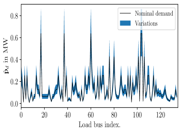
(a)

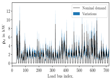
(b)

Figure 2: Nominal load demand and variation in the training set.

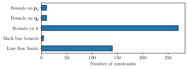
(a)

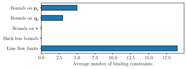
(b)

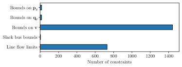
(c)

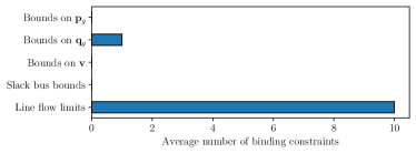
(d)

Figure 3: Total and binding constraints, averaged over the validation set.

TABLE II: Performance evaluation of different constraint classification approaches is based on the solving time of the reduced problems and the fraction of re-solves required for samples in the validation sets. ‘True Positive’ occurs when a binding constraint is correctly classified as binding. ‘True Negative’ occurs when a non-binding constraint is correctly classified as non-binding. ‘False Positive’ occurs when a non-binding constraint is incorrectly classified as binding. ‘False Negative’ occurs when a binding constraint is incorrectly classified as non-binding.

Method of Constr. Removal	Confusion Matrix				Total Solve Time	Fraction Resolved
	True Positive	True Negative	False Positive	False Negative
141-Bus System
Unreduced Problem	1.83%	98.17%	-	-	6.802s	-
ICNN and Dual Vars.	1.64%	93.58%	4.58%	0.19%	2.400s	0.000
Deep Classifier	0.91%	97.70%	0.47%	0.92%	3.034s	0.627
Decision Tree Classifier	1.28%	97.78%	0.38%	0.55%	2.727s	0.431
Ridge Classifier	0.93%	97.79%	0.38%	0.91%	3.170s	0.705
730-Bus System
Unreduced Problem	0.35%	99.65%	-	-	37.033s	-
ICNN and Dual Vars.	0.35%	99.50%	0.15%	0.00%	8.977s	0.000
Deep Classifier	0.18%	99.65%	0.00%	0.17%	17.566s	0.980
Decision Tree Classifier	0.20%	99.61%	0.04%	0.15%	11.826s	0.313
Ridge Classifier	0.22%	99.64%	0.01%	0.14%	16.977s	0.980

In this section, we investigate the training algorithm 1 and the algorithm for accelerated C-OPF (2). For the same we use the socp-dOPF model introduced in (7). The test radial networks use a 141-bus system in MATPOWER [33] and a 730-bus radial system in [34]. Available data for both systems provide network topology, line parameters, and load demands. For the 141-bus system, the line flow limits are taken as 1.5 times the nominal flow limits, while for the 730-bus system, line flow limits are computed from the line ampacity (i.e. maximum value of $\boldsymbol{\ell}$) by assuming unity voltage values (in p.u.) and using (4d). We add distributed generation to both systems, with 5 generator buses in the 141-bus and 25 generator buses in the 730-bus system. The parameters and constraints are summarized in Table I.

To implement Algorithm 1, we use MATLAB and CVX [35], and for training NN, we employ PyTorch. The codes are executed on a PC with an Intel Core i7 processor, 32 GiB of RAM, and an NVidia 1660Ti graphics card. When generating dataset $\mathcal{D}_{1}$, parameters are sampled within a range of 25% around their nominal values. For $\mathcal{D}_{2}$, we generate 600 randomly sampled convex combinations of parameters from $\mathcal{D}_{1}$. The resulting combined dataset $\mathcal{D}=\mathcal{D}_{1}\cup\mathcal{D}_{2}$ is then split into train and validation sets, with the latter containing 50 data points, and the remainder allocated to the former. Figure 2 illustrates variations in real power demand $\hat{\mathbf{p}}_{d}$ for both 141- and 730-bus systems within the training set. Note that real power demand is just one part of the total parameter vector, and each index of the parameter vector is independently sampled. Figure 3 displays the number of constraints in the original C-OPF for both systems, compared to the number of constraints that are actually binding at the optimum. This reveals that a substantial number of constraints are non-binding and consequently only serve to slow down the underlying solver.

Our design of ICNN NN involves 3 convex layers and LeakyReLU activation function with parameter $\alpha=0.1$. Once NN has been trained via Algorithm 1, the parameters that were saved in the validation set are fed in Algorithm 2 to notice the acceleration of C-OPF. Note that the task of recognizing binding constraints given the parameters essentially boils down to learning a mapping of the form $(\boldsymbol{\gamma},\boldsymbol{\xi})\mapsto\{0,1\}^{\tilde{L}}$. Thus, we compare the proposed ICNN-based approach with three other popular classification schemes:

• Scheme 1 involves a DNN with sigmoid outputs [36]. This DNN takes the parameters $(\boldsymbol{\gamma},\boldsymbol{\lambda})$ as input and produces $\tilde{L}$ scalars in the range $(0,1)$ as output, representing the probability of each of the $\tilde{L}$ constraints binding. We employ a 3-layer DNN and train it on dataset $\mathcal{D}_{1}$ using binary cross-entropy loss as the loss function.

• Scheme 2 entails training a decision-tree classifier on dataset $\mathcal{D}_{1}$ to learn the binding constraints as a function of parameters. The decision tree implementation available in the sklearn package is used.

• Scheme 3 trains a ridge regression classifier on $\mathcal{D}_{1}$ using the sklearn package. The ridge regression classifier initially converts the targets (indicating binding and non-binding constraints) to ${-1,1}$ and subsequently fits a linear model, mapping the input parameters to targets using ridge regression.

The comparative results are presented in Table II, including the confusion matrix, total solve times, and the fraction of cases requiring resolution due to the detection of violated constraints. All values in Table II are computed over the validation set containing 50 elements.

Immediately, it is evident that the proposed ICNN-based CS method exhibits high true positives and low false negatives but faces relatively lower true negatives and higher false positives. However, we argue that this behavior is acceptable. In the task of classifying constraints, it is crucial to minimize false negatives (leading to an increase in true positives), with a secondary emphasis on minimizing false positives (leading to an increase in true negatives). This is because misclassifying a binding constraint as non-binding may result in a constraint violation in the reduced problem in Algorithm 2, prompting a re-solve with additional violated constraints. Such a re-solve significantly increases the total runtime of Algorithm 2. It is evident that the very low false negatives achieved by the ICNN-based CS on both test systems helps it avoid re-solves entirely, thereby achieving the lowest solve times. Another noteworthy observation is that the decision tree classifier performs better on both test systems compared to the DNN-based classifier, highlighting that the superiority of ICNN arises from its convexity rather than being solely due to its deep-learning-based architecture. Lastly, it should be noted that all CS methods result in lower solve times compared to the unreduced problem, underscoring the importance of incorporating CS in any convex solver to significantly accelerate it.

V Conclusion

In this paper, we introduce a data-driven constraint screening approach to expedite convexified optimal power flow, utilizing the architecture of input-convex neural networks. We present a general technique based on rank conditions to assess the suitability of a given convexified OPF model for acceleration and explore methods for dataset generation and augmentation across OPF parameters. Numerical simulations illustrate that the proposed method significantly reduces the solving times for large-scale OPF problems while ensuring the same solution as the unreduced problem. Future research directions include incorporating switching topology, such as line connectivity and parameters, into the pre-solver. Additionally, we aim to leverage duality theory techniques employed in this work to accelerate distributed OPF in a data-driven manner.

-A Proof of Theorem 1

The proof of Theorem 1 uses a modified version of results presented in [37]. First, we consider the following parameterized problem (not necessarily convex).

$$\mathcal{P}(\boldsymbol{\theta})\stackrel{{\scriptstyle\Delta}}{{=}}\min\limits_{\mathbf{x}\in n}\quad f(\mathbf{x})$$

s.t. $$g(\mathbf{x})\preceq\mathbf{0},\quad h(\mathbf{x})=\mathbf{0}$$

$$\tilde{g}(\mathbf{x},\boldsymbol{\theta})\preceq\mathbf{0},\quad\tilde{h}(\mathbf{x},\boldsymbol{\theta})=\mathbf{0}$$

We define the fixed and parameterized feasible sets as

$$\mathcal{X}_{f} \stackrel{{\scriptstyle\Delta}}{{=}}\{\mathbf{x}:g(\mathbf{x})\preceq\mathbf{0},h(\mathbf{x})=\mathbf{0}\}$$

$$\mathcal{X}_{\boldsymbol{\theta}} \stackrel{{\scriptstyle\Delta}}{{=}}\{\mathbf{x}:\text{$\mathbf{x}$ is a feasible point for $\mathcal{P}(\boldsymbol{\theta})$}\}.$$

Note that $\mathcal{X}_{f}$ is the analogue of $\mathcal{X}_{\mathrm{pf}}$ used in Theorem 1. The following result combines Assumption 1 and Theorem 2 in [37].

Theorem.

Assume that for all $\mathbf{x}\in\mathcal{X}_{f}$, the Linear Independence Constraint Qualification (LICQ) holds, i.e.,

$$\text{rank}\left\{\begin{bmatrix}\nabla_{\mathbf{x}}[g(\mathbf{x})]_{\mathcal{A}_{g}(\mathbf{x})}\\ \nabla_{\mathbf{x}}h(\mathbf{x})\end{bmatrix}\right\}=\text{dim}(h(\mathbf{x}))+|\mathcal{A}_{g}(\mathbf{x})|,$$

and further assume that $f,g,h,\tilde{g},\tilde{h}$ are infinitely differentiable. Let $\boldsymbol{\theta}\in\Theta$ where $\Theta$ is a set of non-zero measure. If the map

$$\boldsymbol{\theta}\mapsto(\tilde{g}(\mathbf{x},\boldsymbol{\theta}),\tilde{h}(\mathbf{x},\boldsymbol{\theta}))$$

has rank $\text{dim}(\tilde{g}(\mathbf{x},\boldsymbol{\theta}))+\text{dim}(\tilde{h}(\mathbf{x},\boldsymbol{\theta}))$ for every $\mathbf{x}\in\mathcal{X}_{f}$, then LICQ holds jointly for all constraints in $\mathcal{P}(\boldsymbol{\theta})$ almost everywhere in $\Theta$.

We note that the assumptions in Theorem 1 are similar to the above theorem except for the rank condition for the parameter map. However, the condition holds trivially because in C-OPF (1) we have

$$\boldsymbol{\theta}\equiv(\boldsymbol{\gamma},\boldsymbol{\xi}),\quad\tilde{g}(\mathbf{x},\boldsymbol{\theta})\equiv\tilde{g}(\mathbf{x})-\boldsymbol{\gamma},\quad\tilde{h}(\mathbf{x},\boldsymbol{\theta})\equiv\tilde{h}(\mathbf{x})-\boldsymbol{\xi},$$

and correspondingly the mapping

$$\boldsymbol{\theta}\mapsto(\tilde{g}(\mathbf{x},\boldsymbol{\theta}),\tilde{h}(\mathbf{x},\boldsymbol{\theta}))\equiv(\boldsymbol{\gamma},\boldsymbol{\xi})\mapsto(\tilde{g}(\mathbf{x})-\boldsymbol{\gamma},\tilde{h}(\mathbf{x})-\boldsymbol{\xi})$$

is the negative identity, and therefore full-rank. Thus, LICQ is shown to hold for almost all $(\boldsymbol{\gamma},\boldsymbol{\xi})\in\Gamma\times\Xi$. LICQ ensures the existence of unique dual variables which satisfy KKT first order optimality conditions [37, Theorem 1], which for convex problems is a sufficient condition for strong duality, implying $\mathcal{J}(\boldsymbol{\gamma},\boldsymbol{\xi})=-\boldsymbol{\tilde{\lambda}}^{*\top}\boldsymbol{\gamma}-\boldsymbol{\tilde{\mu}}^{*\top}\boldsymbol{\xi}+W$, where $W$ denotes additional terms not involving $\boldsymbol{\gamma}$ or $\boldsymbol{\xi}$ (cf. (9)). The closed forms of $\nabla_{\boldsymbol{\gamma}}\mathcal{J}(\boldsymbol{\gamma},\boldsymbol{\xi})$ and $\nabla_{\boldsymbol{\xi}}\mathcal{J}(\boldsymbol{\gamma},\boldsymbol{\xi})$ follow.

-B Proof of Proposition 2

We begin this proof by writing the relaxed DistFlow equations in a vector-matrix form. To that end, we define the line-bus incidence matrix of $\mathcal{G}$, denoted as $\tilde{\mathbf{A}}\in n_{b}\times(n_{b}+1)$ as

$$\tilde{\mathbf{A}}_{ij}=\begin{cases}1,&\text{if $\exists$ $i\in\mathcal{L}$ s.t. $i\equiv j\rightarrow k$ for $j,k\in\hat{\mathcal{N}}_{0}$}\\ -1,&\text{if $\exists$ $i\in\mathcal{L}$ s.t. $i\equiv k\rightarrow j$ for $j,k\in\hat{\mathcal{N}}_{0}$}\\ 0,&\text{otherwise},\end{cases}$$

where $\hat{\mathcal{N}}_{0}\stackrel{{\scriptstyle\Delta}}{{=}}\{i+1:i\in\mathcal{N}_{0}\}$ is the set $\mathcal{N}_{0}$ but with every index increased by 1. We can represent $\tilde{\mathbf{A}}$ as $\tilde{\mathbf{A}}=[\mathbf{a}_{0},\mathbf{A}]$, where $\mathbf{A}\in n_{b}\times n_{b}$ is the reduced line-bus incidence matrix. Further, let $\mathbf{F}\stackrel{{\scriptstyle\Delta}}{{=}}\mathbf{A}^{-1}$. It is known that $\mathbf{F}$ exists since $\mathcal{G}$ is a tree. We define the resistance and reactance diagonal matrices as $\mathbf{D}_{r}\stackrel{{\scriptstyle\Delta}}{{=}}\text{diag}(\{r_{l}\}_{l\in\mathcal{L}})$ and $\mathbf{D}_{x}\stackrel{{\scriptstyle\Delta}}{{=}}\text{diag}(\{x_{l}\}_{l\in\mathcal{L}})$. We define the matrices $\mathbf{R}$ and $\mathbf{X}$ as

$$\mathbf{R}\stackrel{{\scriptstyle\Delta}}{{=}}2\mathbf{F}\mathbf{D}_{r}\mathbf{F}^{\top},\quad\mathbf{X}\stackrel{{\scriptstyle\Delta}}{{=}}2\mathbf{F}\mathbf{D}_{x}\mathbf{F}^{\top}.$$

Lastly, we define the ‘parent’ voltage vector as $\mathbf{v}_{\pi}=[\mathbf{v}_{\pi_{1}},\mathbf{v}_{\pi_{2}},\dots,\mathbf{v}_{\pi_{n_{b}}}]^{\top}$. The vector-matrix form of DistFlow equations are given as [38]:

$$\mathbf{p}-\mathbf{A}^{\top}\mathbf{P}-\mathbf{D}_{r}\boldsymbol{\ell}=\mathbf{0}$$ (11a)

$$\mathbf{q}-\mathbf{A}^{\top}\mathbf{Q}-\mathbf{D}_{x}\boldsymbol{\ell}=\mathbf{0}$$ (11b)

$$\mathbf{Av}+\mathbf{a}_{0}\hat{v}_{0}-2\mathbf{D}_{r}\mathbf{P}-2\mathbf{D}_{x}\mathbf{Q}+(\mathbf{D}_{r}^{2}+\mathbf{D}_{x}^{2})\boldsymbol{\ell}=\mathbf{0}$$ (11c)

$$\text{diag}(\mathbf{P})\mathbf{P}+\text{diag}(\mathbf{Q})\mathbf{Q}-\text{diag}(\boldsymbol{\ell})\mathbf{v}_{\pi}\preceq\mathbf{0}.$$ (11d)

We denote by $\mathcal{A}_{\mathbf{x}}\subseteq[n_{b}]$ the set of inequalities (11d) which are binding for the given $\mathbf{x}$. Let $[\mathbf{M}]_{\mathcal{A}}$ denote the rows of matrix $\mathbf{M}$ indexed by $\mathcal{A}$. $\mathbf{I}_{n}$ denotes the identity matrix of size $n$ and $\mathbf{0}_{mn}$ denotes the zero matrix of size $m\times n$. The gradient of the above equations with respect to the optimization variables $\mathbf{x}=(\mathbf{p},\mathbf{q},\mathbf{v},\mathbf{P},\mathbf{Q},\boldsymbol{\ell})$ is given by $[\mathbf{R}_{1},\mathbf{R}_{2}]$, where

$$\mathbf{R}_{1} \stackrel{{\scriptstyle\Delta}}{{=}}\begin{bmatrix}\mathbf{I}_{n_{b}}&\mathbf{0}_{n_{b}n_{b}}&\mathbf{0}_{n_{b}n_{b}}\\ \mathbf{0}_{n_{b}n_{b}}&\mathbf{I}_{n_{b}}&\mathbf{0}_{n_{b}n_{b}}\\ \mathbf{0}_{n_{b}n_{b}}&\mathbf{0}_{n_{b}n_{b}}&\mathbf{A}\\ \mathbf{0}_{|\mathcal{A}_{\mathbf{x}}|n}&\mathbf{0}_{|\mathcal{A}_{\mathbf{x}}|n}&\left[\text{diag}(\boldsymbol{\ell})\frac{\partial\mathbf{v}_{\pi}}{\partial\mathbf{v}}\right]_{\mathcal{A}_{\mathbf{x}}}\end{bmatrix}$$

$$\mathbf{R}_{2} \stackrel{{\scriptstyle\Delta}}{{=}}\begin{bmatrix}-\mathbf{A}^{\top}&\mathbf{0}_{n_{b}n_{b}}&-\mathbf{D}_{r}\\ \mathbf{0}_{n_{b}n_{b}}&-\mathbf{A}^{\top}&-\mathbf{D}_{x}\\ -2\mathbf{D}_{r}&-2\mathbf{D}_{x}&\mathbf{D}_{r}^{2}+\mathbf{D}_{x}^{2}\\ 2[\text{diag}(\mathbf{P})]_{\mathcal{A}_{\mathbf{x}}}&2[\text{diag}(\mathbf{Q})]_{\mathcal{A}_{\mathbf{x}}}&[\text{diag}(\mathbf{v}_{\pi})]_{\mathcal{A}_{\mathbf{x}}}\end{bmatrix}.$$

Note that the derivative matrix $[\mathbf{R}_{1},\mathbf{R}_{2}]\in\mathbb{R}^{\left(3n_{b}+|\mathcal{A}_{\mathbf{x}}|\right)\times 6n_{b}}$ can have a maximum row rank of $3n_{b}+|\mathcal{A}_{\mathbf{x}}|$. Using the following helper result, we show that $[\mathbf{R}_{1},\mathbf{R}_{2}]\in\mathbb{R}^{\left(3n_{b}+|\mathcal{A}_{\mathbf{x}}|\right)\times 6n_{b}}$ does achieve said rank.

Claim.

For a given value of $\mathbf{x}$, consider the matrix $\mathbf{\tilde{R}}\in\left(n_{b}+|\mathcal{A}_{\mathbf{x}}|\right)\times 2n_{b}$ given as

$$\tilde{\mathbf{R}}\stackrel{{\scriptstyle\Delta}}{{=}}\begin{bmatrix}\mathbf{A}&\mathbf{D}_{r}^{2}+\mathbf{D}_{x}^{2}\\ \left[\text{diag}(\boldsymbol{\ell})\frac{\partial\mathbf{v}_{\pi}}{\partial\mathbf{v}}\right]_{\mathcal{A}_{\mathbf{x}}}&\left[\text{diag}(\mathbf{v}_{\pi})\right]_{\mathcal{A}_{\mathbf{x}}}\end{bmatrix}.$$

$\tilde{\mathbf{R}}$ has full (row) rank.

Proof.

Using the fact that $\mathbf{v}_{\pi}=(\mathbf{A}+\mathbf{I}_{n_{b}})\mathbf{v}+\mathbf{a}_{0}\hat{v}_{0}$, we have

$$\tilde{\mathbf{R}}\stackrel{{\scriptstyle\Delta}}{{=}}\begin{bmatrix}\mathbf{A}&\mathbf{D}_{r}^{2}+\mathbf{D}_{x}^{2}\\ \left[\text{diag}(\boldsymbol{\ell})\right]_{\mathcal{A}_{\mathbf{x}}}(\mathbf{A}+\mathbf{I}_{n_{b}})&\left[\text{diag}(\mathbf{v}_{\pi})\right]_{\mathcal{A}_{\mathbf{x}}}\end{bmatrix}.$$

It is evident that the first block-row of $\tilde{\mathbf{R}}$ has linearly independent rows due to invertibility of $\mathbf{A}$, and so does the second block-row due to $\left[\text{diag}(\mathbf{v}_{\pi})\right]_{\mathcal{A}_{\mathbf{x}}}$ being full row-rank (which follows from non-negativity of voltages). We now show that any row in the second block-row is linearly independent from the rows in the first block-row (and vice-versa).

Since both $\mathbf{D}_{r}^{2}+\mathbf{D}_{x}^{2}$ and $\left[\text{diag}(\mathbf{v}_{\pi})\right]_{\mathcal{A}_{\mathbf{x}}}$ are non-negative diagonal matrices, any linear dependence between the former and latter can only involve single rows, and a positive scaling factor. However, the corresponding rows of $\mathbf{A}$ and $\left[\text{diag}(\boldsymbol{\ell})\right]_{\mathcal{A}_{\mathbf{x}}}(\mathbf{A}+\mathbf{I}_{n_{b}})$ cannot be made equal with the same scaling factor, since our choice of line labeling results in $\mathbf{A}$ and $\mathbf{A}+\mathbf{I}_{n_{b}}$ having $-1$’s and $0$’s everywhere on the main diagonal respectively. It follows that all rows of $\tilde{\mathbf{R}}$ are linearly independent, and therefore $\tilde{\mathbf{R}}$ has full row-rank. ∎

Now consider the column submatrix $\mathbf{G}\in\left(3n_{b}+|\mathcal{A}_{\mathbf{x}}|\right)\times 4n_{b}$ of $[\mathbf{R}_{1},\mathbf{R}_{2}]$ given by

$$\mathbf{G}\stackrel{{\scriptstyle\Delta}}{{=}}\begin{bmatrix}\mathbf{I}_{n_{b}}&\mathbf{0}_{n_{b}n_{b}}&[\mathbf{0}_{n_{b}n_{b}},-\mathbf{D}_{r}]\\ \mathbf{0}_{n_{b}n_{b}}&\mathbf{I}_{n_{b}}&[\mathbf{0}_{n_{b}n_{b}},-\mathbf{D}_{x}]\\ \mathbf{0}_{\left(n_{b}+|\mathcal{A}_{\mathbf{x}}|\right)n_{b}}&\mathbf{0}_{\left(n_{b}+|\mathcal{A}_{\mathbf{x}}|\right)n_{b}}&\tilde{\mathbf{R}}.\end{bmatrix}$$

Since $\mathbf{G}$ is a block upper-triangular matrix, it follows from [39, Section 0.9.4] and the above claim that

$$\text{rank}(\mathbf{G}) \geq\text{rank}(\mathbf{I}_{n_{b}})+\text{rank}(\mathbf{I}_{n_{b}})+\text{rank}(\tilde{\mathbf{R}})$$

$$=3n_{b}+|\mathcal{A}_{\mathbf{x}}|.$$

Since $\mathbf{G}$ is constituted of a subset of columns of $[\mathbf{R}_{1},\mathbf{R}_{2}]$, it follows that the latter is full rank.

-C Proof of Lemma 2

For brevity, we consider the simpler problem,

$$\min\limits_{\mathbf{x}\in n}\quad f(\mathbf{x})\quad\text{s.t.}\quad\tilde{g}(\mathbf{x})\preceq\boldsymbol{\gamma},$$

with $\tilde{g}:n\mapsto\tilde{L}$, because the justification carries over to the full C-OPF (1). If the above problem satisfies LICQ as laid out in Theorem 1, the KKT conditions, which are necessary for global optimality of convex problems, are given as

$$\nabla_{\mathbf{x}^{*}}\left(f(\mathbf{x})+\tilde{\boldsymbol{\lambda}}^{*\top}(\tilde{g}(\mathbf{x}^{*})-\boldsymbol{\gamma})\right)\in\mathbf{0}$$

$$\tilde{g}(\mathbf{x}^{*})\preceq\boldsymbol{\gamma},\quad\tilde{\boldsymbol{\lambda}}^{*}\succeq\mathbf{0},\quad\tilde{\boldsymbol{\lambda}}^{*\top}(\tilde{g}(\mathbf{x}^{*})-\boldsymbol{\gamma})=0$$

If it is known a priori that $[\tilde{\boldsymbol{\lambda}}^{*}]_{\mathcal{I}}=\mathbf{0}$, then with the aid of Assumption 1, the KKT conditions can be re-written as

$$\nabla_{\mathbf{x}^{*}}\left(f(\mathbf{x})+[\tilde{\boldsymbol{\lambda}}^{*}]^{\top}_{[\tilde{L}]\setminus\mathcal{I}}[\tilde{g}(\mathbf{x}^{*})-\boldsymbol{\gamma}]_{[\tilde{L}]\setminus\mathcal{I}}\right)\in\mathbf{0}$$

$$[\tilde{g}(\mathbf{x}^{*})]_{[\tilde{L}]\setminus\mathcal{I}}\preceq[\boldsymbol{\gamma}]_{[\tilde{L}]\setminus\mathcal{I}},\quad[\tilde{\boldsymbol{\lambda}}^{*}]^{\top}_{[\tilde{L}]\setminus\mathcal{I}}\succeq\mathbf{0},$$

$$[\tilde{\boldsymbol{\lambda}}^{*}]^{\top}_{[\tilde{L}]\setminus\mathcal{I}}[\tilde{g}(\mathbf{x}^{*})-\boldsymbol{\gamma}]_{[\tilde{L}]\setminus\mathcal{I}}=0,$$

which are exactly the KKT conditions for the reduced problem. Therefore, the optimal points of both problems coincide.

-D Proof of Proposition 4

Let $\{\alpha_{k}\}_{k\in[K]}$ be in a standard simplex (i.e., $\alpha_{k}\geq 0$ and $\sum_{k\in[K]}\alpha_{k}=1$) and $\mathbf{x}^{(k)}$ be feasible to (1) with parameters $(\boldsymbol{\gamma}_{k},\boldsymbol{\xi}_{k})$. Consider a point $\hat{\mathbf{x}}\stackrel{{\scriptstyle\Delta}}{{=}}\sum_{k\in[K]}\alpha_{k}\mathbf{x}^{(k)}$, and note that

$$\tilde{g}(\hat{\mathbf{x}})\stackrel{{\scriptstyle[a]}}{{\preceq}}\sum_{k\in[K]}\alpha_{k}\tilde{g}(\mathbf{x}^{(k)})\preceq\sum_{k\in[K]}\alpha_{k}\boldsymbol{\gamma}_{k},$$

wherein $[a]$ follows from the elementwise convexity of $\tilde{g}(\mathbf{x})$. Similarly, it can be shown that $\hat{\mathbf{x}}$ satisfies the remaining constraints of (1) with the parameters $\left(\sum_{k\in[K]}\alpha_{k}\boldsymbol{\gamma}_{k},\sum_{k\in[K]}\alpha_{k}\boldsymbol{\xi}_{k}\right)$. This established the claim that the problem defined by any convex combination of feasible input parameters has a feasible point.

-E Proof of Proposition 3

We again consider the simplified version of C-OPF

$$\mathcal{J}(\boldsymbol{\gamma})\stackrel{{\scriptstyle\Delta}}{{=}}\min\limits_{\mathbf{x}\in n}\quad f(\mathbf{x})\quad\text{s.t.}\quad\tilde{g}(\mathbf{x})\preceq\boldsymbol{\gamma},$$

with $\tilde{g}:n\mapsto\tilde{L}$, and the proof presented generalizes to (1). Furthermore, Theorem 1 and the assumption of this proposition imply that $\nabla_{\boldsymbol{\gamma}}\mathcal{J}(\boldsymbol{\gamma})$ is unique, and therefore $\mathcal{J}(\boldsymbol{\gamma})$ is differentiable at $\boldsymbol{\gamma}$.

Let $\nabla_{\boldsymbol{\gamma}}\mathcal{J}(\boldsymbol{\gamma})=-\tilde{\boldsymbol{\lambda}}^{*}$, with misclassification on indices $\mathcal{B}\subseteq[\tilde{L}]$, i.e. $[\tilde{\boldsymbol{\lambda}}^{*}]_{\mathcal{B}}\succ\mathbf{0}$. Consider the vector $\Delta\boldsymbol{\gamma}$ given as

$$\Delta\boldsymbol{\gamma}_{i}=\begin{cases}0&\text{if }i\not\in\mathcal{B}\\ 1&\text{if }i\in\mathcal{B}.\end{cases}$$

The differentiability of $\mathcal{J}(\boldsymbol{\gamma})$ at $\boldsymbol{\gamma}$ implies that $\mathcal{J}$ is strictly decreasing in all directions where $\Delta\boldsymbol{\gamma}$ is nonzero. Equivalently, there exists $\epsilon>0$ such that $\mathcal{J}(\boldsymbol{\gamma}+\epsilon\Delta\boldsymbol{\gamma})<\mathcal{J}(\boldsymbol{\gamma})$. This implies that a positive perturbation to $\boldsymbol{\gamma}$ in the direction of (any subset of) $\mathcal{B}$ will result in a lower cost for C-OPF $\mathcal{J}$ while the constraints themselves are violated. Furthermore it follows from $\nabla_{\boldsymbol{\gamma}}\mathcal{J}(\boldsymbol{\gamma})\preceq\mathbf{0}$ that $\mathcal{J}(\boldsymbol{\gamma}+\epsilon_{1}\Delta\boldsymbol{\gamma})\succeq\mathcal{J}(\boldsymbol{\gamma}+\epsilon_{2}\Delta\boldsymbol{\gamma})$ for non-negative $\epsilon_{1}<\epsilon_{2}$.

Combining the two aforementioned observations, we see that the C-OPF defined as $\lim\limits_{\epsilon\rightarrow+\infty}\mathcal{J}(\boldsymbol{\gamma}+\epsilon\Delta\boldsymbol{\gamma})$ is strictly smaller than $\mathcal{J}(\boldsymbol{\gamma})$ and violates the constraints in $\mathcal{B}$. We conclude the proof by observing that $\lim\limits_{\epsilon\rightarrow+\infty}\mathcal{J}(\boldsymbol{\gamma}+\epsilon\Delta\boldsymbol{\gamma})$ is equivalent to eliminating the binding constraints $\mathcal{B}$ from $\mathcal{J}(\boldsymbol{\gamma})$.

References

- [1] W. A. Bukhsh, A. Grothey, K. I. M. McKinnon, and P. A. Trodden, “Local solutions of the optimal power flow problem,” IEEE Trans. Power Syst., vol. 28, no. 4, pp. 4780–4788, 2013.
- [2] A. J. Wood, B. F. Wollenberg, and G. B. Sheblé, Power generation, operation, and control. John Wiley & Sons, 2013.
- [3] M. E. Baran and F. F. Wu, “Optimal capacitor placement on radial distribution systems,” IEEE Transactions on Power Delivery, vol. 4, no. 1, pp. 725–734, 1989.
- [4] R. A. Jabr, “Radial distribution load flow using conic programming,” IEEE Trans. Power Syst., vol. 21, no. 3, pp. 1458–1459, 2006.
- [5] M. Farivar, C. R. Clarke, S. H. Low, and K. M. Chandy, “Inverter VAR control for distribution systems with renewables,” in 2011 IEEE Intl Conf. on Smart Grid Commun., pp. 457–462.
- [6] M. Farivar and S. H. Low, “Branch flow model: Relaxations and convexification—part I,” IEEE Trans. Power Syst., vol. 28, no. 3, pp. 2554–2564, 2013.
- [7] N. Li, L. Chen, and S. H. Low, “Exact convex relaxation of opf for radial networks using branch flow model,” in 2012 IEEE Third Intl Conf. on Smart Grid Commun., pp. 7–12.
- [8] X. Bai, H. Wei, K. Fujisawa, and Y. Wang, “Semidefinite programming for optimal power flow problems,” International Journal of Electrical Power & Energy Systems, vol. 30, no. 6-7, pp. 383–392, 2008.
- [9] R. Madani, S. Sojoudi, and J. Lavaei, “Convex relaxation for optimal power flow problem: Mesh networks,” IEEE Trans. Power Syst., vol. 30, no. 1, pp. 199–211, 2015.
- [10] J. Lavaei and S. H. Low, “Zero duality gap in optimal power flow problem,” IEEE Trans. Power Syst., vol. 27, no. 1, pp. 92–107, 2012.
- [11] C. Coffrin, H. L. Hijazi, and P. Van Hentenryck, “The QC relaxation: A theoretical and computational study on optimal power flow,” IEEE Trans. Power Syst., vol. 31, no. 4, pp. 3008–3018, 2016.
- [12] B. Kocuk, S. S. Dey, and X. A. Sun, “Strong SOCP relaxations for the optimal power flow problem,” Operations Research, vol. 64, no. 6, pp. 1177–1196, 2016.
- [13] S. Bose, S. H. Low, T. Teeraratkul, and B. Hassibi, “Equivalent relaxations of optimal power flow,” IEEE Transactions on Automatic Control, vol. 60, no. 3, pp. 729–742, 2015.
- [14] D. K. Molzahn and I. A. Hiskens, “A survey of relaxations and approximations of the power flow equations,” Foundations and Trends® in Electric Energy Systems, vol. 4, no. 1-2, pp. 1–221, 2019.
- [15] J. Telgen, “Identifying redundant constraints and implicit equalities in systems of linear constraints,” Management Science, vol. 29, no. 10, pp. 1209–1222, 1983.
- [16] G. L. Thompson, F. M. Tonge, and S. Zionts, “Techniques for removing nonbinding constraints and extraneous variables from linear programming problems,” Management Science, vol. 12, no. 7, pp. 588–608, 1966.
- [17] Z. J. Zhang, P. T. Mana, D. Yan, Y. Sun, and D. K. Molzahn, “Study of active line flow constraints in DC optimal power flow problems,” in 2020 SoutheastCon, 2020, pp. 1–8.
- [18] B. Hua, Z. Bie, C. Liu, G. Li, and X. Wang, “Eliminating redundant line flow constraints in composite system reliability evaluation,” IEEE Trans. Power Syst., vol. 28, no. 3, pp. 3490–3498, 2013.
- [19] R. Weinhold and R. Mieth, “Fast security-constrained optimal power flow through low-impact and redundancy screening,” IEEE Trans. Power Syst., vol. 35, no. 6, pp. 4574–4584, 2020.
- [20] R. Madani, J. Lavaei, and R. Baldick, “Constraint screening for security analysis of power networks,” IEEE Trans. Power Syst., vol. 32, no. 3, pp. 1828–1838, 2017.
- [21] S. Pineda, J. M. Morales, and A. Jiménez-Cordero, “Data-driven screening of network constraints for unit commitment,” IEEE Trans. Power Syst., vol. 35, no. 5, pp. 3695–3705, 2020.
- [22] S. Zhang, H. Ye, F. Wang, Y. Chen, S. Rose, and Y. Ma, “Data-aided offline and online screening for security constraint,” IEEE Trans. Power Syst., vol. 36, no. 3, pp. 2614–2622, 2021.
- [23] A. Porras, S. Pineda, J. M. Morales, and A. Jiménez-Cordero, “Cost-driven screening of network constraints for the unit commitment problem,” IEEE Trans. Power Syst., vol. 38, no. 1, pp. 42–51, 2023.
- [24] D. Deka and S. Misra, “Learning for DC-OPF: Classifying active sets using neural nets,” in 2019 IEEE Milan PowerTech, 2019, pp. 1–6.
- [25] F. Hasan and A. Kargarian, “Topology-aware learning assisted branch and ramp constraints screening for dynamic economic dispatch,” IEEE Trans. Power Syst., vol. 37, no. 5, pp. 3495–3505, 2022.
- [26] F. Fioretto, T. W. Mak, and P. Van Hentenryck, “Predicting AC optimal power flows: Combining deep learning and lagrangian dual methods,” Proceedings of the AAAI Conference on Artificial Intelligence, vol. 34, no. 01, pp. 630–637, Apr. 2020.
- [27] M. K. Singh, V. Kekatos, and G. B. Giannakis, “Learning to solve the ac-opf using sensitivity-informed deep neural networks,” IEEE Trans. Power Syst., vol. 37, no. 4, pp. 2833–2846, 2022.
- [28] R. Nellikkath and S. Chatzivasileiadis, “Physics-informed neural networks for AC optimal power flow,” Electric Power Systems Research, vol. 212, p. 108412, 2022.
- [29] L. Zhang, Y. Chen, and B. Zhang, “A convex neural network solver for DCOPF with generalization guarantees,” IEEE Transactions on Control of Network Systems, vol. 9, no. 2, pp. 719–730, 2022.
- [30] D. Bertsimas and J. N. Tsitsiklis, Introduction to linear optimization. Athena scientific Belmont, MA, 1997, vol. 6.
- [31] B. Amos, L. Xu, and J. Z. Kolter, “Input convex neural networks,” in Proceedings of the 34th Intl. Conf. on Machine Learning, ser. Proceedings of Machine Learning Research, D. Precup and Y. W. Teh, Eds., vol. 70. PMLR, 06–11 Aug 2017, pp. 146–155.
- [32] A. Paszke, S. Gross, S. Chintala, G. Chanan, E. Yang, Z. DeVito, Z. Lin, A. Desmaison, L. Antiga, and A. Lerer, “Automatic differentiation in pytorch,” 2017.
- [33] R. D. Zimmerman, C. E. Murillo-Sánchez, and R. J. Thomas, “Matpower: Steady-state operations, planning, and analysis tools for power systems research and education,” IEEE Trans. Power Syst., vol. 26, no. 1, pp. 12–19, 2011.
- [34] H. K. Vemprala, M. A. I. Khan, and S. Paudyal, “Open-source poly-phase distribution system power flow analysis tool (dxflow),” in 2019 IEEE International Conference on Electro Information Technology (EIT), 2019, pp. 1–6.
- [35] M. Grant and S. Boyd, “CVX: Matlab software for disciplined convex programming, version 2.1,” http://cvxr.com/cvx, Mar. 2014.
- [36] D. Deka and S. Misra, “Learning for DC-OPF: Classifying active sets using neural nets,” in 2019 IEEE Milan PowerTech, pp. 1–6.
- [37] A. Hauswirth, S. Bolognani, G. Hug, and F. Dörfler, “Generic existence of unique lagrange multipliers in ac optimal power flow,” IEEE Control Systems Letters, vol. 2, no. 4, pp. 791–796, 2018.
- [38] V. Kekatos, L. Zhang, G. B. Giannakis, and R. Baldick, “Voltage regulation algorithms for multiphase power distribution grids,” IEEE Trans. Power Syst., vol. 31, no. 5, pp. 3913–3923, 2016.
- [39] R. A. Horn and C. R. Johnson, Matrix analysis. Cambridge university press, 2012.