Benchmarking Pretrained Vision Embeddings for Near- and Duplicate Detection in Medical Images

Abstract

Near- and duplicate image detection is a critical concern in the field of medical imaging. Medical datasets often contain similar or duplicate images from various sources, which can lead to significant performance issues and evaluation biases, especially in machine learning tasks due to data leakage between training and testing subsets. In this paper, we present an approach for identifying near- and duplicate 3D medical images leveraging publicly available 2D computer vision embeddings. We assessed our approach by comparing embeddings extracted from two state-of-the-art self-supervised pretrained models and two different vector index structures for similarity retrieval. We generate an experimental benchmark based on the publicly available Medical Segmentation Decathlon dataset. The proposed method yields promising results for near- and duplicate image detection achieving a mean sensitivity and specificity of 0.9645 and 0.8559, respectively.

I Introduction

Near- and duplicate image detection aims to find similar or identical images in a large data corpus and has many applications in web image retrieval and forensic tasks. Most image (near-) duplicate detection algorithms rely on matching images based on distance measures of associated image embeddings. In order to classify (near-) duplicates and non-duplicates typically a distance threshold is used. The most common handcrafted embeddings are SIFT [1] and SURF [2] features. Recent works leverage Deep Learning features [3, 4, 5] or combine with handcrafted features such as SIFT [6] to construct features at local and global level.

In medical imaging, identical or slightly preprocessed images can be sold by different data brokers or even by the same vendor for different tasks. This is in particular risky when machine learning approaches are used. The model performance may be negatively impacted by (near-) duplicates or even evaluation biases might occur due to data leakage between train and test sets as observed in [7]. Developing (near-) duplicate detection algorithms for medical images comes with several challenges. First, most medical images are acquired in 3D and need to be projected to a low-dimensional representation for similarity search. While there are plenty of powerful pre-trained 2D image feature extractors available [8, 9], there is much less work related to 3D feature extraction. Applying 2D embeddings in a slice-wise fashion is not straightforward as well. For example, border slices often contain uninformative background voxels which may cause mismatches with border slices from other cases regardless of anatomy or modality. This has direct implications for robustly calibrating the similarity threshold for duplicate identification. In our approach, we aim to leverage 2D feature extractors pretrained on natural images and propose a count-based matching scheme for 3D image volumes that supports finding an optimal threshold for detecting (near-) duplicates and non-duplicates. Our main contributions are as follows:

• We introduce a matching approach for 3D image volumes that relies on the majority counts from slice-wise retrievals, enabling the identification of a threshold for both near-duplicate and duplicate image detection.

• We synthesize near-duplicates using various image transformations with different distortion levels. The robustness of different pretrained feature embeddings towards these transformations is quantitatively benchmarked.

• We evaluate the detection performance using embeddings extracted by DINO [10, 11], the state-of-the-art self-supervised models designed for natural images, demonstrating the transferability of such models to medical imaging tasks without the need for fine-tuning as studied in [12].

II Methods

We present in this section our proposal for retrieving 3D medical images based on a slice-wise similarity search. As shown in Figure 1, our approach consists of a 2D feature extractor $\phi$ that embeds the 2D slices into a vector representation. Let $X^{(i)}$ be the image volume related to case $i$ in the database and $x^{(i)}_{j}:=\phi(X^{(i)}_{j})$ be the embedding of the $j$-th slice. In our implementation, all embeddings are stored in a vector database that speeds up similarity search. Let $Q$ represent a query image volume consisting of $n$ slices, and $q_{m}:=\phi(Q_{m})$ be the embedding of the $m$-th slice. For all slices $m=1,...,n$ we retrieve the embedding from the database which has minimal cosine-similarity with $q_{m}$ and denote the corresponding volume with $N[q_{m}]$. A histogram is built for all $n$ query slices to identify the case ID in the database with the most hits:

$$h[i]=\sum_{m=1}^{n}\mathds{I}(N[q_{m}],X^{(i)})$$ (1)

Here, $\mathds{I}$ is the identity function that returns 1 if $N[q_{m}]$ matches $X^{(i)}$ and 0 otherwise. The normalized count for top-$k$ predictions is then defined as

$$c(k)=\frac{\sum_{l=1}^{k}h[i_{l}]}{n}$$ (2)

where $i_{1},...,i_{k}$ denote the indices of the $k$ largest hits, i.e. $h[i_{1}]\geq...\geq h[i_{k}]\geq h[j]$ for all $j\not\in\{i_{1},...,i_{k}\}$. The normalized count has a range between 0 and 1. Based on $c(k)$ and a threshold, (near-) duplicates and non-duplicates will be identified. We conduct experiments to finetune this threshold for optimal detection performance and propose in Algorithm 1 a method to find an optimal threshold across different query sets $\mathcal{Q}:=\left\{s_{1},s_{2},...,s_{N}\right\}$. The query sets are different near- and duplicate sets of various image transformations, which are defined in Section IV-A3. We selected a candidate list $\mathbf{T}$ of thresholds based on the Receiver Operating Characteristic (ROC) curve of each query set $s\in\mathcal{Q}$ and chose the final optimal threshold that maximizes the sum of average sensitivity and specificity across all query sets.

Algorithm 1 Finding optimal decision threshold

1:$\mathcal{Q}:=\left\{s_{1},s_{2},...,s_{N}\right\}$

2:init array $\mathbf{T}$, $\mathbf{SE}$, $\mathbf{SP}$

3:for $u=1,2,...,N$ do

4:     $R_{u}:=$ ROC curve for $s_{u}$

5:     $\mathbf{T}[u]\leftarrow t_{ROC}:=\underset{r\in R_{u}}{\textrm{argmax}}(\textrm{sens}[r]+\textrm{spec}[r])$

6:     for $v=1,2,...,N$ do

7:         $\mathbf{SE}[u,v]\leftarrow$ sensitivity of $s_{v}$ at threshold $\mathbf{T}[u]$

8:         $\mathbf{SP}[u,v]\leftarrow$ specificity of $s_{v}$ at threshold $\mathbf{T}[u]$

9:     end for

10:end for

11:$t_{\textrm{opt}}=\mathbf{T}\left[\underset{u=1,...,N}{\textrm{argmax}}\frac{1}{N}\sum_{v=1}^{N}\left(\mathbf{SE}[u,v]+\mathbf{SP}[u,v]\right)\right]$

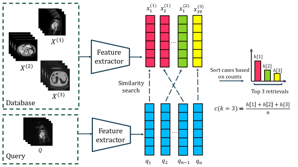
Figure 1: Retrieval at case level based on count accumulation

III Experiments

III-A Datasets

The Medical Segmentation Decathlon (MSD) [13] is a biomedical image analysis challenge comprising segmentation tasks related to different body organs and imaging modalities. The images are either CT or MRI of different sequences that were acquired across multiple institutions and represent real-world data. The dataset was originally split by the challenge organizer into a train and test set which consist of 1723 and 887 cases respectively. To build our benchmark, we further split the MSD train set into 3 buckets 1A, 1B, 1C, and the MSD test set into 3 buckets 2A, 2B, 2C as indicated in Table I. Buckets 1A/2A consist of the first 50% of train/test cases across all tasks and are used to build the database and query for duplicate images. Buckets 1B/2B contain the same cases as buckets 1A/2A but with different image transformations to generate near-duplicate images. Buckets 1C/2C consist of the second 50% of train/test cases and serve as the query for non-duplicate images. We considered each case as a unique patient and leveraged embeddings of different feature extractors, see Section III-B, to retrieve similar images of the query patient in the database. We used buckets 1A/1B/1C to find the decision threshold for (near-) duplicate and non-duplicate classification (see Algorithm 1) and evaluated this threshold on bucket 2A/2B/2C (Table V). Buckets 1B and 2B contain synthetic near-duplicate images by applying the following transformations with package Scipy [14] on original images with different strengths:

• Cropping: crop border in x, y, z dimensions with 5%, 10%, 15%, and 20% of the original full size

• Rotation: rotate the (x, y) plane by 5, 10, 15, and 20 degrees

• Translation: shift the images in x and y dimensions by 5%, 10%, 15%, 20% of the original size

• Blurring: blur images with increasing sigma of 1, 2, 4, and 8

• JPEG Compression: compress images under different quality of 100%, 75%, 50%, and 25%

• Gaussian noise: add Gaussian noise with increasing standard deviation of 0.1, 0.2, 0.4 and 0.8

The first level of strength across all transformations aims to simulate realistic preprocessing steps applied to datasets while the rest 3 levels serve as extreme cases to test the robustness of feature embeddings. Figure 2 shows examples of transformed images of heart MRI images under 4 different strength levels of all 6 proposed transformations.

TABLE I: The number of cases per bucket

	Bucket 1	Bucket 2	Usage
A	859	443	Database & duplicate query
B	859	443	Synthetic near-duplicate query
C	864	444	Non-duplicate query

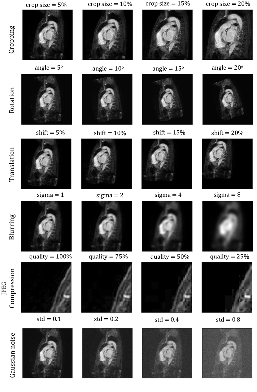
Figure 2: Near-duplicate images generated by geometric and intensity transformations under different strengths. For JPEG compression, a region of interest is shown to display the quality degradation which is not visible under human eyes when looking at the whole image.

III-B Feature extraction and indexing

Our selected feature extractors are DINOv1 [10] and DINOv2 [11], which are powerful self-supervised pretrained models on natural images. The image preprocessing steps included min-max scaling of images to 0-1 and resizing the axial slices to 224$\times$224. Embeddings in buckets 1A and 2A are indexed with Locality-Sensitivity Hashing (LSH) [15] and Hierarchical Navigable Small World (HNSW) [16] for effective similarity search.

III-C Evaluation

We evaluated the classification in two stages. In the first stage, a query image is considered duplicate if $c(k)$ surpasses a threshold value $t$ and non-duplicate otherwise. Here we considered $c(1)$ and $c(3)$ for top-1 and top-3 retrievals, respectively. We used the Area Under the Curve of the Receiver Operating Characteristic (AUC-ROC) to evaluate the class separability at different threshold values. In the second stage, we took the threshold $t_{ROC}$, defined in line 5 of Algorithm 1, to classify the queries into positive and negative outputs. Subsequently, we compared the highest-count case ID $X^{(i_{1})}$ from each case classified as duplicate to the ground-truth case IDs. If a match is found, the query output is classified as a true positive. Otherwise, it is labeled as a false positive. We computed in this stage the sensitivity and specificity values associated with $t_{ROC}$.

IV Results

IV-A Decision threshold determination

In this section, we analyzed embeddings from buckets 1A, 1B, and 1C to determine the best threshold for (near-) duplicate detection using Algorithm 1.

IV-A1 Duplicate vs. Non-duplicate

As an overview of all thresholds, Table II displays the AUC for the first stage evaluation. The top-1 retrieval achieves AUC in the range of 0.98-0.99, while the top-3 retrievals exhibit a slight decrease to 0.96-0.98. Figure 3 illustrates the accumulated count distribution for top-1 and top-3 retrievals indexed by HNSW using DINOv1 embeddings. It is evident that extending from top-1 to top-3 retrievals results in a significant increase in counts, boosting sensitivity while decreasing specificity due to higher false positives. We identified $t_{ROC}$ for all top-k retrievals and computed the associated sensitivity and specificity for the second stage (Table II). Stage 2 maintains a stable sensitivity rate of 0.99 across top-k retrievals, with slightly lower specificity in the top 3 due to increased false positives in the first stage. However, false positives stemming from case ID mismatches in the second stage are relatively low. We also observed that HNSW indexing offers slightly higher sensitivity than LSH, while LSH provides higher specificity compared to HNSW. In terms of extractors, DINOv2 outperformed DINOv1 by a small margin.

TABLE II: (Bucket 1A-1C) Duplicate detection evaluation

		DINOv1		DINOv2
		LSH	HNSW	LSH	HNSW
AUC	Top 1	0.9884	0.9873	0.9901	0.9898
(Stage 1)	Top 3	0.9658	0.9834	0.9681	0.9888
Sensitivity	Top 1	0.9930	0.9942	0.9965	0.9953
(Stage 2)	Top 3	0.9965	0.9988	0.9977	0.9988
Specificity	Top 1	0.9295	0.9225	0.9353	0.9318
(Stage 2)	Top 3	0.9306	0.9156	0.9353	0.9272

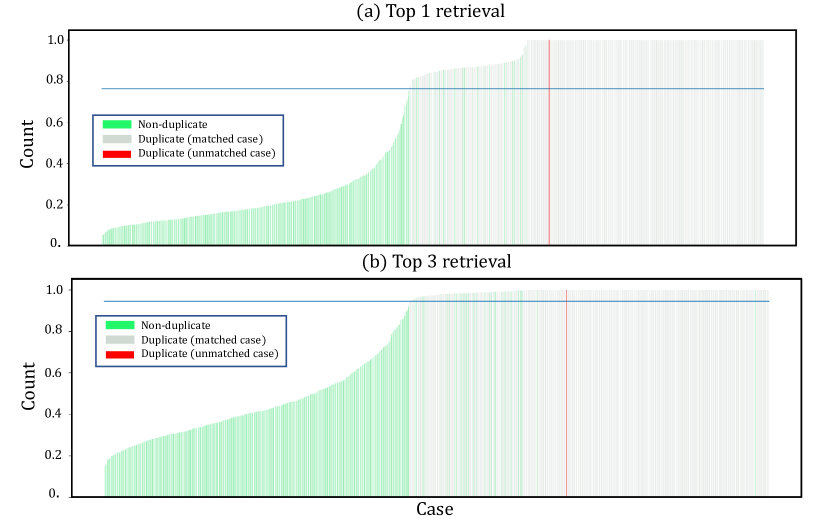
Figure 3: Case-level normalized counts of top 1 and top 3 predictions indexed with HNSW using DINOv1 embeddings. Green bars denote non-duplicate queries and gray and red bars denote duplicate queries. Red bars show duplicate queries in which the top 1 predictions are in the database but do not match the ground truth image case ID. The blue horizontal bar is the threshold resulting in the maximum sum of sensitivity and specificity.

IV-A2 Near-duplicate vs. Non-duplicate

Table III displays stage 1’s AUC of the top 3 retrievals indexed by HNSW and using DINOv1 embeddings. The ROC curves for top 1 with combinations of other indices and feature extractors follow the same tendency and hence are not shown. Under lowest strength, cropped, translated, noisy, and JPEG-compressed embeddings maintained AUC scores above 0.95, followed by rotation at 0.9327 and blurring at 0.9360. When stronger transformations were considered, all transformations showed an expected decrease in AUC scores proportional to the strength. At the strongest level, the AUC scores by blurring and Gaussian noise rose by a small margin compared to the preceded level. We postulated that under this range, the images are significantly altered and the embeddings are matched to non-informative slices of different volumes. Therefore even though the AUC scores seem to increase in stage 1, they show a consistent decrease in stage 2 where case IDs are matched (Table IV). Regarding the feature extractors, we observed a lower performance of DINOv2 compared to DINOv1 by a margin of 0.1-0.3 AUC. Nevertheless, the best and worst transformations are consistent between the two types of embeddings.

TABLE III: (Bucket 1B-1C, Stage 1) AUC of near-duplicates classification using DINOv1 embeddings with HNSW index for top 3 retrieval

Transform	Strength of transformation
Cropping	crop=5%	crop=10%	crop=15%	crop=20%
	0.9830	0.9618	0.8817	0.8024
Rotation	angle=5o	angle=10o	angle=15o	angle=20o
	0.9327	0.9053	0.8645	0.8426
Translation	shift=5%	shift=10%	shift=15%	shift=20%
	0.9619	0.9493	0.9388	0.9209
Blurring	sigma=1	sigma=2	sigma=4	sigma=8
	0.9360	0.7127	0.6916	0.7711
JPEG	quality=100%	quality=75%	quality=50%	quality=25%
compression	0.9821	0.9699	0.9405	0.8816
Gaussian	std=0.1	std=0.2	std=0.4	std=0.8
noise	0.9675	0.8437	0.6456	0.6789

TABLE IV: (Bucket 1B-1C, Stage 2) Sensitivity of near-duplicates classification using DINOv1 embeddings with HNSW index for top 3 retrieval

Transform	Strength of transformation
Cropping	crop=5%	crop=10%	crop=15%	crop=20%
	0.9942	0.9604	0.8161	0.6286
Rotation	angle=5o	angle=10o	angle=15o	angle=20o
	0.8778	0.8522	0.8300	0.8114
Translation	shift=5%	shift=10%	shift=15%	shift=20%
	0.9581	0.8708	0.8545	0.8510
Blurring	sigma=1	sigma=2	sigma=4	sigma=8
	0.8196	0.5239	0.1735	0.0163
JPEG	quality=100%	quality=75%	quality=50%	quality=25%
compression	0.9709	0.9267	0.8468	0.8102
Gaussian	std=0.1	std=0.2	std=0.4	std=0.8
noise	0.9779	0.8568	0.3050	0.0664

IV-A3 Selected optimal threshold

After observing the retrieval performance using buckets 1A, 1B, and 1C, which are presented in Table A.1, A.2, and A.3 of the Appendix, we decided to prioritize the top 3 retrievals using the HNSW index. Even though this choice slightly decreases specificity, it offers higher sensitivity as a trade-off. We determined $t_{opt}$ on the train set (Algorithm 1) with 7 query sets, including 6 near-duplicate query sets of the lowest transformation strength and 1 duplicate query set. The chosen $t_{opt}$ is 0.7711 and will be used to evaluate the detection performance using buckets 2A (duplicates), 2B (near-duplicates), and 2C (non-duplicates).

IV-B Evaluation with selected decision threshold

In Table V, we present the best sensitivity and specificity results for (near-) duplicate detection on buckets 2A, 2B, 2C using the top-3 retrievals obtained through DINOv1 embeddings with HNSW indexing. Overall, for stage 1, the mean sensitivity score is 0.9645, while for stage 2, it is 0.9407. In terms of mean specificity, we found scores of 0.8559 for stage 1 and 0.8373 for stage 2. Rotation exhibits the lowest sensitivity, mirroring trends observed in the training dataset. We also observed some false positive occurrences that are indeed in our database, which is due to the fact that possible identical images are shared among different MSD tasks. Upon scanning through 10 tasks, we were able to find 28 pairs of possible (near-) duplicates in the original MSD dataset shown in Table B.1. The majority of detected (near-) duplicates are from task 1, which contains the MRI brain images. An example is shown in Figure B.1 where two cases are different only in the brightness.

TABLE V: (Bucket 2A-2B-2C) Sensitivity and specificity using the threshold of 0.7711 for DINOv1 embeddings with HNSW index

	Sensitivity		Specificity
Transform	Stage 1	Stage 2	Stage 1	Stage 2
No transform (duplicate)	0.9977	0.9977	0.8559	0.8559
Cropping (crop=5%)	0.9865	0.9865	0.8559	0.8559
Translation (shift=5%)	0.9481	0.9481	0.8559	0.8559
Rotation (angle=5o)	0.8849	0.8826	0.8559	0.8539
Blurring (sigma=1)	0.9639	0.8442	0.8559	0.7646
JPEG (quality=100%)	0.9977	0.9549	0.8559	0.8207
Noise (std=0.1)	0.9729	0.9707	0.8559	0.8539
Mean	0.9645	0.9407	0.8559	0.8373

V Conclusion

In this study, we introduced and evaluated our approach for near- and duplicate detection of 3D medical images with pretrained vision embeddings. We tested its performance with near-duplicate queries involving different transformations and strengths. Through this, we established a process to find a single threshold value for balanced performance in both tasks. Our top results show 0.9645 sensitivity and 0.8559 specificity for detecting duplicates and near-duplicates with mild image transformations. This underscores the transferability of pretrained embeddings from natural images to medical imaging. Additionally, our method successfully pinpointed potential (near-) duplicates in MSD datasets, validating its effectiveness and emphasizing the importance of duplicate detection on datasets before experiments. We consider extending our study with naturally occurring near duplicates, e.g., same patient at different time points, as well as different volume sampling strategies to address spatial redundancy in future work.

Compliance with Ethical Standards

This research study was conducted retrospectively using human subject data made available in open access by https://medicaldecathlon.com/. Ethical approval was not required as confirmed by the license attached with the open access data.

Conflicts of Interest

No funding was received for conducting this study. The authors have no relevant financial or non-financial interests to disclose.

Appendix

V-A Near-duplicate detection results

We present in this section the full results of near-duplicate analysis on buckets 1A, 1B, and 1C. The evaluation was conducted using two feature extractors DINOv1 and DINOv2, and two database indices LSH and HNSW. For stage 1 (Table A.1), we report only AUC, and for stage 2, we report the sensitivity (Table A.2) and specificity (Table A.3) associated with $t_{ROC}$. For all metrics, we show the results with top-1 and top-3 retrieval.

TABLE A.1: (Bucket 1B-1C, Stage 1) AUC of near-duplicates classification using DINOv1 and DINOv2 embeddings with LSH and HNSW indexing. Left: top-1 retrieval. Right: top-3 retrieval

Transform	Strength	DINOv1		DINOv2
		LSH	HNSW	LSH	HNSW
Crop	crop=5%	0.9902	0.9887	0.9661	0.9732
	crop=10%	0.9751	0.9762	0.8964	0.9102
	crop=15%	0.8736	0.8932	0.7624	0.7835
	crop=20%	0.7876	0.7989	0.7190	0.7193
Rotation	angle=5o	0.9428	0.9457	0.9421	0.9461
	angle=10o	0.9156	0.9202	0.8864	0.8864
	angle=15o	0.8791	0.8775	0.8092	0.7912
	angle=20o	0.8576	0.8621	0.7225	0.6874
Translation	shift=5%	0.9688	0.9678	0.9675	0.9672
	shift=10%	0.9578	0.9577	0.9587	0.9580
	shift=15%	0.9474	0.9476	0.9482	0.9447
	shift=20%	0.9270	0.9290	0.9327	0.9273
Blurring	sigma=1	0.9385	0.9437	0.9008	0.8940
	sigma=2	0.7031	0.7164	0.6774	0.6529
	sigma=4	0.6330	0.6778	0.7456	0.6848
	sigma=8	0.7043	0.7534	0.8232	0.7470
	quality=100%	0.9820	0.9810	0.9830	0.9811
JPEG	quality=75%	0.9736	0.9741	0.9636	0.9618
Compression	quality=50%	0.9480	0.9504	0.9344	0.9247
	quality=25%	0.8745	0.8894	0.8422	0.8562
	std=0.1	0.9621	0.9681	0.9292	0.9380
Gaussian	std=0.2	0.8195	0.8485	0.7956	0.8020
noise	std=0.4	0.6069	0.6354	0.5976	0.5951
	std=0.8	0.6451	0.6571	0.6114	0.6248

Transform	Strength	DINOv1		DINOv2
		LSH	HNSW	LSH	HNSW
Crop	crop=5%	0.9579	0.9830	0.9351	0.9581
	crop=10%	0.9372	0.9618	0.8661	0.8807
	crop=15%	0.8528	0.8817	0.7622	0.7781
	crop=20%	0.7906	0.8024	0.7276	0.7282
Rotation	angle=5o	0.9579	0.9830	0.9351	0.9581
	angle=10o	0.9372	0.9618	0.8661	0.8807
	angle=15o	0.8528	0.8817	0.7622	0.7781
	angle=20o	0.7906	0.8024	0.7276	0.7282
Translation	shift=5%	0.9411	0.9619	0.9399	0.9593
	shift=10%	0.9278	0.9493	0.9260	0.9448
	shift=15%	0.9185	0.9388	0.9128	0.9293
	shift=20%	0.9013	0.9209	0.8970	0.9124
Blurring	sigma=1	0.9164	0.9360	0.8811	0.8817
	sigma=2	0.7005	0.7127	0.7013	0.6773
	sigma=4	0.6561	0.6916	0.7752	0.7267
	sigma=8	0.7191	0.7711	0.8515	0.7902
	quality=100%	0.9637	0.9821	0.9639	0.9841
JPEG	quality=75%	0.9474	0.9699	0.9385	0.9535
Compression	quality=50%	0.9185	0.9405	0.9038	0.9141
	quality=25%	0.8531	0.8816	0.8213	0.8328
	std=0.1	0.9329	0.9675	0.9015	0.9090
Gaussian	std=0.2	0.8002	0.8437	0.7696	0.7618
noise	std=0.4	0.6217	0.6456	0.6104	0.5814
	std=0.8	0.6573	0.6789	0.6296	0.6190

TABLE A.2: (Bucket 1B-1C, Stage 2) Sensitivity of near-duplicates classification using DINOv1 and DINOv2 embeddings with LSH and HNSW indexing. Left: top-1 retrieval. Right: top-3 retrieval

Transform	Strength	DINOv1		DINOv2
		LSH	HNSW	LSH	HNSW
Crop	crop=5%	0.9732	0.9208	0.9627	0.6321
	crop=10%	0.9464	0.9546	0.6764	0.7229
	crop=15%	0.7695	0.7637	0.4517	0.4319
	crop=20%	0.4843	0.5204	0.3504	0.3667
Rotation	angle=5o	0.8952	0.9371	0.9313	0.9348
	angle=10o	0.8359	0.8044	0.7416	0.5460
	angle=15o	0.7811	0.7765	0.2992	0.2794
	angle=20o	0.7625	0.7590	0.1746	0.1513
Translation	shift=5%	0.9488	0.9756	0.9418	0.9686
	shift=10%	0.9034	0.9395	0.8917	0.9139
	shift=15%	0.8685	0.9127	0.8417	0.8533
	shift=20%	0.8405	0.8591	0.8231	0.8300
Blurring	sigma=1	0.7998	0.7974	0.7509	0.7683
	sigma=2	0.3760	0.4144	0.1735	0.1921
	sigma=4	0.0861	0.3539	0.0442	0.0373
	sigma=8	0.0093	0.0035	0.0116	0.0023
	quality=100%	0.9383	0.9464	0.9302	0.9360
JPEG	quality=75%	0.9302	0.8941	0.8766	0.8091
Compression	quality=50%	0.8778	0.8941	0.8172	0.8149
	quality=25%	0.7870	0.8056	0.6973	0.7055
	std=0.1	0.9616	0.9325	0.8917	0.7322
Gaussian	std=0.2	0.7113	0.7474	0.6228	0.6403
noise	std=0.4	0.2701	0.2864	0.2375	0.2177
	std=0.8	0.0268	0.0326	0.0384	0.0349

Transform	Strength	DINOv1		DINOv2
		LSH	HNSW	LSH	HNSW
Crop	crop=5%	0.9942	0.9942	0.7322	0.7288
	crop=10%	0.9325	0.9604	0.6310	0.7159
	crop=15%	0.7800	0.8161	0.3935	0.3970
	crop=20%	0.5972	0.6286	0.3411	0.3283
Rotation	angle=5o	0.8731	0.8778	0.8417	0.8359
	angle=10o	0.8428	0.8522	0.5274	0.5320
	angle=15o	0.8161	0.8300	0.3143	0.3399
	angle=20o	0.8068	0.8114	0.2456	0.2212
Translation	shift=5%	0.9430	0.9581	0.8987	0.8941
	shift=10%	0.9010	0.8708	0.8568	0.8312
	shift=15%	0.8487	0.8545	0.7497	0.7718
	shift=20%	0.8428	0.8510	0.7485	0.8126
Blurring	sigma=1	0.8091	0.8196	0.6938	0.6868
	sigma=2	0.5704	0.5239	0.3120	0.2305
	sigma=4	0.1538	0.1735	0.0675	0.0477
	sigma=8	0.0256	0.0163	0.0221	0.0128
	quality=100%	0.9686	0.9709	0.9197	0.9616
JPEG	quality=75%	0.9499	0.9267	0.8789	0.8533
Compression	quality=50%	0.8440	0.8498	0.6985	0.6612
	quality=25%	0.7858	0.8102	0.5844	0.5390
	std=0.1	0.9837	0.9779	0.7811	0.4924
Gaussian	std=0.2	0.8207	0.8568	0.6286	0.4889
noise	std=0.4	0.2992	0.3050	0.2398	0.1665
	std=0.8	0.0640	0.0664	0.0629	0.0419

TABLE A.3: (Bucket 1B-1C, Stage 2) Specificity of near-duplicates classification using DINOv1 and DINOv2 embeddings with LSH and HNSW indexing. Left: top-1 retrieval. Right: top-3 retrieval.

Transform	Strength	DINOv1		DINOv2
		LSH	HNSW	LSH	HNSW
Crop	crop=5%	0.8679	0.9734	0.8885	0.9746
	crop=10%	0.8602	0.8467	0.8848	0.8693
	crop=15%	0.7659	0.8344	0.7991	0.8731
	crop=20%	0.4805	0.5306	0.6083	0.6434
Rotation	angle=5o	0.8061	0.7768	0.8352	0.8185
	angle=10o	0.8231	0.8925	0.8609	0.9109
	angle=15o	0.8754	0.8776	0.8851	0.8963
	angle=20o	0.8385	0.8441	0.8503	0.8534
Translation	shift=5%	0.8667	0.8345	0.8883	0.8603
	shift=10%	0.8576	0.8343	0.8730	0.8554
	shift=15%	0.8567	0.8364	0.8730	0.8534
	shift=20%	0.8557	0.8307	0.8720	0.8573
Blurring	sigma=1	0.7265	0.7072	0.8503	0.8486
	sigma=2	0.6660	0.6211	0.7151	0.6647
	sigma=4	0.3539	0.2916	0.4315	0.4114
	sigma=8	0.3241	0.3453	0.3725	0.4103
	quality=100%	0.8626	0.8344	0.8846	0.8613
JPEG	quality=75%	0.8525	0.8931	0.8814	0.9091
Compression	quality=50%	0.8348	0.8077	0.8642	0.8429
	quality=25%	0.7757	0.7598	0.8203	0.8190
	std=0.1	0.8534	0.9087	0.8834	0.9168
Gaussian	std=0.2	0.6831	0.6639	0.7895	0.7695
noise	std=0.4	0.2459	0.3225	0.4099	0.4854
	std=0.8	0.3956	0.3979	0.5412	0.5574

Transform	Strength	DINOv1		DINOv2
		LSH	HNSW	LSH	HNSW
Crop	crop=5%	0.9133	0.9133	0.9260	0.9272
	crop=10%	0.8694	0.8451	0.8798	0.8707
	crop=15%	0.8326	0.8466	0.8527	0.8711
	crop=20%	0.5804	0.6254	0.7112	0.7180
Rotation	angle=5o	0.8705	0.8590	0.8798	0.8890
	angle=10o	0.8555	0.8497	0.8738	0.8773
	angle=15o	0.8197	0.7968	0.8566	0.8472
	angle=20o	0.7569	0.7344	0.8121	0.7968
Translation	shift=5%	0.8705	0.8532	0.8809	0.8809
	shift=10%	0.8705	0.9017	0.8798	0.9121
	shift=15%	0.9168	0.9133	0.9295	0.9272
	shift=20%	0.9179	0.9110	0.9306	0.9249
Blurring	sigma=1	0.7351	0.7330	0.8611	0.8661
	sigma=2	0.4257	0.4990	0.5181	0.5772
	sigma=4	0.2776	0.3527	0.3580	0.4696
	sigma=8	0.2775	0.3183	0.3502	0.3959
	quality=100%	0.9211	0.9000	0.9256	0.9188
JPEG	quality=75%	0.8459	0.8740	0.8609	0.8915
Compression	quality=50%	0.8840	0.8819	0.8971	0.8982
	quality=25%	0.8083	0.8090	0.8412	0.8393
	std=0.1	0.8705	0.8971	0.8798	0.9109
Gaussian	std=0.2	0.6626	0.7050	0.7762	0.7910
noise	std=0.4	0.3152	0.3764	0.5063	0.5726
	std=0.8	0.4276	0.4423	0.5961	0.6657

V-B Detected (near-) duplicates in MSD dataset

We scanned through the MSD datasets using our proposed approach to detect near- and duplicates across tasks and train/test subsets. We used the DINOv1 embeddings indexed with HNSW and a threshold of 0.8. Any potential (near-) duplicate flagged by the algorithm was manually reviewed and confirmed. We presented in the tables below the case IDs that were flagged as (near-) duplicates and the subset to which they belong. Case ID 1 and Case ID 2 refer to the filenames of duplicate pairs in the dataset.

TABLE B.1: Detected (near-) duplicates in MSD dataset

Case ID 1	Subset	Case ID 2	Subset
BRATS_432	Train	BRATS_142	Train
BRATS_416	Train	BRATS_099	Train
BRATS_442	Train	BRATS_166	Train
BRATS_398	Train	BRATS_063	Train
BRATS_082	Train	BRATS_404	Train
BRATS_460	Train	BRATS_225	Train
BRATS_065	Train	BRATS_400	Train
BRATS_406	Train	BRATS_084	Train
BRATS_445	Train	BRATS_172	Train
BRATS_464	Train	BRATS_235	Train
BRATS_396	Train	BRATS_051	Train
BRATS_224	Train	BRATS_459	Train
BRATS_457	Train	BRATS_220	Train
BRATS_405	Train	BRATS_083	Train
BRATS_448	Train	BRATS_181	Train
BRATS_261	Train	BRATS_471	Train
BRATS_550	Train	BRATS_549	Train
BRATS_666	Train	BRATS_663	Train
BRATS_508	Train	BRATS_509	Train
BRATS_522	Train	BRATS_521	Train
BRATS_717	Test	BRATS_226	Train
BRATS_691	Test	BRATS_052	Train
BRATS_720	Test	BRATS_243	Train
BRATS_710	Test	BRATS_169	Train
BRATS_719	Test	BRATS_233	Train
BRATS_685	Test	BRATS_030	Train
BRATS_721	Test	BRATS_253	Train
BRATS_687	Test	BRATS_032	Train
BRATS_727	Test	BRATS_270	Train
BRATS_683	Test	BRATS_022	Train
BRATS_701	Test	BRATS_130	Train
BRATS_690	Test	BRATS_047	Train
BRATS_715	Test	BRATS_221	Train
BRATS_726	Test	BRATS_268	Train
BRATS_702	Test	BRATS_135	Train
BRATS_725	Test	BRATS_262	Train
BRATS_711	Test	BRATS_170	Train
BRATS_689	Test	BRATS_042	Train
BRATS_693	Test	BRATS_077	Train
BRATS_698	Test	BRATS_117	Train
BRATS_684	Test	BRATS_025	Train
BRATS_712	Test	BRATS_194	Train
BRATS_724	Test	BRATS_259	Train
BRATS_716	Test	BRATS_223	Train

Case ID 1	Subset	Case ID 2	Subset
BRATS_676	Test	BRATS_021	Train
BRATS_707	Test	BRATS_153	Train
BRATS_697	Test	BRATS_116	Train
BRATS_728	Test	BRATS_272	Train
BRATS_677	Test	BRATS_024	Train
BRATS_699	Test	BRATS_126	Train
BRATS_713	Test	BRATS_198	Train
BRATS_723	Test	BRATS_257	Train
BRATS_709	Test	BRATS_163	Train
BRATS_678	Test	BRATS_023	Train
BRATS_688	Test	BRATS_034	Train
BRATS_708	Test	BRATS_161	Train
BRATS_682	Test	BRATS_027	Train
BRATS_694	Test	BRATS_092	Train
BRATS_686	Test	BRATS_031	Train
BRATS_695	Test	BRATS_112	Train
BRATS_700	Test	BRATS_128	Train
BRATS_704	Test	BRATS_144	Train
BRATS_681	Test	BRATS_028	Train
BRATS_714	Test	BRATS_218	Train
BRATS_722	Test	BRATS_254	Train
BRATS_692	Test	BRATS_076	Train
BRATS_705	Test	BRATS_146	Train
BRATS_703	Test	BRATS_143	Train
BRATS_679	Test	BRATS_029	Train
BRATS_696	Test	BRATS_115	Train
BRATS_718	Test	BRATS_230	Train
liver_14	Train	liver_15	Train
liver_0	Train	liver_1	Train
liver_171	Train	liver_172	Train
liver_169	Train	liver_170	Train
liver_137	Test	liver_74	Train
hepaticvessel_265	Train	spleen_19	Train
hepaticvessel_286	Train	hepaticvessel_287	Train
hepaticvessel_376	Test	spleen_18	Train
hepaticvessel_045	Test	hepaticvessel_139	Train
spleen_1	Test	hepaticvessel_433	Train
spleen_32	Train	colon_041	Train
spleen_48	Train	colon_055	Train
spleen_7	Test	hepaticvessel_362	Train
pancreas_027	Test	pancreas_032	Train
pancreas_007	Test	pancreas_228	Train
colon_067	Test	spleen_59	Train
colon_071	Test	spleen_60	Train

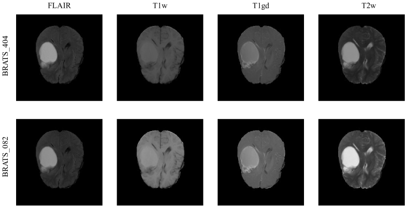
Figure B.1: Example of a near-duplicate found in MSD dataset. The BRATS_404 and BRATS_082 are a near-duplicate pair that is different only in the brightness.

References

- [1] D. G. Lowe, “Distinctive image features from scale-invariant keypoints,” International journal of computer vision, vol. 60, pp. 91–110, 2004.
- [2] H. Bay, T. Tuytelaars, and L. Van Gool, “Surf: Speeded up robust features,” in Computer Vision–ECCV 2006: 9th European Conference on Computer Vision, Graz, Austria, May 7-13, 2006. Proceedings, Part I 9. Springer, 2006, pp. 404–417.
- [3] Z. Zhou, K. Lin, Y. Cao, C.-N. Yang, and Y. Liu, “Near-Duplicate Image Detection System Using Coarse-to-Fine Matching Scheme Based on Global and Local CNN Features,” Mathematics, vol. 8, no. 4, p. 644, Apr. 2020, number: 4 Publisher: Multidisciplinary Digital Publishing Institute. [Online]. Available: https://www.mdpi.com/2227-7390/8/4/644
- [4] L. Morra and F. Lamberti, “Benchmarking unsupervised near-duplicate image detection,” Expert Systems with Applications, vol. 135, pp. 313–326, Nov. 2019, arXiv:1907.02821 [cs, stat]. [Online]. Available: http://arxiv.org/abs/1907.02821
- [5] T. Koker, S. Chintapalli, S. Wang, B. Talbot, D. Wainstock, M. Cicconet, and M. Walsh, “On Identification and Retrieval of Near-Duplicate Biological Images: a New Dataset and Protocol,” in 2020 25th International Conference on Pattern Recognition (ICPR). Milan, Italy: IEEE, Jan. 2021, pp. 3114–3121. [Online]. Available: https://ieeexplore.ieee.org/document/9412849/
- [6] Z. Zhou, Q. M. J. Wu, S. Wan, W. Sun, and X. Sun, “Integrating SIFT and CNN Feature Matching for Partial-Duplicate Image Detection,” IEEE Transactions on Emerging Topics in Computational Intelligence, vol. 4, no. 5, pp. 593–604, Oct. 2020. [Online]. Available: https://ieeexplore.ieee.org/document/9121754/
- [7] B. Barz and J. Denzler, “Do We Train on Test Data? Purging CIFAR of Near-Duplicates,” Journal of Imaging, vol. 6, no. 6, p. 41, Jun. 2020, number: 6 Publisher: Multidisciplinary Digital Publishing Institute. [Online]. Available: https://www.mdpi.com/2313-433X/6/6/41
- [8] K. He, X. Zhang, S. Ren, and J. Sun, “Deep residual learning for image recognition,” in Proceedings of the IEEE conference on computer vision and pattern recognition, 2016, pp. 770–778.
- [9] A. Dosovitskiy, L. Beyer, A. Kolesnikov, D. Weissenborn, X. Zhai, T. Unterthiner, M. Dehghani, M. Minderer, G. Heigold, S. Gelly et al., “An image is worth 16x16 words: Transformers for image recognition at scale,” arXiv preprint arXiv:2010.11929, 2020.
- [10] M. Caron, H. Touvron, I. Misra, H. Jégou, J. Mairal, P. Bojanowski, and A. Joulin, “Emerging properties in self-supervised vision transformers,” in Proceedings of the IEEE/CVF international conference on computer vision, 2021, pp. 9650–9660.
- [11] M. Oquab, T. Darcet, T. Moutakanni, H. Vo, M. Szafraniec, V. Khalidov, P. Fernandez, D. Haziza, F. Massa, A. El-Nouby et al., “Dinov2: Learning robust visual features without supervision,” arXiv preprint arXiv:2304.07193, 2023.
- [12] T. Truong, S. Mohammadi, and M. Lenga, “How transferable are self-supervised features in medical image classification tasks?” in Machine Learning for Health. PMLR, 2021, pp. 54–74.
- [13] M. Antonelli, A. Reinke, S. Bakas, K. Farahani, AnnetteKopp-Schneider, B. A. Landman, G. Litjens, B. Menze, O. Ronneberger, R. M. Summers, B. van Ginneken, M. Bilello, P. Bilic, P. F. Christ, R. K. G. Do, M. J. Gollub, S. H. Heckers, H. Huisman, W. R. Jarnagin, M. K. McHugo, S. Napel, J. S. G. Pernicka, K. Rhode, C. Tobon-Gomez, E. Vorontsov, H. Huisman, J. A. Meakin, S. Ourselin, M. Wiesenfarth, P. Arbelaez, B. Bae, S. Chen, L. Daza, J. Feng, B. He, F. Isensee, Y. Ji, F. Jia, N. Kim, I. Kim, D. Merhof, A. Pai, B. Park, M. Perslev, R. Rezaiifar, O. Rippel, I. Sarasua, W. Shen, J. Son, C. Wachinger, L. Wang, Y. Wang, Y. Xia, D. Xu, Z. Xu, Y. Zheng, A. L. Simpson, L. Maier-Hein, and M. J. Cardoso, “The Medical Segmentation Decathlon,” arXiv:2106.05735 [cs, eess], Jun. 2021, arXiv: 2106.05735. [Online]. Available: http://arxiv.org/abs/2106.05735
- [14] P. Virtanen, R. Gommers, T. E. Oliphant, M. Haberland, T. Reddy, D. Cournapeau, E. Burovski, P. Peterson, W. Weckesser, J. Bright, S. J. van der Walt, M. Brett, J. Wilson, K. J. Millman, N. Mayorov, A. R. J. Nelson, E. Jones, R. Kern, E. Larson, C. J. Carey, İ. Polat, Y. Feng, E. W. Moore, J. VanderPlas, D. Laxalde, J. Perktold, R. Cimrman, I. Henriksen, E. A. Quintero, C. R. Harris, A. M. Archibald, A. H. Ribeiro, F. Pedregosa, P. van Mulbregt, and SciPy 1.0 Contributors, “SciPy 1.0: Fundamental Algorithms for Scientific Computing in Python,” Nature Methods, vol. 17, pp. 261–272, 2020.
- [15] M. S. Charikar, “Similarity estimation techniques from rounding algorithms,” in Proceedings of the thiry-fourth annual ACM symposium on Theory of computing, 2002, pp. 380–388.
- [16] Y. A. Malkov and D. A. Yashunin, “Efficient and robust approximate nearest neighbor search using hierarchical navigable small world graphs,” IEEE transactions on pattern analysis and machine intelligence, vol. 42, no. 4, pp. 824–836, 2018.