Dual Structure-Preserving Image Filterings for Semi-supervised Medical Image Segmentation

Abstract

Semi-supervised image segmentation has attracted great attention recently. The key is how to leverage unlabeled images in the training process. Most methods maintain consistent predictions of the unlabeled images under variations (e.g., adding noise/perturbations, or creating alternative versions) in the image and/or model level. In most image-level variation, medical images often have prior structure information, which has not been well explored. In this paper, we propose novel dual structure-preserving image filterings (DSPIF) as the image-level variations for semi-supervised medical image segmentation. Motivated by connected filtering that simplifies image via filtering in structure-aware tree-based image representation, we resort to the dual contrast invariant Max-tree and Min-tree representation. Specifically, we propose a novel connected filtering that removes topologically equivalent nodes (i.e. connected components) having no siblings in the Max/Min-tree. This results in two filtered images preserving topologically critical structure. Applying such dual structure-preserving image filterings in mutual supervision is beneficial for semi-supervised medical image segmentation. Extensive experimental results on three benchmark datasets demonstrate that the proposed method significantly/consistently outperforms some state-of-the-art methods. The source codes will be publicly available.

1 Introduction

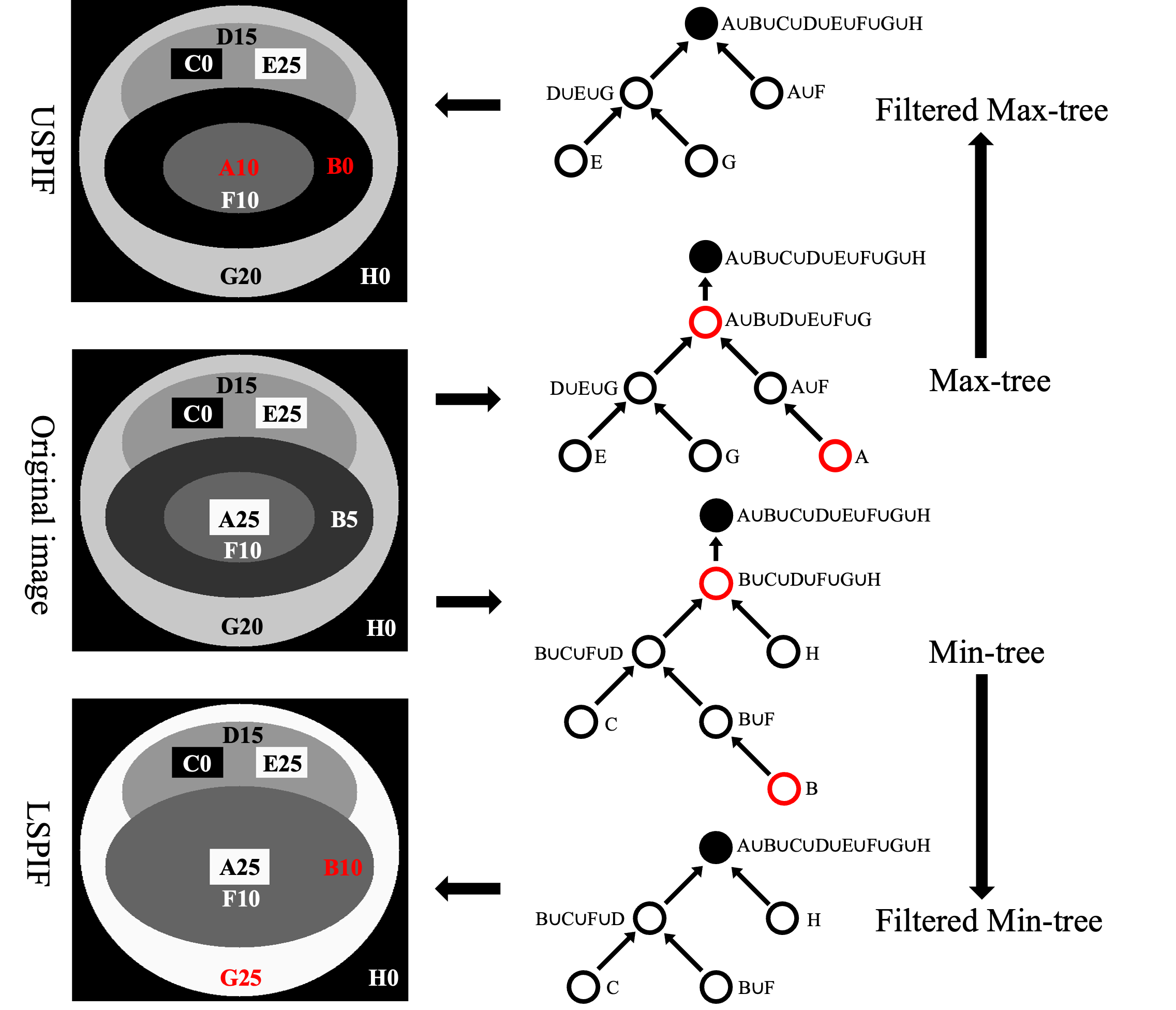
Figure 1: An illustrative example of the proposed DSPIF. For the Max-tree and Min-tree built on the original image, we remove every node (marked in red) without siblings which is topologically equivalent to its ancestor node. The two images reconstructed from filtered Max/Min-tree denoted as USPIF and LSPIF have the same topological structure as the original image, but are of quite different appearances. The number after the letter denotes the graylevel of the region.

Accurate medical image segmentation plays an important role in computer-aided diagnosis (CAD) systems. Traditional supervised segmentation methods have achieved impressive results using a large amount of labeled data. Yet, the manual segmentation is laborious and time-consuming. Recently, semi-supervised segmentation methods have gained significant attention by utilizing easily accessible unlabeled images to improve the accuracy of segmentation models.

The mainstream semi-supervised segmentation methods are based on consistency regularization [51, 33, 45, 4, 16, 14, 39, 5, 23], which aims to produce consistent results under variations at image-level or/and model-level. In particular, many approaches aim to generate variations under image-level [13, 41, 12, 27, 32]. A popular strategy for image variations utilizes the weak-to-strong paradigm [12, 20, 45], where predictions generated from weakly-augmented versions are used to supervise the strongly-augmented versions. Augmented versions are usually generated by simple random augmentation (e.g., Gaussian noise [13]), adversarial perturbation [27, 32], and CutMix techniques [10, 45]. The model-level variations mainly adopt the Mean Teacher framework [31] or Co-training strategy [29, 10]. In the Mean Teacher framework, the teacher network is usually obtained from the student network via Exponential Moving Average (EMA). The co-training strategy involves training two independent networks or decoders with different initializations and using each model’s outputs to supervise the other’s training in a mutual fashion.

Recently, the consistency regularization methods using pseudo labels for supervision have achieved impressive performance for semi-supervised segmentation [10, 45, 4, 23, 19]. For instance, CPS [10] generates different pseudo labels by two networks with different initializations and applies mutual supervision between them. These methods have achieved impressive performance in natural images, thanks to effective strong image augmentation (e.g., CutMix [49]) as image-level variations for avoiding the model overfit to incorrect pseudo-labels [10, 45, 20]. However, these existing image-level variations do not make well use of the structure information, which is important for medical images. Moreover, the distribution variance in medical images is not as significant as in natural images, which makes the semi-supervised medical image segmentation more prone to overfit noisy pseudo-labels due to confirmation bias [2].

We propose novel dual structure-preserving image filterings (DSPIF), serving as the image-level variations to cope with the confirmation bias in semi-supervised medical image segmentation. For that, we aim to obtain two filtered images with diverse image appearances while preserving the topological structure of the original image. Specifically, we resort to the dual contrast-invariant Max-tree and Min-tree [30] representation, given by the inclusion relationship between connected components of upper and lower level sets, respectively. The topology of the tree structure encodes the topology of the image structure. Such structure-aware tree-based image representation is widely used to implement connected filterings [30, 34, 35, 26, 44] that do not create new edges. We propose a novel type of connected filtering that preserves the topological structure of image. Precisely, we remove all nodes (i.e. connected components) having no siblings in the Max-tree and Min-tree, resulting in two simplified trees preserving topologically critical structure. The corresponding filters named upper/lower structure-preserving image filtering (denoted as USPIF and LSPIF) give rise to two different images having the same topological structure as the original image.

To further cope with the confirmation bias issue on unlabeled medical images, we also propose to apply monotonically increasing contrast changes before performing the dual structure-preserving image filterings. Since the Max-tree and Min-tree are invariant to such increasing changes, the resulting filtered images still preserve the topological structure while having large diversity in image appearances. Applying such dual structure-preserving image filterings as the image-level variations is beneficial for semi-supervised medical image segmentation. We adopt the mutual supervision framework of CPS [10] and MC-Net [36] as the baseline models. The proposed DSPIF significantly boosts the performance of CPS and MC-Net baseline, and significantly/consistently outperforms some state-of-the-art methods on three benchmark datasets.

The main contribution of the paper is summarized as follows: 1) We propose novel dual structure-preserving image filterings (DSPIF) as the image-level variations for semi-supervised medical image segmentation. DSPIF yields two images with quite different appearances while having the same topological structure as the original image. 2) We further leverage the contrast-invariance property of Max/Min-tree representation involved in DSPIF. We apply monotonically increasing contrast changes before performing DSPIF. This increases the appearance diversity while preserving topological image structure. 3) The proposed method significantly/consistently outperforms some state-of-the-art methods on three widely benchmark datasets. In particular, using only 20% of labeled images, the proposed method achieves similar ($\sim$99.5%) segmentation performance with the use of full dataset.

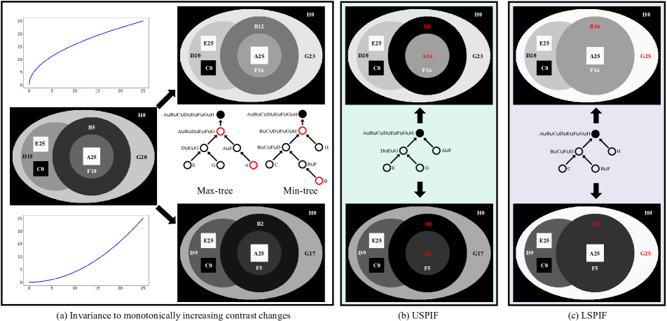
Figure 2: An illustrative example of leveraging the contrast-invariance property (a) of Max/Min-tree in DSPIF. Applying monotonically increasing contrast changes before DSPIF increases the appearance diversity while preserving the same topological structure as the original images.

2 Related work

2.1 Semi-supervised Medical Image Semantic Segmentation

Semi-supervised learning is widely used in medical image segmentation tasks thanks to its ability in alleviating the difficulty of manually annotating medical images. Methods [4, 16, 14, 39, 5, 33, 23] based on consistency regularization have achieved impressive performance for semi-supervised medical semantic segmentation. These methods usually use Mean Teacher framework [31] or Co-training strategy [29] to generate variations in the model-level. Another way aims to generate diverse versions of the same image and enforce prediction consistency under image variations [13, 41, 12, 27, 32]. A typical approach for image variations involves the weak-to-strong paradigm [12], where weakly-augmented and strongly-augmented images are employed to promote consistency. Methods [27, 32] incorporate adversarial training strategy to generate adversarial perturbations on images and make the predictions robust to adversarial perturbations. Recently, an increasing number of methods enhance model performance by training unlabeled images with pseudo labels [23, 28]. Since there are inevitable noisy labels in the pseudo labels for unlabeled images, it is crucial to determine the confidence level of pseudo-labels [28]. Moreover, some methods [20] focus on pseudo rectifying during the training stage. Considering that objects of interest in medical images have specific shapes, some works [17, 21, 24, 19] also incorporate shape information to alleviate the problem of insufficient labeled images in semi-supervised medical image segmentation. Li et al. [17] leverage signed distance map (SDM) of object surfaces and Luo et al. [21] use level set representations to capture geometric information of the target.

2.2 Tree-based image representation

Typically, an image is usually modeled as a discrete function defined on pixels or voxels over a 2D or 3D domain $V(\mathbb{R}^{2}\text{or}~{}\mathbb{R}^{3})$. However many applications rely on interacting with some primitives of fundamental elements being more meaningful than the pixels. The tree-based image representation [42, 44, 43] is composed of a set of regions of the original image. These regions are either disjoint or have inclusion relationship between them, and thus can be encoded into a tree structure. Hierarchical segmentation and threshold decomposition are two main branches of tree-based image representations. A hierarchy of segmentation consists of a set of fine to coarse partitions. This hierarchy can be depicted as a tree structure, with the root node representing the entire image as a unified region, and the leaf nodes denoting the regions within the finest image partition. The intermediate nodes, situated between the root and the leaves, represent regions obtained through the fusion of all the regions represented by their child nodes.

Threshold decompositions developed in mathematical morphology are another widely used type of tree-based image representation. This representation rely solely on pixel-value ordering, rendering the generated tree structures invariant to monotonically increasing contrast changes. Embedding the set of upper level sets into a tree structure gives the Max-tree [30]. The root of Max-tree represents the entire image domain, and the leaves correspond to the local regional maxima of the image. By duality, the lower level sets give rise to Min-tree representation [30]. The root of Min-tree also represents the entire image domain, while the leaves correspond to the local regional minima of the image. The Max/Min-tree can be computed with quasi-linear complexity based on Union-Find process [25, 9]. The tree structures constructed through threshold decomposition are all contrast-invariant, offering a multi-scale representation comprising a series of included or disjoint regions ranging from small to large scales [42, 44].

3 Method

3.1 Overview

Semi-supervised semantic segmentation task aims to enhance the performance of segmentation by leveraging a small set of labeled images $\mathcal{D}^{l}=\{(x^{l},y^{l})\}$ of $N$ labeled images, along with a large collection of unlabeled images $\mathcal{D}^{u}=\{x^{u}\}$ of $M$ unlabeled images, where $N\ll M$.

We follow classical consistency regularization-based semi-supervised medical image segmentation framework, which is often composed of image-level variations and model-level variations on unlabeled images. For the image-level variations, we resort to dual contrast-invariant Max-tree and Min-tree representation (see Sec. 3.2 for the construction) for connected filterings. We propose novel dual structure-preserving image filterings (DSPIF) as the image-level variations. More specifically, we propose a novel type of connected filtering that preserves only the topologically critical nodes of Max/Min-tree. The corresponding filtering named upper/lower structure-preserving image filtering denoted as USPIF/LSPIF, yields two different images that have the same topological structure as the original one. We further leverage the invariance property of Max/Min-tree with respect to monotonically increasing contrast changes to further enforce the appearance diversity while preserving the topological image structure. For the model variations, we simply adopt cross pseudo supervision (CPS) method [10] as a baseline example. The pipeline of the proposed framework is depicted in Supplementary. It is noteworthy that DSPIF can also be applied to other mutual supervision framework such as MC-Net [36].

3.2 Tree Construction

We utilize image threshold decompositions to build Max/Min-tree representation. By performing thresholding on a grayscale image $x$ in descending order, starting from $h_{max}$ to $h_{min}$, a sequence of nested upper level sets is obtained. Each upper level set at level $h$ is a binary image given by $\mathcal{X}_{h}(x)=\{v\in V|x(v)\geq h\}$. Let $P_{h}^{v}(x)$ represents the binary connected operator of $\mathcal{X}_{h}(x)$ at point $v$, which gives the connected component of $\mathcal{X}_{h}(x)$ containing $v$ if $v\in\mathcal{X}_{h}(x)$, and $\emptyset$ otherwise. Then, for any two connected components $P_{h_{1}}^{v_{1}}(x)$ and $P_{h_{2}}^{v_{2}}(x)$ at respectively level $h_{1}\geq h_{2}$, we have either $P_{h_{1}}^{v_{1}}(x)\subseteq P_{h_{2}}^{v_{2}}(x)$, or $P_{h_{1}}^{v_{1}}(x)\cap P_{h_{2}}^{v_{2}}(x)=\emptyset$. Based on this inclusion relationship, a tree structure named Max-tree is formed, where nodes correspond to connected components. The parenthood between nodes corresponds to the inclusion relationship between the underlying connected components.

We use a water-covered surface analogy to better illustrate the process of Max-tree construction and the associated alterations in the level sets. For that, we suppose the surface is entirely submerged in water. With the level of water gradually decreasing, islands (regional maxima) emerge first to form the leaves of the tree. As the water level continues to drop, these islands expand, building the tree’s branches. At certain levels, multiple islands fuse into a single connected piece, creating forks (i.e., the nodes of the tree with several children) in the tree structure. This process continues until all the water has evaporated, leaving behind a solitary landmass which forms the tree’s root, representing the entirety of the image. By duality, a corresponding dual structure of the Max-tree, known as the Min-tree, is constructed based on the decomposition of lower level sets defined by $\mathcal{X}^{h}(x)=\{v\in V|x(v)\leq h\}$. A synthetic example of Max-tree and Min-tree is given in Fig. 2(a). The Max/Min-tree can be constructed efficiently using Union-Find-based algorithms [25, 9], which has a quasi-linear complexity with respect to the number of pixels.

3.3 Dual Structure-Preserving Image Filterings

The Max/Min-tree representation is equivalent to the original image in the sense that the image $x$ can be reconstructed from the tree $\mathcal{T}$, composed of a set of nodes $\{\mathcal{N}\}$ with inclusion relationship encoded by $parent$. Specifically, we associate the graylevel $h$ to the corresponding node on which the underlying connected component is obtained. Then, for each pixel $v\in V$, the grayscale value $x(v)$ is given by the associated graylevel of the smallest node containing $v$. Removing nodes from the tree and updating the corresponding parenthood relationship results in a simplified tree, from which a filtered image is reconstructed. This is one of the most popular implementations of connected filters.

1

2 Function STRUCT_PRESERVE_FILTER($x$, $\tau$)

3       $\mathcal{T}$ $\leftarrow$ $Compute\_Tree$($x$)

4       foreach $\mathcal{N}\in\mathcal{T}$ do

5            $numChildren(\mathcal{N})\leftarrow 0$

6             $isRemoved(\mathcal{N})\leftarrow$ False

7      foreach $\mathcal{N}\in\mathcal{T}$ do

8             if $area(\mathcal{N})>\tau$ then

9                  $++numChildren(parent(\mathcal{N}))$

10            else

11                  $isRemoved(\mathcal{N})\leftarrow$ True

12      foreach $\mathcal{N}\in\mathcal{T}$ do

13             if $numChildren(parent(\mathcal{N}))=1$ then $isRemoved(\mathcal{N})\leftarrow$ True;

14            

15      foreach $v\in V$ do

16             $\mathcal{N}\leftarrow Get\_Node(v)$ //Smallest node contains $v$

17             while  $isRemoved(\mathcal{N})$ do

18                  $\mathcal{N}\leftarrow parent(\mathcal{N})$

19            $x^{\prime}(v)\leftarrow x(\mathcal{N})$

20      return $x^{\prime}$

Algorithm 1 Structure-preserving image filtering. Small regions with area less than $\tau$ may be caused by noise, and do not contribute to the topological changes.

The topology of the tree encodes the topology of the image structure. The leaf nodes correspond to local regional maxima (resp. minima) in the Max-tree (resp. Min-tree). A node having more than one child signifies the fusion of two connected components, triggering a topological change of tree structure and thus image structure. A node having no siblings is topologically equivalent to its parent. Therefore, removing all nodes having no siblings does not change the topological structure of the image. This gives a simplified tree preserving topologically critical nodes. The filtered image reconstructed from the simplified tree has the same topological structure as the original image, but with different appearances. Such filter $\psi$ is called upper/lower structure-preserving image filter denoted as USPIF and LSPIF for the use of Max-tree and Min-tree, respectively. Since the graylevel of the parent is smaller (resp. larger) than the graylevel of the current node in Max-tree (resp. Min-tree), the novel USPIF $\psi_{M}$ (resp. LSPIF $\psi_{m}$) actually belongs to the family of upper-leveling (resp. lower-leveling) [44]. The filtered image by USPIF is no brighter than the original image, and satisfies the property: for any pair of neighboring points $(v_{1},v_{2}):\psi_{M}(x)(v_{1})>\psi_{M}(x)(v_{2})\Rightarrow\psi_{M}(x)(v_{1})\leq x(v_{1})$. By duality, the filtered image by LSPIF is no darker than the original image and has the property: for any pair of neighboring points $(v_{1},v_{2}):\psi_{m}(x)(v_{1})>\psi_{m}(x)(v_{2})\Rightarrow\psi_{m}(x)(v_{2})\geq x(v_{2})$. An illustrative example of the proposed dual structure-preserving image filters (DSPIF) is given in Fig. 2(a).

The dual structure-preserving image filterings USPIF and LSPIF preserve the same topological structure as the original image while generating diverse image appearances different from the original one. It is noteworthy that different from classical monotonically increasing contrast changes (e.g., Gamma correction) where pixels with the same graylevel have the same output graylevel, the proposed DSPIF may yield different output graylevels for the same input graylevel (A and E regions from original image to USPIF in Fig. 1). Since small regions may be caused by noise, and do not contribute to the topological changes, we remove all nodes whose area is smaller than $\tau$ before performing DSPIF. The algorithm for the proposed strucutre-preserving image filtering is given in Algorithm 1.

Since the Max-tree and Min-tree are invariant to monotonically increasing contrast changes, we further increase the appearance diversity while preserving the topological structure by applying some monotonically increasing contrast changes to the original image before performing DSPIF. Specifically, we use Gamma correction or monotonic Bézier Curve for each training image. For the Gamma correction augmentations, we independently random two Gamma values within $[0.5,1.5]$ to generate two different views of the image. For Bézier curve augmentations, we use two end points ($P_{0}$ and $P_{3}$) and two control points ($P_{1}$ and $P_{2}$). We set $P_{0}=(-1,-1)$ and $P_{3}=(1,1)$ as fixed points. Then, we set $P_{1}=(-z,z)$ and $P_{2}=(z,-z)$, where $z\in[0,1]$. As illustrated in Fig. 2, applying such monotonically increasing contrast changes to the image before performing DSPIF yields many different alternatives with diverse appearances while preserving the topological structure of the original image.

3.4 Mutual Supervision on Dual Structure-Preserving Filtered Images

Network architecture: The model consists of two networks $f_{\theta_{1}}$ and $f_{\theta_{2}}$ with the same network architecture but different parameter initializations $\theta_{1}$ and $\theta_{2}$. For each image $x$, we apply the monotonically increasing contrast changes and the proposed DSPIF described in Sec. 3.3 to generate two different views $x_{1}$ and $x_{2}$ preserving the topological structure of the original image as the input for $f_{\theta_{1}}$ and $f_{\theta_{2}}$, respectively.

Training objective: For each labeled image $x^{l}$, we adopt the cross-entropy loss $\ell_{ce}$ and dice loss $\ell_{dc}$ as the supervised loss $\mathcal{L}_{s}$ given by:

$$\mathcal{L}_{s}=\ell_{ce}({p}_{1}^{l},{y}^{l})+\ell_{dc}({p}_{1}^{l},{y}^{l})+\ell_{ce}({p}_{2}^{l},{y}^{l})+\ell_{dc}({p}_{2}^{l},{y}^{l}),$$ (1)

where ${p}_{1}^{l}$ and ${p}_{2}^{l}$ are the prediction output of the two networks, and $y^{l}$ is the corresponding label. For each unlabeled image $x^{u}$, we use the pseudo label obtained from one network to supervise the output of another one. The loss $\mathcal{L}_{u}$ for the unlabeled image $x^{u}$ is given by:

$$\mathcal{L}_{u}=\ell_{ce}({p}_{1}^{u},\hat{y}_{2})+\ell_{ce}({p}_{2}^{u},\hat{y}_{1}),$$ (2)

where $\hat{y}_{1}$ and $\hat{y}_{2}$ are pseudo labels obtained from $p_{1}^{u}$ and $p_{2}^{u}$, respectively. The overall training objective $\mathcal{L}$ is defined by:

$$\mathcal{L}=\mathcal{L}_{s}+\lambda\times\mathcal{L}_{u},$$ (3)

where $\lambda$ balances the two loss terms.

4 Experiments

4.1 Dataset and Evaluation Protocal

Following some existing semi-supervised medical image semantic segmentation methods, we conduct experiments on three widely used datasets.

LA Dataset: 3D Left Atrial Segmentation Challenge dataset [40] consists of 100 MRI scans. Following Wu et al. [37], a fixed split is utilized, where 80 samples are designated for training and the remaining 20 samples are allocated for testing.

Pancreas-NIH Dataset: Pancreas-NIH dataset [11] consists of 82 3D abdominal contrast-enhanced CT scans. Following the commonly-used data split in Luo [21], we take 62 samples for training and the rest 20 samples for testing.

PROMISE12 Dataset: PROMISE12 dataset [18] consists of 50 transverse T2-weighted MRI scans. Following the data split in Liu et al. [19], there are 35, 5, and 10 scans for training, validation, and testing.

Evaluation protocol: The proposed method is evaluated with four widely used metrics in semi-supervised medical image segmentation: Dice coefficient (Dice), Jaccard Index (JAC), the 95% Hausdorff Distance (95HD), and the average surface distance (ASD).

4.2 Implementation Details

The SGD optimizer with a learning rate $10^{-2}$ and a weight decay factor $10^{-4}$ is used for all experiments. The loss weight $\lambda$ in Eq. (3) is set as a time-dependent Gaussian warming-up function [15] using the same parameters as MCNet+ [37]. We adopt the V-Net (resp. U-Net) model as the backbone for 3D (resp. 2D) segmentation tasks following the same settings in MC-Net+ [37]. All the experiments are conducted using the Pytorch framework with two NVIDIA GeForce RTX 4090 GPUs.

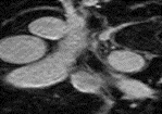
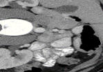
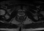
(a) Image

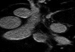
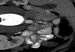
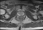
(b) Changed image

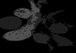
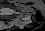
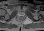
(c) USPIF

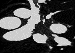
(d) LSPIF

Figure 3: Some qualitative results of DSPIF on LA dataset [40] (first row), Pancreas-CT [11] (middle row), and PROMISE12 [18] (bottom row). The changed images in (b) are obtained by applying monotonically increasing contrast change to the original ones.

4.3 Qualitative Results of DSPIF

Some qualitative results of the proposed DSPIF are shown in Fig. 3. Both USPIF and LSPIF generate images with diverse appearances while preserving the same topological structure as the original image. Inheriting from the property of connected filters, the proposed DSPIF does not create any new contours. It is also noteworthy that monotonically increasing contrast change map pixels with the same graylevel to the same output graylevel. Differently, the output of DSPIF does not only depend on the input graylevel, but also the image structure. As shown in the first row of Fig. 3, for similar input graylevels on different pixels, USPIF may output very different graylevels on these pixels. Yet, the topological image structure is preserved.

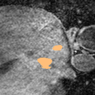
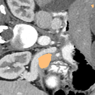
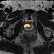
(a)

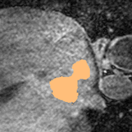
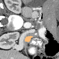
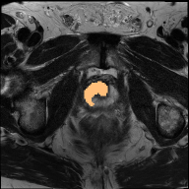
(b)

(c)

(d)

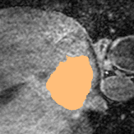
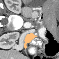
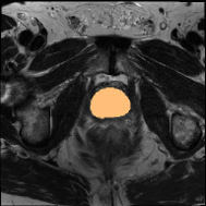
(e)

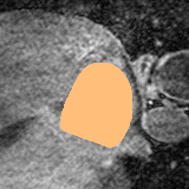
(f)

Figure 4: Some qualitative segmentation results on LA dataset [40] (first row), Pancreas-NIH dataset [11] (middle row), and PROMISE12 dataset [18] (bottom row).

4.4 Comparative Results on Different Datasets

Some qualitative segmentation results on the three datasets are shown in Fig. 4, where we can observe that the proposed DSPIF achieves accurate segmentation results.

Results on LA Dataset: Tab. 1 depicts the quantitative evaluation of the LA dataset. The proposed DSPIF achieves consistent improvement in terms of all four metrics compared with other state-of-the-art methods, achieving 90.63% and 91.63% Dice using 10% and 20% labeled data, respectively. Using 20% labeled data achieves $\sim$99.8% Dice performance of using full set of labeled data.

Table 1: Quantitative evaluation on the LA dataset [40]. † represents the reproduced results based on the open-sourced implementation. We report the mean and standard deviation obtained over three runs.

L/U	Method	Dice (%)$\uparrow$	JAC (%)$\uparrow$	95HD$\downarrow$	ASD$\downarrow$
80/0	V-Net†	91.82	84.92	5.12	1.71
8/0	V-Net†	80.75	69.81	15.11	3.61
8/72	CVRL [46]	88.56	78.89	8.22	2.81
(10%)	SS-Net [38]	88.55	79.62	7.49	1.90
	SimCVD [47]	89.03	80.34	8.34	2.59
	LLRU [1]	86.58	-	11.82	-
	MC-Net$+$ [37]	88.96	80.25	7.93	1.86
	BCP [3]	89.62	81.31	6.81	1.76
	MCNet [36]†	87.89$\pm$0.51	78.58$\pm$0.51	10.47$\pm$1.98	2.23$\pm$0.48
	MCNet + DSPIF	90.63$\pm$0.34	82.92$\pm$0.45	6.69$\pm$0.97	1.57$\pm$0.26
	CPS [10]†	86.79$\pm$0.42	77.05$\pm$0.56	14.19$\pm$2.08	4.25$\pm$0.40
	CPS + DSPIF	90.20$\pm$0.14	82.22$\pm$0.23	6.72$\pm$0.19	1.77$\pm$0.12
16/0	V-Net†	88.41	79.43	10.05	2.40
16/64	CVRL [46]	90.45	83.02	6.56	1.81
(20%)	SimCVD [47]	90.85	83.80	6.03	1.86
	LLRU [1]	88.60	-	7.61	-
	MC-Net$+$ [37]	91.07	83.67	5.84	1.67
	MCF [33]	88.71	80.41	6.32	1.90
	BCP [3]†	90.03	82.35	6.17	1.68
	MCNet [36]†	90.21$\pm$0.34	82.24$\pm$0.63	6.78$\pm$0.87	1.70$\pm$0.31
	MCNet + DSPIF	91.63$\pm$0.26	84.61$\pm$0.42	5.33$\pm$0.58	1.35$\pm$0.19
	CPS [10]†	90.07$\pm$0.30	82.08$\pm$0.49	6.81$\pm$0.41	1.99$\pm$0.21
	CPS + DSPIF	91.20$\pm$0.21	83.90$\pm$0.35	5.49$\pm$0.37	1.57$\pm$0.08

Results on Pancreas-NIH Dataset: The quantitative results on the Pancreas-NIH dataset are shown in Tab. 2. Under the setting of using 10% labeled images, the proposed DSPIF achieves consistent improvement in terms of all four metrics compared with other state-of-the-art methods, achieving 80.91% Dice, 68.31% JAC, 7.67 95HD, and 2.18 ASD. Using 20% labeled data under the CPS [10] baseline, the best result among our three experiments is 82.90 Dice, 71.10 JAC, and 1.60 ASD, which is comparable to the results of BCP [3].

Table 2: Quantitative evaluation on the Pancreas-NIH dataset [11].  † represents the reproduced results based on the open-sourced implementation. We report the mean and standard deviation obtained over three runs.

L/U	Method	Dice (%)$\uparrow$	JAC (%)$\uparrow$	95HD$\downarrow$	ASD$\downarrow$
62/0	V-Net†	82.68	71.05	5.19	1.41
6/0	V-Net†	68.69	55.03	13.47	3.63
6/56	UA-MT [48]	66.44	52.02	17.04	3.03
(10%)	URPC [22]	73.53	59.44	22.57	7.85
	DTC[21]	66.58	51.79	15.46	4.16
	MC-Net$+$ [37]	74.01	60.02	12.59	3.34
	BCP [3]†	75.57	61.35	27.29	8.16
	MCNet [36]†	69.47$\pm$0.82	55.28$\pm$1.15	20.74$\pm$1.98	5.41$\pm$0.67
	MCNet + DSPIF	70.49$\pm$0.84	56.63$\pm$1.27	13.03$\pm$2.12	2.48$\pm$0.84
	CPS [10]†	74.95$\pm$0.91	60.86$\pm$1.06	13.49$\pm$1.87	4.59$\pm$0.77
	CPS + DSPIF	80.91$\pm$0.70	68.31$\pm$0.92	7.67$\pm$1.63	2.18$\pm$0.25
12/0	V-Net†	76.91	63.86	8.16	2.07
12/50	UA-MT [48]	76.10	62.62	10.84	2.43
(20%)	URPC [22]	80.02	67.30	8.51	1.98
	DTC[21]	76.27	62.82	8.70	2.20
	CVRL[46]	76.68	61.16	8.24	3.19
	SimCVD [47]	75.39	61.56	9.84	2.33
	MC-Net$+$ [37]	80.59	68.08	6.47	1.74
	MCF [33]	75.00	61.27	11.59	3.27
	BCP [3]	82.91	70.79	6.43	2.25
	MCNet [36]†	78.26$\pm$0.35	65.12$\pm$0.42	11.90$\pm$2.04	3.25$\pm$0.83
	MCNet + DSPIF	79.13$\pm$0.42	66.23$\pm$0.38	7.77$\pm$1.65	1.85$\pm$0.43
	CPS [10]†	79.63$\pm$0.14	66.77$\pm$0.19	8.77$\pm$1.46	2.33$\pm$0.62
	CPS + DSPIF	82.66$\pm$0.32	70.75$\pm$0.44	7.11$\pm$1.01	1.75$\pm$0.22

Results on PROMISE12 Dataset: In Tab. 3, based on MCNet baseline, the proposed method achieves 24.0% Dice and 23.78% JAC (resp., 7.86% Dice and 8.16% JAC) improvement under the setting of using 10% (resp. 20%) labeled data. Compared with state-of-the-art method BCP [3], the proposed method built on CPS [10] achieves an improvement of 3.89% (resp. 3.73%) Dice when using 10% (resp. 20%) labeled data.

Table 3: Quantitative evaluation on the PROMISE12 dataset [18].  † represents the reproduced results based on the open-sourced implementation. We report the mean and standard deviation obtained over three runs.

L/U	Method	Dice (%)$\uparrow$	JAC (%)$\uparrow$	95HD$\downarrow$	ASD$\downarrow$
35/0	U-Net†	84.63	73.73	3.63	1.27
4/0	U-Net†	51.72	39.02	43.30	11.81
4/31	UA-MT [48]†	49.81	37.52	74.03	15.95
(10%)	URPC [22]†	51.70	38.30	75.19	22.32
	SALCC [19]†	63.85	48.07	40.68	7.50
	MC-Net$+$ [37]†	55.40	42.01	21.79	5.51
	SCP-Net [50]	66.21	-	-	11.56
	BCP [3]†	77.93	64.35	27.39	6.65
	MCNet [36]†	54.26$\pm$4.29	41.44$\pm$2.89	35.82$\pm$4.63	10.48$\pm$2.31
	MCNet + DSPIF	78.26$\pm$1.02	65.22$\pm$0.86	11.26$\pm$1.12	4.58$\pm$0.68
	CPS [10]†	63.55$\pm$2.50	48.08$\pm$1.76	40.50$\pm$2.66	12.20$\pm$1.42
	CPS + DSPIF	81.82$\pm$0.18	69.75$\pm$0.27	5.14$\pm$0.68	1.42$\pm$0.11
7/0	U-Net†	65.63	52.44	12.36	2.98
7/28	UA-MT [48]	61.55	-	-	13.94
(20%)	URPC [22]	61.55	-	-	9.63
	SALCC [19]	70.30	-	-	4.69
	MC-Net$+$ [37]†	66.91	55.26	12.74	2.41
	SCP-Net [50]	77.06	-	-	3.52
	BCP [3]†	80.26	67.46	9.67	4.87
	MCNet [36]†	71.70$\pm$1.26	59.71 $\pm$1.98	19.48$\pm$2.02	8.38$\pm$1.34
	MCNet + DSPIF	79.56$\pm$1.67	67.87$\pm$2.12	15.32$\pm$2.48	6.17$\pm$1.54
	CPS [10]†	72.06$\pm$2.73	59.53$\pm$2.21	9.55$\pm$1.72	1.71$\pm$0.05
	CPS + DSPIF	83.99$\pm$0.81	72.88$\pm$1.09	5.04$\pm$0.61	1.24$\pm$0.11

Table 4: Abaltion study on LA dataset [40]. We report the mean and standard deviation obtained over three runs.

CPS	Aug	DSPIF	Dice (%)	JAC (%)	95HD	ASD
✓			86.79$\pm$0.42	77.05$\pm$0.56	14.19$\pm$2.08	4.25$\pm$0.40
✓	✓		87.20$\pm$0.34	77.68$\pm$0.48	12.58$\pm$1.15	4.02$\pm$0.53
✓		✓	88.17$\pm$0.09	79.02$\pm$0.14	11.26$\pm$1.81	3.02$\pm$0.45
✓	✓	✓	90.20$\pm$0.14	82.22$\pm$0.23	6.72$\pm$0.19	1.77$\pm$0.12

Table 5: Ablation study on the area threshold $\tau$ involved in the proposed DSPIF on LA dataset [40].

Threshold $\tau$	0	50	100	150	200
Dice (%)	89.23	90.03	90.33	89.76	89.01

4.5 Ablation Studies

We conduct ablation studies on LA dataset under the setting of using 10% labeled data. As depicted in Tab. 4, directly adopting monotonically increasing contrast changes and random rotation as data augmentations do not significantly improve the results (86.79% to 87.20% Dice). Applying the proposed DSPIF on the original images outperforms the baseline by 1.38% Dice and 1.97% Jaccard index. Besides, combining these data augmentations and DSPIF significantly boosts the segmentation results by 3.0% Dice and 4.54% Jaccard index.

We also conduct an ablation study on the area threshold $\tau$ involved in the proposed DSPIF. As shown in Tab. 5, different settings of threshold $\tau$ slightly influence the results. Using too small values makes DSPIF sensitive to noise. Using too large values may filter out some important regions. Setting $\tau=100$ gives the best result.

4.6 Domain Generalization Results

Table 6: Cross-dataset performance on prostate segmentation. We report the mean and standard deviation over three runs.

Setting		L/U: 4/31		L/U: 7/28
		Dice (%)	JAC (%)	Dice (%)	JAC (%)
Site A	CPS (Baseline)	15.34$\pm$1.32	9.89$\pm$1.16	65.14$\pm$2.08	52.50$\pm$2.00
	CPS + Aug	28.80$\pm$5.39	18.73$\pm$4.02	70.43$\pm$2.33	57.31$\pm$1.29
	CPS + DSPIF	40.36$\pm$2.62	27.89$\pm$2.17	75.20$\pm$0.33	62.07$\pm$0.61
Site B	CPS (Baseline)	37.30$\pm$6.86	25.84$\pm$6.05	40.37$\pm$ 6.91	33.45$\pm$4.21
	CPS + Aug	39.89$\pm$1.84	28.10$\pm$1.69	55.14$\pm$2.97	41.03$\pm$1.00
	CPS + DSPIF	48.50$\pm$4.01	35.63$\pm$3.92	64.16$\pm$2.89	49.42$\pm$2.95

We conduct cross-domain experiments on prostate segmentation task in the semi-supervised setting to further verify the generalization performance of the proposed DSPIF. Under the setting of using 10% (resp. 20%) labeled data, we use 4 (resp. 7) labeled images and 31 (resp. 28) unlabeled images in PROMISE12 dataset to train the model, and test the model on 2 different data sources with distribution shift: Site A and B are from NCI-ISBI13 dataset [8]. As depicted in Tab. 6, though the monotonically increasing contrast changes is helpful in domain generalization, the proposed DSPIF further significantly improves the baseline of using monotonically increasing contrast changes, demonstrating the effectiveness of DSPIF in domain generalization under semi-supervised setting. Specifically, under the setting of using 10% labeled data, DSPIF achieves 11.56% (resp. 9.16%) Dice (resp. JAC) improvement on Site A and 8.61% (resp. 7.53%) Dice (resp. JAC) improvement on Site B. Under the setting of using 20% labeled data, DSPIF achieves 4.77% (resp. 4.76%) Dice (resp. JAC) improvement on Site A and a 9.02% (resp. 8.39%) Dice (resp. JAC) improvement on Site B.

4.7 Discussion

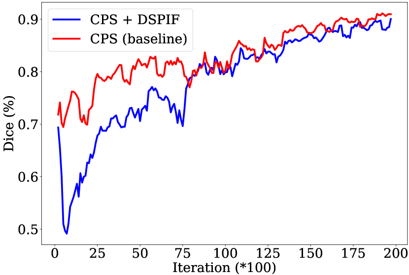
(a)

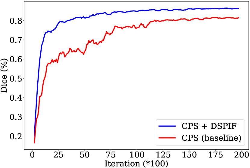
(b)

Figure 5: Dice Scores during training process on PROMISE12 Dataset [18]: (a) Erroneous predictions of two mutually supervised networks on unlabeled images, (b) Ground-truth and the network outputs on unlabeled images

The pseudo-label-based semi-supervised medical image segmentation methods focus on generating pseudo labels of high quality for unlabeled images. Since there are inevitable noisy labels in the pseudo labels for unlabeled images, it is critical to avoid the model overfitting to incorrect pseudo labels. Due to the absence of a clear supervision signal for the unlabeled image, when both networks make consistent incorrect predictions on some pixels, the mutual supervision between them may lead to a confirmation bias in the results. This makes the model overfit to noisy pseudo labels, yielding degenerated segmentation performance. Appropriate diversity between two networks’ erroneous predictions helps to avoid such confirmation bias issue of overfitting to incorrect pseudo-labels. We define a quantitative metric $D_{e}$ to characterize such diversity of erroneous predictions on unlabeled training images between the two mutually supervised networks. For that, let $\mathcal{E}^{1}$ and $\mathcal{E}^{2}$ denote the set of pixels with incorrect prediction of the first and second network, respectively. We compute $D_{e}$ as the Dice score between $\mathcal{E}^{1}$ and $\mathcal{E}^{2}$ given by $D_{e}=2\times|\mathcal{E}^{1}\cap\mathcal{E}^{2}|/(|\mathcal{E}^{1}|+|\mathcal{E}^{2}|).$ The comparison of $D_{e}$ for the baseline model and the proposed method during the training process is depicted in Fig. 5(a). Thanks to the large appearance diversity between USPIF and LSPIF while preserving the same topological structure as the original image, the proposed DSPIF has less consensus on the erroneous predictions of the two mutually supervised networks. This helps to alleviate the confirmation bias issue of overfitting to noisy pseudo labels on unlabeled images, resulting in better pseudo labels of unlabeled images during the training process (see Fig. 5(b)).

A limitation of the current work is that the proposed DSPIF requires some extra time during the training process (but no extra runtime during inference). The implementation of DSPIF mainly involves the construction of Max/Min-tree, which can be achieved in quasi-linear time complexity with respect to the number of pixels/voxels [25, 9]. Currently, we adopt CPU-based algorithm to build Max/Min-tree, which is not as efficient as GPU-based algorithm [7]. Yet, this GPU-based algorithm [7] does not support 3D images. In the future, we plan to explore the implementation of DSPIF with GPU to accelerate the training process. An alternative solution is to compute the DSPIF using offline strategy.

5 Conclusion

We propose a novel image-level variation method named dual structure-preserving image filterings (DSPIF) for semi-supervised medical image segmentation. Specifically, we leverage the dual Max-tree and Min-tree image representation, and remove all nodes having no siblings in the corresponding tree. This equals to remove all topologically equivalent regions while preserving topologically critical ones, resulting in two images with diverse appearances while having the same topological structure as the original image. Applying the proposed DSPIF to mutually supervised networks decreases the consensus of their erroneous predictions on unlabeled images. This helps to alleviate the confirmation bias issue of overfitting to noisy pseudo labels of unlabeled images, and thus effectively improves the segmentation performance. Extensive experimental results on three widely used benchmark datasets demonstrate that the proposed method significantly/consistently outperforms the state-of-the-art methods.

Supplementary Material

This supplementary material provides a more detailed introduction to the submitted manuscript from the following aspects. 6. The pipelines of DSPIF based on two baselines. 7.The detailed implementation of Max-tree and Min-tree. 8.Why Max-Tree and Min-tree are invariant to monotonically increasing contrast changes. 9.Ablation studies for hyper-parameters in monotonically increasing contrast changes.

6 The pipelines of DSPIF based on two baselines.

We incorporate the proposed DSPIF into two baselines, CPS [10] and MCNet [36], respectively. The pipeline of the proposed framework based on CPS [10] is depicted in Fig. 6. CPS [10] enforces consistency between two segmentation networks perturbed with distinct initializations while processing the same input image and employ the pseudo one-hot label map from one network to supervise the other network. DSPIF enables both networks to probabilistically receive images generated by either filtered Max-tree or filtered Min-tree in every iteration. When one network takes in an image generated using filtered Max-tree, the other network processes the same image generated with filtered Min-tree, and vice versa.

The pipeline of the proposed framework based on MCNet [36] is depicted in Fig. 7. MCNet [36] comprises one shared encoder and two different decoders with distinct up-sampling strategies. Different from CPS, MCNet [36] introduces a mutual consistency constraint between the probability output of one decoder and the soft pseudo labels of the other decoder. DSPIF enables the shared encoder to receive both Max-tree and Min-tree filtered images. The two decoders probabilistically receive features of images generated by either filtered Max-tree or filtered Min-tree in every iteration. When one decoder takes in features of the image generated with filtered Max-tree, the other decoder processes features of the same image generated with filtered Min-tree, and vice versa.

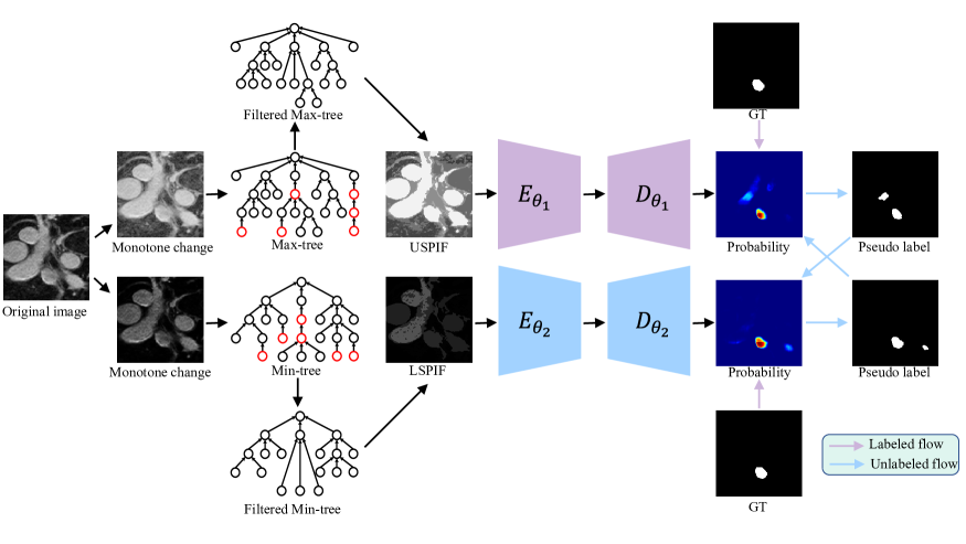
Figure 6: The pipeline of the proposed DSPIF framework using mutual supervision of CPS [10] as the model-level variations. The pipeline composed of image-level variations and model-level variations on images. We propose novel dual-structure preserving image filterings (DSPIF) based on Max/Min-tree representation as the image-level variations.

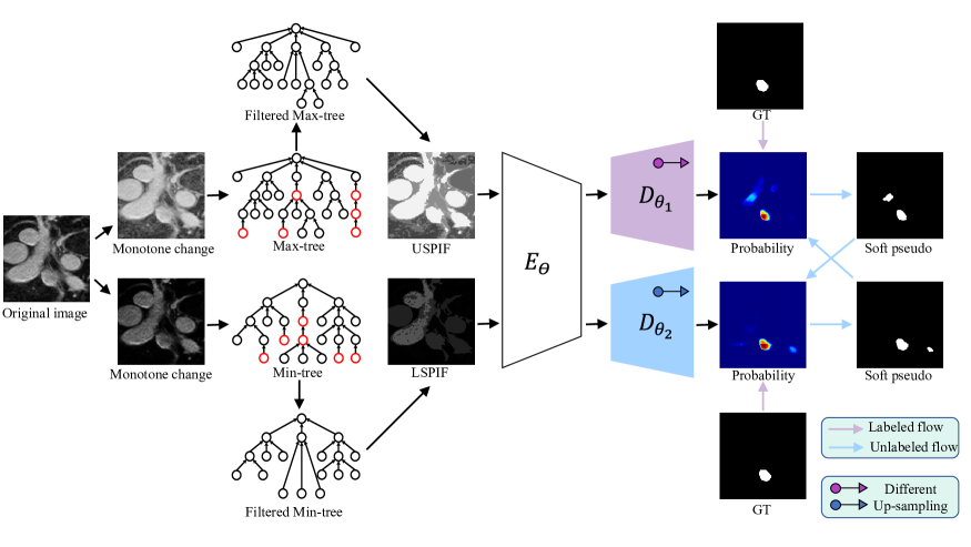
Figure 7: The pipeline of the proposed DSPIF framework using mutual supervision of MCNet [36] as the model-level variations. The pipeline composed of image-level variations and model-level variations on images. We propose novel dual-structure preserving image filterings (DSPIF) based on Max/Min-tree representation as the image-level variations.

7 The detailed implementation processes of Max-tree and Min-tree.

We use union-find method to efficiently compute the Max-tree and Min-tree [6, 30, 25, 9, 7]. It is composed of three steps given as follows:

1) When constructing the Max-tree, sort all pixels in the decreasing order. Inversely, sort all pixels in the increasing order when computing the Min-tree.

2) In the reverse order, use the union-find process to compute the ’correct’ tree.

3) Transform the ’correct’ tree to canonical Max-tree or Min-tree.

The union find algorithm is given in Algorithm. 2. The Max-tree and Min-tree construction algorithm is given in Algorithm. 3. For a better understanding of the algorithm, we demonstrate its steps through a simple synthetic image $x$ with size $2\times 5$ in Tab. 7.

// $\mathcal{R}$ : set of sorted pixels

// $N$ : total number of pixels

// $p,q,v$ : pixels

// $\Omega$ : neighbors

// $parent$ : image of parenthood

// $zpar$ : temporary parenthood

// $area$ : area of region

Input: An image $x$.

Output: Max-tree(Min-tree) of image $x$, areas of nodes.

1

2 Function FIND_ROOT($p$):

3       begin

4             if $zpar(p)=p$ then

5                  return $p$

6            else

7                  $zpar(p)\leftarrow\textnormal{{FIND\_ROOT(}}\textnormal{\emph{zpar(p)}}\textnormal{{)}}$;

8                   return $zpar(p)$

9 Function UNION_FIND($\mathcal{R}$):

10       begin

11             for  $p\in\mathcal{R}$ do

12                  $zpar(p)\leftarrow\text{undef}$;

13                   $area(p)\leftarrow 0$ ;

14                  

15            for  $i=N-1:0$ do

16                   $p\leftarrow\mathcal{R}[i]$;

17                   $parent(p)\leftarrow p$;

18                   $zpar(p)\leftarrow p$ ;

19                   $area(p)\leftarrow 1$ ;

20                   for  $q\in\Omega(p)\cap zpar(q)\neq undef$ do

21                         $v\leftarrow\textnormal{{FIND\_ROOT(}}\textnormal{\emph{q}}\textnormal{{)}}$;

22                         if $v\neq p$ then

23                               $parent(v)\leftarrow p$ ;

24                               $zpar(v)\leftarrow p$;

25                               $area(p)\leftarrow area(p)+area(v)$;

26                              

27            return $parent,area$

Algorithm 2 Union find algorithm.

// $\mathcal{R}$ : set of sorted pixels

// $N$ : total number of pixels

// $p,q$ : pixels

// $parent$ : image of parenthood

Input: An image $x$.

Output: Max-tree(Min-tree) of image $x$, areas of nodes.

1

2 Function CANONIZE_TREE($x$, $\mathcal{R}$, $parent$):

3       begin

4             for  $i=0:N-1$ do

5                   $p\leftarrow\mathcal{R}[i]$;

6                   $q\leftarrow parent(p)$;

7                   if $x(parent(q))=x(q)$ then

8                        $parent(p)\leftarrow parent(q)$ ;

9            return $parent$

10 Function COMPUTE_MIN_MAX_TREE($x$):

11       begin

12             $\mathcal{R}\leftarrow\textnormal{{SORT\_MONOTONE}}(x)$ ;

13             $parent,area\leftarrow$ UNION_FIND($\mathcal{R}$);

14             $parent\leftarrow$ CANONIZE_TREE(x, $\mathcal{R}$, parent);

15             return $parent,area$

Algorithm 3 Min-tree and Max-tree construction.

To construct the Min-tree, the initial step involves arranging the pixels in increasing order according to their grayscale values. The sorted pixels are displayed in Tab. 8. ’A’ represents the first element in the arrangement, ’B’ represents the second, and so forth. The result obtained after the initialization steps from lines 10 to 12 of the UNION_FIND in Algorithm. 2 is presented in Tab. 9. The results after each iteration of the $for$ loop from lines 13 to 24 in Algorithm. 2 are shown in Tab. 10 through Tab. 19. Concurrently, the corresponding Min-tree resulting from each iteration are depicted in Fig. 8 to Fig. 16. The tree in Fig. 16 is the ’correct’ tree. Tab. 20 represents the process of CANONIZE_TREE algorithm and Fig. 17 is the canonical Min-tree. The ’simplified tree’ obtained by merging pixels with parent-child relationships and identical grayscale values is displayed in Fig. 18. The ’simplified tree’ can be represented as Fig. 19, whose nodes symbolize areas in the image. The relationships between parent and child nodes denote the inclusion relationship between the regions. To compute the max-tree, it is sufficient to rearrange the pixel order in descending sequence.

Table 7: A simple synthetic image with size $2\times 5$.

2	2	4	1	3
1	4	3	2	4

Table 8: Increasing order of pixels according to grayscale values. ’A’ represents the first element in the arrangement.

2 (C)	2 (D)	4 (H)	1 (A)	3 (F)
1 (B)	4 (I)	3 (G)	2 (E)	4 (J)

Table 9: The result obtained after the initialization steps from lines 10 to 12 of the UNION_FIND algorithm .

Step 0	A	B	C	D	E
P($\cdot$)	$undef$	$undef$	$undef$	$undef$	$undef$
ZPar($\cdot$)	$undef$	$undef$	$undef$	$undef$	$undef$
Step 0	F	G	H	I	J
P($\cdot$)	$undef$	$undef$	$undef$	$undef$	$undef$
ZPar($\cdot$)	$undef$	$undef$	$undef$	$undef$	$undef$

Table 10: Results after 1 step of the $for$ loop from lines 13 to 24 in UNION_FIND algorithm.

Step 1	A	B	C	D	E
P($\cdot$)	A	$undef$	$undef$	$undef$	$undef$
ZPar($\cdot$)	A	$undef$	$undef$	$undef$	$undef$
Step 1	F	G	H	I	J
P($\cdot$)	$undef$	$undef$	$undef$	$undef$	$undef$
ZPar($\cdot$)	$undef$	$undef$	$undef$	$undef$	$undef$

Table 11: Results after 2 steps of the $for$ loop from lines 13 to 24 in UNION_FIND algorithm.

Step 2	A	B	C	D	E
P($\cdot$)	A	B	$undef$	$undef$	$undef$
ZPar($\cdot$)	A	B	$undef$	$undef$	$undef$
Step 2	F	G	H	I	J
P($\cdot$)	$undef$	$undef$	$undef$	$undef$	$undef$
ZPar($\cdot$)	$undef$	$undef$	$undef$	$undef$	$undef$

Figure 8: Tree structure obtained after 2 steps of the algorithm.

Table 12: Results after 3 steps of the $for$ loop from lines 13 to 24 in UNION_FIND algorithm.

Step 3	A	B	C	D	E
P($\cdot$)	A	C	C	$undef$	$undef$
ZPar($\cdot$)	A	C	C	$undef$	$undef$
Step 3	F	G	H	I	J
P($\cdot$)	$undef$	$undef$	$undef$	$undef$	$undef$
ZPar($\cdot$)	$undef$	$undef$	$undef$	$undef$	$undef$

Figure 9: Tree structure obtained after 3 steps of the algorithm.

Table 13: Results after 4 steps of the $for$ loop from lines 13 to 24 in UNION_FIND algorithm.

Step 4	A	B	C	D	E
P($\cdot$)	A	C	D	D	$undef$
ZPar($\cdot$)	A	C	D	D	$undef$
Step 4	F	G	H	I	J
P($\cdot$)	$undef$	$undef$	$undef$	$undef$	$undef$
ZPar($\cdot$)	$undef$	$undef$	$undef$	$undef$	$undef$

Figure 10: Tree structure obtained after 4 steps of the algorithm.

Table 14: Results after 5 steps of the $for$ loop from lines 13 to 24 in UNION_FIND algorithm.

Step 5	A	B	C	D	E
P($\cdot$)	E	C	D	D	E
ZPar($\cdot$)	E	C	D	D	E
Step 5	F	G	H	I	J
P($\cdot$)	$undef$	$undef$	$undef$	$undef$	$undef$
ZPar($\cdot$)	$undef$	$undef$	$undef$	$undef$	$undef$

Figure 11: Tree structure obtained after 5 steps of the algorithm.

Table 15: Results after 6 steps of the $for$ loop from lines 13 to 24 in UNION_FIND algorithm.

Step 6	A	B	C	D	E
P($\cdot$)	E	C	D	D	F
ZPar($\cdot$)	E	C	D	D	F
Step 6	F	G	H	I	J
P($\cdot$)	F	$undef$	$undef$	$undef$	$undef$
ZPar($\cdot$)	F	$undef$	$undef$	$undef$	$undef$

Figure 12: Tree structure obtained after 6 steps of the algorithm.

Table 16: Results after 7 steps of the $for$ loop from lines 13 to 24 in UNION_FIND algorithm.

Step 7	A	B	C	D	E
P($\cdot$)	E	C	D	D	F
ZPar($\cdot$)	E	C	D	D	F
Step 7	F	G	H	I	J
P($\cdot$)	G	G	$undef$	$undef$	$undef$
ZPar($\cdot$)	G	G	$undef$	$undef$	$undef$

Figure 13: Tree structure obtained after 7 steps of the algorithm.

Table 17: Results after 8 steps of the $for$ loop from lines 13 to 24 in UNION_FIND algorithm.

Step 8	A	B	C	D	E
P($\cdot$)	E	C	D	H	F
ZPar($\cdot$)	G	C	D	H	G
Step 8	F	G	H	I	J
P($\cdot$)	G	H	H	$undef$	$undef$
ZPar($\cdot$)	G	H	H	$undef$	$undef$

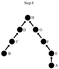
Figure 14: Tree structure obtained after 8 steps of the algorithm.

Table 18: Results after 9 steps of the $for$ loop from lines 13 to 24 in UNION_FIND algorithm.

Step 9	A	B	C	D	E
P($\cdot$)	E	C	D	H	F
ZPar($\cdot$)	G	H	I	H	G
Step 9	F	G	H	I	J
P($\cdot$)	G	H	I	I	$undef$
ZPar($\cdot$)	G	I	I	I	$undef$

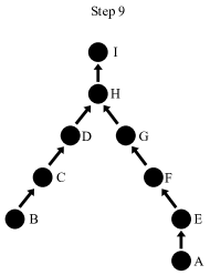
Figure 15: Tree structure obtained after 9 steps of the algorithm.

Table 19: Results after 10 steps of the $for$ loop from lines 13 to 24 in UNION_FIND algorithm.

Step 10	A	B	C	D	E
P($\cdot$)	E	C	D	H	F
ZPar($\cdot$)	G	H	I	H	I
Step 10	F	G	H	I	J
P($\cdot$)	G	H	I	J	J
ZPar($\cdot$)	J	J	I	J	J

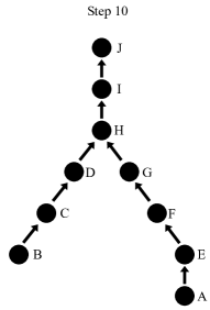
Figure 16: Tree structure obtained after 10 steps of the algorithm.

Table 20: The process of CANONIZE_TREE algorithm.

	$\xrightarrow{}$
$p$	J (4)	I (4)	H (4)	G (3)	F (3)
$q$	$\phi$	J (4)	I (4)	H (4)	G (3)
$P(q)$	$\phi$	$\phi$	J (4)	J (4)	J (4)
Change	$\phi$	$\phi$	$P$(H)=J	$P$(G)=J	$\phi$
	$\xrightarrow{}$
$p$	E (2)	D (2)	C (2)	B (1)	A (1)
$q$	F (3)	H (4)	D (2)	C (2)	E (2)
$P(q)$	G (3)	J (4)	J (4)	D (2)	G (3)
Change	$P$(E)=G	$P$(D)=J	$\phi$	$P$(B)=D	$\phi$

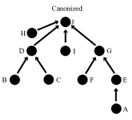
Figure 17: Tree structure obtained after canonized.

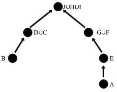
Figure 18: The ’simplified tree’ obtained by merging pixels with parent-child relationships and identical grayscale values.

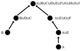
Figure 19: The ’simplified tree’ represented as a tree with inclusion relationship.

8 Why Max-Trees and Min-tree are invariant to monotonically increasing contrast changes.

When employing monotonically increasing contrast changes to adjust the image contrast, it does not alter the magnitude relationships between pixel grayscale values. Therefore, sorting pixels in ascending or descending order preserves their arrangement. As a result, monotonically increasing contrast changes does not affect the construction of the Max-tree and Min-tree. Tab. 21 and Tab. 22 illustrate this process.

Table 21: Employing monotonically increasing contrast changes to adjust the image contrast.

2	2	4	1	3
1	4	3	2	4
$\Downarrow$
4	4	8	2	6
2	8	6	4	8

Table 22: Increasing order of pixels after employing monotonically increasing contrast changes to adjust the image contrast.

2 (C)	2 (D)	4 (H)	1 (A)	3 (F)
1 (B)	4 (I)	3 (G)	2 (E)	4 (J)
$\Downarrow$
4 (C)	4 (D)	8 (H)	2 (A)	6 (F)
2 (B)	8 (I)	6 (G)	4 (E)	8 (J)

9 Ablation Studies for hyper-parameters in monotonically increasing contrast changes.

We use Gamma correction or monotonic Bézier Curve for each training image. Gamma correction controlled by $\gamma\in[a,b]$ to get augmented images $\hat{x}$ is given by:

$$\hat{x}=255*(\frac{x}{255})^{\gamma}$$ (4)

Based on CPS [10] baseline, We conducted an ablation experiment by varying the values of $a$ and $b$ on LA dataset [40] under the setting of using 10% labeled data. Tab. 23 shows that when $\gamma$ is randomly sampled from $[0.5,1.5]$, the best performance is achieved. $[1,1]$ represents not using Gamma correction, only utilizing Bézier curve as monotonically increasing contrast changes. Tab. 23 demonstrates that DSPIF is robust to $\gamma$, significantly improving the performance of the baseline across multiple parameter sets.

Table 23: Abaltion study on Gamma correction using LA dataset [40] under the setting of using 10% labeled data

$[a,b]$	Dice (%)	JAC (%)	95HD	ASD
CPS [10]	86.79	77.05	14.19	4.25
$[1,1]$	88.46	80.48	10.19	2.88
$[0.25,1.5]$	89.19	80.57	8.30	1.85
$[0.25,2]$	90.06	81.98	7.38	1.83
$[0.25,4]$	89.46	81.00	7.65	1.78
$[0.5,1.5]$	90.33	82.43	6.53	1.68
$[0.5,2]$	90.11	82.08	6.61	1.69
$[0.5,3]$	89.86	81.66	6.77	1.73
$[0.5,4]$	89.56	81.15	7.17	1.70

A Bézier curve is a parametric curve defined by a set of control points. In this paper, we use two end points ($P_{0}$ and $P_{3}$) and two control points ($P_{1}$ and $P_{2}$) to generate cubic Bézier curves $B(t)$:

$$B(t)=(1-t)^{3}P_{0}+3(1-t)^{2}tP_{1}+3(1-t)t^{2}P_{2}+t^{3}P_{3},~{}t\in[0,1],$$ (5)

where $t$ is a fractional value along the length of the line. We set $P_{0}=(-1,-1)$ and $P_{3}=(1,1)$ as fixed points. Then, we set $P_{1}=(-z,z)$ and $P_{2}=(z,-z)$. Using different values of $z$ yields distinct contrast transformation curves. Based on CPS [10] baseline, we conducted an ablation experiment on the range of values for $z$ using LA dataset under the setting of using 10% labeled data. $\phi$ in Tab. 24 represents not using Bézier curve, only utilizing Gamma correction as monotonically increasing contrast changes. When $z$ is randomly sampled from $\{0,0.5,0.75\}$, the best performance is achieved. Similar to $\gamma$, DSPIF is robust to $z$, significantly improving the performance of the baseline across multiple parameter sets.

Table 24: Abaltion study on Bézier curve using LA dataset [40] under the setting of using 10% labeled data

$z$	Dice (%)	JAC (%)	95HD	ASD
CPS [10]	86.79	77.05	14.19	4.25
$\phi$	89.77	81.51	6.79	1.75
$\{0,0.5\}$	90.03	81.94	6.65	1.77
$\{0,0.5,0.75\}$	90.33	82.43	6.53	1.68
$\{0,0.5,0.75,0.25\}$	89.64	81.30	7.25	1.81
$\{0,0.5,0.75,0.25,0.875\}$	89.43	80.96	7.39	1.87
$\{0,0.5,0.75,0.25,0.875,0.125\}$	89.56	81.16	7.73	1.93

References

- Adiga Vasudeva et al. [2022] Sukesh Adiga Vasudeva, Jose Dolz, and Herve Lombaert. Leveraging labeling representations in uncertainty-based semi-supervised segmentation. In Proc. of Int. Conf. Med. Image Comput. and Comput.-Assist. Intervent., pages 265–275, 2022.
- Arazo et al. [2020] Eric Arazo, Diego Ortego, Paul Albert, Noel E O’Connor, and Kevin McGuinness. Pseudo-labeling and confirmation bias in deep semi-supervised learning. In International Joint Conf. on Neural Networks, pages 1–8, 2020.
- Bai et al. [2023] Yunhao Bai, Duowen Chen, Qingli Li, Wei Shen, and Yan Wang. Bidirectional copy-paste for semi-supervised medical image segmentation. In IEEE Conf. Comput. Vis. Pattern Recog., pages 11514–11524, 2023.
- Basak and Yin [2023] Hritam Basak and Zhaozheng Yin. Pseudo-label guided contrastive learning for semi-supervised medical image segmentation. In IEEE Conf. Comput. Vis. Pattern Recog., pages 19786–19797, 2023.
- Basak et al. [2022] Hritam Basak, Sagnik Ghosal, and Ram Sarkar. Addressing class imbalance in semi-supervised image segmentation: A study on cardiac mri. In Proc. of Int. Conf. Med. Image Comput. and Comput.-Assist. Intervent., pages 224–233, 2022.
- Berger et al. [2007] Ch Berger, Th Géraud, Roland Levillain, Nicolas Widynski, Anthony Baillard, and Emmanuel Bertin. Effective component tree computation with application to pattern recognition in astronomical imaging. In IEEE Int. Conf. Image Process., pages IV–41, 2007.
- Blin et al. [2022] Nicolas Blin, Edwin Carlinet, Florian Lemaitre, Lionel Lacassagne, and Thierry Géraud. Max-tree computation on gpus. IEEE Transactions on Parallel and Distributed Systems, 33(12):3520–3531, 2022.
- Bloch et al. [2015] Nicholas Bloch, Anant Madabhushi, Henkjan Huisman, John Freymann, Justin Kirby, Michael Grauer, Andinet Enquobahrie, Carl Jaffe, Larry Clarke, and Keyvan Farahani. Nci-isbi 2013 challenge: automated segmentation of prostate structures. The Cancer Imaging Archive, 370:6, 2015.
- Carlinet and Géraud [2014] Edwin Carlinet and Thierry Géraud. A comparative review of component tree computation algorithms. IEEE Trans. Image Process., 23(9):3885–3895, 2014.
- Chen et al. [2021] Xiaokang Chen, Yuhui Yuan, Gang Zeng, and Jingdong Wang. Semi-supervised semantic segmentation with cross pseudo supervision. In IEEE Conf. Comput. Vis. Pattern Recog., pages 2613–2622, 2021.
- Clark et al. [2013] Kenneth Clark, Bruce Vendt, Kirk Smith, John Freymann, Justin Kirby, Paul Koppel, Stephen Moore, Stanley Phillips, David Maffitt, Michael Pringle, et al. The cancer imaging archive (TCIA): maintaining and operating a public information repository. Journal of Digital Imaging, 26(6):1045–1057, 2013.
- Fan et al. [2022] Jiashuo Fan, Bin Gao, Huan Jin, and Lihui Jiang. UCC: Uncertainty guided cross-head co-training for semi-supervised semantic segmentation. In IEEE Conf. Comput. Vis. Pattern Recog., pages 9947–9956, 2022.
- Huang et al. [2022] Wei Huang, Chang Chen, Zhiwei Xiong, Yueyi Zhang, Xuejin Chen, Xiaoyan Sun, and Feng Wu. Semi-supervised neuron segmentation via reinforced consistency learning. IEEE Trans. Medical Imaging., 41(11):3016–3028, 2022.
- Jin et al. [2022] Qiangguo Jin, Hui Cui, Changming Sun, Jiangbin Zheng, Leyi Wei, Zhenyu Fang, Zhaopeng Meng, and Ran Su. Semi-supervised histological image segmentation via hierarchical consistency enforcement. In Proc. of Int. Conf. Med. Image Comput. and Comput.-Assist. Intervent., pages 3–13, 2022.
- Laine and Aila [2016] Samuli Laine and Timo Aila. Temporal ensembling for semi-supervised learning. In Int. Conf. Learn. Represent., 2016.
- Lei et al. [2022] Tao Lei, Dong Zhang, Xiaogang Du, Xuan Wang, Yong Wan, and Asoke K Nandi. Semi-supervised medical image segmentation using adversarial consistency learning and dynamic convolution network. IEEE Trans. Medical Imaging., 2022.
- Li et al. [2020] Shuailin Li, Chuyu Zhang, and Xuming He. Shape-aware semi-supervised 3d semantic segmentation for medical images. In Proc. of Int. Conf. Med. Image Comput. and Comput.-Assist. Intervent., pages 552–561, 2020.
- Litjens et al. [2014] Geert Litjens, Robert Toth, Wendy van de Ven, Caroline Hoeks, Sjoerd Kerkstra, Bram van Ginneken, Graham Vincent, Gwenael Guillard, Neil Birbeck, Jindang Zhang, et al. Evaluation of prostate segmentation algorithms for MRI: the PROMISE12 challenge. Medical Image Analysis, 18(2):359–373, 2014.
- Liu et al. [2022a] Jinhua Liu, Christian Desrosiers, and Yuanfeng Zhou. Semi-supervised medical image segmentation using cross-model pseudo-supervision with shape awareness and local context constraints. In Proc. of Int. Conf. Med. Image Comput. and Comput.-Assist. Intervent., pages 140–150, 2022a.
- Liu et al. [2022b] Yuyuan Liu, Yu Tian, Yuanhong Chen, Fengbei Liu, Vasileios Belagiannis, and Gustavo Carneiro. Perturbed and strict mean teachers for semi-supervised semantic segmentation. In IEEE Conf. Comput. Vis. Pattern Recog., pages 4258–4267, 2022b.
- Luo et al. [2021a] Xiangde Luo, Jieneng Chen, Tao Song, and Guotai Wang. Semi-supervised medical image segmentation through dual-task consistency. In AAAI, pages 8801–8809, 2021a.
- Luo et al. [2021b] Xiangde Luo, Wenjun Liao, Jieneng Chen, Tao Song, Yinan Chen, Shichuan Zhang, Nianyong Chen, Guotai Wang, and Shaoting Zhang. Efficient semi-supervised gross target volume of nasopharyngeal carcinoma segmentation via uncertainty rectified pyramid consistency. In Proc. of Int. Conf. Med. Image Comput. and Comput.-Assist. Intervent., pages 318–329, 2021b.
- Lyu et al. [2022] Fei Lyu, Mang Ye, Jonathan Frederik Carlsen, Kenny Erleben, Sune Darkner, and Pong C Yuen. Pseudo-label guided image synthesis for semi-supervised covid-19 pneumonia infection segmentation. IEEE Trans. Medical Imaging., 42(3):797–809, 2022.
- Meng et al. [2022] Yanda Meng, Hongrun Zhang, Yitian Zhao, Dongxu Gao, Barbra Hamill, Godhuli Patri, Tunde Peto, Savita Madhusudhan, and Yalin Zheng. Dual consistency enabled weakly and semi-supervised optic disc and cup segmentation with dual adaptive graph convolutional networks. IEEE Trans. Medical Imaging., 42(2):416–429, 2022.
- Najman and Couprie [2006] Laurent Najman and Michel Couprie. Building the component tree in quasi-linear time. IEEE Trans. Image Process., 15(11):3531–3539, 2006.
- Ouzounis and Wilkinson [2007] Georgios K Ouzounis and Michael HF Wilkinson. Mask-based second-generation connectivity and attribute filters. IEEE Trans. Pattern Anal. Mach. Intell., 29(6):990–1004, 2007.
- Peiris et al. [2021] Himashi Peiris, Zhaolin Chen, Gary Egan, and Mehrtash Harandi. Duo-SegNet: adversarial dual-views for semi-supervised medical image segmentation. In Proc. of Int. Conf. Med. Image Comput. and Comput.-Assist. Intervent., pages 428–438, 2021.
- Qiao et al. [2022] Pengchong Qiao, Han Li, Guoli Song, Hu Han, Zhiqiang Gao, Yonghong Tian, Yongsheng Liang, Xi Li, S Kevin Zhou, and Jie Chen. Semi-supervised ct lesion segmentation using uncertainty-based data pairing and swapmix. IEEE Trans. Medical Imaging., 2022.
- Qiao et al. [2018] Siyuan Qiao, Wei Shen, Zhishuai Zhang, Bo Wang, and Alan Yuille. Deep co-training for semi-supervised image recognition. In Eur. Conf. Comput. Vis., pages 135–152, 2018.
- Salembier et al. [1998] Philippe Salembier, Albert Oliveras, and Luis Garrido. Antiextensive connected operators for image and sequence processing. IEEE Trans. Image Process., 7(4):555–570, 1998.
- Tarvainen and Valpola [2017] Antti Tarvainen and Harri Valpola. Mean teachers are better role models: Weight-averaged consistency targets improve semi-supervised deep learning results. Adv. Neural Inform. Process. Syst., 30, 2017.
- Wang et al. [2023a] Ping Wang, Jizong Peng, Marco Pedersoli, Yuanfeng Zhou, Caiming Zhang, and Christian Desrosiers. CAT: Constrained adversarial training for anatomically-plausible semi-supervised segmentation. IEEE Trans. Medical Imaging., 2023a.
- Wang et al. [2023b] Yongchao Wang, Bin Xiao, Xiuli Bi, Weisheng Li, and Xinbo Gao. MCF: Mutual correction framework for semi-supervised medical image segmentation. In IEEE Conf. Comput. Vis. Pattern Recog., pages 15651–15660, 2023b.
- Westenberg et al. [2007] Michel A Westenberg, Jos BTM Roerdink, and Michael HF Wilkinson. Volumetric attribute filtering and interactive visualization using the max-tree representation. IEEE Trans. Image Process., 16(12):2943–2952, 2007.
- Wilkinson et al. [2008] Michael HF Wilkinson, Hui Gao, Wim H Hesselink, Jan-Eppo Jonker, and Arnold Meijster. Concurrent computation of attribute filters on shared memory parallel machines. IEEE Trans. Pattern Anal. Mach. Intell., 30(10):1800–1813, 2008.
- Wu et al. [2021] Yicheng Wu, Minfeng Xu, Zongyuan Ge, Jianfei Cai, and Lei Zhang. Semi-supervised left atrium segmentation with mutual consistency training. In Proc. of Int. Conf. Med. Image Comput. and Comput.-Assist. Intervent., pages 297–306, 2021.
- Wu et al. [2022a] Yicheng Wu, Zongyuan Ge, Donghao Zhang, Minfeng Xu, Lei Zhang, Yong Xia, and Jianfei Cai. Mutual consistency learning for semi-supervised medical image segmentation. Medical Image Analysis, 81:102530, 2022a.
- Wu et al. [2022b] Yicheng Wu, Zhonghua Wu, Qianyi Wu, Zongyuan Ge, and Jianfei Cai. Exploring smoothness and class-separation for semi-supervised medical image segmentation. In Proc. of Int. Conf. Med. Image Comput. and Comput.-Assist. Intervent., pages 34–43, 2022b.
- Xiang et al. [2022] Jinyi Xiang, Peng Qiu, and Yang Yang. FUSSNet: Fusing two sources of uncertainty for semi-supervised medical image segmentation. In Proc. of Int. Conf. Med. Image Comput. and Comput.-Assist. Intervent., pages 481–491, 2022.
- Xiong et al. [2021] Zhaohan Xiong, Qing Xia, Zhiqiang Hu, Ning Huang, Cheng Bian, Yefeng Zheng, Sulaiman Vesal, Nishant Ravikumar, Andreas Maier, Xin Yang, et al. A global benchmark of algorithms for segmenting the left atrium from late gadolinium-enhanced cardiac magnetic resonance imaging. Medical Image Analysis, 67:101832, 2021.
- Xu et al. [2021] Xuanang Xu, Thomas Sanford, Baris Turkbey, Sheng Xu, Bradford J Wood, and Pingkun Yan. Shadow-consistent semi-supervised learning for prostate ultrasound segmentation. IEEE Trans. Medical Imaging., 41(6):1331–1345, 2021.
- Xu et al. [2014] Yongchao Xu, Pascal Monasse, Thierry Géraud, and Laurent Najman. Tree-based morse regions: A topological approach to local feature detection. IEEE Trans. Image Process., 23(12):5612–5625, 2014.
- Xu et al. [2016] Yongchao Xu, Edwin Carlinet, Thierry Géraud, and Laurent Najman. Hierarchical segmentation using tree-based shape spaces. IEEE Trans. Pattern Anal. Mach. Intell., 39(3):457–469, 2016.
- Xu, Yongchao and Géraud, Thierry and Najman, Laurent [2015] Xu, Yongchao and Géraud, Thierry and Najman, Laurent. Connected filtering on tree-based shape-spaces. IEEE Trans. Pattern Anal. Mach. Intell., 38(6):1126–1140, 2015.
- Yang et al. [2023] Lihe Yang, Lei Qi, Litong Feng, Wayne Zhang, and Yinghuan Shi. Revisiting weak-to-strong consistency in semi-supervised semantic segmentation. In IEEE Conf. Comput. Vis. Pattern Recog., pages 7236–7246, 2023.
- You et al. [2022a] Chenyu You, Ruihan Zhao, Lawrence H Staib, and James S Duncan. Momentum contrastive voxel-wise representation learning for semi-supervised volumetric medical image segmentation. In Proc. of Int. Conf. Med. Image Comput. and Comput.-Assist. Intervent., pages 639–652, 2022a.
- You et al. [2022b] Chenyu You, Yuan Zhou, Ruihan Zhao, Lawrence Staib, and James S Duncan. SimCVD: Simple contrastive voxel-wise representation distillation for semi-supervised medical image segmentation. IEEE Trans. Medical Imaging., 41(9):2228–2237, 2022b.
- Yu et al. [2019] Lequan Yu, Shujun Wang, Xiaomeng Li, Chi-Wing Fu, and Pheng-Ann Heng. Uncertainty-aware self-ensembling model for semi-supervised 3D left atrium segmentation. In Proc. of Int. Conf. Med. Image Comput. and Comput.-Assist. Intervent., pages 605–613, 2019.
- Yun et al. [2019] Sangdoo Yun, Dongyoon Han, Seong Joon Oh, Sanghyuk Chun, Junsuk Choe, and Youngjoon Yoo. CutMix: Regularization strategy to train strong classifiers with localizable features. In IEEE Conf. Comput. Vis. Pattern Recog., pages 6023–6032, 2019.
- Zhang et al. [2023] Zhenxi Zhang, Ran Ran, Chunna Tian, Heng Zhou, Xin Li, Fan Yang, and Zhicheng Jiao. Self-aware and cross-sample prototypical learning for semi-supervised medical image segmentation. In Proc. of Int. Conf. Med. Image Comput. and Comput.-Assist. Intervent., 2023.
- Zhao et al. [2023] Zhen Zhao, Lihe Yang, Sifan Long, Jimin Pi, Luping Zhou, and Jingdong Wang. Augmentation Matters: A simple-yet-effective approach to semi-supervised semantic segmentation. In IEEE Conf. Comput. Vis. Pattern Recog., pages 11350–11359, 2023.