Robust Bayesian graphical modeling using $\gamma$-divergence

Abstract

Gaussian graphical model is one of the powerful tools to analyze conditional independence between two variables for multivariate Gaussian-distributed observations. When the dimension of data is moderate or high, penalized likelihood methods such as the graphical lasso are useful to detect significant conditional independence structures. However, the estimates are affected by outliers due to the Gaussian assumption. This paper proposes a novel robust posterior distribution for inference of Gaussian graphical models using the $\gamma$-divergence which is one of the robust divergences. In particular, we focus on the Bayesian graphical lasso by assuming the Laplace-type prior for elements of the inverse covariance matrix. The proposed posterior distribution matches its maximum a posteriori estimate with the minimum $\gamma$-divergence estimate provided by the frequentist penalized method. We show that the proposed method satisfies the posterior robustness which is a kind of measure of robustness in the Bayesian analysis. The property means that the information of outliers is automatically ignored in the posterior distribution as long as the outliers are extremely large, which also provides theoretical robustness of point estimate for the existing frequentist method. A sufficient condition for the posterior propriety of the proposed posterior distribution is also shown. Furthermore, an efficient posterior computation algorithm via the weighted Bayesian bootstrap method is proposed. The performance of the proposed method is illustrated through simulation studies and real data analysis.

Keywords: Bayesian lasso; Gaussian graphical model; $\gamma$-divergence; posterior robustness; weighted Bayesian bootstrap

Introduction

Estimating the dependence structure between variables is an important issue in multivariate analysis. Let $y_{1},\dots,y_{n}$ be a sequence of independent, identically distributed random vectors according to the $p$-dimensional multivariate Gaussian distribution:

$$y_{i}\sim N_{p}(0,\Omega^{-1}),\quad i=1,\dots,n,$$ (1)

where $y_{i}=(y_{i1},\dots,y_{ip})^{\top}\in\mathbb{R}^{p}$ for $i=1,\dots,n$, and $\Omega=(\omega_{ij})\in\mathbb{R}^{p\times p}$ is a precision matrix defined by the inverse covariance matrix. The estimation of the precision matrix $\Omega$ under the Gaussian assumption is called the Gaussian graphical model (Lauritzen, 1996; Whittaker, 2009). Estimating the conditional dependence structures among variables corresponds to estimating whether the off-diagonals of the precision matrix are zero or not. To deal with the sparsity of the precision matrix, the penalized approach such as graphical lasso has been considered (e.g. Yuan and Lin, 2007; Friedman et al., 2008). The graphical lasso estimate is defined by minimizing the penalized log-likelihood

$$-\log|\Omega|+\mathrm{tr}(S\Omega)+\rho\|\Omega\|_{1}$$

over the space of positive definite matrices $M^{+}$. Note that $S=y^{\top}y/n$ is the sample covariance matrix, $\rho\geq 0$ is a tuning parameter, and $\|\Omega\|_{1}=\sum_{1\leq i,j\leq p}|\omega_{ij}|$. Friedman et al. (2008) proposed an efficient optimization algorithm, which guarantees symmetry and positive definiteness. Although the method provides the point estimates quickly, we cannot conduct a full probabilistic inference for the parameter of interest $\Omega$ in graphical models.

On the other hand, the Bayesian approach is useful for quantifying the uncertainty of the parameter of interest. As a Bayesian alternative to the graphical lasso, Wang (2012) proposed a Bayesian graphical lasso model defined by

$$y_{i}\mid\Omega \sim N_{p}(0,\Omega^{-1}),\quad i=1,\dots,n$$

$$\Omega\mid\lambda \sim C_{\lambda}^{-1}\prod_{i<j}\mathrm{Lap}(w_{ij}\mid\lambda)\prod_{i=1}^{p}\mathrm{Exp}\left(w_{ii}\mid\frac{\lambda}{2}\right)1_{\Omega\in M^{+}},$$

where $C_{\lambda}=\int\prod_{i<j}\mathrm{Lap}(w_{ij}\mid\lambda)\prod_{i=1}^{p}\mathrm{Exp}\left(w_{ii}\mid\frac{\lambda}{2}\right)1_{\Omega\in M^{+}}d\Omega$ is the normalizing constant of the prior density, and $\lambda>0$ is a prior hyper-parameter that plays the same role as the penalty parameter in the original graphical lasso. $\mathrm{Lap}(\cdot\mid\lambda)$ represents the Laplace (or double-exponential) density function of the form $\mathrm{Lap}(x\mid\lambda)=(\lambda/2)\exp(-\lambda|x|)$, and $\mathrm{Exp}(\cdot\mid\lambda)$ represents the exponential density function of the form $\mathrm{Exp}(x\mid\lambda)=\lambda\exp(-\lambda x)1_{x>0}$. The prior for $\Omega\mid\lambda$ is called the graphical lasso prior in Wang (2012). The Bayesian approach enables us to quantify the uncertainty through posterior credible intervals calculated by the posterior sample. Wang (2012) also proposed an efficient block Gibbs sampler to obtain the posterior sample. However, there is a drawback that the estimate of $\omega_{ij}$ for $i\neq j$ cannot be exactly zero, so we may need to consider a criterion to specify dependent structures.

However, these Gaussian graphical models can not lead to suitable estimates if the data involve outliers or data generating distribution is heavily-tailed. One of the remedies is to use a heavy-tailed multivariate distribution such as the multivariate $t$-distribution (see e.g. Finegold and Drton, 2011). However, as pointed out by Hirose et al. (2017), the heavy-tailed distribution generates both large and small outliers, and the variance of the estimator tends to be large. To overcome these issues, we consider the robust divergence to estimate Gaussian graphical models in the presence of outliers. In a frequentist perspective, Hirose et al. (2017) proposed the $\gamma$-lasso that is a robust estimation method of the inverse covariance matrix based on the $\gamma$-divergence (Fujisawa and Eguchi, 2008). Although the density-power divergence (Basu et al., 1998) is often used, it is known that the method does not work very much for the estimation of variance or scale parameter. Robust Bayesian modeling based on the $\gamma$-divergence has also been developed in recent years. For example, Hashimoto and Sugasawa (2020) proposed a robust and sparse Bayesian linear regression model, and Momozaki and Nakagawa (2023) considered a robust ordinal response model via the $\gamma$-divergence.

In this paper, we propose a robust Bayesian graphical lasso based on the $\gamma$-divergence. Although the proposed method combines the $\gamma$-lasso by Hirose et al. (2017) with the Bayesian graphical lasso by Wang (2012), we prove the robustness property called the posterior robustness for the proposed method. The posterior robustness is one of the robustness properties for posterior distributions. For the posterior distribution equipped with the property, the information of outliers is automatically rejected in the posterior distribution as long as the outliers are extremely large. Recently, some researchers studied sufficient conditions for the posterior robustness using log-regularly varying tailed probability distributions for data (Desgagné, 2015; Desgagné and Gagnon, 2019; Hamura et al., 2022). However, the posterior robustness for divergence-based robust methods has not been much developed. To show the posterior robustness under the $\gamma$-divergence, we introduce a new robust posterior distribution whose maximum a posteriori estimate matches the estimate by $\gamma$-lasso (Hirose et al., 2017). Since the proposed posterior distribution is a synthetic one, we provide a sufficient condition for the posterior propriety in the use of the Bayesian lasso-type priors. We also show that the other popular approaches do not satisfy the posterior robustness for the estimation of the inverse covariance matrix. We illustrate the performance of the proposed method through some numerical experiments, and we apply the proposed method to the analysis of gene expression data.

The remaining of the paper is structured as follows: In Section 2, a new robust posterior distribution based on the $\gamma$-divergence is proposed, and some theoretical properties and an efficient posterior computation algorithm are also presented. In Section 3, we discuss robustness properties for other posterior distributions. Numerical experiments and the real data example are shown in Sections 4 and 5, respectively. R code implementing the proposed methods is available at the GitHub repository (URL: https://github.com/Takahiro-Onizuka/RBGGM-gamma)

Robust Bayesian graphical models

In this section, we present our main proposal and show some theoretical properties of the proposed model. Furthermore, we provide an efficient and scalable posterior computation algorithm using a weighted Bayesian bootstrap.

Graphical lasso in the presence of outliers

It is well-known that parameter estimation under the Gaussian likelihood is affected by outliers. Studies on robust parameter estimation have a long history and many useful methods were proposed in the literature. One of the methods is to use heavy-tailed probability distribution instead of Gaussian distribution. For example, Finegold and Drton (2011) proposed a robust graphical lasso based on the multivariate $t$-distribution. However, constructing such a distribution equipped with desirable robustness properties is not straightforward, especially in multivariate cases. As a more versatile approach, divergence-based or weighted likelihood methods have been developed in the last two decades (see e.g. Basu et al., 1998). In this paper, we focus on a robust divergence called $\gamma$-divergence (Fujisawa and Eguchi, 2008). Hirose et al. (2017) considered a robust Gaussian graphical modeling based on the $\gamma$-divergence. The $\gamma$-divergence between a data generating process $g(y)$ and probability density function $f(y\mid\theta)$ is defined by

$$d_{\gamma}(g,f)=\frac{1}{\gamma(1+\gamma)}\log\int g(y)^{\gamma}dy-\frac{1}{\gamma}\log\int g(y)f(y\mid\theta)^{\gamma}dy+\frac{1}{1+\gamma}\log\int f(y\mid\theta)^{1+\gamma}dy,$$

where $\gamma>0$ is a tuning parameter to control the balance between efficiency and robustness. The selection method of $\gamma>0$ has been not clear in general, but some strategies have been developed in recent years (see e.g. Yonekura and Sugasawa, 2023). Throughout the paper, we fix $\gamma$ as a small positive value in numerical experiments. Since $g(y)$ is unknown in practice, the minimum $\gamma$-divergence estimate is obtain by solving the following optimization problem:

$$\min_{\theta}\left\{-\frac{1}{\gamma}\log\left\{\frac{1}{n}\sum_{i=1}^{n}f(y_{i}\mid\theta)^{\gamma}\right\}+\frac{1}{1+\gamma}\log\int f(y\mid\theta)^{1+\gamma}dy\right\}.$$ (2)

The objective function in (2) is also called the negative $\gamma$-likelihood function. Combining the $\gamma$-likelihood with $L_{1}$-penalty, Hirose et al. (2017) proposed a robust and sparse graphical lasso model. In the following sections, we consider the robust graphical lasso models in the Bayesian perspective.

MAP $\gamma$-posterior distribution

Robust Bayesian modeling via the $\gamma$-divergence has been developed in recent years (see Nakagawa and Hashimoto, 2020; Hashimoto and Sugasawa, 2020). Although the existing studies deal with robust Bayesian inference for univariate observations and linear regression models, we here focus on robust Bayesian inference for a precision matrix in multivariate Gaussian-distributed observations. To this end, we introduce a robust posterior distribution based on the $\gamma$-divergence. Hashimoto and Sugasawa (2020) proposed a synthetic posterior distribution based on the $\gamma$-divergence which convergences to standard posterior as $\gamma\to 0$, and they mainly considered a robust estimation of sparse linear regression models. Nakagawa and Hashimoto (2020) also proposed a posterior distribution based on the monotone transformed $\gamma$-divergence. However, we introduce another type of posterior distribution focusing on matching the maximum a posteriori (MAP) estimates with the corresponding frequentist optimal solution (e.g. Park and Casella, 2008; Wang, 2012). In general, a objective function based on the $\gamma$-likelihood with a penalty term $\lambda\phi(\theta)$ is defined by

$$L(\theta\mid y)=-\frac{1}{\gamma}\log\left\{\frac{1}{n}\sum_{i=1}^{n}f(y_{i}\mid\theta)^{\gamma}\right\}+\frac{1}{1+\gamma}\log\int f(y\mid\theta)^{1+\gamma}dy+\lambda\phi(\theta).$$ (3)

Note that the first two terms in (3) are the same as Hirose et al. (2017). The penalized objective function has a natural counterpart as a Bayesian posterior distribution as follows:

$$\pi(\theta\mid y)\propto\exp\left(\frac{1}{\gamma}\log\left\{\frac{1}{n}\sum_{i=1}^{n}f(y_{i}\mid\theta)^{\gamma}\right\}-\frac{1}{1+\gamma}\log\int f(y\mid\theta)^{1+\gamma}dy\right)\exp\left(-\lambda\phi(\theta)\right),$$

where the first and second terms are interpreted as likelihood and prior density functions, respectively. The MAP estimate based on the posterior distribution is equal to the minimizer of the penalized objective function (3). On the other hand, the MAP estimates based on the posteriors by Hashimoto and Sugasawa (2020) and Nakagawa and Hashimoto (2020) do not match the minimizer of (3). To avoid this problem, we define a new robust posterior distribution as

$$\pi_{\gamma}(\theta\mid y) \propto\exp\left[\frac{1}{\gamma}\log\left(\frac{1}{n}\sum_{i=1}^{n}f(y_{i}\mid\theta)^{\gamma}\right)-\frac{1}{1+\gamma}\log\left(\int f(y\mid\theta)^{1+\gamma}dy\right)\right]\pi(\theta).$$ (4)

We call the posterior MAP $\gamma$-posterior in this paper. The posterior is different from those of Hashimoto and Sugasawa (2020) and Nakagawa and Hashimoto (2020), but there are some advantages when we consider the estimation of Gaussian graphical models; 1) the MAP estimate coincides with the frequentist solution; 2) the corresponding posterior density is easy to handle for proving theoretical properties, 3) existing frequentist optimization methods can be directly used to sample from the posterior distribution.

Hereafter, we focus on the estimation of Gaussian graphical models defined by (1), that is, the parameter is a positive definite precision matrix $\Omega\in\mathbb{R}^{p\times p}$ and the density function for $y_{i}$ is given by $f(y_{i}\mid\Omega)=(2\pi)^{-p/2}|\Omega|^{1/2}\exp(-y_{i}^{\top}\Omega y_{i}/2)$. Then the corresponding MAP $\gamma$-posterior (4) is given by

$$\pi_{\gamma}(\Omega\mid y)=\frac{|\Omega|^{1/2(1+\gamma)}\left\{\sum_{i=1}^{n}\exp\left(-\frac{\gamma}{2}y_{i}^{\top}\Omega y_{i}\right)\right\}^{1/\gamma}\pi(\Omega)}{\int|\Omega|^{1/2(1+\gamma)}\left(\sum_{i=1}^{n}\exp\left(-\frac{\gamma}{2}y_{i}^{\top}\Omega y_{i}\right)\right\}^{1/\gamma}\pi(\Omega)d\Omega}.$$ (5)

Theoretical properties

We show two important theoretical results on the proposed posterior distribution (5). The first one is the posterior propriety defined as follows. Let $y_{1},\dots,y_{n}$ be a sequence of independent, identically distributed random variables according to the density function $f(y\mid\theta)$, and let $\pi(\theta)$ be a prior density for $\theta$. The posterior distribution is called proper if the normalized constant satisfies $\int f(y\mid\theta)\pi(\theta)d\theta<\infty$ (see e.g. Berger et al., 2009), where $f(y\mid\theta)=\prod_{i=1}^{n}f(y_{i}\mid\theta)$. When we assume a proper probabilistic model as a likelihood and a proper prior distribution, the posterior is proper. However, an improper probabilistic model with respect to $y$ (e.g. (5)) does not always lead to a proper posterior distribution even if we assume a proper prior for $\theta$. Hence, discussing the posterior propriety of the proposed model is an important issue when we employ the proposed posterior distribution.

The following theorem provides a sufficient condition for the posterior propriety under the proposed model (5).

Theorem 1.

Assume that the prior for $\Omega$ is written by $\pi(\Omega)=\prod_{i\leq j}\pi(\omega_{ij})1_{\Omega\in M^{+}}$, and $\prod_{i<j}\pi(\omega_{ij})$ is proper. If there exists an integrable function $g(w_{ii})$ such that

$$\omega_{ii}^{1/(2+2\gamma)}\pi(\omega_{ii})\leq g(\omega_{ii})\quad(i=1,\dots,p),$$

then the posterior $\pi_{\gamma}(\Omega\mid y)$ is proper for all $y=(y_{i},\dots,y_{n})^{\top}\in\mathbb{R}^{n\times p}$.

Proof.

Since $y\mid\Omega\sim N(0,\Omega^{-1})$, we have

$$\int f(y\mid\Omega)^{1+\gamma}dy=(2\pi)^{-p\gamma/2}|\Omega|^{\gamma/2}\left(1+\gamma\right)^{-p/2}.$$

The posterior density under the prior $\pi(\Omega)=\prod_{i<j}\pi(\omega_{ij})\prod_{i=1}^{p}\pi(\omega_{ii})1_{\Omega\in M^{+}}$ is bounded by

$$\pi_{\gamma}(\Omega\mid y) \propto|\Omega|^{1/(2(1+\gamma))}\left(\sum_{i=1}^{n}\exp\left(-\frac{\gamma}{2}y_{i}^{\top}\Omega y_{i}\right)\right)^{1/\gamma}\pi(\Omega)$$

$$\leq C\prod_{i=1}^{p}\omega_{ii}^{1/(2(1+\gamma))}\pi(\Omega)$$

$$=C\prod_{i<j}\pi(\omega_{ij})\prod_{i=1}^{p}\pi(\omega_{ii})\omega_{ii}^{n/(2(1+\gamma))}1_{\Omega\in M^{+}},$$ (6)

where $C$ is a constant and the last inequality follows from Hadamard’s inequality under a positive definite matrix $\Omega$. From the assumptions, there exists an integrable function $g(\omega_{ii})$ $(i=1,\dots,p)$ such that $\omega_{ii}^{1/(2+2\gamma)}\pi(\omega_{ii})\leq g(\omega_{ii})$. Then the integration of the right-hand side of (6) is bounded by

$$\int\prod_{i<j}\pi(\omega_{ij})\prod_{i=1}^{p}\pi(\omega_{ii})\omega_{ii}^{n/(2(1+\gamma))}1_{\Omega\in M^{+}}d\Omega =\prod_{i=1}^{p}\int\pi(\omega_{ii})\omega_{ii}^{n/(2(1+\gamma))}1_{\Omega\in M^{+}}d\omega_{ii}$$

$$\leq\prod_{i=1}^{p}\int g(\omega_{ii})d\omega_{ii}<\infty$$

Therefore, the posterior $\pi_{\gamma}(\Omega\mid y)$ is proper.

∎

From Theorem 1, the tail behavior of the prior for diagonal elements $\omega_{ii}$ ($i=1,\dots,p$) is important for the posterior propriety, while we can use any proper prior for an off-diagonal element of $\Omega$. Note that if we assume $\omega_{ii}\sim\mathrm{Exp}(\lambda/2)$ as Wang (2012), then the posterior is proper, but we can not apply improper priors such as improper uniform and Cauchy priors to the proposed model. This is a different point from Li et al. (2019) where they employ an improper uniform prior for the diagonal element $\omega_{ii}$ ($i=1\dots,p$).

Next, we show that the proposed model has a desirable robustness property in the presence of outliers. Before we state the result, we introduce the definition of posterior robustness (see e.g. Desgagné, 2015; Desgagné and Gagnon, 2019; Gagnon et al., 2020; Hamura et al., 2022), which is known as a Bayesian measure of robustness. Following Desgagné and Gagnon (2019), we define an outlier for multivariate observations. We consider observations $y=(y_{1},\dots,y_{n})^{\top}\in\mathbb{R}^{n\times p}$, and assume that each $y_{ij}$ is expressed by

$$y_{ij}=\begin{cases}a_{ij}&(i\in\mathcal{K})\\ a_{ij}+b_{ij}z&(i\in\mathcal{L})\end{cases}$$

for $a_{ij}\in\mathbb{R}$, $b_{ij}\in\mathbb{R}$, and $z>0$ for $i=1,\dots,n$ and $j=1,\dots,p$, where $\mathcal{K}$ and $\mathcal{L}$ denote the sets of indices that are non-outliers and outliers, respectively. We note that $\mathcal{K}$ and $\mathcal{L}$ are satisfied $\mathcal{K}\cup\mathcal{L}=\{1,\dots,n\}$ and $\mathcal{K}\cap\mathcal{L}=\emptyset$. Therefore, some elements $y_{ij}$ in $y_{i}$ for $i\in\mathcal{L}$ are represented by $a_{ij}+b_{ij}z$ when $b_{ij}\neq 0$. If $z$ is large, then $y_{ij}$ takes a large value and the resulting vector $y_{i}$ is regarded as an outlier. For $i\in\mathcal{K}$, $y_{i}=(y_{i1},\dots,y_{ip})=(a_{i1},\dots,a_{ip})$. Additionally, let $D=(y_{1},\dots,y_{n})$ be a set of all observations and $D^{*}=\{y_{i}\mid i\in\mathcal{K}\}$ be a set of non-outlying observations. In general, the posterior robustness is defined as follows.

Definition 1 (Posterior robustness).

A proper posterior distribution $\pi(\theta\mid D)$ satisfies the posterior robustness if it holds that

$$\quad\lim_{z\to\infty}\pi(\theta\mid D)=\pi(\theta\mid D^{*}).$$

We note that the convergence in Definition 1 is $L_{1}$-sense, that is, $\int|\pi(\theta\mid D)-\pi(\theta\mid D^{*})|d\theta\to 0$ as $z\to\infty$. Intuitively, the definition means that the information of outliers is automatically ignored in the posterior distribution $\pi(\theta\mid D)$ as long as the outliers are extremely large. In other words, the outliers and non-outliers are well-separated. The property is an analog of a redescending property in frequentist robust statistics (Maronna et al., 2019). Fujisawa and Eguchi (2008) and Hirose et al. (2017) also discussed a redescending property of the $\gamma$-divergence, while they did not give an explicit definition of outliers. We have the following result on the posterior robustness of the proposed model given by (5).

Theorem 2.

Assume that the posterior $\pi_{\gamma}(\Omega\mid y)$ is proper for all observations. Then the proposed posterior distribution (5) satisfies the posterior robustness.

Proof.

For $D$ and $D^{*}$, the ratio of the posterior densities (5) is expressed by

$$\frac{\pi_{\gamma}(\theta\mid D)}{\pi_{\gamma}(\theta\mid D^{*})} =\frac{p(D^{*})}{p(D)}\frac{\left(\sum_{i=1}^{n}\exp\left(-\frac{\gamma}{2}y_{i}^{\top}\Omega y_{i}\right)\right)^{1/\gamma}}{\left(\sum_{i\in\mathcal{K}}\exp\left(-\frac{\gamma}{2}y_{i}^{\top}\Omega y_{i}\right)\right)^{1/\gamma}},$$

where

$$p(D) =\int|\Omega|^{1/2(1+\gamma)}\left[\sum_{i=1}^{n}\exp\left(-\frac{\gamma}{2}y_{i}^{\top}\Omega y_{i}\right)\right]^{1/\gamma}\pi(\Omega)d\Omega,$$

$$p(D^{*}) =\int|\Omega|^{1/2(1+\gamma)}\left[\sum_{i\in\mathcal{K}}\exp\left(-\frac{\gamma}{2}y_{i}^{\top}\Omega y_{i}\right)\right]^{1/\gamma}\pi(\Omega)d\Omega.$$

We note that it holds that

$$\lim_{z\to\infty}\sum_{i=1}^{n}\exp\left(-\frac{\gamma}{2}y_{i}^{\top}\Omega y_{i}\right)$$

$$=\lim_{z\to\infty}\left[\sum_{i\in\mathcal{K}}\exp\left(-\frac{\gamma}{2}y_{i}^{\top}\Omega y_{i}\right)+\sum_{i\in\mathcal{L}}\exp\left(-\frac{\gamma}{2}y_{i}^{\top}\Omega y_{i}\right)\right]$$

$$=\sum_{i\in\mathcal{K}}\exp\left(-\frac{\gamma}{2}y_{i}^{\top}\Omega y_{i}\right).$$

Since the posterior distribution $\pi(\Omega\mid D)$ is proper, Lebesgue’s dominated convergence theorem leads to the following convergence:

$$\lim_{z\to\infty}p(D) =\lim_{z\to\infty}\int|\Omega|^{1/2(1+\gamma)}\left[\sum_{i=1}^{n}\exp\left(-\frac{\gamma}{2}y_{i}^{\top}\Omega y_{i}\right)\right]^{1/\gamma}\pi(\Omega)d\Omega$$

$$=\int|\Omega|^{1/(2(1+\gamma))}\left\{\lim_{z\to\infty}\left[\sum_{i=1}^{n}\exp\left(-\frac{\gamma}{2}y_{i}^{\top}\Omega y_{i}\right)\right]^{1/\gamma}\right\}\pi(\Omega)d\Omega$$

$$=\int|\Omega|^{n/(2(1+\gamma))}\left[\sum_{i\in\mathcal{K}}\exp\left(-\frac{\gamma}{2}y_{i}^{\top}\Omega y_{i}\right)\right]^{1/\gamma}\pi(\Omega)d\Omega$$

$$=p(D^{*}).$$

Then, we have

$$\quad\lim_{z\to\infty}\frac{\pi_{\gamma}(\theta\mid D)}{\pi_{\gamma}(\theta\mid D^{*})}=1.$$

Hence, it holds that

$$\lim_{z\to\infty}\int|\pi_{\gamma}(\Omega\mid D)-\pi_{\gamma}(\Omega\mid D^{*})|d\Omega =\int\lim_{z\to\infty}|\pi_{\gamma}(\Omega\mid D)-\pi_{\gamma}(\Omega\mid D^{*})|d\Omega$$

$$=\int\lim_{z\to\infty}\pi_{\gamma}(\Omega\mid D^{*})\left|\frac{\pi_{\gamma}(\Omega\mid D)}{\pi_{\gamma}(\Omega\mid D^{*})}-1\right|d\Omega$$

$$=0.$$

This completes the proof. ∎

The result is interesting because the sufficient condition for posterior robustness is only the posterior propriety. In existing studies based on (super) heavy-tailed probability distribution (e.g. Desgagné, 2015; Gagnon et al., 2020; Hamura et al., 2022), the condition on the proportion of outliers is included in the sufficient conditions for the posterior robustness. The posterior robustness for other posterior distributions is discussed in Section 3.

We note that the posterior robustness under the proposed model leads to the robustness of point estimate in the frequentist $\gamma$-lasso method by Hirose et al. (2017), because the MAP estimate under the proposed method is theoretically equal to the $\gamma$-lasso estimate.

Posterior computation

We provide an efficient posterior computation algorithm for the proposed posterior distribution (5). We recall that the graphical lasso type prior is given by

$$\pi(\Omega) \propto\exp(-\lambda\|\Omega\|_{1})1_{\{\Omega\in M^{+}\}}=\prod_{i\leq j}\mathrm{Lap}(w_{ij}\mid\lambda)1_{\{\Omega\in M^{+}\}}$$

$$=\prod_{i=1}^{p}\mathrm{Exp}(w_{ii}\mid\lambda)\prod_{i<j}^{p}\mathrm{Lap}(w_{ij}\mid\lambda)1_{\{\Omega\in M^{+}\}}.$$ (7)

The MAP estimate of the proposed posterior distribution (5) under the prior (7) is equal to the estimate by Hirose et al. (2017). We note that the proposed model under the prior (7) satisfies the posterior propriety (Theorem 1) and posterior robustness (Theorem 2). However, the posterior distribution is intractable because it involves the term $\left\{\sum_{i=1}^{n}\exp\left(-\frac{\gamma}{2}y_{i}^{\top}\Omega y_{i}\right)\right\}^{1/\gamma}$ in the likelihood. Hence, we cannot construct an efficient Gibbs sampler in the proposed model.

We employ an optimization-based sampling method called weighted Bayesian bootstrap (WBB) proposed by Newton et al. (2021). The method gives an approximate posterior sample by adding a random perturbation to the MAP estimate. The approximate posterior sample is given by optimizing a randomized objective function for each iteration. The randomized objective function for the proposed $\gamma$-posterior under the prior (7) is defined by

$$L_{w}(\Omega) =-\frac{1}{\gamma}\log\left\{\frac{1}{n}\sum_{i=1}^{n}w_{i}f(y_{i}\mid\Omega)^{\gamma}\right\}+\frac{\gamma}{2(1+\gamma)}\log|\Omega|+w_{0}\lambda\|\Omega\|_{1},$$ (8)

where $(w_{0},w_{1},\dots,w_{n})$ is a random weight vector and $f(y_{i}\mid\Omega)$ is the density function of the multivariate Gaussian distribution. In the WBB algorithm, we sample the random weight vector from the Dirichlet distribution $(n+1)\mathrm{Dirichlet}(1,\dots,1)$. Such technique was also used in Nie and Ročková (2022), and they showed a posterior concentration result for the WBB posterior under the normal linear regression models. To solve the minimization problem of (8), we employed the Majorize-Minimization (MM) algorithm (see also Hirose et al., 2017). By using Jensen’s inequality, we can show that the weighted objective function (8) is evaluated by

$$L_{w}(\Omega)\leq L_{w}^{*}(\Omega)\propto\mathrm{tr}\left\{S^{*}\Omega\right\}-\log|\Omega|+\rho\|\Omega\|_{1}$$ (9)

where

$$S^{*} =(1+\gamma)\sum_{i=1}^{n}s_{i}^{*}y_{i}y_{i}^{\top},\quad s_{i}^{*}=\frac{w_{i}f(y_{i}\mid\Omega)^{\gamma}}{\sum_{j=1}^{n}w_{j}f(y_{j}\mid\Omega)^{\gamma}},\quad\rho=2(1+\gamma)\lambda w_{0}.$$

The derivation of (9) is given in the Supplementary Materials. Newton et al. (2021) showed the approximate posterior distribution via the WBB converges to the true one for a sufficiently large $n$ (see also Lyddon et al., 2019). To optimize the right-hand side of (9), we used an excellent algorithm proposed by Friedman et al. (2008). The proposed weighted Bayesian bootstrap algorithm is summarized in Algorithm 1. An important point of the algorithm is capable of parallel computation which is different from Markov chain Monte Carlo methods. The penalty parameter $\lambda$ is fixed as Hirose et al. (2017) because the selection of $\lambda$ in the presence of outliers is not straightforward.

Algorithm 1 — Weighted Bayesian bootstrap via MM algorithm.

Let $\lambda$ be a tuning parameter, and set a threshold $\varepsilon^{\prime}$ for convergence and an initial value $\Omega^{(0)}$ by a method such as the MM algorithm (e.g. Hirose et al., 2017).

• Generate a random vector from $(w_{0},w_{1},\dots,w_{n})=(n+1)\mathrm{Dirichlet}(1,\dots,1)$.

• Optimize the weighted objective function (8) via the following MM algorithm.

  • Compute $s_{i}^{*(t)}$ and $S^{*(t)}$ based on $\Omega^{(t)}$, and the calculate $\Omega^{(t+1)}$ by optimizing the function (9) (e.g. Friedman et al., 2008).

  • If $|\Omega^{(t+1)}-\Omega^{(t)}|<\varepsilon^{\prime}$, then stop the algorithm and set $\Omega^{(t)}$ as the optimal value $\hat{\Omega}$. If $|\Omega^{(t+1)}-\Omega^{(t)}|>\varepsilon^{\prime}$, go to the next steps.

  • Set $t$ with $t+1$, and go back to the step (i).

• Cycle steps 1 and 2, and get the $m$th posterior sample.

Bayesian inference on graphical structures

Since the original graphical lasso provides a sparse solution $\hat{\omega}_{ij}=0$ for $i\neq j$ by solving the optimization problem, we can estimate directly the dependence structure of the Gaussian graphical models. The Bayesian graphical lasso (e.g. Wang, 2012) cannot produce such a sparse solution because the posterior probability of the event $\{\omega_{ij}=0\}$ is zero due to using the continuous shrinkage priors. Spike-and-slab type priors might be useful to obtain an exact zero solution, but it is known that there are some computational issues. As a remedy, Wang (2012) proposed a variable selection method based on the posterior mean estimator of the partial correlation via the amount of shrinkage. Although the method seems to work reasonably well, the method needs to assume the prior distribution for non-zero $\omega_{ij}$, and Wang (2012) assumed the standard conjugate Wishart prior $W(3,I_{p})$.

In our algorithm (Algorithm 1), we can obtain an element-wise sparse solution for $\Omega=(\omega_{ij})$ in each iteration of the WBB algorithm, which is a mimic of spike-and-slab strategy. Therefore, we consider a variable selection method via the proportion of non-zero $\omega_{ij}$ in the posterior sample (i.e. posterior probability of $\{\omega_{ij}\neq 0\}$). In our numerical experiments, however, we search a significant dependence via the criterion so-called median probability criterion (see e.g. Barbieri and Berger, 2004) defined by

$$\mathrm{P}(|\omega_{ij}|<\varepsilon\mid y)\geq 0.5,$$

where $\varepsilon>0$ is a threshold. In numerical experiments, the threshold $\varepsilon$ is set as $10^{-2}$ as a default choice, which is also adopted in the frequentist method (e.g. Fan et al., 2009). In practice, the posterior probability is approximated by using the posterior sample. Uncertainty quantification based on the method is illustrated in Section 5.

Comparison with existing methods

We discuss three Bayesian Gaussian graphical models in terms of posterior robustness. The proofs of the propositions are given in the Supplementary Materials.

Bayesian graphical lasso

The standard posterior distribution of $\Omega$ under the Gaussian likelihood is regarded as one based on the Kullback–Leibler (KL) divergence. The posterior is defined by

$$\pi_{\mathrm{KL}}(\Omega\mid y):=\frac{|\Omega|^{n/2}\exp(-\sum_{i=1}^{n}y_{i}^{\top}\Omega y_{i}/2)\pi(\Omega)}{\int|\Omega|^{n/2}\exp(-\sum_{i=1}^{n}y_{i}^{\top}\Omega y_{i}/2)\pi(\Omega)d\Omega}.$$ (10)

Wang (2012) proposed a Bayesian graphical lasso whose posterior distribution is defined by (10) with the Laplace prior (7), and also provided an efficient block Gibbs sampler to calculate the corresponding posterior distribution. However, the posterior distribution does not satisfy the posterior robustness due to the Gaussian assumption.

Proposition 1.

Assume that the standard posterior $\pi_{\mathrm{KL}}(\Omega\mid y)$ in (10) is proper for all observations. Then, the posterior robustness does not hold.

Bayesian $t$-graphical lasso

As we mentioned in Section 2, heavy-tailed probability distributions are often used in classical robust statistics. We employ the multivariate $t$-distribution instead of the multivariate Gaussian distribution. Finegold and Drton (2011) proposed the graphical model based on the multivariate $t$-distribution. The corresponding posterior distribution is defined by

$$\pi_{t}(\Omega\mid y):=\frac{\prod_{i=1}^{n}|\Omega|^{1/2}\left(1+\frac{1}{\nu-2}y_{i}^{\top}\Omega y_{i}\right)^{-(\nu+p)}\pi(\Omega)}{\int\prod_{i=1}^{n}|\Omega|^{1/2}\left(1+\frac{1}{\nu-2}y_{i}^{\top}\Omega y_{i}\right)^{-(\nu+p)}\pi(\Omega)d\Omega},$$ (11)

where $\nu>2$ is a degree of freedom and $\Omega$ is a precision matrix. Assuming the graphical lasso prior in (11), we obtain the Bayesian $t$-graphical lasso model. Since the multivariate $t$-distribution can be represented as scale mixtures of normal distribution, we can construct a block Gibbs sampler in a similar way to Wang (2012). Unfortunately, we have the following result on the posterior distribution (11).

Proposition 2.

Assume that the posterior $\pi_{t}(\Omega\mid y)$ in (11) is proper for all observations. Then, the posterior robustness does not hold.

The result is consistent with Desgagné (2015). They showed that the $t$-distribution does not lead to the posterior robustness for joint estimation of location and scale parameters. Furthermore, the variance of the estimator based on $t$-graphical lasso tends to be large because of the heaviness of the probability distribution (see also Hirose et al., 2017).

Bayesian graphical lasso via density-power divergence

Although our main proposal is based on the $\gamma$-divergence, the density-power divergence is also known as robust divergence (Basu et al., 1998). Sun and Li (2012) proposed a robust graphical lasso based on the density-power divergence, while Ghosh and Basu (2016) proposed a robustified posterior distribution based on the density-power divergence. Since Ghosh and Basu (2016) dealt with only univariate observations, the Bayesian formulation of graphical lasso via the density-power divergence has not been considered. In Gaussian graphical model, the density-power posterior $\pi_{\mathrm{DP}}(\Omega\mid y)$ under a prior $\pi(\Omega)$ is defined by

$$\pi_{\mathrm{DP}}(\Omega\mid y):=\frac{\exp\left(Q_{n}^{(\alpha)}(\Omega)\right)\pi(\Omega)}{\int\exp\left(Q_{n}^{(\alpha)}(\Omega)\right)\pi(\Omega)d\Omega},$$ (12)

where

$$Q_{n}^{(\alpha)}(\Omega) =\frac{1}{\alpha}\sum_{i=1}^{n}f(y_{i}\mid\Omega)^{\alpha}-\frac{n}{1+\alpha}\int f(y\mid\Omega)^{1+\alpha}dy$$

$$=(2\pi)^{-\alpha p/2}|\Omega|^{\alpha/2}\left[\frac{1}{\alpha}\sum_{i=1}^{n}\exp\left(-\frac{\alpha}{2}y_{i}^{\top}\Omega y_{i}\right)-n(1+\alpha)^{1-\alpha/2}\right],$$

and $\alpha>0$ is a tuning parameter which plays the same role as $\gamma>0$ in the $\gamma$-divergence. Note that the density-power posterior also convergences to the standard posterior (10) as $\alpha\to 0$.

Proposition 3.

Assume that the posterior $\pi_{\mathrm{DP}}(\Omega\mid y)$ in (12) is proper for all observations. Then, the posterior robustness does not hold.

In general, it is known that the minimum density-power divergence estimate does not work well for estimating scale (or variance) parameter in univariate case (see e.g. Fujisawa and Eguchi, 2008; Nakagawa and Hashimoto, 2020). Hence, the result in Proposition 3 is consistent with such previous observations.

Simulation studies

In this section, we illustrate the performance of the proposed model through some numerical experiments.

Simulation setting

The following three data-generating processes were considered:

• $y\sim N_{p}(0,\Omega^{-1})$,

• $y\sim(1-\varepsilon)N_{p}(0,\Omega^{-1})+\varepsilon N_{p}(0,30I)$,

• $y\sim(1-\varepsilon)N_{p}(0,\Omega^{-1})+\varepsilon N_{p}(\eta 1^{(3)},I)$,

where $\varepsilon\in[0,1)$ is the contamination ratio, $I$ is the identity matrix, and $1^{(3)}=(1,1,1,0,\dots,0)$ is a $p$-dimensional vector whose first 3 elements are 0 and the other $p-3$ elements are 0. Note that the model (a) has no outliers in the dataset. The models (b) and (c) generate outliers from distributions with symmetric large variance and partially large mean. Such scenarios were also considered in Hirose et al. (2017). For the model (c), the larger $\eta$, the larger outliers. We set $\eta=5,10,20$, $\varepsilon=0.1$, and $p=12$. We considered the following true sparse precision matrices:

• The precision matrix dealt with Subsection 5.2 in Wang (2015) (for the detail, see the Supplementary Materials).

• The AR(2) structure, where $\omega_{ii}=1$, $\omega_{i,i-1}=\omega_{i-1,1}=0.5$, and $\omega_{i,i-2}=\omega_{i-2,i}=0.25$ for $i=1,\dots,p$ (see also Wang, 2012).

For example, a scenario with a combination of data-generating processes (a) and the true precision matrices (A) is denoted as (a-A) for simplicity. For each scenario, the sample size was set as $n=200$. We compared the following methods:

• BR: The proposed robust Bayesian graphical lasso via weighted Bayesian bootstrap. We generated 6000 posterior samples via the WBB algorithm.

• BT: Robust Bayesian graphical lasso under multivariate $t$-distribution in which the degree of freedom is 3. The Gibbs sampler can be directly derived by using Wang (2012)’s algorithm and it is given in the supplementary material. We generated 6000 posterior samples after burn-in 4000 samples.

• BG: (Non-robust) Bayesian graphical lasso proposed by (Wang, 2012), which is based on Gaussian likelihood. The Gibbs sampler is implemented using R package BayesianGLasso. We generated 6000 posterior samples after burn-in 4000 samples.

• FR: Frequentist robust graphical lasso based on the $\gamma$-divergence by Hirose et al. (2017). The MM algorithm is applied to this method as the BR method and the method can be also implemented using their R package rsggm.

• FG: Frequentist (non-robust) graphical lasso proposed by Friedman et al. (2008), which is based on Gaussian likelihood. The method can be implemented using R package glasso or glassoFast.

We consider five values on tuning parameter as $\lambda\in\{\lambda_{\mathrm{min}}\times i\mid i=1,\dots,5\}$ in the BR, FR, and FG methods, where $\lambda_{\mathrm{min}}=0.02$ for the BR and FR methods, and $\lambda_{\mathrm{min}}=0.04$ for the FG method. The BR, FR, and FG methods for five tuning parameters are denoted by BR$i$, FR$i$, FG$i$ ($i=1,\dots,5$) for short. Note that we can estimate $\lambda$ via Gibbs sampler in the BT and BG methods. For BR and FR, we set $\gamma=0.05,0.1$. To evaluate the performance, we calculate the square root of the mean squared error (RMSE), the average length of 95% credible interval (AL), and the coverage probability of 95% credible interval (CP) under 100 repetitions:

$$\mathrm{RMSE} =\left\{\frac{1}{(p-1)p/2}\sum_{j=1}^{p}\sum_{i>j}(\omega_{ij}-\hat{\omega}_{ij})^{2}\right\}^{1/2},$$

$$\mathrm{AL} =\frac{1}{(p-1)p/2}\sum_{j=1}^{p}\sum_{i>j}\hat{\omega}_{ij}^{(97.5)}-\hat{\omega}_{ij}^{(2.5)},$$

$$\mathrm{CP} =\frac{1}{(p-1)p/2}\sum_{j=1}^{p}\sum_{i>j}I(\hat{\omega}_{ij}^{(2.5)}\leq\omega_{ij}\leq\hat{\omega}_{ij}^{(97.5)}),$$

where $\hat{\omega}_{ij}$ is the point estimate of $\omega_{ij}$, and $\omega_{ij}^{(\alpha)}$ is the $100\alpha$% posterior quantiles of $\omega_{ij}$. Note that the AL and CP are only reported for Bayesian methods and the point estimates for Bayesian methods are the mean of posterior samples. For the BR, FR, and FG methods, we calculate true and false positive rates (TPR/FPR) for each tuning parameter $\lambda$. The criterion to determine whether an element is 0 or not for the BR method is given in Section 2.5.

Simulation results

We showed the examples of the one-shot simulated posterior distributions of $\omega_{2,5}$ in Figure 1. These posterior are based on the generated data from the scenario (c-B). The $\gamma$-posteriors for $\gamma=0.05,0.1$ hold posterior robustness under heavy outliers such as $\eta=20$, and the left $\gamma$-posteriors under $\gamma=0.1$ are similar to the posterior under non-outliers even if $\eta=5$ because of the strong robustness. The BG posteriors in the right panels are affected by outliers. The results of Monte Carlo simulations for all scenarios are summarized in Figures 2, Tables 1 and 2. Note that we only summarize the case of $\gamma=0.1$ and the rest of the results are summarized in the Supplementary Materials. From the RMSE for scenario (a), almost all methods except the BT method work well, although the non-robust BG and FG methods have the smallest values. The robust methods performed the best in terms of point estimates for most cases. In particular, scenario (b) is the scenario in which there is a marked difference between robust and non-robust methods. For all scenarios, the BT method is the worst because the estimated matrix does not correspond to the Gaussian precision matrix. For scenario (c), the boxplots and the median lines for BR and FR methods move down as $\eta$ increases because of robustness under outliers $y_{i}\to\infty$. In terms of uncertainty quantification, the proposed BR methods have stable CP values for most cases. In particular, as seen in (b-B), the BG method gives the worst values less than 50% while the BR method gives the same values as the other scenario. For the BR method, the AL and CP are smaller as the tuning parameter is large. As the levels of outliers are heavier, the CP values get smaller because of posterior robustness. The TPR and FPR are reported in Table 2. It seems that the proposed criterion for shrinkage works well for all scenarios. In particular, the matrix (B) gives clear differences between the robust and non-robust methods as the results of RMSE. Compared to the BR and FG methods, the FG method performed much worse, in particular, in scenario (b).

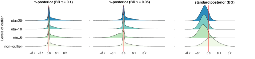
Figure 1: Oneshot example for the three posteriors of $\omega_{2,5}$ in the scenario (c-B) . From left to right, the posteriors are $\gamma$-posteriors under $\gamma=0.1,0.05$ (BR) and standard posterior (BG). From bottom to top, the levels of outliers are non-outlier, $\eta=5,10,20$ respectively.

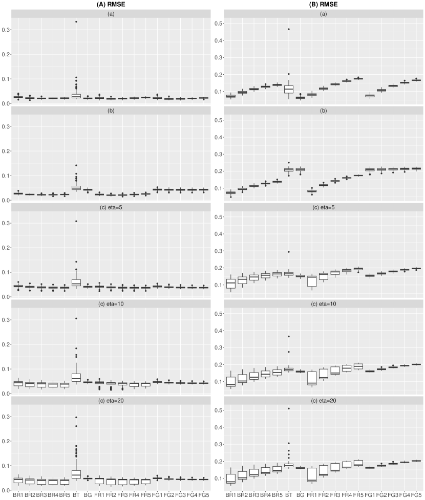
Figure 2: The boxplots of RMSE based on 100 repetitions for all scenarios are summarized. The left and right panels correspond to the results for (A) and (B), respectively, and the results for the five data-generating processes are summarized from top to bottom.

Table 1: The mean of AL and CP based on 100 repetitions for all scenarios are summarized.

Data-generating process (a)
		BR					BT	BG
		0.02	0.04	0.06	0.08	0.1
(A)	AL	0.107	0.098	0.092	0.087	0.083	0.180	0.087
	CP	0.931	0.910	0.891	0.872	0.847	0.971	0.966
(B)	AL	0.284	0.267	0.254	0.241	0.230	0.353	0.241
	CP	0.911	0.860	0.812	0.763	0.722	0.854	0.940
Data-generating process (b)
		BR					BT	BG
		0.02	0.04	0.06	0.08	0.1
(A)	AL	0.112	0.102	0.096	0.091	0.087	0.172	0.046
	CP	0.938	0.918	0.899	0.879	0.865	0.825	0.734
(B)	AL	0.299	0.280	0.265	0.251	0.239	0.193	0.078
	CP	0.917	0.869	0.827	0.783	0.742	0.507	0.473
Data-generating process (c) $\eta=5$
		BR					BT	BG
		0.02	0.04	0.06	0.08	0.1
(A)	AL	0.099	0.092	0.087	0.083	0.080	0.183	0.079
	CP	0.901	0.887	0.866	0.845	0.830	0.937	0.927
(B)	AL	0.288	0.266	0.250	0.235	0.223	0.284	0.193
	CP	0.896	0.837	0.788	0.738	0.691	0.779	0.773
Data-generating process (c) $\eta=10$
		BR					BT	BG
		0.02	0.04	0.06	0.08	0.1
(A)	AL	0.107	0.099	0.093	0.088	0.085	0.179	0.076
	CP	0.928	0.913	0.892	0.871	0.856	0.932	0.926
(B)	AL	0.292	0.271	0.255	0.241	0.229	0.274	0.189
	CP	0.906	0.852	0.807	0.760	0.712	0.768	0.772
Data-generating process (c) $\eta=20$
		BR					BT	BG
		0.02	0.04	0.06	0.08	0.1
(A)	AL	0.108	0.099	0.093	0.088	0.085	0.163	0.075
	CP	0.929	0.912	0.891	0.873	0.858	0.926	0.925
(B)	AL	0.293	0.272	0.256	0.242	0.230	0.247	0.188
	CP	0.908	0.857	0.810	0.765	0.719	0.752	0.771

Table 2: The mean of TPR and FPR based on 100 repetitions for all scenarios are summarized.

Data-generating process (a)
		BR1	BR2	BR3	BR4	BR5	FR1	FR2	FR3	FR4	FR5	FG1	FG2	FG3	FG4	FG5
(A)	TPR	0.11	0.54	0.71	0.80	0.86	0.20	0.36	0.49	0.59	0.67	0.17	0.32	0.45	0.54	0.61
	FPR	0.09	0.18	0.23	0.26	0.30	0.04	0.07	0.10	0.14	0.17	0.03	0.06	0.09	0.11	0.14
(B)	TPR	0.03	0.59	0.74	0.81	0.85	0.39	0.57	0.68	0.75	0.80	0.35	0.53	0.64	0.72	0.76
	FPR	0.00	0.00	0.02	0.05	0.09	0.00	0.01	0.03	0.08	0.14	0.00	0.00	0.02	0.05	0.09
Data-generating process (b)
		BR1	BR2	BR3	BR4	BR5	FR1	FR2	FR3	FR4	FR5	FG1	FG2	FG3	FG4	FG5
(A)	TPR	0.08	0.48	0.68	0.78	0.84	0.20	0.35	0.47	0.58	0.66	0.05	0.10	0.15	0.19	0.24
	FPR	0.08	0.16	0.22	0.27	0.31	0.04	0.07	0.10	0.13	0.18	0.03	0.05	0.08	0.10	0.13
(B)	TPR	0.01	0.56	0.72	0.80	0.85	0.37	0.56	0.67	0.75	0.80	0.06	0.13	0.18	0.23	0.28
	FPR	0.00	0.01	0.02	0.06	0.10	0.00	0.01	0.03	0.08	0.15	0.04	0.09	0.13	0.17	0.21
Data-generating process (c) $\eta=5$
		BR1	BR2	BR3	BR4	BR5	FR1	FR2	FR3	FR4	FR5	FG1	FG2	FG3	FG4	FG5
(A)	TPR	0.11	0.51	0.69	0.78	0.83	0.17	0.31	0.44	0.54	0.62	0.14	0.28	0.39	0.48	0.57
	FPR	0.08	0.18	0.22	0.26	0.29	0.04	0.08	0.11	0.14	0.16	0.04	0.07	0.09	0.12	0.14
(B)	TPR	0.01	0.55	0.72	0.79	0.84	0.34	0.53	0.64	0.73	0.79	0.28	0.45	0.58	0.66	0.73
	FPR	0.00	0.01	0.04	0.08	0.12	0.01	0.03	0.07	0.11	0.18	0.01	0.02	0.05	0.08	0.14
Data-generating process (c) $\eta=10$
		BR1	BR2	BR3	BR4	BR5	FR1	FR2	FR3	FR4	FR5	FG1	FG2	FG3	FG4	FG5
(A)	TPR	0.10	0.50	0.69	0.78	0.84	0.17	0.31	0.43	0.53	0.60	0.13	0.26	0.37	0.46	0.54
	FPR	0.08	0.18	0.22	0.26	0.29	0.04	0.08	0.11	0.13	0.16	0.04	0.08	0.09	0.12	0.14
(B)	TPR	0.01	0.56	0.72	0.80	0.84	0.35	0.53	0.63	0.72	0.77	0.27	0.43	0.55	0.63	0.69
	FPR	0.00	0.01	0.03	0.07	0.12	0.01	0.02	0.05	0.10	0.16	0.01	0.03	0.05	0.08	0.14
Data-generating process (c) $\eta=20$
		BR1	BR2	BR3	BR4	BR5	FR1	FR2	FR3	FR4	FR5	FG1	FG2	FG3	FG4	FG5
(A)	TPR	0.10	0.50	0.69	0.79	0.85	0.17	0.31	0.43	0.52	0.59	0.13	0.25	0.36	0.44	0.52
	FPR	0.08	0.18	0.22	0.26	0.29	0.04	0.08	0.11	0.13	0.16	0.03	0.08	0.09	0.12	0.13
(B)	TPR	0.01	0.56	0.72	0.80	0.85	0.35	0.52	0.63	0.71	0.76	0.27	0.43	0.54	0.61	0.66
	FPR	0.00	0.01	0.03	0.07	0.11	0.00	0.02	0.05	0.10	0.16	0.01	0.03	0.05	0.08	0.14

Real data example

We apply the proposed method to the yeast gene expression data (Gasch et al., 2000). Following Hirose et al. (2017), we focused on analyzing $p=8$ genes involved in galactose utilization (Ideker et al., 2001). The sample size is $n=136$. Conducting a principal component analysis, we can see 11 outliers in this dataset (see also Finegold and Drton, 2011; Hirose et al., 2017). Hirose et al. (2017) mentioned that there are two additional outliers, and they consider 13 outliers. Following their study, we compared the two datasets with/without outliers, and the data were normalized with median and median absolute deviation (MAD).

We here deal with the data removed the 13 outliers as a clean dataset (the sample size is $123$), and regard the corresponding estimates as the true estimates for convenience. We compared the proposed method with two frequentist methods presented in Section 4. The tuning parameter $\lambda$ was selected so that the number of edges is 9 as in Hirose et al. (2017). Note that the BR method determines whether zero or not via posterior probability in Section 2.5 and 6000 posterior samples were drawn by the WBB algorithm. The applied results are reported in Figures 3 and 4. From Figure 3, there are no differences between the left (without outliers) and right (with outliers) panels for the solution paths based on the BR and FR methods while the FR method is affected by outliers because of non-robustness. Comparing the BR method and the FR method, only one edge is differently estimated. However, the result is not strange because the variable selection method for the two methods is different. Indeed, the scatter plot in the left panel of Figure 4, which represents the posterior probabilities of zero estimate for BR methods and the relationships between the BR and FR methods, shows that the colors indicating whether the estimates based on the FR method are zero or not cross near 50% posterior probability. The posterior probabilities for the data included outliers are similar to that of the data without outliers because the scatter plot is close to the straight line ($y=x$). The 95% credible intervals (CI) for the BR methods are also shown in the right panel in Figure 4. The CIs for non-zero estimates based on posterior probability correspond to dark-colored vars. It is considered that the posterior means and CIs for these vars are relatively far from zero. From the posterior probabilities and the credible intervals in Figure 4, it seems that the posterior robustness holds, and the BR method gives the uncertainty for shrinkage via posterior probability and credible intervals.

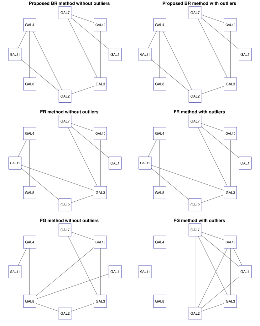
Figure 3: The solution path via BR, FR, and FG from top to bottom. The right panels are based on the data without 13 outliers, and the left panels are based on all data with outliers.

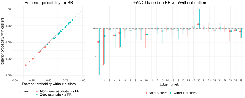
Figure 4: The comparison of posterior probability and 95% credible intervals based on the data with/without outliers. In the right panels, the dark-colored vars are non-zero elements based on posterior probability, and the corresponding edges are drawn in Figure 3.

Concluding remarks

A robust Bayesian graphical lasso based on the $\gamma$-divergence was proposed. The proposed posterior distribution was constructed by matching the MAP estimate with the frequentist estimate by Hirose et al. (2017). It was shown that the proposed model has a desirable robustness property called posterior robustness. There are some future works as follows. First, although we focused on using the Laplace prior in this paper, the proposed method can be extended to other types of shrinkage priors. Since the proposed MAP $\gamma$-posterior under popular spike-and-slab (e.g. Wang, 2015) and horseshoe (e.g. Li et al., 2019) priors is proper by carefully selecting priors for the diagonal elements (Theorem 1), the posterior robustness still holds. However, the approximation of posterior distribution is not straightforward. Second, in the proposed optimization-based sampling algorithm based on the WBB, the random weight vector distributed as the Dirichlet distribution (see Subsection 2.4) is interpretable as the parameter that controls the spread of the posterior distribution. Hence, by calibrating the hyper-parameters in the Dirichlet distribution, we may derive valid credible intervals in the presence of outliers.

Supplementary Materials for “Robust Bayesian graphical modeling using $\gamma$-divergence”

Takahiro Onizuka and Shintaro Hashimoto

Department of Mathematics, Hiroshima University, Japan

We provide the proofs of Propositions 1, 2, and 3, details of algorithms, and additional information for the simulation study.

Proofs of propositions

In this section, we give the proofs for three propositions.

Proof of Proposition 1

Proof.

The ratio of the posterior densities is expressed by

$$\frac{\pi(\Omega\mid D)}{\pi(\Omega\mid D^{*})} =\frac{p(D^{*})}{p(D)}\frac{\prod_{i=1}^{n}|\Omega|^{1/2}\exp\left(-y_{i}^{\top}\Omega y_{i}/2\right)}{\prod_{i\in\mathcal{K}}|\Omega|^{1/2}\exp\left(-y_{i}^{\top}\Omega y_{i}/2\right)}$$

$$=\frac{p(D^{*})}{p(D)}\prod_{i\in\mathcal{L}}|\Omega|^{1/2}\exp\left(-y_{i}^{\top}\Omega y_{i}/2\right),$$

where

$$p(D) =\int\prod_{i=1}^{n}|\Omega|^{1/2}\exp\left(-y_{i}^{\top}\Omega y_{i}/2\right)\pi(\Omega)d\Omega,$$

$$p(D^{*}) =\int\prod_{i\in\mathcal{K}}|\Omega|^{1/2}\exp\left(-y_{i}^{\top}\Omega y_{i}/2\right)\pi(\Omega)d\Omega.$$

Since $y_{i}\neq 0$ for $i\in\mathcal{L}$, we obtain

$$p(D) =\int\prod_{i=1}^{n}|\Omega|^{1/2}\exp\left(-y_{i}^{\top}\Omega y_{i}/2\right)\pi(\Omega)d\Omega$$

$$=\int\prod_{i\in\mathcal{L}}|\Omega|^{1/2}\exp\left(-y_{i}^{\top}\Omega y_{i}/2\right)\prod_{i\in\mathcal{K}}|\Omega|^{1/2}\exp\left(-y_{i}^{\top}\Omega y_{i}/2\right)\pi(\Omega)d\Omega$$

$$\leq C\int\prod_{i\in\mathcal{K}}|\Omega|^{1/2}\exp\left(-y_{i}^{\top}\Omega y_{i}/2\right)\pi(\Omega)d\Omega=Cp(D^{*}),$$

where $C$ is a constant. Hence, we have

$$\frac{\pi(\Omega\mid D)}{\pi(\Omega\mid D^{*})} =\frac{p(D^{*})}{p(D)}\prod_{i\in\mathcal{L}}|\Omega|^{1/2}\exp\left(-y_{i}^{\top}\Omega y_{i}/2\right)$$

$$\geq\frac{p(D^{*})}{Cp(D^{*})}\prod_{i\in\mathcal{L}}|\Omega|^{1/2}\exp\left(-y_{i}^{\top}\Omega y_{i}/2\right)$$

$$=\frac{1}{C}\prod_{i\in\mathcal{L}}|\Omega|^{1/2}\exp\left(-y_{i}^{\top}\Omega y_{i}/2\right)$$

and

$$\lim_{z\to\infty}\frac{\pi(\Omega\mid D)}{\pi(\Omega\mid D^{*})} =\lim_{z\to\infty}\frac{1}{C}\prod_{i\in\mathcal{L}}|\Omega|^{1/2}\exp\left(-y_{i}^{\top}\Omega y_{i}/2\right)=0.$$

Using the same argument as Theorem 2, we have

$$\lim_{z\to\infty}\int|\pi(\Omega\mid D)-\pi(\Omega\mid D^{*})|d\Omega=1\neq 0.$$

This completes the proof. ∎

Proof of Proposition 2

Proof.

The ratio of the posterior densities is expressed by

$$\frac{\pi(\Omega\mid D)}{\pi(\Omega\mid D^{*})} =\frac{p(D^{*})}{p(D)}\frac{\prod_{i=1}^{n}|\Omega|^{1/2}\left[1+y_{i}^{\top}\Omega y_{i}/(\nu-2)\right]^{-(\nu+p)}}{\prod_{i\in\mathcal{K}}|\Omega|^{1/2}\left[1+y_{i}^{\top}\Omega y_{i}/(\nu-2)\right]^{-(\nu+p)}}$$

$$=\frac{p(D^{*})}{p(D)}\prod_{i\in\mathcal{L}}|\Omega|^{1/2}\left[1+y_{i}^{\top}\Omega y_{i}/(\nu-2)\right]^{-(\nu+p)},$$

where

$$p(D) =\int\prod_{i=1}^{n}|\Omega|^{1/2}\left[1+y_{i}^{\top}\Omega y_{i}/(\nu-2)\right]^{-(\nu+p)}\pi(\Omega)d\Omega$$

$$p(D^{*}) =\int\prod_{i\in\mathcal{K}}|\Omega|^{1/2}\left[1+y_{i}^{\top}\Omega y_{i}/(\nu-2)\right]^{-(\nu+p)}\pi(\Omega)d\Omega.$$

Since $y_{i}\neq 0$ for $i\in\mathcal{L}$, we obtain

$$p(D) =\int\prod_{i=1}^{n}|\Omega|^{1/2}\left[1+y_{i}^{\top}\Omega y_{i}/(\nu-2)\right]^{-(\nu+p)}\pi(\Omega)d\Omega$$

$$=\int\prod_{i\in\mathcal{L}}|\Omega|^{1/2}\left[1+y_{i}^{\top}\Omega y_{i}/(\nu-2)\right]^{-(\nu+p)}\prod_{i\in\mathcal{K}}|\Omega|^{1/2}\left[1+y_{i}^{\top}\Omega y_{i}/(\nu-2)\right]^{-(\nu+p)}\pi(\Omega)d\Omega$$

$$\leq C\int\prod_{i\in\mathcal{K}}|\Omega|^{1/2}\left[1+y_{i}^{\top}\Omega y_{i}/(\nu-2)\right]^{-(\nu+p)}\pi(\Omega)d\Omega=Cp(D^{*}),$$

where $C$ is a constant. Then we have

$$\frac{\pi(\Omega\mid D)}{\pi(\Omega\mid D^{*})} =\frac{p(D^{*})}{p(D)}\prod_{i\in\mathcal{L}}|\Omega|^{1/2}\left[1+y_{i}^{\top}\Omega y_{i}/(\nu-2)\right]^{-(\nu+p)}$$

$$\geq\frac{p(D^{*})}{Cp(D^{*})}\prod_{i\in\mathcal{L}}|\Omega|^{1/2}\left[1+y_{i}^{\top}\Omega y_{i}/(\nu-2)\right]^{-(\nu+p)}$$

$$=\frac{1}{C}\prod_{i\in\mathcal{L}}|\Omega|^{1/2}\left[1+y_{i}^{\top}\Omega y_{i}/(\nu-2)\right]^{-(\nu+p)}$$

and

$$\lim_{z\to\infty}\frac{\pi(\Omega\mid D)}{\pi(\Omega\mid D^{*})} =\lim_{z\to\infty}\frac{1}{C}\prod_{i\in\mathcal{L}}|\Omega|^{1/2}\left[1+y_{i}^{\top}\Omega y_{i}/(\nu-2)\right]^{-(\nu+p)}=0.$$

Using the same argument as Theorem 2, we have

$$\lim_{z\to\infty}\int|\pi(\Omega\mid D)-\pi(\Omega\mid D^{*})|d\Omega=1\neq 0.$$

This completes the proof. ∎

Proof of Proposition 3

Proof.

The ratio of the posterior densities is expressed by

$$\frac{\pi_{\mathrm{DP}}(\Omega\mid D)}{\pi_{\mathrm{DP}}(\Omega\mid D^{*})} =\frac{p(D^{*})}{p(D)}\frac{\exp\left(Q_{n}^{(\alpha)}(D\mid\Omega)\right)}{\exp\left(Q_{n}^{(\alpha)}(D^{*}\mid\Omega)\right)},$$

where

$$Q_{n}^{(\alpha)}(D\mid\Omega) =(2\pi)^{-\alpha p/2}|\Omega|^{\alpha/2}\left[\frac{1}{\alpha}\sum_{i=1}^{n}\exp\left(-\frac{\alpha}{2}y_{i}^{\top}\Omega y_{i}\right)-n(1+\alpha)^{1-\alpha/2}\right],$$

$$Q_{n}^{(\alpha)}(D^{*}\mid\Omega) =(2\pi)^{-\alpha p/2}|\Omega|^{\alpha/2}\left[\frac{1}{\alpha}\sum_{i\in\mathcal{K}}\exp\left(-\frac{\alpha}{2}y_{i}^{\top}\Omega y_{i}\right)-|\mathcal{K}|(1+\alpha)^{1-\alpha/2}\right],$$

$$p(D) =\int\exp\left(Q_{n}^{(\alpha)}(D\mid\Omega)\right)\pi(\Omega)d\Omega,$$

$$p(D^{*}) =\int\exp\left(Q_{n}^{(\alpha)}(D^{*}\mid\Omega)\right)\pi(\Omega)d\Omega.$$

Then we obtain

$$\lim_{z\to\infty}\exp\left(Q_{n}^{(\alpha)}(D\mid\Omega)\right)$$

$$=\lim_{z\to\infty}\exp\left[(2\pi)^{-\alpha p/2}|\Omega|^{\alpha/2}\left\{\frac{1}{\alpha}\sum_{i=1}^{n}\exp\left(-\frac{\alpha}{2}y_{i}^{\top}\Omega y_{i}\right)-n(1+\alpha)^{1-\alpha/2}\right\}\right]$$

$$=\exp\left[(2\pi)^{-\alpha p/2}|\Omega|^{\alpha/2}\left\{\frac{1}{\alpha}\sum_{i\in\mathcal{K}}\exp\left(-\frac{\alpha}{2}y_{i}^{\top}\Omega y_{i}\right)-n(1+\alpha)^{1-\alpha/2}\right\}\right]$$

$$=\exp\left[(2\pi)^{-\alpha p/2}|\Omega|^{\alpha/2}\frac{1}{\alpha}\sum_{i\in\mathcal{K}}\exp\left(-\frac{\alpha}{2}y_{i}^{\top}\Omega y_{i}\right)\right]\exp\left[-(2\pi)^{-\alpha p/2}n(1+\alpha)^{1-\alpha/2}|\Omega|^{\alpha/2}\right]$$

$$=\exp\left(Q_{n}^{(\alpha)}(D^{*}\mid\Omega)\right)\exp\left[-(2\pi)^{-\alpha p/2}(n-|\mathcal{K}|)(1+\alpha)^{1-\alpha/2}|\Omega|^{\alpha/2}\right].$$

From Lebesgue’s dominated convergence theorem, it holds that

$$\lim_{z\to\infty}p(D) =\lim_{z\to\infty}\int\exp\left(Q_{n}^{(\alpha)}(D\mid\Omega)\right)\pi(\Omega)d\Omega$$

$$=\int\lim_{z\to\infty}\exp\left(Q_{n}^{(\alpha)}(D\mid\Omega)\right)\pi(\Omega)d\Omega$$

$$=\int\exp\left(Q_{n}^{(\alpha)}(D^{*}\mid\Omega)\right)\exp\left[-(2\pi)^{-\alpha p/2}(n-|\mathcal{K}|)(1+\alpha)^{1-\alpha/2}|\Omega|^{\alpha/2}\right]\pi(\Omega)d\Omega$$

$$=C_{D^{*}}>0,$$

where $C_{D^{*}}$ is a constant that does not depend on $\Omega$, and we have $\lim_{z\to\infty}p(D^{*})/p(D)=p(D^{*})/C_{D^{*}}$. Therefore, the limit of the ratio is calculated by

$$\lim_{z\to\infty}\frac{\pi(\Omega\mid D)}{\pi(\Omega\mid D^{*})} =\frac{p(D^{*})}{C_{D^{*}}}\exp\left[-(2\pi)^{-\alpha p/2}(n-|\mathcal{K}|)(1+\alpha)^{1-\alpha/2}|\Omega|^{\alpha/2}\right]\neq 1.$$

This completes the proof. ∎

The details of algorithms

We summarized the details of two algorithms: weighted Bayesian bootstrap via MM algorithm, and Gibbs sampler for t-likelihood.

Derivation of $L_{w}^{*}(\Omega)$ in (9)

Considering the lasso type prior

$$\pi(\Omega) \propto\exp(-\lambda\|\Omega\|_{1})1_{\{\Omega\in M^{+}\}}=\prod_{i\leq j}\mathrm{Lap}(w_{ij}\mid\lambda)1_{\{\Omega\in M^{+}\}}$$

$$=\prod_{i=1}^{p}\mathrm{Exp}(w_{ii}\mid\lambda)\prod_{i<j}^{p}\mathrm{Lap}(w_{ij}\mid\lambda)1_{\{\Omega\in M^{+}\}},$$

the weighted objective function is given by

$$L_{w}(\Omega) =-\frac{1}{\gamma}\log\left[\frac{1}{n}\sum_{i=1}^{n}w_{i}\frac{f(y_{i}\mid\Omega)^{\gamma}}{\int f(y\mid\Omega)^{1+\gamma}dy}\right]+\lambda w_{0}\|\Omega\|_{1}$$

$$=-\frac{1}{\gamma}\log\left\{\frac{1}{n}\sum_{i=1}^{n}w_{i}f(y_{i}\mid\Omega)^{\gamma}\right\}+\frac{\gamma}{2(1+\gamma)}\log|\Omega|+\lambda w_{0}\|\Omega\|_{1},$$

where $(w_{0},w_{1},\dots,w_{n})$ is a weight. By using Jensen’s inequality, the first term is bounded by

$$-\frac{1}{\gamma}\log\left\{\frac{1}{n}\sum_{i=1}^{n}w_{i}f(y_{i}\mid\Omega)^{\gamma}\right\}\leq C_{1}-\frac{1}{2}\log|\Omega|+\frac{1}{2}\sum_{i=1}^{n}s_{i}^{*}y_{i}^{\top}\Omega y_{i},$$

where $s_{i}^{*}=w_{i}f(y_{i}\mid\Omega)^{\gamma}/\sum_{j=1}^{n}w_{j}f(y_{j}\mid\Omega)^{\gamma}$ and $C_{1}$ is a constant. Therefore, the objective function $L_{w}(\Omega)$ is bounded by

$$L_{w}(\Omega) =-\frac{1}{\gamma}\log\left\{\sum_{i=1}^{n}w_{i}f(y_{i}\mid\Omega)^{\gamma}\right\}+\frac{\gamma}{2(1+\gamma)}\log|\Omega|+\lambda w_{0}\|\Omega\|_{1}$$

$$\leq\frac{1}{2(1+\gamma)}\left[\mathrm{tr}\left\{\left((1+\gamma)\sum_{i=1}^{n}s_{i}^{*}y_{i}y_{i}^{\top}\right)\Omega\right\}-\log|\Omega|+2(1+\gamma)\lambda w_{0}\|\Omega\|_{1}\right]$$

$$\propto\mathrm{tr}\left\{S^{*}\Omega\right\}-\log|\Omega|+\rho\|\Omega\|_{1},$$

where

$$S^{*} =(1+\gamma)\sum_{i=1}^{n}s_{i}^{*}y_{i}y_{i}^{\top},\quad\rho=2(1+\gamma)\lambda w_{0}.$$

MCMC algorithm for Bayesian $t$-graphical lasso

The joint probability density function of the multivariate $t$-distribution is given by

$$p(y\mid\Sigma)\propto\prod_{i=1}^{n}p(y_{i}\mid\Sigma)\propto\prod_{i=1}^{n}|\Sigma|^{-1/2}\left(1+\frac{1}{\nu}y_{i}^{\top}\Sigma^{-1}y_{i}\right),$$

where $\nu$ is the degrees of freedom and the covariance matrix is $\{\nu/(\nu-2)\}\Sigma$ for $\nu>2$. By using the Gaussian scale mixture representation of t-distribution, the conditional density is given by

$$y_{i}\mid\Sigma,u\sim N_{p}(0,\Sigma/u),\quad u\sim\mathrm{Ga}(\nu/2,\nu/2)$$

We define the precision matrix $\Omega=(\{\nu/(\nu-2)\}\Sigma)^{-1}$, and then the densities are rewritten as

$$p(y\mid\Omega,u) \propto u^{np/2}|\Omega|^{n/2}\exp\left(-\frac{\nu u}{2(\nu-2)}\sum_{i=1}^{n}y_{i}^{\top}\Omega y_{i}\right)$$

$$p(u) \propto u^{-1+\nu/2}\exp\left(-\frac{\nu}{2}u\right)$$

For the prior of $\Omega$, we assume Laplace and exponential prior:

$$p(\Omega\mid\tau,\lambda) \propto\prod_{i<j}\left[\tau_{ij}^{-1/2}\exp\left(-\frac{\omega_{ij}^{2}}{2\tau_{ij}}\right)\right]\prod_{i=1}^{p}\left[\exp\left(-\frac{\lambda}{2}\omega_{ij}\right)\right]1_{\Omega\in M^{+}},$$

$$p(\tau\mid\lambda) \propto\prod_{i<j}\left[\exp\left(-\frac{\lambda^{2}}{2}\tau_{ij}\right)\right].$$

From this formulation, we can construct a Gibbs sampler based on block Gibbs sampler (Wang, 2012). The full conditional distribution of $u$ is given by

$$p(u\mid y,\Omega)\sim\mathrm{Ga}\left(\frac{np+\nu}{2},\frac{\nu}{2(\nu-2)}\sum_{i=1}^{n}y_{i}^{\top}\Omega y_{i}+\frac{\nu}{2}\right).$$

Additional simulation information

True precision matrix

The true precision matrix (A) in the simulation study is as follows:

$$\left(\begin{array}[]{cccccccccccc}0.239&0.117&&&&&&0.031&&&&\\ 0.117&1.554&&&&&&&&&&\\ &&0.362&0.002&&&&&&&&\\ &&0.002&0.199&0.094&&&&&&&\\ &&&0.094&0.349&&&&&&&-0.036\\ &&&&&0.295&-0.229&0.002&&&&\\ &&&&&-0.229&0.715&&&&&\\ 0.031&&&&&0.002&&0.164&0.112&-0.028&-0.008&\\ &&&&&&&0.112&0.518&-0.193&-0.09&\\ &&&&&&&-0.028&-0.193&0.379&0.167&\\ &&&&&&&-0.008&-0.09&0.167&0.159&\\ &&&&-0.036&&&&&&&0.207\\ \end{array}\right)$$

Simulation results

We reported the simulation results for the BR and FR methods for $\gamma=0.05$. To compare with the $\gamma=0.1$, we showed the results for $\gamma=0.1$ which is also reported in the main manuscript. The results are summarized in Figure S1. For scenario (a), which does not include outliers, the results for $\gamma=0.05$ are similar to that for $\gamma=0.1$. However, the $\gamma=0.1$ holds more robustness for the scenario in which the outliers are heavy.

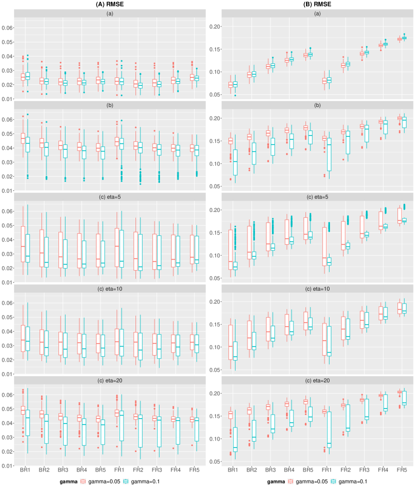
Figure S1: The boxplots of RMSE based on 100 repetitions for all scenarios are summarized. The left and right panels correspond to the results for (A) and (B), respectively, and the results for the five data-generating processes are summarized from top to bottom.

References

- Barbieri and Berger (2004) Barbieri, M. M. and J. O. Berger (2004). Optimal predictive model selection. The Annals of Statistics 32(3), 870 – 897.
- Basu et al. (1998) Basu, A., I. R. Harris, N. L. Hjort, and M. Jones (1998). Robust and efficient estimation by minimising a density power divergence. Biometrika 85(3), 549–559.
- Berger et al. (2009) Berger, J. O., J. M. Bernardo, and D. Sun (2009). The formal definition of reference priors. The Annals of Statistics 37(2), 905–938.
- Desgagné (2015) Desgagné, A. (2015). Robustness to outliers in location–scale parameter model using log-regularly varying distributions. The Annals of Statistics 43(4), 1568–1595.
- Desgagné and Gagnon (2019) Desgagné, A. and P. Gagnon (2019). Bayesian robustness to outliers in linear regression and ratio estimation. Brazilian Journal of Probability and Statistics 32(2), 205–221.
- Fan et al. (2009) Fan, J., Y. Feng, and Y. Wu (2009). Network exploration via the adaptive lasso and scad penalties. The Annals of Applied Statistics 3(2), 521.
- Finegold and Drton (2011) Finegold, M. and M. Drton (2011). Robust graphical modeling of gene networks using classical and alternative t-distributions. 5(2), 1057–1080.
- Friedman et al. (2008) Friedman, J., T. Hastie, and R. Tibshirani (2008). Sparse inverse covariance estimation with the graphical lasso. Biostatistics 9(3), 432–441.
- Fujisawa and Eguchi (2008) Fujisawa, H. and S. Eguchi (2008). Robust parameter estimation with a small bias against heavy contamination. Journal of Multivariate Analysis 99(9), 2053–2081.
- Gagnon et al. (2020) Gagnon, P., A. Desgagné, and M. Bédard (2020). A new bayesian approach to robustness against outliers in linear regression. Bayesian Analysis 15(2), 389–414.
- Gasch et al. (2000) Gasch, A. P., P. T. Spellman, C. M. Kao, O. Carmel-Harel, M. B. Eisen, G. Storz, D. Botstein, and P. O. Brown (2000). Genomic expression programs in the response of yeast cells to environmental changes. Molecular biology of the cell 11(12), 4241–4257.
- Ghosh and Basu (2016) Ghosh, A. and A. Basu (2016). Robust bayes estimation using the density power divergence. Annals of the Institute of Statistical Mathematics 68, 413–437.
- Hamura et al. (2022) Hamura, Y., K. Irie, and S. Sugasawa (2022). Log-regularly varying scale mixture of normals for robust regression. Computational Statistics & Data Analysis 173, 107517.
- Hashimoto and Sugasawa (2020) Hashimoto, S. and S. Sugasawa (2020). Robust bayesian regression with synthetic posterior distributions. Entropy 22(6), 661.
- Hirose et al. (2017) Hirose, K., H. Fujisawa, and J. Sese (2017). Robust sparse gaussian graphical modeling. Journal of Multivariate Analysis 161, 172–190.
- Ideker et al. (2001) Ideker, T., V. Thorsson, J. A. Ranish, R. Christmas, J. Buhler, J. K. Eng, R. Bumgarner, D. R. Goodlett, R. Aebersold, and L. Hood (2001). Integrated genomic and proteomic analyses of a systematically perturbed metabolic network. Science 292(5518), 929–934.
- Lauritzen (1996) Lauritzen, S. L. (1996). Graphical models, Volume 17. Clarendon Press.
- Li et al. (2019) Li, Y., B. A. Craig, and A. Bhadra (2019). The graphical horseshoe estimator for inverse covariance matrices. Journal of Computational and Graphical Statistics 28(3), 747–757.
- Lyddon et al. (2019) Lyddon, S. P., C. Holmes, and S. Walker (2019). General bayesian updating and the loss-likelihood bootstrap. Biometrika 106(2), 465–478.
- Maronna et al. (2019) Maronna, R. A., R. D. Martin, V. J. Yohai, and M. Salibián-Barrera (2019). Robust Statistics: Theory and Methods (with R). John Wiley & Sons.
- Momozaki and Nakagawa (2023) Momozaki, T. and T. Nakagawa (2023). Robustness of bayesian ordinal response model against outliers via divergence approach. arXiv preprint arXiv:2305.07553.
- Nakagawa and Hashimoto (2020) Nakagawa, T. and S. Hashimoto (2020). Robust bayesian inference via -divergence. Communications in Statistics-Theory and Methods 49(2), 343–360.
- Newton et al. (2021) Newton, M. A., N. G. Polson, and J. Xu (2021). Weighted bayesian bootstrap for scalable posterior distributions. Canadian Journal of Statistics 49(2), 421–437.
- Nie and Ročková (2022) Nie, L. and V. Ročková (2022). Bayesian bootstrap spike-and-slab lasso. Journal of the American Statistical Association, 1–16.
- Park and Casella (2008) Park, T. and G. Casella (2008). The bayesian lasso. Journal of the American Statistical Association 103(482), 681–686.
- Sun and Li (2012) Sun, H. and H. Li (2012). Robust gaussian graphical modeling via l1 penalization. Biometrics 68(4), 1197–1206.
- Wang (2012) Wang, H. (2012). Bayesian graphical lasso models and efficient posterior computation. Bayesian Analysis 7(4), 867–886.
- Wang (2015) Wang, H. (2015). Scaling it up: Stochastic search structure learning in graphical models. Bayesian Analysis 10(2), 351–377.
- Whittaker (2009) Whittaker, J. (2009). Graphical models in applied multivariate statistics. Wiley Publishing.
- Yonekura and Sugasawa (2023) Yonekura, S. and S. Sugasawa (2023). Adaptation of the tuning parameter in general bayesian inference with robust divergence. Statistics and Computing 33(2), 39.
- Yuan and Lin (2007) Yuan, M. and Y. Lin (2007). Model selection and estimation in the gaussian graphical model. Biometrika 94(1), 19–35.