Spontaneous charge current in time-reversal-symmetry breaking phase in kagome metals

Abstract

The charge loop current (cLC) state has attracted increasing attention in kagome metals. Here, we calculate the spontaneous currents along the nearest sites $i$ and $j$, $J_{i,j}$, induced by the cLC order that is the imaginary and odd-parity hopping integral modulation $\delta t_{i,j}$. We reveal that the magnitude of $J_{i,j}$ strongly depends on the nearest sites $i$ and $j$ in the $2\times 2$ cLC state, where $\eta\equiv|\delta t_{i,j}|$ is equivalent for all nearest sites. The obtained $J_{i,j}$ becomes large near the van-Hove singularity (vHS) filling ($n\sim n_{\rm vHS}$) even when $\eta$ is fixed. Interestingly, the obtained $J_{i,j}$ exhibits the logarithmic divergence behavior at low temperatures for $n\sim n_{\rm vHS}$ with a fixed $\eta$, by reflecting the vHS points that are the characteristic of kagome metals. The present study provides useful information for local electronic state measurements, such as the site-selective NMR and STM experiments.

Introduction - In recent years, kagome lattice metals have become one of central topics in the field of strongly correlated electron systems. Multiple exotic metallic phase transitions, such as the star-of-David bond-order (BO), superconducting (SC) state, and time-reversal-symmetry-breaking (TRSB) phase without spin polarization, are realized thanks to the strong geometrical frustration that prevents simple spin and charge orders. In $A$V₃Sb₅ ($A$=Cs,Rb,K), the $2\times 2$ BO appears at $T_{\rm BO}\approx 100$K [1, 2]. Inside the BO phase, the SC state appears at $T_{\rm SC}\approx 1-10$K [3, 4, 5, 6, 7]. In addition, the electronic nematic state has been observed inside [8, 9, 10] and outside [11] of the BO phase. To explain the observed nematicity, the single-${\bm{Q}}$ odd-parity BO [12] and $E_{g}$ symmetry nematic BO [13] have been proposed theoretically.

To understand these exotic electronic states in kagome metals, various theoretical studies have been performed, based on the extended mean-field theory [14, 15], the functional renormalization group (RG) theory [16, 17], the parquet RG theory [19, 18], and the density-wave (DW) equation analysis with the higher-order vertex corrections (VCs) [20]. Both the RG theory and the DW equation theory have been successfully applied to Fe-based [21, 22, 23, 38, 39, 43] and cuprate superconductors [44]. The nematic order and the BO in these systems originate from the higher-order VCs [38]. Recently, the present authors proposed a unified explanation for the BO and the heavily anisotropic $s$ wave SC state in kagome metals based on the DW equation analysis [20]. However, theoretical understanding for the TRSB state has been limited until recently.

Recently, the TRSB state has been observed by various experimental methods. Inside the BO phase, the TRSB has been observed by the STM [1], the $\mu$SR [27, 28, 26], the anomalous Hall effect [24, 25], and the magnetochiral anisotropy (eMChA) [45, 29] measurements. The spontaneous charge loop-current (cLC) order is a natural candidate of the TRSB order. In kagome metals, the $2\times 2$ cLC order has finite orbital magnetization $M_{\rm orb}$; see Ref. [12]. References [45, 29] report that the TRSB domains with random chiralities are detwinned by the magnetic field $h_{z}\sim 1{\rm T}$, and $T_{\rm TRSB}$ is drastically enhanced by small $h_{z}$ as well as the uniaxial pressure ${\epsilon}$. Such drastic $h_{z}$- and ${\epsilon}$-dependences of the TRSB states are naturally explained based on the Ginzburg-Landau (GL) theory under $(h_{z},{\epsilon})$ in Ref. [12], owing to the finite $M_{\rm orb}$. Very interestingly, the TRSB state outside the BO phase ($T_{\rm TRSB}\approx 130$K) has been discovered by the recent magnetic torque measurement [11]. The single ${\bm{Q}}$ cLC order ($M_{\rm orb}=0$) is a natural candidate. Actually, the cLC order can emerge above $T_{\rm BO}$ theoretically [35].

The cLC order was originally studied in cuprate superconductors [31, 32, 33]. The cLC order is defined as the imaginary and odd-parity hopping integral modulation between sites $i$ and $j$, $\delta t_{i,j}$ [20, 35, 36]. The Berry curvature due to $\delta t_{i,j}$ gives rise to the spontaneous current [30]. To understand the microscopic origin of the cLC order in kagome metals, various theoretical studies have been performed, such as the mean-field theory [14, 15], the parquet RG theory [19, 18], and the DW equation analysis [35]. Importantly, the BO fluctuations in kagome metals mediate not only the SC pairing, but also the cLC order that is the TRSB particle-hole pair condensation; see Ref. [35]. Therefore, the cLC state is naturally expected to occur in kagome metals with the BO instability. Recently, the competition between the BO, cLC and the SC states is intensively studied based on the GL theories [19, 12, 40, 47].

In the cLC state in kagome metal model, the uniform orbital magnetization $M_{\rm orb}$ was recently studied in Ref. [12]. However, the nanoscale charge current flowing between the nearest bonds, $J_{i,j}$, has not been performed to our knowledge. The knowledge of $J_{i,j}$ is significant to understand the local magnetization measurements, such as the $\mu$SR [27, 28, 26] and the NMR [46] measurements.

In this Letter, we analyze the spontaneous current $J_{i,j}$ in the $2\times 2$ cLC order phase. We reveal that the magnitude of $J_{i,j}$ strongly depends on the nearest sites $(i,j)$. The obtained $J_{i,j}$ becomes large near the van-Hove singularity (vHS) filling ($n\sim n_{\rm vHS}$). Interestingly, $J_{i,j}$ exhibits the logarithmic divergence behavior at low temperatures for $n\sim n_{\rm vHS}$, by reflecting the vHS points that are the characteristic of kagome metals. The present study provides useful information for local electronic state measurements, such as the site-selective NMR and STM experiments.

Model Hamiltonian with $3\bm{Q}$ cLC order - First, we show a 3-site kagome lattice model in Fig. 1 (a). Here, the nearest-neighbor hopping integral is $t=-0.5$[eV]. Additionally, to prevent perfect nesting, a next-nearest-neighbor hopping integral is introduced with $t^{\prime}=-0.02$[eV]. There are three sites, A, B, and C in the unit cell. The vectors between nearest-neighboring sites are defined as $\bm{a}_{AB},\bm{a}_{BC}$, and $\bm{a}_{CA}$. Fig. 1 (b) shows the Fermi surface (FS) of the 3-site kagome lattice model and nesting vectors ${{\bm{q}}}_{n}$ $(n=1,2,3)$. There exist three ${{\bm{q}}}_{n}$ that connect vHS at the M point.

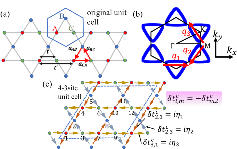
Figure 1: (a) Tight-binding model of the kagome lattice model. (b) FS of the 3-site kagome model at $n=5.0$. (c) The $3\bm{Q}$ cLC $\bm{\eta}=(\eta,\eta,\eta)/\sqrt{3}$ depicted in the kagome lattice.

When the nonzero wave vectors ${{\bm{q}}}_{n}$ of BO or cLC emerge in kagome lattice, the translational symmetry of the system is violated. In particular, by $3\bm{Q}$ order that three ${{\bm{q}}}_{n}$ coexist, the unit cell expands to 12 sites. Fig. 1 (c) shows the $3\bm{Q}$ current order $\bm{\eta}=(\eta_{1},\eta_{2},\eta_{3})$. We assign $\delta t_{i,j}^{c}=i\eta_{1}$  $[\delta t_{i,j}^{c}=-i\eta_{1}]$ for $(l,m)=(1,2),(2,4),(4,5),(5,1)$ $[(l,m)=(7,8),(8,10),(10,11),(11,7)]$, $\delta t_{i,j}^{c}=i\eta_{2}$  $[\delta t_{i,j}^{c}=-i\eta_{2}]$ for $(l,m)=(2,3),(3,11),(11,12),(12,2)$$[(l,m)=(5,6),(6,8),(8,9),(9,5)]$, and $\delta t_{i,j}^{c}=i\eta_{3}\ [\delta t_{i,j}^{c}=-i\eta_{3}]$ for $(l,m)=(4,6),(6,10),(10,12),(12,4)$$[(l,m)=(1,3),(3,7),(7,9),(9,1)]$. Here $\delta t^{c}_{i,j}$ is the purely imaginary ($(\delta t_{i,j}^{c})^{*}=-\delta t_{i,j}^{c}$) symmetry breaking term of the hopping integral, which is odd parity ($\delta t^{c}_{i,j}=-\delta t^{c}_{j,i}$) [35].

The Hamiltonian with the current order is given by

$$\hat{H}=\sum_{{{\bm{k}}},l,m}h_{lm}({{\bm{k}}})c^{\dagger}_{{{\bm{k}}},l}c_{{{\bm{k}}},m},$$ (1)

where $h_{lm}({{\bm{k}}})$ is the Fourier transformation of $t_{i,j}=t^{(0)}_{i,j}+\delta t^{c}_{i,j}$. The hopping integral is constructed with the original hopping integral $t^{(0)}_{i,j}$ and the current order $\delta t^{c}_{i,j}$. $l$ and $m$ denote the site number within the unit cell, $l,m=1\sim 12$. We use a index $i=\{\alpha,l\}$, where $\alpha$ denotes the unit cell. We introduce the notation ${{\bm{R}}}_{i}={{\bm{R}}}_{\alpha}+{{\bm{r}}}_{l}$ to designate the position of atoms, where ${{\bm{R}}}_{\alpha}$ is the position of the unit cell and ${{\bm{r}}}_{l}$ is the relative position of the atom within the unit cell. In the 12-site kagome lattice model, the FS folds, and the M and $\Gamma$ points in the lattice become equivalent. Therefore, the wave vector of the cLC order is ${{\bm{q}}}_{n}=\bm{0}$ for $n=1,2,3$ within folded BZ.

Here, we introduce the form factor of the cLC, which is given by the Fourier transformation of $\delta t^{c}_{i,j}$ shown in Fig. 1 (c). In the 3-site kagome lattice model, the cLC form factor between the nearest site $S$ and site $S^{\prime}$ ($S,S^{\prime}=A,B,C$) is given as blue$f_{SS^{\prime}}^{{{\bm{q}}}_{n}}({{\bm{k}}})=2\sin({{\bm{k}}}\cdot\bm{a}_{SS^{\prime}})$, where inter-site vector $\bm{a}_{SS^{\prime}}$ and the wavevector ${{\bm{q}}}_{n}$ are shown in Fig. 1 (a) and (b), respectively. Here, $n=1,2,3$ for $\left\{S,S^{\prime}\right\}=\left\{A,B\right\},\left\{B,C\right\},\left\{C,A\right\}$, respectively. The set of the current order functions is given by $(\eta_{1}f_{AB},\eta_{2}f_{BC},\eta_{3}f_{CA})$, where $\eta_{n}$ is the nth cLC order parameter. A more detailed explanation is presented in Ref. [20]. Hereafter, we set $\eta_{1}=\eta_{2}=\eta_{3}=\eta$ in the numerical study. We can also present the cLC form factor in the 12-site model, ${\tilde{f}}_{lm}(k)$, where $l,m=1\sim 12$ [12]. For example, ${\tilde{f}}_{12}({{\bm{k}}})=ie^{-i\bm{k}\cdot\bm{a}_{12}}$. In this representation, the cLC order wavevector becomes uniform $({{\bm{q}}}=\bm{0})$, so the incoming and outgoing momenta of ${\tilde{f}}_{lm}({{\bm{k}}})$ are the same. Here, we introduce the $12\times 12$ matrix expression of the current order function $[{\hat{C}}_{{{\bm{k}}}}]_{l,m}\equiv{\tilde{f}}_{l,m}({{\bm{k}}})$, which is convenient in the present numerical study. Here, $[{\hat{C}}_{{{\bm{k}}}}]_{l,m}\neq 0$ only when $(l,m)$ is the pair of the nearest sublattice.

The $3\bm{Q}$-cLC form factor of kagome metals is derived microscopically from the analysis of the DW equation with the BO fluctuation exchange term as the kernel, as shown in ref. [35]. The $\delta t_{i,j}$ derived in ref. [35] has the same absolute value for all nearest-neighbor bonds $(i,j)$, meaning $|\delta t_{i,j}^{c}|=\eta$. It is worth noting that the $\delta t_{i,j}$ derived in ref. [35] also has long-range components, but for simplicity in this paper, we consider only the nearest-neighbors.

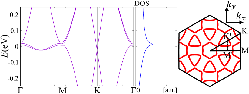
Figure 2: Band structure, DOS, and FS of the 12-site kagome lattice model with $\eta=0.1$.

We show the band structure, density of states (DOS), and FS of the 12-site kagome lattice model that cLC order is introduced at $\eta=0.1$ in Fig 2. In the 12-site kagome lattice, vHS exists at the M-point, leading to a large DOS. The introduction of cLC order resolves the strong degeneracy near the M point, while the large magnitude of the DOS remains.

Next, to calculate the spontaneous charge current in the cLC phase, we introduce the current order operator from Heisenberg eq. $\dot{n}_{i}=-i[n_{i},H]=-i\left(\sum_{j}t_{i,j}c_{i}^{\dagger}c_{j}-\sum_{j}t_{j,i}c_{j}^{\dagger}c_{i}\right)$. Then, the current operator is derived from the continuity equation as

$$j_{i,j}=-i(t_{i,j}c^{\dagger}_{i}c_{j}-(i\leftrightarrow j)).$$ (2)

By taking the expectation value with respect to grand canonical ensemble, the current from site $j$ to site $i$ is given as

$$J_{i,j}=\langle j_{i,j}\rangle=it_{i,j}g_{j,i}-(i\leftrightarrow j),$$ (3)

where the equal time Green function is given as $g_{i,j}=\lim_{u\rightarrow-0}\langle Tc^{\dagger}_{i}(u)c_{j}(0)\rangle$. $\langle\cdots\rangle$ represents the mean value for the grand canonical ensemble. The Green function in momentum representation is

$$G_{l,m}({{\bm{k}}},i\epsilon_{n})=((i\epsilon_{n}+\mu)\hat{\bm{1}}-\hat{h}({{\bm{k}}}))^{-1}_{l,m}.$$ (4)

We derive the equal time Green function by the Fourier transform of Eq. (4) as $g_{i,j}=T\sum_{n,{{\bm{k}}}}G_{l,m}({{\bm{k}}},i\epsilon_{n})e^{i{{\bm{k}}}\cdot({{\bm{R}}}_{\alpha}-{{\bm{R}}}_{\beta})}e^{i\epsilon_{n}\delta}$. Note that the factor $e^{i\epsilon_{n}\delta}$ is not necessary for $l\neq m$. $\epsilon_{n}=(2n-1)\pi T$ is the fermion Matsubara frequency. Here n is integer.

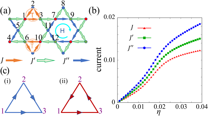
Figure 3: (a) Obtained distribution of the charge currents. Here, $J(J^{\prime\prime})$ is the current along the triangular (hexagonal) loop where the direction of each cLC order is aligned. The current on other bonds is given as $J^{\prime\prime}$ (b) Obtained currents as a functions of $\eta$. (c) 3-site cluster models with different cLC orders. The circulating current in $\rm(\hskip 1.79993pti\hskip 1.79993pt)$ differs from that in $\rm(\hskip 0.80002ptii\hskip 0.80002pt)$; see the text.

Analysis of spontaneous current - Now, we present the results of the current distribution induced by the cLC orders. Fig. 3 (a) illustrates the real-space current distribution within the kagome lattice. The obtained currents as a function of $\eta$ are shown in Fig. 3 (b) ($T=2.5$meV, $n=5.0$) . As $\eta$ increases, the difference in the magnitude of the currents is enlarged.

To understand the obtained nontrivial relation between $J_{i,j}$ and $\delta t_{i,j}$, here we analyze a simple 3-site cluster model with cLC order oriented in different directions. Fig. 3 (c) represents two 3-site cluster models, $\rm(\hskip 1.79993pti\hskip 1.79993pt)$ and $\rm(\hskip 0.80002ptii\hskip 0.80002pt)$. In the case of $\rm(\hskip 1.79993pti\hskip 1.79993pt)$, $\delta t^{c}_{ij}$ is given as $\delta t^{c}_{21}=\delta t^{c}_{31}=\delta t^{c}_{32}=i\eta$. The current $J^{1}_{1,2}$ that flows in model $\rm(\hskip 1.79993pti\hskip 1.79993pt)$ is derived as $J^{1}_{1,2}=-2\eta(t^{2}+\eta^{2})A$, where $A=T\sum_{n}\left[(i\epsilon_{n}+\mu)^{3}+3(t^{2}+\eta^{2})(i\epsilon_{n}+\mu)+2t(t^{2}+\eta^{2})\right]^{-1}$. In the case of $\rm(\hskip 1.79993ptii\hskip 1.79993pt)$, $\delta t^{c}_{ij}$ is given as $\delta t^{c}_{12}=\delta t^{c}_{23}=\delta t^{c}_{31}=i\eta$. Then, the current $J^{2}_{1,2}$ is caluculated as $J^{2}_{1,2}=6\eta(t^{2}-\frac{\eta^{2}}{3})B$, where $B=T\sum_{n}\left[(i\epsilon_{n}+\mu)^{3}+3(t^{2}+\eta^{2})(i\epsilon_{n}+\mu)\right.$$\left.+2t(t^{2}-3\eta^{2})\right]^{-1}$. Thus, different magnitudes of current emerge even when the same order parameter $\eta$ is provided in three directions ${{\bm{q}}}_{1},{{\bm{q}}}_{2},{{\bm{q}}}_{3}$. It holds that $|J_{12}^{m}|=|J_{23}^{m}|=|J_{31}^{m}|$ for each m = 1,2. In the case that $|a|\ll|t|$, $|J_{12}^{2}|=3|J_{12}^{1}|$ holds. In this finite site model, the current converges to zero at $T=0$ and $T\rightarrow\infty$.

The mathematical reason for the difference in current between $\rm(\hskip 1.79993pti\hskip 1.79993pt)$ and $\rm(\hskip 1.79993ptii\hskip 1.79993pt)$ is that the $J_{1,2}$ given in Eq. (3) contributes not only to $\delta t_{1,2}^{c}$ but also to $\delta t_{1,3}^{c}$, $\delta t_{2,3}^{c}$, which are included in $g_{1,2}$. When the phases of $\delta t_{i,j}^{c}$ on the closed loop are aligned, i.e., $\delta t_{1,2}^{c}=\delta t_{2,3}^{c}=\delta t_{3,1}^{c}$, the induced current $|J_{i,j}|$ becomes the largest. This consideration leads us to understand why $J$ ,$J^{\prime}$, and $J^{\prime\prime}$ are different in kagome metals as shown in Fig. 3(a)-(b).

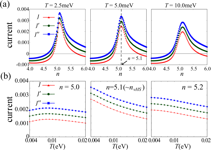
Figure 4: (a) $n$-dependence of the currents at $T=2.5-10.0$ meV. (b) T-dependence of the currents at $n=5.0-5.2$.

Next, we analyze the filling and temperature dependence of the current. The filling dependence of the current is depicted in Fig. 4 (a). It shows that the current reaches a maximum near the vHS filling. Fig. 4 (b) illustrates the temperature dependence of the current. The magnitude of the current increases at the low-tempratures, with a pronounced increase near the vHS filling.

Susceptibility of the current - Next stage, we consider susceptibility that describes the behavior of the current. First, we expand the Green function in terms of the order parameter $\eta$ as $\hat{G}\left({{\bm{k}}},i\epsilon_{n}\right)\sim\hat{G}^{(0)}\left({{\bm{k}}},i\epsilon_{n}\right)+\hat{G}^{(0)}\left({{\bm{k}}},i\epsilon_{n}\right)\eta{\hat{C}}_{{{\bm{k}}}}\hat{G}^{(0)}\left({{\bm{k}}},i\epsilon_{n}\right)$, where $\hat{G}^{(0)}({{\bm{k}}},i\epsilon_{n})$ is the Green function with $\eta=0$. The contribution from the term $\hat{G}^{(0)}({{\bm{k}}},i\epsilon_{n})\eta{\hat{C}}_{{{\bm{k}}}}\hat{G}^{(0)}({{\bm{k}}},i\epsilon_{n})$ to the current is dominant. The diagramatic representations of this term is shown in Fig. 5 (a). Meanwhile, the static irreducible susceptibility is

$$\hat{\chi}^{J-\eta}_{lml^{\prime}m^{\prime}}({{\bm{q}}})$$

$$=-\frac{T}{N}\sum_{{{\bm{k}}},n}G^{(0)}_{ll^{\prime}}({{\bm{k}}}+{{\bm{q}}},i\epsilon_{n})G^{(0)}_{m^{\prime}m}({{\bm{k}}},i\epsilon_{n}).$$ (5)

As an example of form factor, $[\hat{C}_{{{{\bm{k}}}}}]_{12}=ie^{i{{\bm{k}}}\cdot\bm{a}_{AB}}$, and $[\hat{C}_{{{\bm{k}}}}]_{21}=-ie^{i{{\bm{k}}}\cdot\bm{a}_{BA}}$. Thus, at ${{\bm{k}}}=0$ which corresponds to $\Gamma$ point, $[\hat{C}_{\bm{0}}]_{12}=i$ holds. Here, we recall that sites $1$,$4$,$7$, and $10$ belong to the A site, while site $2$,$5$,$8$, and $11$ belong to B site. In the case of the 12-site kagome lattice model, the form factor exhibits the largest value at the $\Gamma$ point. Therefore, after approximating it as $[\hat{C}_{{{\bm{k}}}}]_{lm}\sim[\hat{C}_{\bm{0}}]_{lm}$, it is possible to perform the following transformations as

$$J_{1,2} \propto T\sum_{n,l,m,{{\bm{k}}}}[G^{(0)}]_{1,l}\eta[\hat{C}_{\bm{0}}]_{l,m}[G^{(0)}]_{m,2}e^{i{{\bm{k}}}\cdot({{\bm{R}}}_{\alpha}-{{\bm{R}}}_{\beta})}$$ (6)

$$\sim\sum_{l,m=1-12}\chi_{12,lm}^{J-\eta}(\bm{0})[\hat{C}_{\bm{0}}]_{lm}\eta.$$

Importantly, $\chi_{12,lm}^{J-\eta}(\bm{0})$ becomes large when $\left\{l,m\right\}=\left\{1,2\right\},\left\{4,5\right\},\left\{7,8\right\},\left\{10,11\right\}$, by reflecting the sublattice interference of the pure-type FS. If one puts a restriction $\left\{l,m\right\}=\left\{1,2\right\}$, $J_{1,2}$ in Eq. (6) is proportional to $\chi_{12,12}^{J-\eta}-\chi_{12,21}^{J-\eta}$.

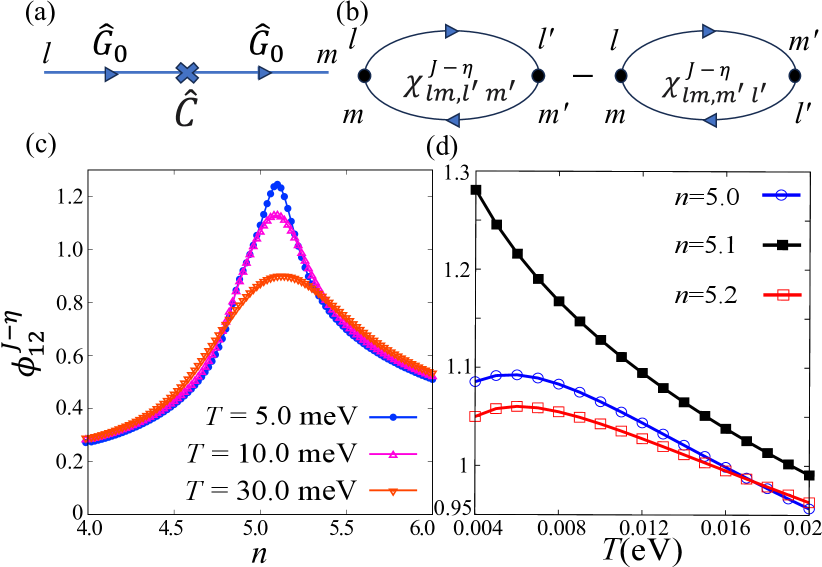
Figure 5: (a) Diagrammatic representation of the first-order term $\left(\hat{G}^{(0)}\eta\hat{C}\hat{G}^{(0)}\right)_{m,l}$. (b) Diagrammatic representation of the sum of susceptibility $\chi_{lml^{\prime}m^{\prime}}^{J-\eta}-\chi_{lmm^{\prime}l^{\prime}}^{J-\eta}$. (c) Filling dependence of $\phi_{12}^{J-\eta}$ at $T=5.0,10,30$ meV. (d) Temperature dependence of $\phi_{12}^{J-\eta}$ at $n=5.0-5.2$.

Figure 5 (b) represents diagrammatic representations of $\chi_{1l,m2}^{J-\eta}(\bm{0})$. Taking account of the form factors depicted in Fig. 1 (c), the summation of contributions from $\left\{l,m\right\}=\left\{1,2\right\}$, $\left\{4,5\right\}$, $\left\{7,8\right\}$, and $\left\{10,11\right\}$ leads to $\phi_{12}^{J-\eta}=[\chi_{12,12}^{J-\eta}-\chi_{12,21}^{J-\eta}+\chi_{12,42}^{J-\eta}-\chi_{12,24}^{J-\eta}+\chi_{12,45}^{J-\eta}-\chi_{12,54}^{J-\eta}+\chi_{12,14}^{J-\eta}-\chi_{12,41}^{J-\eta}]-[\chi_{12,78}^{J-\eta}-\chi_{12,87}^{J-\eta}+\chi_{12,10\ 8}^{J-\eta}-\chi_{12,8\ 10}^{J-\eta}+\chi_{12,10\ 11}^{J-\eta}-\chi_{12,11\ 10}^{J-\eta}+\chi_{12,7\ 10}^{J-\eta}-\chi_{12,10\ 7}^{J-\eta}]$.

The filling and temperature dependence of $\phi_{12}^{J-\eta}$ are shown respectively in Fig. 5 (c) and (d). $\phi_{12}^{J-\eta}$ reaches its maximum value at the vHS filling, with a notable increase in the low temperature regime. In kagome metals, $\phi_{12}^{J-\eta}$ significantly increases at low temperatures for $n\sim n_{VHS}$. Analytically, at vHS filling, $\phi_{12}^{J-\eta}\propto 1/E_{0}\left(\ln E_{0}/T\right)^{2}+\chi_{0c}$ when $E_{0}\sim 0.1$[eV] is the energy range where the vHS bandstructure is well described by the quadratic expression, as discussed in Ref. [19]. Here, $\chi_{0c}$ is the constraint susceptibility, which excludes the contribution for $|E|<E_{0}$ from Eq. (5), which is defined in SM in Ref. [37]. This temperature dependence is attributed to the singularity at vHS in the kagome lattice model, in stark contrast to usual metals, where $\phi_{12}^{J-\eta}$ remains constant.

Effect of self-energy - In addition, we analyze how the current is modified by the self-energy. Fig. 6 (a) shows the filling dependence of the current in the presence of self-energy. Fig. 6 (b) shows the obtained damping rate $\gamma$ dependence of current. As $\gamma$ increases, the current is gradually suppressed.

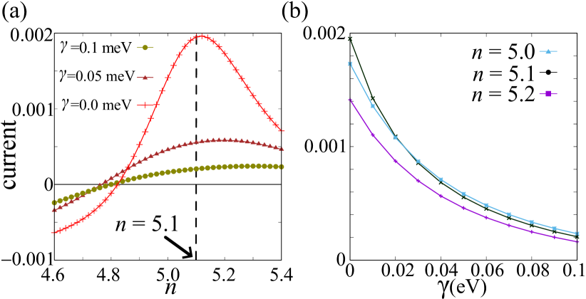
Figure 6: (a) Filling dependence of the current $J^{\rm min}=\min\{J,J^{\prime},J^{\prime\prime}\}$ for various $\gamma$. (b) $\gamma$ dependence of $J^{\rm min}$ for $n=5.0-5.2$.

Summary and discussions - In this letter, we employed the Green function method to calculate the real-space current distribution in the $3{\bm{Q}}$-cLC phase of kagome metal. The obtained magnitude of $J_{i,j}$ strongly depends on the nearest sites ($i,j$) even when $|\delta t_{i,j}|$ is constant for any bonds. The obtained $J_{i,j}$ becomes large near the vHS filling, while it is suppressed when considering self-energy. Interestingly, $J_{i,j}$ exhibits the logarithmic divergence behavior at low temperatures for $n\sim n_{\rm vHS}$. The present study provides useful information for local electronic state measurements, such as the site-selective NMR and STM experiments.

We have employed the Green function method to calculate $J_{i,j}$. Based on this method, one can calculate the current by including the beyond-mean-field electron correlations, such as the self-energy and the VCs. This is a great advantage of the present method.

- [1] Yu-Xiao Jiang, Jia-Xin Yin, M. Michael Denner, Nana Shumiya, Brenden R. Ortiz, Gang Xu, Zurab Guguchia, Junyi He, Md Shafayat Hossain, Xiaoxiong Liu, Jacob Ruff, Linus Kautzsch, Songtian S. Zhang, Guoqing Chang, Ilya Belopolski, Qi Zhang, Tyler A. Cochran, Daniel Multer, Maksim Litskevich, Zi-Jia Cheng, Xian P. Yang, Ziqiang Wang, Ronny Thomale, Titus Neupert, Stephen D. Wilson, Zahid Hasan Unconventional chiral charge order in kagome superconductor KV3Sb5, Nat. Mat. 20, 1353-1357 (2021).
- [2] Hong Li, He Zhao, Brenden R. Ortiz, Takamori Park, Mengxing Ye, Leon Balents, Ziqiang Wang, Stephen D. Wilson, Ilija Zeljkovic Rotational symmetry breaking in the normal state of a kagome superconductor KV3Sb5, Nat. Phys. 18, 265 (2022)
- [3] B. R. Ortiz, L. C. Gomes, J. R. Morey, M. Winiarski, M. Bordelon, J. S. Mangum, I. W. H. Oswald, J. A. Rodriguez-Rivera, J. R. Neilson, S. D. Wilson, E. Ertekin, T. M. McQueen, and E. S. Toberer, New kagome prototype materials: discovery of , and , Phys. Rev. Materials 3, 094407 (2019).
- [4] B. R. Ortiz, S. M. L. Teicher, Y. Hu, J. L. Zuo, P. M. Sarte, E. C. Schueller, A. M. M. Abeykoon, M. J. Krogstad, S. Rosenkranz, R. Osborn, R. Seshadri, L. Balents, J. He, and S. D. Wilson, : A Topological Kagome Metal with a Superconducting Ground State, Phys. Rev. Lett. 125, 247002 (2020).
- [5] F. H. Yu, D. H. Ma, W. Z. Zhuo, S. Q. Liu, X. K. Wen, B. Lei, J. J. Ying, and X. H. Chen, Unusual competition of superconductivity and charge-density-wave state in a compressed topological kagome metal, Nat. Commun. 12, 3645 (2021).
- [6] K. Y. Chen, N. N. Wang, Q. W. Yin, Y. H. Gu, K. Jiang, Z. J. Tu, C. S. Gong, Y. Uwatoko, J. P. Sun, H. C. Lei, J. P. Hu, and J.-G. Cheng, Double Superconducting Dome and Triple Enhancement of in the Kagome Superconductor under High Pressure, Phys. Rev. Lett. 126, 247001 (2021).
- [7] B. R. Ortiz, P. M. Sarte, E. M. Kenney, M. J. Graf, S. M. L. Teicher, R. Seshadri, and S. D. Wilson, Superconductivity in the kagome metal , Phys. Rev. Materials 5, 034801 (2021).
- [8] L. Nie, K. Sun, W. Ma, D. Song, L. Zheng, Z. Liang, P. Wu, F. Yu, J. Li, M. Shan, D. Zhao, S. Li, B. Kang, Z. Wu, Y. Zhou, K. Liu, Z. Xiang, J. Ying, Z. Wang, T. Wu, and X. Chen, Charge-density-wave-driven electronic nematicity in a kagome superconductor, Nature 604, 59 (2022).
- [9] Y. Xu, Z. Ni, Y. Liu, B. R. Ortiz, S. D. Wilson, B. Yan, L. Balents, and L. Wu, Universal three-state nematicity and magneto-optical Kerr effect in the charge density waves in AV3Sb5 (A=Cs, Rb, K), arXiv:2204.10116.
- [10] H. Li, H. Zhao, B. R. Ortiz, T. Park, M. Ye, L. Balents, Z. Wang, S. D. Wilson, and I. Zeljkovic, Rotation symmetry breaking in the normal state of a kagome superconductor KV3Sb5, Nat. Phys. 18, 265 (2022).
- [11] T. Asaba, A. Onishi, Y. Kageyama, T. Kiyosue, K. Ohtsuka, S. Suetsugu, Y. Kohsaka, T. Gaggl, Y. Kasahara, H. Murayama, K. Hashimoto, R. Tazai, H. Kontani, B. R. Ortiz, S. D. Wilson, Q. Li, H. -H. Wen, T. Shibauchi, Y. Matsuda, Evidence for an odd-parity nematic phase above the charge density wave transition in kagome metal CsV3Sb5. accepted for publication in Nat. Phys. (arXiv:2309.16985).
- [12] R. Tazai, Y. Yamakawa, and H. Kontani, Drastic magnetic-field-induced chiral current order and emergent current-bond-field interplay in kagome metals, accepted for publication in Proceedings of the National Academy of Sciences (PNAS) (available at https://arxiv.org/abs/2303.00623).
- [13] arXiv:2305.18087
- [14] M. M. Denner, R. Thomale, and T. Neupert, Analysis of Charge Order in the Kagome Metal (), Phys. Rev. Lett. 127, 217601 (2021).
- [15] Y.-P. Lin and R. M. Nandkishore, Complex charge density waves at Van Hove singularity on hexagonal lattices: Haldane-model phase diagram and potential realization in the kagome metals AV3Sb5 (A = K, Rb, Cs), Phys. Rev. B 104, 045122 (2021).
- [16] M. L. Kiesel, C. Platt, and R. Thomale, Unconventional Fermi Surface Instabilities in the Kagome Hubbard Model, Phys. Rev. Lett. 110, 126405 (2013).
- [17] W.-S. Wang, Z.-Z. Li, Y.-Y. Xiang, and Q.-H. Wang, Competing electronic orders on kagome lattices at van Hove filling, Phys. Rev. B 87, 115135 (2013).
- [18] H. D. Scammell, J. Ingham, T. Li, and O. P. Sushkov, Chiral excitonic order from twofold van Hove singularities in kagome metals, Nat. Commun. 14, 605 (2023)
- [19] T. Park, M. Ye, and L. Balents, Electronic instabilities of kagome metals: Saddle points and Landau theory, Phys. Rev. B 104, 035142 (2021).
- [20] R. Tazai, Y. Yamakawa, S. Onari, and H. Kontani, Mechanism of exotic density-wave and beyond-Migdal unconventional superconductivity in kagome metal AV3Sb5 (A = K, Rb, Cs), Sci. Adv. 8, eabl4108 (2022).
- [21] S. Onari, Y. Yamakawa, and H. Kontani, Phys. Rev. Lett. 112, 187001 (2014).
- [22] S. Onari, Y. Yamakawa, and H. Kontani, Phys. Rev. Lett. 116, 227001 (2016).
- [23] Y. Yamakawa, S. Onari and H. Kontani, Phys. Rev. X 6, 021032 (2016).
- [24] S.-Y. Yang, Y. Wang, B. R. Ortiz, D. Liu, J. Gayles, E. Derunova, R. Gonzalez-Hernandez, L. mejkal, Y. Chen, S. S. P. Parkin, S. D. Wilson, E. S. Toberer, T. McQueen, and M. N. Ali, Giant, unconventional anomalous Hall effect in the metallic frustrated magnet candidate, KV3Sb5, Sci. Adv. 6, eabb6003 (2020).
- [25] F. H. Yu, T. Wu, Z. Y. Wang, B. Lei, W. Z. Zhuo, J. J. Ying, and X. H. Chen, Concurrence of anomalous Hall effect and charge density wave in a superconducting topological kagome metal, Phys. Rev. B 104, L041103 (2021).
- [26] C. Mielke, D. Das, J.-X. Yin, H. Liu, R. Gupta, Y.-X. Jiang, M. Medarde, X. Wu, H. C. Lei, J. Chang, P. Dai, Q. Si, H. Miao, R. Thomale, T. Neupert, Y. Shi, R. Khasanov, M. Z. Hasan, H. Luetkens, and Z. Guguchia, Time-reversal symmetry-breaking charge order in a kagome superconductor, Nature 602, 245 (2022).
- [27] R. Khasanov, D. Das, R. Gupta, C. Mielke, M. Elender, Q. Yin, Z. Tu, C. Gong, H. Lei, E. T. Ritz, R. M. Fernandes, T. Birol, Z. Guguchia, and H. Luetkens, Time-reversal symmetry broken by charge order in , Phys. Rev. Research 4, 023244 (2022).
- [28] Z. Guguchia, C. Mielke, D. Das, R. Gupta, J.-X. Yin, H. Liu, Q. Yin, M. H. Christensen, Z. Tu, C. Gong, N. Shumiya, M. S. Hossain, T. Gamsakhurdashvili, M. Elender, P. Dai, A. Amato, Y. Shi, H. C. Lei, R. M. Fernandes, M. Z. Hasan, H. Luetkens, and R. Khasanov, Tunable unconventional kagome superconductivity in charge ordered RbV3Sb5 and KV3Sb5, Nat. Commun. 14, 153 (2023).
- [29] C. Guo, G. Wagner, C. Putzke, D. Chen, K. Wang, L. Zhang, M. G. Amigo, I. Errea, M. G. Vergniory, C. Felser, M. H. Fischer, T. Neupert, and P. J. W. Moll, Correlated order at the tipping point in the kagome metal CsV3Sb5, arXiv:2304.00972.
- [30] F. D. M. Haldane, Model for a Quantum Hall Effect without Landau Levels: Condensed-Matter Realization of the ”Parity Anomaly”, Phys. Rev. Lett. 61, 2015 (1988).
- [31] I. Affleck and J. B. Marston, Large-n limit of the Heisenberg-Hubbard model: Implications for high- superconductors, Phys. Rev. B 37, 3774(R) (1988).
- [32] C. M. Varma, Theory of the pseudogap state of the cuprates, Phys. Rev. B 73, 155113 (2006).
- [33] W. H. P. Nielsen, W. A. Atkinson, and B. M. Andersen, Signatures of orbital loop currents in the spatially resolved local density of states, Phys. Rev. B 86, 054510 (2012).
- [34] R. Tazai, Y. Yamakawa, and H. Kontani, Emergence of charge loop current in the geometrically frustrated Hubbard model: A functional renormalization group study, Phys. Rev. B 103, L161112 (2021).
- [35] R. Tazai, Y. Yamakawa, and H. Kontani, Charge-loop current order and Z3 nematicity mediated by bond-order fluctuations in kagome metals, Nat. Commun. 14, 7845 (2023).
- [36] H. Kontani, Y. Yamakawa, R. Tazai, and S. Onari, Odd-parity spin-loop-current order mediated by transverse spin fluctuations in cuprates and related electron systems, Phys. Rev.Research 3, 013127 (2021)
- [37] M. Tsuchiizu, Yusuke Ohno, Seiichiro Onari, and H. Kontani Orbital Nematic Instability in the Two-Orbital Hubbard Model: Renormalization-Group + Constrained RPA Analysis, Phys. Rev. B 93, 155148.
- [38] H. Kontani, R. Tazai, Y. Yamakawa, and S. Onari, Unconventional density waves and superconductivities in Fe-based superconductors and other strongly correlated electron systems, Adv. Phys. 70, 355 (2021).
- [39] R. Tazai, S. Matsubara, Y. Yamakawa, S. Onari, and H. Kontani, Rigorous formalism for unconventional symmetry breaking in Fermi liquid theory and its application to nematicity in FeSe, Phys. Rev. B 107, 035137 (2023).
- [40] F. Grandi, A. Consiglio, M. A. Sentef, R. Thomale, and D. M. Kennes, Theory of nematic charge orders in kagome metals, Phys. Rev. B 107, 155131 (2023)
- [41] X. Wu, T. Schwemmer, T. Müller, A. Consiglio, G. Sangiovanni, D. Di Sante, Y. Iqbal, W. Hanke, A. P. Schnyder, M. M. Denner, M. H. Fischer, T. Neupert, and R. Thomale, Nature of Unconventional Pairing in the Kagome Superconductors (), Phys. Rev. Lett. 127, 177001 (2021).
- [42] J. Huang, Y. Yamakawa, R. Tazai, and H. Kontani, Odd-parity intra-unit-cell bond-order and induced nematicity in kagome metal CsTi3Bi5 driven by quantum interference mechanism, arXiv:2305.18093 (available at https://arxiv.org/abs/2305.18093).
- [43] A. V. Chubukov, M. Khodas, and R. M. Fernandes, Phys. Rev. X 6, 041045 (2016).
- [44] M. Tsuchiizu, K. Kawaguchi, Y. Yamakawa, and H. Kontani, Phys. Rev. B 97, 165131 (2018).
- [45] C. Guo, C. Putzke, S. Konyzheva, X. Huang, M. Gutierrez-Amigo, I. Errea, D. Chen, M. G. Vergniory, C. Felser, M. H. Fischer, T. Neupert, and P. J. W. Moll, Switchable chiral transport in charge-ordered Kagome metal CsV3Sb5, Nature 611, 461 (2022).
- [46] J. Luo, Z. Zhao, Y. Z. Zhou, J. Yang, A. F. Fang, H. T. Yang, H. J. Gao, R. Zhou, and G.-q. Zheng, Possible star-of-David pattern charge density wave with additional modulation in the kagome superconductor CsV3Sb5, npj Quantum Materials 7, 30 (2022).
- [47] M. H. Christensen, T. Biro, B. M. Andersen, and R. M. Fernandes, Loop currents in AV3Sb5 kagome metals: Multipolar and toroidal magnetic orders, Phys. Rev. B 106, 144504 (2022)