Jeans modelling of weakly flattened ellipsoidal systems

Abstract

In the homoeoidal expansion, a given ellipsoidally stratified density distribution, and its associated potential, are expanded in the (small) density flattening parameter $\eta$, and usually truncated at the linear order. The truncated density-potential pair obeys exactly the Poisson equation, and it can be interpreted as the first-order expansion of the original ellipsoidal density-potential pair, or as a new autonomous system. In the first interpretation, in the solutions of the Jeans equations the quadratic terms in $\eta$ must be discarded (“$\eta$-linear” solutions), while in the second (“$\eta$-quadratic”) all terms are retained. In this work we study the importance of the quadratic terms by using the ellipsoidal Plummer model and the Perfect Ellipsoid, which allow for fully analytical $\eta$-quadratic solutions. These solutions are then compared with those obtained numerically for the original ellipsoidal models, finding that the $\eta$-linear models already provide an excellent approximation of the numerical solutions. As an application, the $\eta$-linear Plummer model (with a central black hole) is used for the phenomenological interpretation of the dynamics of the weakly flattened and rotating globular cluster NGC 4372, confirming that this system cannot be interpreted as an isotropic rotator, a conclusion reached previously with more sophisticated studies.

1 Introduction

For their intrinsic simplicity in stellar dynamics, spherical models are of great utility both in theory and applications (e.g. Binney & Tremaine 2008, hereafter BT08; Bertin 2014; Ciotti 2021, hereafter C21). However, phenomena such as rotation can be studied properly only by allowing for some flattening in the density profile. Among the specific difficulties encountered in modelling non-spherical systems, the derivation of the gravitational potential is certainly a major one, and, apart from special cases in which the solution is known in explicit form, one must resort to time-consuming numerical integrations. In turn, if the potential is only known numerically, then also the Jeans equations must be solved numerically, making the exploration of the parameter space even more laborious. Fortunately, many real stellar systems are characterised by small deviations from spherical symmetry; examples of weakly flattened systems are, for instance, E1/E3 galaxies, and many Globular Clusters (e.g. Varri & Bertin 2012). For these systems, the technique of the homoeoidal expansion (Ciotti & Bertin 2005, hereafter CB05) provides an approximate, yet robust, and easy procedure to build one- and multi-component dynamical models (Ciotti et al. 2021, hereafter CMPZ21; see also Chapter 13 in C21, and references therein).

In practice, in the homoeoidal expansion method, a chosen ellipsoidally stratified density distribution, and the associated potential, are usually expanded and truncated at the linear order in terms of the density flattening $\eta$, therefore producing, thanks to the linearity of Poisson’s equation, an exact density-potential pair. Both the density and the potential are written as a spherical part plus a non-spherical term proportional to $\eta$; the non-spherical term, in turn, reduces to the product of the square of the cylindrical radius $R$ and a spherical function. This very specific structure allows for manageable solutions of the Jeans equations. Of course, the truncation at the linear order in $\eta$ of the original density-potential pair is only matter of convenience, as the linearity of the Poisson equation implies that, at any truncation order in $\eta$, the resulting truncated functions are an exact density-potential pair. However, increasing the order of truncation increases also the number of terms to be considered in the solution of the Jeans equations; therefore it is natural to ask how good the linear truncation already is, in order to save as much computational effort as possible, while maintaining a reasonable description of the original system.

A second closely related question arises when considering the solution of the Jeans equations even for the linearly truncated density-potential pair. In fact, the truncated density-potential pair can be seen in two different ways: as the first-order expansion of the ellipsoidal parent galaxy model in the limit of small flattening, or as an independent non-spherical system. In the first interpretation (“$\eta$-linear”), only linear terms in the flattening are retained in the solution of the Jeans equations; in the second interpretation (“$\eta$-quadratic”), the Jeans equations contain up to quadratic terms in the flattening. In previous works, only the first interpretation has been discussed; here we investigate the effects of including higher order $\eta$-terms in the solutions of the Jeans equations: it is quite obvious that the discarded terms, proportional to $\eta^{2}$ and depending on coordinates, are not necessarily small, and in principle in some regions of space they could be even larger than lower order terms.

In this paper we address these questions, and compare the solutions of the Jeans equations of the original ellipsoidal model (hereafter “full solution”) with their $\eta$-linear and $\eta$-quadratic expansions, in order to quantify the performance of the homoeoidal expansion method. For this study, we consider two simple ellipsoidal models: the Perfect Ellipsoid (de Zeeuw & Lynden-Bell 1985, hereafter ZL85) and the ellipsoidal Plummer (1911, hereafter P11) model, to which a central black hole (BH) is added. For these, the $\eta$-quadratic (and so the $\eta$-linear) solutions can be evaluated analytically in terms of elementary functions. In particular, for each model we compare the two expanded solutions with that recovered numerically for the original model. We find that the $\eta$-linear approximation suffices to provide excellent agreement with the numerical solution, for small but realistic values of $\eta$. We then exploit this result by building an $\eta$-linear Plummer model for the Globular Cluster (GC) NGC 4372, to investigate the relation between flattening and ordered rotation. This GC is a natural candidate for an exploratory study with our method, since its density profile is well described by the Plummer model (see Kacharov et al. 2014), and its flattening is sufficiently low for applicability of the $\eta$-linear modeling. Another motivation for this application is given by the remarkable property of homoeoidally expanded systems of having a streaming velocity field that scales as $\sqrt{\eta}$, increases linearly with radius in the central regions, and decreases outward after a maximum; these features are noticeably similar to those commonly observed, or adopted in a phenomenological description, for the rotation curves of GCs. In agreement with previous results obtained with more sophisticated methods (e.g. Varri & Bertin 2012; Bianchini et al. 2013; Jeffreson et al. 2017), our simple modelling excludes the possibility that NGC 4372 is an isotropic rotator, and we suggest instead that the observed rotational structure is possibly due to the presence of a rotating stellar substructure.

The paper is organised as follows. In Section 2 we summarize the technical details and main formulae of the homoeoidal expansion. In Section 3, we set up and discuss the $\eta$-linear and $\eta$-quadratic solutions of the associated Jeans equations. In Section 4, the main structural and dynamical properties of the two families of models are presented, with a detailed analysis of the solutions of the Jeans equations generated by the two different interpretations. Finally, in Section 5 we present a simple application of the $\eta$-linear modelling to the GC NGC 4372.

2 The Homoeoidal Expansion

We recall the main properties of the homoeoidal expansion. Let ${\bf x}=(x,y,z)$, and consider a mass density distribution $\rho({\bf x})$ of total mass $M$ stratified on ellipsoidal surfaces

$$m^{2}\equiv\frac{x^{2}}{a^{2}}+\frac{y^{2}}{b^{2}}+\frac{z^{2}}{c^{2}}=\tilde{x}^{2}+\frac{\tilde{y}^{2}}{q_{y}^{2}}+\frac{\tilde{z}^{2}}{q_{z}^{2}}\hskip 0.56905pt,$$ (1)

with $a\geq b\geq c>0$, $\tilde{x}\equiv x/a$, $\tilde{y}\equiv y/a$, $\tilde{z}\equiv z/a$, $q_{y}\equiv b/a$, and $q_{z}\equiv c/a$. For $q_{y}=q_{z}=1$, the distribution is spherically symmetric, the oblate case corresponds to $q_{y}=1$ and $0<q_{z}<1$, and the prolate to $0<q_{y}=q_{z}<1$. We write

$$\frac{\rho({\bf x})}{\rho_{\rm n}}=\frac{\tilde{\rho}(m)}{q_{y}q_{z}}\hskip 0.56905pt,\qquad\rho_{\rm n}\equiv\frac{M}{4\pi a^{3}}.$$ (2)

Notice that $\tilde{\rho}$, as a function of its argument, is independent of $q_{y}$ and $q_{z}$, and it can be identified with the spherical member of the ellipsoidal family. Notice that the presence of the coefficient $q_{y}q_{z}$ at the denominator in equation (2) guarantees that $M$ is the mass of the model independently of the flattening, and, from equation (2), the mass within the ellipsoid $m$ reads

$$\frac{M(m)}{M}=\int_{0}^{m}\tilde{\rho}(t)\hskip 1.13809ptt^{2}dt.$$ (3)

The (relative) potential associated with the density distribution in equation (2) is given by

$$\frac{\Psi({\bf x})}{\Psi_{\rm n}}=\frac{1}{4}\bigintsss_{\hskip 1.13809pt0}^{\infty}\frac{F[m({\bf x}\hskip 0.56905pt,u)]}{\sqrt{\hskip 0.56905ptD(u)\hskip 0.85358pt}}\hskip 0.85358ptdu,\qquad\,\,F(m)\equiv 2\int_{m}^{\infty}\tilde{\rho}(t)\hskip 0.85358ptt\hskip 0.28453ptdt,$$ (4)

(e.g. BT08; see also exercise 2.12 in C21), where $\Psi_{\rm n}\equiv GM/a$, $G$ is the gravitational constant,

$$D(u)\equiv(1+u)\hskip 0.56905pt(q_{y}^{2}+u)\hskip 0.56905pt(q_{z}^{2}+u)\hskip 0.85358pt,$$ (5)

and

$$m^{2}({\bf x}\hskip 0.85358pt,u)\equiv\frac{\tilde{x}^{2}}{1+u}+\frac{\tilde{y}^{2}}{q_{y}^{2}+u}+\frac{\tilde{z}^{2}}{q_{z}^{2}+u}\hskip 0.85358pt.$$ (6)

Finally (Roberts 1962), the gravitational self-energy $W$ can be written as

$$\frac{W}{M\Psi_{\rm n}}=-\hskip 1.13809pt\frac{\varw_{1}+q_{y}^{2}\hskip 1.13809pt\varw_{2}+q_{z}^{2}\hskip 1.13809pt\varw_{3}}{16\hskip 1.13809ptq_{y}q_{z}}\hskip 0.7113pt\int_{0}^{\infty}F^{2}(m)\hskip 0.56905ptdm,$$ (7)

where the dimensionless coefficients $\varw_{i}$ are given in equation (3.12) of C21. This expression is used in Section 4 for a check of the homoeoidal expansion approach.

The idea behind the homoeoidal expansion is to expand equations (2) an (4) up to a prescribed order for vanishing flattening parameters $\epsilon\equiv 1-q_{y}$ and $\eta\equiv 1-q_{z}$, so that the spherical case is obtained when $\epsilon=0$ and $\eta=0$. From the linearity of the Poisson equation, it follows that at any expansion order in the flattening, the resulting truncated density-potential pairs satisfy Poisson’s equation. For example, at the linear order, the expansion of the density in equation (2) reads

$$\frac{\rho({\bf x})}{\rho_{\rm n}}=\varrho_{0}(s)+(\epsilon+\eta)\!\hskip 1.42262pt\varrho_{1}(s)+\big{(}\epsilon\tilde{y}^{2}+\eta\tilde{z}^{2}\big{)}\!\hskip 1.13809pt\varrho_{2}(s)\hskip 1.13809pt,$$ (8)

where $s\equiv r/a=\sqrt{\hskip 0.56905pt\tilde{x}^{2}+\tilde{y}^{2}+\tilde{z}^{2}\hskip 1.13809pt}$ is the dimensionless spherical radius, and the three dimensionless spherically symmetric components are

$$\varrho_{0}(s)=\varrho_{1}(s)=\tilde{\rho}(s)\hskip 0.85358pt,\qquad\quad\varrho_{2}(s)=\frac{1}{s}\frac{d\tilde{\rho}(s)}{ds}.$$ (9)

The corresponding expansion of the potential reads

$$\frac{\Psi({\bf x})}{\Psi_{\rm n}}=\psi_{0}(s)+(\epsilon+\eta)\hskip 0.56905pt\psi_{1}(s)+\big{(}\epsilon{\tilde{y}}^{2}+\eta\tilde{z}^{2}\big{)}\psi_{2}(s)\hskip 1.13809pt,$$ (10)

where the dimensionless spherically symmetric components are

$$\psi_{i}(s)=\begin{dcases}\hskip 0.56905pt\frac{1}{s}\int_{0}^{s}\tilde{\rho}(m)\hskip 0.56905ptm^{2}dm\hskip 0.85358pt+\int_{s}^{\infty}\tilde{\rho}(m)\hskip 0.56905ptm\hskip 0.56905ptdm\hskip 0.85358pt,\\[3.0pt] \hskip 0.56905pt\frac{1}{3s^{3}}\int_{0}^{s}\tilde{\rho}(m)\hskip 0.56905ptm^{4}dm\hskip 0.85358pt+\hskip 0.85358pt\frac{1}{3}\int_{s}^{\infty}\tilde{\rho}(m)\hskip 0.56905ptm\hskip 0.56905ptdm\hskip 0.85358pt,\\[3.0pt] \hskip 0.56905pt-\hskip 1.13809pt\frac{1}{s^{5}}\int_{0}^{s}\tilde{\rho}(m)\hskip 0.56905ptm^{4}dm\hskip 0.28453pt.\end{dcases}$$ (11)

To be physically acceptable, the truncated expanded density must be nowhere negative. This requirement sets an upper limit on the possible values of $\epsilon$ and $\eta$, as a function of the specific density profile adopted; for a monotonically decreasing $\tilde{\rho}(s)$, the positivity of the right hand side of equation (8) is assured provided that

$$\frac{1+\epsilon+\eta}{\eta}\geq A_{M}\equiv\sup_{s\geq 0}\hskip 0.56905pt\left|\frac{d\ln\tilde{\rho}(s)}{d\ln s}\right|,$$ (12)

(CB05; see also exercise 2.11 in C21).

2.1 Axisymmetric oblate systems

In this work we shall focus on stellar-dynamical models slightly departing from spherical symmetry, being qualitatively oblate: this is obtained by setting in the previous formulae $\epsilon=0$, so that $\eta$ is the only flattening parameter. Moreover, as in some of the following computations it is convenient to work with the truncated density-potential pair explicit in $R$, we recast equations (8)-(10) by using the identity $z^{2}=r^{2}-R^{2}$, so that finally

$$\begin{cases}\displaystyle\hskip 1.76405pt\frac{\rho(R,z)}{\rho_{\rm n}}=\rho_{0}(s)+\eta\hskip 0.56905pt\rho_{1}(s)+\eta\hskip 0.56905pt\tilde{R}^{2}\rho_{2}(s)\hskip 0.85358pt,\\[12.0pt] \displaystyle\frac{\Psi(R,z)}{\Psi_{\rm n}}=\Psi_{0}(s)+\eta\hskip 1.13809pt\Psi_{1}(s)+\eta\hskip 0.56905pt\tilde{R}^{2}\hskip 0.7113pt\Psi_{2}(s)\hskip 0.99585pt,\end{cases}$$ (13)

where $\tilde{R}\equiv R/a$, and the new dimensionless radial functions $\rho_{i}$ and $\Psi_{i}$ are related to the dimensionless radial functions $\varrho_{i}$ and $\psi_{i}$ as

$$\begin{cases}\hskip 1.3657pt\rho_{0}=\varrho_{0}\hskip 0.85358pt,\hskip 11.38109pt\rho_{1}=\varrho_{1}+s^{2}\varrho_{2}\hskip 0.85358pt,\hskip 11.38109pt\rho_{2}=-\hskip 1.42262pt\varrho_{2}\hskip 0.85358pt,\\[3.0pt] \Psi_{0}=\psi_{0}\hskip 0.85358pt,\hskip 9.81618pt\Psi_{1}=\psi_{1}+s^{2}\hskip 0.56905pt\psi_{2}\hskip 0.85358pt,\hskip 8.87724pt\Psi_{2}=-\hskip 1.99168pt\psi_{2}\hskip 0.28453pt.\end{cases}$$ (14)

3 The Jeans equations

We assume that the axisymmetric model density $\rho(R,z)$, with potential $\Psi(R,z)$, is supported by a two-integral phase-space distribution function $f({\cal E},J_{z})$, where ${\cal E}$ and $J_{z}$ are the energy and orbital angular momentum $z$-component of stars (per unit mass), respectively. We indicate with $\varv_{R}$, $\varv_{\varphi}$ and $\varv_{z}$ the velocity, and with a bar over a quantity its average value over the velocity space. As is well known (e.g. BT08, C21), for such a system: (1) $\overline{\varv_{R}\varv_{z}}=\overline{\varv_{R}\varv_{\varphi}}=\overline{\varv_{\varphi}\varv_{z}}=0$; (2) the only possible non-zero streaming motion is in the azimuthal direction, i.e. $\overline{\varv_{\varphi}}$; (3) at each point in the system, $\sigma_{R}^{2}=\sigma_{z}^{2}\equiv\sigma^{2}$. The Jeans equations reduce to

$$\begin{cases}\displaystyle\frac{\partial\rho\hskip 0.42677pt\sigma^{2}}{\partial z}=\rho\hskip 0.56905pt\frac{\partial\Psi_{\rm T}}{\partial z},\\[8.0pt] \displaystyle\frac{\partial\rho\hskip 0.42677pt\sigma^{2}}{\partial R}-\frac{\rho\hskip 0.42677pt\Delta}{R}=\rho\hskip 0.56905pt\frac{\partial\Psi_{\rm T}}{\partial R},\qquad\Delta\equiv\overline{\varv_{\varphi}^{2}}-\sigma^{2},\end{cases}$$ (15)

where $\Psi_{\rm T}$ is the total relative potential that can take into account the effects of other density components, such as a dark matter halo and/or a central BH. Given the consolidated belief in a widespread presence of BHs at the center of stellar systems as galaxies of various types (e.g., Kormendy & Ho 2013), in order to make this work more general we consider

$$\Psi_{\rm T}(R,z)=\Psi(R,z)+\frac{GM_{\rm{BH}}}{r}\hskip 0.28453pt,$$ (16)

obtained by adding to $\Psi$ the contribution of a central BH of mass $M_{\rm{BH}}$ (of course the contribution is that of a central point mass; for conciseness, here and in the following, we refer in short to the BH instead of referring to its modeling through a point-mass). To split $\overline{\varv_{\varphi}^{2}}$ into its ordered ($\overline{\varv_{\varphi}}$) and dispersion ($\sigma_{\varphi}$) components, we adopt the phenomenological Satoh (1980) $k$-decomposition:

$$\overline{\varv_{\varphi}}=k\hskip 0.56905pt\sqrt{\Delta\hskip 0.85358pt}\hskip 1.13809pt,\qquad\sigma_{\varphi}^{2}=\sigma^{2}+(1-k^{2})\hskip 0.28453pt\Delta;$$ (17)

$k=1$ corresponds to the isotropic rotator, while for $k=0$ no net rotation is present. Usually, $k$ is assumed constant with $|k|\leq 1$; however, more general decompositions are possible, with $k$ depending on $R$ and $z$ (see e.g. Ciotti & Pellegrini 1996). It is important to note that the possibility of using the Satoh decomposition depends on the positivity of $\Delta$, a condition that can be violated in some proposed models, such as those with prolate densities (see Section 13.3.2 in C21 and exercises 13.28 and 13.29 therein).

3.1 The vertical Jeans equation

The velocity dispersion $\sigma$ is obtained by integrating the first of the Jeans equations (15) at fixed $R$, and imposing the boundary condition of a vanishing ‘pressure’ $\rho\hskip 0.42677pt\sigma^{2}=0$ for $z\to\infty$, so that

$$\rho\hskip 0.42677pt\sigma^{2}=-\!\hskip 0.56905pt\int_{z}^{\infty}\!\rho\hskip 0.85358pt\frac{\partial\Psi_{\rm T}}{\partial z^{\prime}}\hskip 0.85358ptdz^{\prime}=-\!\hskip 0.56905pt\int_{r}^{\infty}\!\rho\hskip 0.85358pt\frac{\partial\Psi_{\rm T}}{\partial r^{\prime}}\hskip 0.85358ptdr^{\prime}.$$ (18)

The second expression, where $r^{\prime}=\sqrt{R^{2}+z^{\prime 2}}$, is particularly useful when adopting the explicit -$R$ formulation in equation (13): since the integration is performed at fixed $R$, and the functions $\rho_{i}$ and $\Psi_{i}$ are spherically symmetric, as well as the potential of the central BH, the expression of $\rho\hskip 0.42677pt\sigma^{2}$ reduces to the evaluation of a number of integrals over the spherical radius.

The general considerations in the Introduction can now be made quantitative. If the expanded density-potential pair is interpreted as the first order expansion of the ellipsoidal parent model, only zero and first order terms in the flattening must be retained in equation (18), obtaining the so-called $\eta$-linear case; in the second interpretation (the $\eta$-quadratic case), instead, the Jeans equations will contain up to quadratic terms in the flattening. It is important to stress that $\eta$-quadratic models are not the quadratic expansion of the solutions of the Jeans equations of the original ellipsoidal system (the full solutions), since two quadratic terms in the flattening are missing when using equation (13) in equation (18). The quadratic expansion of the full solutions would be obtained by expanding the density-potential pair up to the quadratic order included, so that in equation (13) also the terms $\rho_{3}$ and $\Psi_{3}$ appear. Then, one should truncate the solution of equation (18) up to the quadratic order in $\eta$ discarding the cubic and quartic terms in $\eta$. In practice, the quadratic expansion of the full solution is given by the $\eta$-quadratic solution plus the two terms involving the integrals of $\rho_{0}$ and $\partial\Psi_{3}/\partial z$, and $\rho_{3}$ and $\partial\Psi_{0}/\partial z$. In Section 4.1 we show some non-trivial effects of the “missing terms” in the $\eta$-quadratic solution, by comparing the (numerical) full solution with those of the $\eta$-linear and $\eta$-quadratic models.

3.2 The radial Jeans equation

Once the vertical Jeans equation is solved, no further integration would be required since $\Delta$ can be evaluated from the second of the Jeans equations (15) as a derivative,

$$\frac{\rho\hskip 0.42677pt\Delta}{R} =\frac{\partial\rho\hskip 0.42677pt\sigma^{2}}{\partial R}-\rho\hskip 0.42677pt\frac{\partial\Psi_{\rm T}}{\partial R}$$ (19)

$$=\int_{z}^{\infty}\!\left(\frac{\partial\Psi_{\rm T}}{\partial R}\frac{\partial\rho}{\partial z^{\prime}}-\frac{\partial\Psi_{\rm T}}{\partial z^{\prime}}\frac{\partial\rho}{\partial R}\right)\!dz^{\prime}\equiv\hskip 0.28453pt[\hskip 0.56905pt\Psi_{\rm T},\rho]\hskip 1.13809pt.$$

The second expression above, in terms of a commutator between potential and density is however to be preferred, and it has been already discussed in hydrodynamical and stellar-dynamical modelling applications (e.g. Rosseland 1926; Hunter 1977; Waxman 1978; Barnabè et al. 2006; CMPZ21; see also C21 and references therein). The use of the commutator reveals immediately properties of $\Delta$ that in the brute-force approach of derivation are buried in the algebra. For example, it is immediate to show that, for any pair of spherically symmetric functions, the commutator vanishes; therefore, it follows that in the Satoh decomposition spherical models are necessarily isotropic (i.e. they cannot rotate), independently of the value of $k$. The commutator in equation (19) obeys several interesting and useful rules. As an example, relevant for the homoeoidal expansion, is the identity

$$= \frac{df(R\hskip 0.7113pt)}{dR}\hskip 1.13809ptg(R\hskip 0.7113pt)\int_{r}^{\infty}u(x)\hskip 0.85358pt\frac{d\varv(x)}{dx}\hskip 0.85358ptdx$$ (20)

$$-f(R\hskip 0.7113pt)\hskip 1.13809pt\frac{dg(R\hskip 0.7113pt)}{dR}\int_{r}^{\infty}\frac{du(x)}{dx}\hskip 1.13809pt\varv(x)\hskip 0.85358ptdx\hskip 0.56905pt.$$

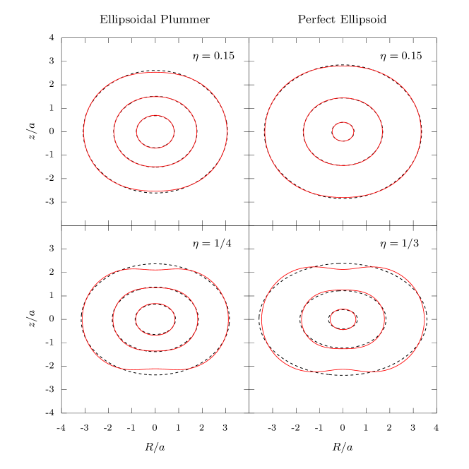
Figure 1: Isodensity contours, normalised to $\rho_{\rm n}$, for the P11 (left) and ZL85 (right) models. Dashed lines refer to the ellipsoidal (original) model, while solid red lines to the $\eta$-linear expansion of the density, as given in equation (13). Contours correspond to values of $1$, $10^{-1}$, and $10^{-2}$ from inside to outside. The bottom panels show the case of the critical flattenings $\eta=1/4$ for P11 models, and $\eta=1/3$ for ZL85 ones: for larger values of $\eta$ the truncated density in equation (13) would be negative near the $z$-axis (see equation 12). The outermost expanded contours differ most from the elliptical shape as $\eta$ increases.

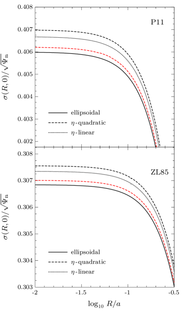
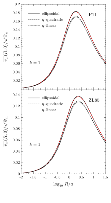
Figure 2: Left: radial profile of the velocity dispersion $\sigma$ in the equatorial plane ($z=0$) for the models discussed in Section 4, with $\eta=0.1$, and without a central BH ($\mu=0$). The homoeoidal approximation reproduces remarkably well the full solution (solid line), over the displayed radial range of $0.01<R/a\lesssim 0.32$. The values of $\sigma$ for the $\eta$-linear models overestimate the full solution, and retaining the quadratic terms in the flattening further increases this overestimate. Right: radial trend of $\overline{\varv_{\varphi}}$ on the equatorial plane, for the same models on the left, and with the same meaning of the line-type; the case of the isotropic rotator is shown. The values of $\overline{\varv_{\varphi}}$ for the $\eta$-linear and $\eta$-quadratic models underestimate those of the full solution. In all panels, the red dashed line shows the expansion up to the quadratic order in $\eta$ of the full solution (see equation 40, and Section 4.1).

3.3 The $\eta$-quadratic solution of the Jeans equations

In this Section we present the general $\eta$-quadratic solution for the homoeoidal expansion of a model with a central BH of mass $M_{\rm{BH}}=\mu M$; quite obviously, the $\eta$-linear solution is just obtained by ignoring the quadratic terms. As usual, we split the velocity dispersion into the contribution $\sigma_{*}$, due to the potential of the model for the stellar component, and $\sigma_{\rm BH}$, the one due to the potential of the BH: $\sigma^{2}=\sigma_{*}^{2}+\sigma_{\rm BH}^{2}$. By inserting the expansions (13) in equation (18), with $\Psi_{\rm T}$ given by equation (16), some algebra shows that

$$\frac{\rho\hskip 0.42677pt\sigma_{*}^{2}}{\rho_{\rm n}\Psi_{\rm n}}= \frac{H_{00}(s)}{2}+\eta\hskip 0.56905pt\big{[}\hskip 0.42677ptH_{01}(s)+\tilde{R}^{2}H_{02}(s)\hskip 0.28453pt\big{]}$$ (21)

$$+\eta^{2}\left[\hskip 0.56905pt\frac{H_{11}(s)}{2}+\tilde{R}^{2}H_{12}(s)+\tilde{R}^{4}\hskip 0.56905pt\frac{H_{22}(s)}{2}\hskip 0.28453pt\right],$$

and

$$\frac{\rho\hskip 0.42677pt\sigma_{\rm BH}^{2}}{\rho_{\rm n}\Psi_{\rm n}}=\mu\hskip 0.28453pt\big{[}\hskip 0.28453ptY_{0}(s)+\eta\hskip 0.56905ptY_{1}(s)+\eta\hskip 0.56905pt\tilde{R}^{2}Y_{2}(s)\hskip 0.28453pt\big{]}\hskip 0.56905pt,$$ (22)

where, for $i,j=0,1,2$, the dimensionless functions $H_{ij}(s)\equiv X_{ij}(s)+X_{ji}(s)$ and $Y_{i}(s)$ are given by

$$X_{ij}(s)\equiv-\int_{s}^{\infty}\rho_{i}(t)\hskip 0.56905pt\frac{d\Psi_{j}(t)}{dt}\hskip 0.7113ptdt\hskip 0.56905pt,\qquad Y_{i}(s)\equiv\int_{s}^{\infty}\frac{\rho_{i}(t)}{t^{2}}\hskip 0.56905ptdt\hskip 0.56905pt,$$ (23)

and $\rho_{i}$ and $\Psi_{i}$ are given in equation (14); notice that $H_{ij}=H_{ji}$.

We then evaluate $\Delta=\Delta_{*}+\Delta_{\rm BH}$ from equation (19), where $\Delta_{*}$ and $\Delta_{\rm BH}$ are the contributions due to the potential of the stars and the one due to the potential of the central BH, respectively. From equations (19), (13), and (20), we obtain

$$\frac{\rho\hskip 0.42677pt\Delta_{*}}{\rho_{\rm n}\Psi_{\rm n}}=2\hskip 1.13809pt\eta\hskip 0.56905pt\tilde{R}^{2}\big{[}Z_{02}(s)+\eta\hskip 0.56905ptZ_{12}(s)+\eta\hskip 0.56905pt\tilde{R}^{2}Z_{22}(s)\big{]},$$ (24)

and

$$\frac{\rho\hskip 0.42677pt\Delta_{\rm BH}}{\rho_{\rm n}\Psi_{\rm n}}=2\hskip 0.56905pt\mu\hskip 0.85358pt\eta\tilde{R}^{2}Y_{2}(s)\hskip 1.13809pt,$$ (25)

where $Z_{ij}(s)\equiv H_{ij}(s)-\rho_{i}(s)\hskip 0.56905pt\Psi_{j}(s)$. As expected, $\Delta_{*}$ and $\Delta_{\rm BH}$ vanish for $\eta=0$; moreover, $\sigma_{\rm BH}^{2}$ and $\Delta_{\rm BH}$ depend linearly on $\eta$ also in the $\eta$-quadratic interpretation.

A comment is in order here, about the fact that in the $\eta$-linear and $\eta$-quadratic frameworks the expressions above refer to the products $\rho\hskip 0.42677pt\sigma^{2}$ and $\rho\hskip 0.42677pt\Delta$, and not to the purely kinematical fields $\sigma^{2}$ and $\Delta$. In order to obtain $\sigma^{2}$ and $\Delta$, one must divide $\rho\hskip 0.42677pt\sigma^{2}$ and $\rho\hskip 0.42677pt\Delta$ by the density in equation (13), i.e., by a linear function in $\eta$. In the $\eta$-linear case one should then expand the fraction up to linear terms in $\eta$; in the $\eta$-quadratic interpretation, instead, where the density-potential pair in equation (13) is considered a model by itself, one should not expand, so that the purely kinematical fields are not polynomial functions of the flattening. Of course, in the limit of small flattening, even in the $\eta$-quadratic interpretation, the kinematical fields can be expanded up to $\eta^{2}$ terms included, thus obtaining more manageable expressions.

4 The Models

We now consider axisymmetric systems of density distribution $\rho(R,z)$, total mass $M$, scale length $a$, and axial ratio $q=1-\eta$, where $0\leq\eta<1$. From equations (1) and (2) with $\epsilon=0$, one has:

$$\frac{\rho(R,z)}{\rho_{\rm n}}=\frac{\tilde{\rho}(m)}{1-\eta}\hskip 0.56905pt,\qquad m^{2}=\tilde{R}^{2}+\hskip 0.56905pt\frac{\tilde{z}^{2}}{(1-\eta)^{2}}\hskip 0.56905pt.$$ (26)

In particular, we solve in closed form the $\eta$-quadratic Jeans equations for two ellipsoidal models: the ellipsoidal generalization of the Plummer model (P11), and the Perfect Ellipsoid (ZL85). The $\eta$-linear cases are immediately obtained by neglecting the $\eta^{2}$ terms. The dimensionless densities of the two models are given respectively by

$$\tilde{\rho}(m)=\ \begin{dcases}\hskip 1.42271pt\frac{3}{(1+m^{2})^{5/2}}\hskip 0.28453pt,\\[4.0pt] \hskip 1.42271pt\frac{4}{\pi\hskip 0.28453pt(1+m^{2})^{2}}\hskip 0.28453pt,\end{dcases}$$ (27)

and the masses enclosed within $m$ are

$$\frac{M(m)}{M}=\begin{dcases}\hskip 1.42271pt\frac{m^{3}}{(1+m^{2})^{3/2}}\hskip 0.28453pt,\\[4.0pt] \hskip 1.42271pt\frac{2}{\pi}\left(\hskip 0.85358pt\arctan m-\frac{m}{1+m^{2}}\hskip 0.56905pt\right).\end{dcases}$$ (28)

In the adopted notation, the circular velocity in the equatorial plane can be written as

$$\frac{\varv_{\rm c}^{2}(R\hskip 0.42677pt)}{\Psi_{\rm n}}=\frac{\tilde{R}^{2}}{2}\bigintsss_{\hskip 1.13809pt0}^{\infty}\tilde{\rho}\left(\frac{\tilde{R}}{\sqrt{1+u\hskip 1.13809pt}}\right)\frac{du}{(1+u)^{2}\sqrt{\hskip 0.28453ptq^{2}+u\hskip 1.13809pt}}\hskip 0.56905pt,$$ (29)

(e.g., see equation 5.62 in C21), and for P11 we obtain

$$\frac{\varv_{\rm c}^{2}(R\hskip 0.42677pt)}{\Psi_{\rm n}}=\frac{p^{2}\hskip 0.56905pt\mathbb{F}\hskip 0.85358pt(\phi,k)+(\tilde{R}^{2}-p^{2})\hskip 0.85358pt\mathbb{E}\hskip 0.85358pt(\phi,k)}{(p^{2}+\tilde{R}^{2})^{3/2}}-\frac{q\hskip 0.28453pt\tilde{R}^{2}}{(p^{2}+\tilde{R}^{2})(1+\tilde{R}^{2})^{3/2}}\hskip 0.28453pt,$$ (30)

where

$$\phi\equiv\arcsin\sqrt{\hskip 0.7113pt\frac{p^{2}+\tilde{R}^{2}}{1+\tilde{R}^{2}}\hskip 0.28453pt}\hskip 0.85358pt,\quad k\equiv\frac{\tilde{R}}{\sqrt{p^{2}+\tilde{R}^{2}}}\hskip 0.7113pt,\quad p^{2}\equiv 1-q^{2},$$ (31)

and $\mathbb{F}\hskip 0.85358pt(\phi,k)$ and $\mathbb{E}\hskip 0.85358pt(\phi,k)$ are the Legendre elliptic integrals of first and second kind in trigonometric form (e.g. Gradshteyn & Ryzhik 2007). For ZL85 we have:

$$\frac{\varv_{\rm c}^{2}(R\hskip 0.42677pt)}{\Psi_{\rm n}}=\frac{2\tilde{R}^{2}}{\pi\hskip 0.28453pt(p^{2}+\tilde{R}^{2})}\left(\hskip 0.28453pt\frac{\phi}{\sqrt{p^{2}+\tilde{R}^{2}}}-\frac{q}{1+\tilde{R}^{2}}\hskip 0.28453pt\right),$$ (32)

where $p$ and $\phi$ are given in equation (31). Equations (30) and (32) are exact for any finite value of $\eta$; with some work, they can be expanded to any desired order in $\eta$, thus providing a check for the homoeoidal expansion, where

$$\frac{\varv_{\rm c}^{2}(R\hskip 0.42677pt)}{\Psi_{\rm n}}=\varv^{2}_{0}(\tilde{R}\hskip 0.56905pt)+\eta\hskip 0.56905pt\varv^{2}_{1}(\tilde{R}\hskip 0.56905pt)\hskip 0.56905pt,\qquad\varv_{i}^{2}(\tilde{R}\hskip 0.56905pt)\equiv-\hskip 1.13809pt\tilde{R}\hskip 1.42262pt\frac{d\psi_{i}(\tilde{R}\hskip 0.56905pt)}{d\tilde{R}}\hskip 0.56905pt.$$ (33)

We verified that the linear expansion of equations (30) and (32) are in perfect agreement with equation (33), where $\varv_{0}$ and $\varv_{1}$ are given in the Appendix.

For an axisymmetric model with a central BH, the full solution of equations (18) and (19) can be recast in integral form by exploiting the assumed homoeoidal structure. For the contributions of the stellar-dynamical models we have

$$\frac{\rho\hskip 0.42677pt\sigma_{*}^{2}}{\rho_{\rm n}\Psi_{\rm n}}=\frac{1}{2q}\bigintsss_{\hskip 1.13809pt\tilde{z}}^{\infty}\tilde{\rho}(m^{\prime})\hskip 0.85358pt\tilde{z}^{\prime}d\tilde{z}^{\prime}\bigintsss_{\hskip 1.13809pt0}^{\infty}\frac{\tilde{\rho}(m_{u})\hskip 0.56905ptdu}{(1+u)(q^{2}+u)^{3/2}}\hskip 0.56905pt,$$ (34)

and

$$\frac{\rho\hskip 0.42677pt\Delta_{*}}{\rho_{\rm n}\Psi_{\rm n}}=\frac{p^{2}\tilde{R}^{2}}{2q^{3}}\bigintsss_{\hskip 1.13809pt\tilde{z}}^{\infty}\hskip 1.13809pt\left|\frac{d\tilde{\rho}(m^{\prime})}{dm^{\prime}}\hskip 0.28453pt\right|\frac{\tilde{z}^{\prime}d\tilde{z}^{\prime}}{m^{\prime}}\bigintsss_{\hskip 1.13809pt0}^{\infty}\frac{\tilde{\rho}(m_{u})\hskip 0.56905ptu\hskip 0.28453ptdu}{(1+u)^{2}(q^{2}+u)^{3/2}},$$ (35)

where $p^{2}=1-q^{2}$, $m_{u}=m({\bf x},u)$ is given by equation (6), $m^{\prime}=\sqrt{\tilde{R}^{2}+\tilde{z}^{\prime 2}/q^{2}}$, and the two integrals are evaluated at fixed $\tilde{R}$ (e.g., see exercise 13.29 in C21). The contributions due to a central BH of mass $M_{\rm{BH}}=\mu M$ are instead given by

$$\frac{\rho\hskip 0.42677pt\sigma_{\rm BH}^{2}}{\rho_{\rm n}\Psi_{\rm n}}=\frac{\mu}{q}\bigintsss_{\hskip 1.13809pt\tilde{z}}^{\infty}\tilde{\rho}(m^{\prime})\hskip 0.7113pt\frac{\tilde{z}^{\prime}d\tilde{z}^{\prime}}{s^{\prime\hskip 0.42677pt3}},$$ (36)

and

$$\frac{\rho\hskip 0.42677pt\Delta_{\rm BH}}{\rho_{\rm n}\Psi_{\rm n}}=\frac{\mu\hskip 0.28453ptp^{2}\tilde{R}^{2}}{q^{3}}\bigintsss_{\hskip 1.13809pt\tilde{z}}^{\infty}\hskip 1.13809pt\left|\frac{d\tilde{\rho}(m^{\prime})}{dm^{\prime}}\hskip 0.28453pt\right|\frac{\tilde{z}^{\prime}d\tilde{z}^{\prime}}{m\hskip 0.7113pts^{\prime\hskip 0.42677pt3}},$$ (37)

where $s^{\prime}=\sqrt{\tilde{R}^{2}+\tilde{z}^{\prime 2}}$ (e.g., see exercise 13.28 in C21).

Finally, for what concerns the self-gravitational energy of the models, the integral in equation (7) evaluates to $3\pi/4$ and $4/\pi$, respectively for the P11 models and ZL85 models, so that, by expanding up to the second order in $\eta$ the coefficients $\varw_{i}$ in equation (7), for the axisymmetric case one has

$$\frac{W}{M\Psi_{\rm n}}\sim-\hskip 1.13809pt\frac{1}{8}\left(1+\frac{\eta}{3}+\frac{2\hskip 0.56905pt\eta^{2}}{15}\right)\int_{0}^{\infty}F^{2}(m)\hskip 0.56905ptdm\hskip 0.28453pt.$$ (38)

This expression can be used as a check of the homoeoidal expansion, when the self-gravitational energy is computed directly from the density-potential pair in equation (13), limiting to the linear terms in $\eta$.

Figure 3: The $\eta$-linear modelling of an isotropic ($k=1$) system with $\eta=0.1$, and a central BH with $\mu=0.001$, for the models in Section 4. Solid lines show $\sigma$ (left) and $\overline{\varv_{\varphi}}$ (right) on the equatorial plane ($z=0$). Dotted and dashed lines show respectively the contributions of the stellar-dynamical model and the BH. Due to the presence of the BH, the velocity dispersion diverges at small radii as $1/\sqrt{R}$, while the streaming velocity vanishes towards the center as $\sqrt{R}$ (see Section 4.1).

4.1 Results

As recalled in Section 2, in the homoeoidal expansion there is an upper limit on $\eta$ (that depends on the truncation order), so that, for $\eta$ smaller than the critical value, the truncated density is nowhere negative: from (12), $\eta\leq 1/4$ for P11 models, and $\eta\leq 1/3$ for ZL85 models. Reassuringly, these critical values are quite large, allowing to deal with moderately flattened stellar systems such as those discussed in Section 5. In general, for $\eta$ close to the limit, the density tends to become negative along the $z$-axis, producing densities with a ‘torus-like’ structure, similar to the Binney logarithmic halo for potential flattening near the critical value (BT08), and to complex shifted models (e.g. Ciotti & Giampieri 2007). In Fig. 1 we show the isodensity contours of P11 and ZL85 models, for two different $\eta$ values. Black dashed lines show the original ellipsoidal models in equation (27), while red solid lines show the homoeoidally expanded models in equation (13), where the explicit expressions for $\rho_{i}$ are given in Appendix. The figure shows how well the truncated density reproduces the original model with $\eta=0.15$, and how a toroidal shape in the outer parts of the systems appears for $\eta$ approaching the critical value. Of course, truncating the density up to the quadratic order in $\eta$ increases the upper limit on the flattening, and both black and red isdodensities would be almost indistinguishable also in the analogous of Fig. 1 (not shown here for simplicity).

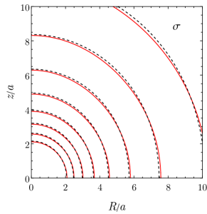
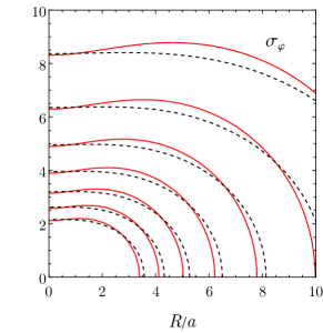
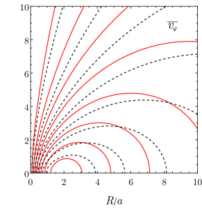
Figure 4: Maps of $\sigma$ (left), $\sigma_{\varphi}$ (middle, $k=0$), and $\overline{\varv_{\varphi}}$ (right, $k=1$), in units of $\sqrt{\Psi_{\rm n}}$, for P11 models with $\eta=0.1$ and $\mu=0$. Dashed lines show the full solution, solid red lines show the solution of the $\eta$-linear modelling. The innermost contour corresponds to values of $0.26$ for the normalized $\sigma$ and $\sigma_{\varphi}$, and of $0.16$ for $\overline{\varv_{\varphi}}$. The values for the other contour lines decrease outward with steps of $0.02$.

In order to address the first goal of this work, i.e., to evaluate how $\eta$-linear and $\eta$-quadratic solutions compare between them and with respect to the full solutions for genuine ellipsoidal models, in Fig. 2 we show the velocity dispersion $\sigma$, and the streaming velocity $\overline{\varv_{\varphi}}$ in the equatorial plane, for P11 and ZL85 models for a flattening $\eta=0.1$, and in the isotropic rotator ($k=1$). The solutions are shown in absence of the central BH for simplicity; the explicit expressions for the functions $X_{i}$, $Y_{i}$, $H_{ij}$ and $Z_{ij}$, entering $\rho\hskip 0.42677pt\sigma_{*}^{2}$ and $\rho\hskip 0.42677pt\Delta_{*}$ in equations (21) and (24), are given in the Appendix. We first focus on $\sigma$. For each model, the left panels of Fig. 2 show the full solution for the ellipsoidal model (black solid line), obtained by solving numerically equation (34), the $\eta$-linear solution (dotted line), the $\eta$-quadratic solution (dashed line), and the truncated expansion of the full solution up to the quadratic order terms included (red dashed line). For reference, the central values of $\sigma$ in the $\eta$-quadratic solutions are

$$\frac{\sigma_{0}^{2}}{\Psi_{\rm n}}=\begin{cases}\displaystyle\frac{2+4(67-96\ln 2)\hskip 0.56905pt\eta+3(355-512\ln 2)\hskip 0.56905pt\eta^{2}}{12(1+\eta)}\hskip 0.56905pt,\\[14.0pt] \displaystyle\frac{3(32-3\pi^{2})+8(9\pi^{2}-88)\hskip 0.56905pt\eta+24(15\pi^{2}-148)\hskip 0.56905pt\eta^{2}}{24\pi(1+\eta)}\hskip 0.56905pt,\end{cases}$$ (39)

for the P11 and ZL85 models respectively. Obviously, the $\eta$-linear case is obtained by neglecting the $\eta^{2}$ terms at the numerators. A few general features are apparent. The first is the expected similarity of the full solution for the two models, due to the qualitatively similar behaviour of their density distributions in the central regions. In the external regions, the decline of $\sigma$ in both models goes as $R^{-1/2}$ being $\rho\hskip 0.42677pt\sigma_{*}^{2}\propto r^{-\hskip 0.85358pt6}$ for the P11 models, and $\rho\hskip 0.42677pt\sigma_{*}^{2}\propto r^{-\hskip 0.85358pt5}$ for the ZL85 ones.

The second reassuring feature is how close the full solution and those in the homoeoidal approximation are, over the whole radial range: the percentual differences are so small (less than $0.3\%$) to be completely negligible in all practical applications. Therefore, we can conclude that the effect of quadratic $\eta$ terms is negligible, and that the $\eta$-linear approximation, with its simplifications, can be safely used to model systems with low flattening.

We can now address an interesting result that emerges from Fig. 2, also completing the reasonings introduced at the end of Section 3.3. For both models, the $\eta$-linear solution always overestimates the full solution (with differences decreasing for increasing $R$), and so do the other approximations; however, the $\eta$-quadratic solutions differ from the full solution more than the $\eta$-linear solutions. This result might be unexpected, since a quadratic approximation should perform better than a linear one. But it should be recalled that the $\eta$-quadratic solution is not the quadratic approximation of the full solution. In fact, the dashed red lines in Fig. 2 confirm that the quadratic approximation $(\rho\hskip 0.42677pt\sigma_{*}^{2})_{\rm quadratic}$ performs better than the $\eta$-linear solution $(\rho\hskip 0.42677pt\sigma_{*}^{2})_{\eta-{\rm linear}}$. As discussed in Section 3.3, the quadratic expansion of the full solution

$$(\rho\hskip 0.42677pt\sigma_{*}^{2})_{\rm quadratic}\simeq(\rho\hskip 0.42677pt\sigma_{*}^{2})_{\rm\eta-{\rm linear}}+\eta^{2}Q$$ (40)

could be computed formally starting from the homoeoidal truncation of the density-potential pair to the quadratic order in $\eta$, solving the Jeans equations, and finally discarding all terms in flattening of order higher than quadratic. However, instead of performing such laborious mathematical calculations, we computed numerically the function $Q$ in equation (40) as

$$Q\equiv\lim_{\eta\to 0}\frac{\rho\hskip 0.42677pt\sigma_{*}^{2}-(\rho\hskip 0.42677pt\sigma_{*}^{2})_{\rm\eta-{\rm linear}}}{\eta^{2}}\hskip 0.56905pt,$$ (41)

where $\rho\hskip 0.42677pt\sigma_{*}^{2}$ is the full (numerical) solution. In the formula above, the numerical value of $\eta$ are reduced until convergence is reached (but maintained large enough to avoid numerical fluctuations). The fact that the $\eta$-quadratic solution is not the quadratic truncation of the expansion of the full solution is made apparent by the fact that the black dashed lines (the $\eta$-quadratic solutions) are more distant from the solid line than the $\eta$-linear solution (dotted lines); this is due to the missing quadratic terms, which can be shown to be collectively negative. The conclusion is that, when using the homoeoidal expansion to describe an ellipsoidal system, the $\eta$-linear interpretation is to be preferred to the $\eta$-quadratic solution, not only for its greater simplicity, but also for its better accuracy.

The right panels of Fig. 2 show the corresponding streaming velocity profile $\overline{\varv_{\varphi}}$ in the equatorial plane for the isotropic case ($k=1$); the radial range has been extended to $R\simeq 32\hskip 1.13809pta$, in order to display the whole peak present at around $R\simeq 1.6\hskip 1.13809pta$. The Satoh decomposition can be adopted for these models given the positivity of $\Delta_{*}$, which is to be expected since $\Delta$ is nowhere negative for an oblate self-gravitating ellipsoid, as shown by equation (35). Several of the comments concerning the solutions for the velocity dispersion apply also to $\overline{\varv_{\varphi}}$, in particular that on the almost perfect (for practical purposes) coincidence of the $\eta$-linear, $\eta$-quadratic, and full solutions. However, the $\eta$-linear solutions are now the most discrepant with respect to the full solutions, followed, in order, by the $\eta$-quadratic and the true quadratic expansion.

The effect of a central BH of mass $M_{\rm{BH}}=10^{-3}M_{*}$ on the $\eta$-linear solution is shown for the P11 and ZL85 models in Fig. 3. In each plot, the solid line is the total, the dashed line is the BH contribution, and the dotted line is the model for the stellar component already shown in Figure 2; the radial range is now extended down to $R=10^{-3}\hskip 0.56905pta$ to better appreciate the dynamical effects of the BH. From equation (28), the radius contaning the fraction $\mu=10^{-3}$ of the total mass (of the spherical model), that is the commonly adopted estimate for the dynamical radius of the BH (see Chapter 4 in BT08), is $R_{\rm dyn}\approx 0.1\hskip 0.56905pta$. This value is nicely close to the position where the lines corresponding to the total $\sigma$ and $\overline{\varv_{\varphi}}$ start to deviate from the stellar-dynamical model contributions. In particular, the BH determines an increase of $\sigma$ towards the centre that goes as $R^{\hskip 0.56905pt-1/2}$; instead, $\overline{\varv_{\varphi}}$ still vanishes at the centre even in the presence of the BH. This property can be quantified with the asymptotic analysis of $\Delta_{*}$ and $\Delta_{\rm BH}$ near the center: without the BH, the isotropic $\overline{\varv_{\varphi}}$ decreases at small radii as $R$, whereas in presence of the BH it decreases as $R^{\hskip 0.56905pt1/2}$; thus, $\overline{\varv_{\varphi}}$ does not diverge at the centre, as instead $\sigma$ and $\varv_{\rm c}$ do. This is explained by noticing that, for a generic model density with a central profile $(1+m^{2})^{-\alpha}$, $\Delta_{\rm BH}\propto R^{2}/r$ at small radii, and so in the Satoh decomposition $\overline{\varv_{\varphi}}$ vanishes towards the centre, while $\overline{\varv_{\varphi}^{2}}$ diverges as $\sigma^{2}$. Of course, when adopting a different decomposition of $\overline{\varv_{\varphi}^{2}}$ (such as that in equation 13.107 in C21; see also De Deo et al. 2024), a central cusp in $\overline{\varv_{\varphi}}$ would be obtained. We conclude that special care should be used when interpreting the results of models used to predict the effects of a central BH on the streaming velocity field of the stars.

The previous discussion focused on the different solutions on the equatorial plane. It is of course important to consider also their behavior over the full $(R,z)$ plane, as 2D spectroscopy is nowadays routinely performed (e.g. Emsellem et al. 2007; Krajnović et al. 2008; Jeong et al. 2009). In Fig. 4 we show the two-dimensional maps of $\sigma$, $\sigma_{\varphi}$, and $\overline{\varv_{\varphi}}$ (for $k=1$), for a P11 model with $\eta=0.1$ and $\mu=0$; contours are displayed for the full and the $\eta$-linear solutions. The comparison shows that the $\eta$-linear $\sigma$ keeps extremely close to that of the full solution, even outside the equatorial plane; a similar agreement persists for $\sigma_{\varphi}$, while it becomes slightly worse for $\overline{\varv_{\varphi}}$. However, even if the shape of the isorotational surfaces in the $\eta$-linear approximation seems more discrepant from that of the true solution than for the $\sigma$ and $\sigma_{\varphi}$ cases, the $\overline{\varv_{\varphi}}$ values of the $\eta$-linear and full solutions along cuts at fixed $z$ are still very similar, as we verified with plots of these cuts (where indeed the differences in velocity are of the same extent as in the left panels of Fig. 2).

5 An application: rotation and flattening of globular clusters

Globular Clusters (GCs) have traditionally been regarded as simple spherical, non-rotating stellar systems; however, small ellipticities have been observed since a long ago, and rotation is being detected in a growing number of them (e.g., Bianchini et al. 2018, Kamann et al. 2018, Ferraro et al. 2018). The origin of the observed flattening has been attributed to the effects of internal rotation, velocity dispersion anisotropy, and external tides (for a more extended discussion, see e.g. van den Bergh 2008). In particular, dynamical phenomena such as violent relaxation and two-body relaxation tend to produce isotropic velocity distributions in the central regions of stellar systems, so that, if flattening is observed there, rotation should be considered a possible explanation. In addition to contributing to the shape of these systems, rotation is also expected to change their dynamical evolution (e.g., Fiestas et al. 2006), and to be linked to their ‘dynamical age’ (e.g., Tiongco et al. 2017; Livernois et al. 2022, Leanza et al. 2022). Finally, rotation has been suggested to have a role in the formation of multiple stellar populations in them (Lacchin et al. 2023). Therefore, an assessment of the respective amounts of rotation and anisotropic pressure is particularly important. Indeed, in recent years much effort has been devoted to dynamical modelling of GCs, using different strategies, as for example $N$-body simulations (e.g., Hurley & Shara 2012), Monte Carlo models (e.g., Giersz et al. 2013; Kamlah et al. 2022), or self-consistent models specific for quasi-relaxed, rotating stellar systems (Varri & Bertin 2012, Bianchini et al. 2013, Jeffreson et al. 2017); see Spurzem & Kamlah (2023) for a recent review.

In general, these techniques are quite complex, and their application time-consuming: it would be desirable to have a simple but robust method to assess phenomenologically the importance of rotation, before applying more sophisticated tools, and we suggest that the homoeoidal expansion and the $\eta$-linear solutions of the Jeans equations could be one of such possibilities. Moreover, for the choice of Satoh’s decomposition and for a density profile roughly constant in the central regions, the homoeoidal expansion predicts a sort of ‘universal profile’ for the streaming velocity $\overline{\varv_{\varphi}}$, of shape given by the first of equation (17) with $k=1$, coupled to equations (24) and (25). In particular, three main properties are predicted: (1) from equation (24), $\overline{\varv_{\varphi}}$ scales as the square root of flattening, and increases linearly with radius; (2) it reaches a maximum; (3) it decreases afterward. Of course these properties transfer also to the projected streaming velocity field $\varv_{\rm los}$. Thus, a simple and direct relation between the shape of the system and its rotation profile is expected, and it is tempting here to test whether it is satisfied by well observed systems. At first sight, the three features of $\overline{\varv_{\varphi}}$ (and $\varv_{\rm los}$) agree with what observed, for a chosen test-case object (see below), and also for others (e.g., Leanza et al. 2022). Therefore, the method could provide a fast and flexible tool to address, in a preliminary way, the following questions: are observations consistent with velocity dispersion isotropy? if not, does a rescaling of $\varv_{\rm los}$ with a different costant $k$ value make the model consistent with observations? or, is there the need for a change of $k$ with radius?

As a test-case for the application of the homoeoidal method we chose NGC 4372, a GC for which a detailed photometric and spectroscopic study was conducted (Kacharov et al. 2014). NGC 4372 has an observed low ellipticity of $\eta=0.08$; and, thanks to a large number of precise radial velocity measurements, it has a $\varv_{\rm los}$ profile extending at least out to its half-light radius, and a velocity dispersion profile extending even further out. Kacharov et al. (2014) adopted a Plummer model, one of the two illustrating cases above, as an optimal representation of the observed properties; they estimated $a=5.1\,{\rm pc}$, and $M=1.7\times 10^{5}\,M_{\odot}$. All this makes NGC 4372 an obvious candidate for our test. We modelled then NGC 4372 with the P11 profile, of parameters as in Kacharov et al., and, based on the results of Section 4.1, with the $\eta$-linear solution of the Jeans equations. For the model, and for $k=1$, Figure 5 shows the intrinsic streaming velocity $\overline{\varv_{\varphi}}$ (blue solid curves), the line-of-sight velocity $\varv_{\rm los}$ (blue dashed curves), and the line-of-sight velocity dispersion $\sigma_{\rm los}$ (see Section 5 in CMPZ21 and Chapter 11 in C21 for the formulae used to obtain the projected quantities); the corresponding observed data points (red dots) are also shown for comparison, together with the their error bars. When projecting, we adopted two inclination angles: $i=90^{\circ}$ (upper panels in Fig. 5) and $i=45^{\circ}$ (lower panels). In the first case, NGC 4372 is supposed to be viewed edge-on, and the model was built with an intrinsic flattening coincident with the observed one ($\eta=0.08$); in the second case, the intrinsic flattening increases to $\eta=0.17$. Overall, for both inclinations, $\sigma_{\rm los}$ of the model accounts quite well for the observed profile, but the isotropic $\varv_{\rm los}$ does not so: its innermost rising part does not reproduce well the observed curve, and, more important, at distances larger than $\simeq a$ it remains too high. We are then forced to exclude the possibility that NGC 4372 is an isotropic rotator, and also that it is a rotator with a different but constant $k$, that would have a $\varv_{\rm los}$ profile with the same shape, just rescaled. Notice that decreasing further the inclination angle would not change significantly this conclusion: it would produce an increased intrinsic flattening, and then an increase of the isotropic $\overline{\varv_{\varphi}}$, that would be almost perfectly compensated by the decrease of the projection angle.

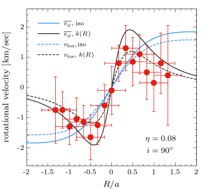
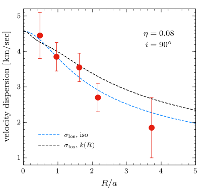
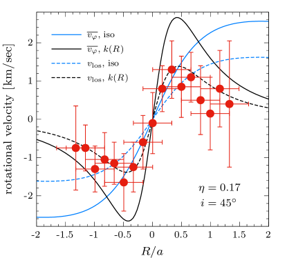
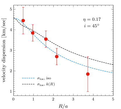
Figure 5: The $\eta$-linear modelling of the Globular Cluster NGC 4372, whose observed (projected along the line-of-sight) kinematics is shown by red points (from Kacharov et al. 2014). Solid lines show the intrinsic velocity $\overline{\varv_{\varphi}}$; dashed lines show the projected velocity $\varv_{\rm los}$ (on the left) and $\sigma_{\rm los}$ (on the right). Blue lines show the isotropic case ($k=1$), black lines the spatially-dependent $k(R\hskip 0.56905pt)$ in equation (42). Two inclination angles were adopted: $i=90^{\circ}$ (upper panels) and $i=45^{\circ}$ (lower panels). When $i=90^{\circ}$, the intrinsic flattening coincides with the observed one ($\eta=0.08$); when $i=45^{\circ}$, the intrinsic flattening is $\eta=0.17$ (see Section 5).

Having discarded the possibility of an isotropic rotator, we attempted then to reproduce the observed profile with a radially dependent Satoh decomposition. Since the blue solid curves in Fig. 5 give the $\overline{\varv_{\varphi}}$ field with $k=1$ in equation (17), in practice they also show $\sqrt{\Delta}$ and its projection; the modifications needed on $k$ can be then easily deduced from these curves. Quite obviously, we do not attach a deep physical meaning to these modifications, even though some implications can be derived. An inspection of Fig. 5 suggests that the required changes to $\varv_{\rm los}$, to be produced by a radially dependent $k$, are: (i) preserve the linear rise of $\varv_{\rm los}$ in the central regions, but include a sharp peak at a radius of $\sim a/3$, that is not present in the constant $k$ case; (ii) be significantly lower than the isotropic rotation velocity outside $\simeq a$. We parametrized these requests with the trial function

$$k(R\hskip 0.56905pt)=\frac{A}{1+(\tilde{R}/B)^{n}},$$ (42)

where $\tilde{R}=R/a$, and $A$, $B$ and $n$ are three dimensionless free parameters. In Fig. 5 with black lines we show the intrinsic and projected streaming velocity profiles, obtained from equation (42), with $A=3.5$, $B=0.5$, and $n=2$, and for the two inclination angles $i=90^{\circ}$ and $i=45^{\circ}$. The chosen values of $A$, $B$ and $n$ are not the result of a rigorous “best fitting” procedure; they reproduce quite reasonably the observed velocity profile, and allow us to draw three robust conclusions: the central regions must rotate faster than the isotropic rotator, as $k\simeq 3.5$ there; rotation is very concentrated; and the $\overline{\varv_{\varphi}}$ decline for $R\gtrsim a/2$ is steep, with $k\propto 1/R^{2}$. The lack of proper motion measurements for NGC 4372 prevented us from establishing the inclination angle, thus the intrinsic flattening. It would be interesting to extend our analysis to some other GCs with well-measured proper motions; however, as stressed above, we found a compensation between the system inclination and $\varv_{\rm los}$, therefore we are confident that the results obtained are quite robust.

The right panels of Fig. 5 also show that, with the $k(R)$ in equation (42), $\sigma_{\rm los}$ differs from that of the isotropic rotator, which is not a surprise because $\varv_{\rm los}$ enters the expression for $\sigma_{\rm los}$ (see e.g. equation 54 in CMPZ21): this is at the origin of the (small) drop of the black lines in the very central regions. In particular, the two outermost data points are better reproduced by the isotropic $\sigma_{\rm los}$ rather than the new one. We believe that a formal solution, reproducing both $\varv_{\rm los}$ and $\sigma_{\rm los}$, could be obtained by using a more complicated functional form of $k(R)$, for example that increases again up to unity outer of the most external observed point of $\varv_{\rm los}$; however, we consider this possibility quite implausible from a physical point of view. We conclude that NGC 4372 is unlikely to be an isotropic rotator, because of its lower rotation at $R\gtrsim a$, and a higher rotation in its central region. Reassuringly, some of these conclusions have been also reached with a more sophisticated approach, based on the construction of models supported by a self-consistent phase-space distribution function (e.g. Varri & Bertin 2012, Jeffreson et al. 2017).

Before concluding this analysis, it is tempting to suggest another possible interpretation for the observed kinematic features of NGC 4372: the GC could be a two-component system, with an inner rotating structure physically distinct from that of the main body of the GC, and described by its own phase-space distribution function. Our modelling so far was implicitly based on the use of a single distribution function, i.e., the GC was assumed to be a one-component system. If the total distribution function were the sum of two different distribution functions, one for the non-rotating (or slowly rotating) GC, and the other for the fast rotating substructure, the total rotational field to be modelled with the Jeans equations were the mass averaged rotational field of the GC and of the substructure (not just that of the sampled stars of the subcomponent). It would be interesting to determine observationally if the stars contributing to the projected streaming velocity in the central region show a difference in age and/or chemical composition with respect to the majority of the stars of the GC.

A different possibility would be that the rotational profile is explained by a significant change in the flattening of the system approaching the centre; in fact the ellipticity is observed to vary in the central regions of some GC (e.g. Bianchini et al. 2013). The possibility that the inner regions can be actually interpreted as a flattened isotropic rotator is qualitatively supported by the scaling of the isotropic $\overline{\varv_{\varphi}}$ with $\sqrt{\eta}$. We note however that in NGC 4372 the fiducial value $\simeq 3$ of the Satoh $k$ parameter in the central regions would require, if decreased to 1, an increase of the adopted $\eta$ by a factor of $\approx 9$, bringing the flattening well above the limiting value allowed by the homoeoidal expansion.

6 Discussion and conclusions

In this work we studied some aspects of the Jeans modelling of axisymmetric systems that are only slightly deviating from a spherical shape, a situation often encountered in applications. In particular, we considered two problems related to the homoeoidal expansion technique (CB05; CMPZ21; C21; see also Lee and Suto 2003; Muccione and Ciotti 2004; Ciotti et al. 2006; Ciotti and Pellegrini 2008). This technique allows for a simple modelling of systems sligthly departing from spherical symmetry, based on the expansion of the original ellipsoidal density-potential pair at the linear order in terms of the density flattening $\eta$. Thanks to this expansion, a numerical integration for the determination of the potential can be usually avoided, and the resulting (two-integral) Jeans equations can often be solved analytically. Even in case of a numerical treatment, the integrals are no more difficult than for spherically symmetric models.

Two interesting questions concerning the homoeoidal expansion, especially relevant in modelling applications, were not properly addressed so far. The first is related to the physical interpretation of the expanded density-potential pair, which obeys exactly the Poisson equation, and that can be interpreted as the linearization of the original ellipsoidal models, or as a genuinely self-consistent model. In the first interpretation, only linear terms in the flattening $\eta$ are retained in the solutions of the Jeans equations ($\eta$-linear solutions), while in the second interpretation all terms up to the quadratic order are considered ($\eta$-quadratic solutions). The question is then to estimate the contribution of these quadratic terms to the solutions (even in light of the fact that such terms do not present special mathematical difficulties in the analytical treatment). The problem is not of secondary importance as it might appear: even if $\eta^{2}$ is much smaller than $\eta$ for small values of $\eta$, it is not guaranteed that the corresponding coordinate-dependent functional coefficients in the expansion are necessarily small, and so the discarded $\eta$-quadratic terms could be non negligible over some region of space. The second question is related to the additional fact that the $\eta$-quadratic solutions of the Jeans equations are not the quadratic truncation of the expansion of the full solutions in terms of powers of the flattening. Therefore, it is interesting to estimate not only how the $\eta$-linear and $\eta$-quadratic solutions differ, but also how they deviate from the full solution. To quantitatively answer the questions above, we obtained the analytical $\eta$-quadratic solutions, and the (numerical) solution of the two-integral Jeans equations, for two weakly flattened ellipsoidal systems, namely the ellipsoidal Plummer model and the Perfect Ellipsoid. We found that, for flattening of the order of $\eta=10^{-1}$, the differences between the $\eta$-linear and $\eta$-quadratic solutions are everywhere negligible; moreover, the $\eta$-linear solution already provides an excellent agreement with the full solution, and then suffices for practical purposes.

For an example of application of the use of the $\eta$-linear solution, we chose the research field of GCs, systems with small flattening often described by the Plummer model. The comparison with GCs was also suggested by the fact that the isotropic streaming velocity field of weakly flattened ellipsoidal systems is in general linearly rising in the inner part (it scales as the square root of the flattening, i.e. $\sqrt{\eta}$), it reaches a maximum, and then shows a monotonic decline; this behaviour is remarkably similar to the phenomenological velocity profile usually adopted to describe the rotation of GCs. We considered then the GC NGC 4372, characterized by a small flattening ($\eta=0.08$), and with an extended rotation curve observed. Our modelling rules out the possibility that NGC 4372 is an isotropic stellar system flattened by rotation, in agreement with the conclusions obtained by using more sophisticated modelling techniques, for example based on the construction of self-consistent solutions starting from the phase-space distribution function (e.g. Varri & Bertin 2012; Bianchini et al. 2013; Jeffreson et al. 2017). Interestingly, we show that rotation must exceed that of an isotropic rotator in the central region, which indicates the possibility of the presence a separate highly rotating subcomponent. We conclude that the $\eta$-linear homoeoidally expanded solutions can be a useful starting point to gain insight into the internal dynamics of weakly flattened and rotating stellar systems (as some GCs) before turning to more complex studies.

Data Availability

No datasets were generated or analysed in support of this research.

Appendix A Plummer Model

For the ellipsoidal generalization of the Plummer model, the three dimensionless functions in equation (13) are

$$\rho_{0}(s)=\frac{3}{(1+s^{2})^{5/2}}\hskip 0.85358pt,\hskip 17.07164pt\rho_{1}(s)=\frac{3\hskip 0.56905pt(1-4s^{2})}{(1+s^{2})^{7/2}}\hskip 0.85358pt,\hskip 17.07164pt\rho_{2}(s)=\frac{15}{(1+s^{2})^{7/2}}\hskip 0.85358pt.$$ (43)

The associated dimensionless potentials in equation (13) can be easily obtained:

$$\Psi_{0}(s)=\frac{1}{(1+s^{2})^{1/2}}\hskip 0.85358pt,\hskip 17.07164pt\Psi_{1}(s)=\frac{3s^{2}+2}{s^{2}(1+s^{2})^{3/2}}-\frac{2\hskip 0.85358pt{\rm arcsinh}\hskip 1.42262pts}{s^{3}}\hskip 0.85358pt,\hskip 17.07164pt\Psi_{2}(s)=-\hskip 1.13809pt\frac{4s^{2}+3}{s^{4}(1+s^{2})^{3/2}}+\frac{3\hskip 0.85358pt{\rm arcsinh}\hskip 1.42262pts}{s^{5}}\hskip 0.85358pt,$$ (44)

so that the two components of the circular velocity in the $\eta$-linear expansion (33) are

$$\varv_{0}^{2}(\tilde{R}\hskip 0.42677pt)=\frac{\tilde{R}^{2}}{(1+\tilde{R}^{2})^{3/2}}\hskip 0.85358pt,\hskip 17.07164pt\varv_{1}^{2}(\tilde{R}\hskip 0.42677pt)=\frac{3\hskip 0.85358pt{\rm arcsinh}\hskip 1.42262pt\tilde{R}}{\tilde{R}^{3}}-\frac{4\tilde{R}^{2}+3}{\tilde{R}^{2}(1+\tilde{R}^{2})^{3/2}}\hskip 0.85358pt.$$ (45)

The three functions in equation (22) describing the BH contribution to the vertical velocity dispersion of the stars are

$$Y_{0}(s)=\frac{8s^{4}+12s^{2}+3}{s\hskip 0.56905pt(1+s^{2})^{3/2}}-8\hskip 0.85358pt,\qquad\,\,Y_{1}(s)=\frac{16s^{6}+40s^{4}+30s^{2}+3}{s\hskip 0.56905pt(1+s^{2})^{5/2}}-16\hskip 0.85358pt,\qquad\,\,Y_{2}(s)=\frac{3\hskip 0.28453pt(16s^{6}+40s^{4}+30s^{2}+5)}{s\hskip 0.56905pt(1+s^{2})^{5/2}}-48\hskip 0.56905pt.$$ (46)

For the contribution of the galaxy model to the velocity dispersion in equation (21), an elementary integration shows that

$$H_{00}(s)=\frac{1}{(1+s^{2})^{3}}\hskip 0.56905pt,$$ (47)

$$H_{01}(s)=\frac{3\hskip 0.56905pt(8s^{8}+27s^{6}+31s^{4}+15s^{2}+2)}{s^{2}(1+s^{2})^{4}}+\frac{6\hskip 0.56905pt(2s^{2}+1)(8s^{4}+8s^{2}-1)}{s^{3}(1+s^{2})^{3/2}}\hskip 1.13809pt{\rm arcsinh}\hskip 1.42262pts-48\hskip 0.56905ptL(s)\hskip 0.85358pt,$$ (48)

$$H_{02}(s)=\frac{96s^{10}+324s^{8}+380s^{6}+167s^{4}+3s^{2}-9}{s^{4}(1+s^{2})^{4}}+\frac{3\hskip 0.56905pt(128s^{8}+192s^{6}+48s^{4}-8s^{2}+3)}{s^{5}(1+s^{2})^{3/2}}\hskip 1.13809pt{\rm arcsinh}\hskip 1.42262pts-192\hskip 0.56905ptL(s)\hskip 0.85358pt,$$ (49)

$$H_{11}(s)=\frac{384s^{10}+1680s^{8}+2816s^{6}+2119s^{4}+641s^{2}+24}{2s^{2}(1+s^{2})^{5}}+\frac{12\hskip 0.56905pt(64s^{8}+160s^{6}+120s^{4}+20s^{2}-1)}{s^{3}(1+s^{2})^{5/2}}\hskip 1.13809pt{\rm arcsinh}\hskip 1.42262pts-384\hskip 0.56905ptL(s)\hskip 0.85358pt,$$ (50)

$$H_{12}(s) =\frac{768s^{12}+3360s^{10}+5632s^{8}+4361s^{6}+1438s^{4}+99s^{2}-9}{s^{4}(1+s^{2})^{5}}$$ (51)

$$+\frac{3\hskip 0.56905pt(1024s^{10}+2560s^{8}+1920s^{6}+320s^{4}-40s^{2}+3)}{s^{5}(1+s^{2})^{5/2}}\hskip 1.13809pt{\rm arcsinh}\hskip 1.42262pts-1536\hskip 0.56905ptL(s)\hskip 0.85358pt,$$

$$H_{22}(s) =\frac{3840s^{12}+16800s^{10}+28160s^{8}+21805s^{6}+6983s^{4}+180s^{2}-180}{2s^{4}(1+s^{2})^{5}}$$ (52)

$$+\frac{30\hskip 0.56905pt(2s^{2}+1)(128s^{8}+256s^{6}+112s^{4}-16s^{2}+3)}{s^{5}(1+s^{2})^{5/2}}\hskip 1.13809pt{\rm arcsinh}\hskip 1.42262pts-3840\hskip 0.56905ptL(s)\hskip 0.85358pt,$$

where $L(s)\equiv\ln 4+\ln(1+s^{2})$. As in the text, $\tilde{R}=R/a$, and $s=r/a$, where $a$ is the scale length of the model.

Appendix B Perfect Ellipsoid

For the Perfect Ellipsoid model, the three dimensionless functions in equation (13) are

$$\rho_{0}(s)=\frac{4}{\pi\hskip 0.56905pt(1+s^{2})^{2}}\hskip 0.85358pt,\hskip 17.07164pt\rho_{1}(s)=\frac{4\hskip 0.56905pt(1-3s^{2})}{\pi\hskip 0.56905pt(1+s^{2})^{3}}\hskip 0.85358pt,\hskip 17.07164pt\rho_{2}(s)=\frac{16}{\pi\hskip 0.56905pt(1+s^{2})^{3}}\hskip 0.28453pt.$$ (53)

The associated dimensionless potentials in equation (13) can be easily obtained:

$$\Psi_{0}(s)=\frac{2\arctan s}{\pi s}\hskip 0.85358pt,\hskip 17.07164pt\Psi_{1}(s)=\frac{4\arctan s}{\pi s^{3}}-\frac{2\hskip 0.28453pt(s^{2}+2)}{\pi s^{2}(1+s^{2})}\hskip 0.85358pt,\hskip 17.07164pt\Psi_{2}(s)=-\hskip 1.13809pt\frac{6\arctan s}{\pi s^{5}}+\frac{2\hskip 0.28453pt(2s^{2}+3)}{\pi s^{4}(1+s^{2})}\hskip 0.85358pt,$$ (54)

so that the two components of the circular velocity in the $\eta$-linear expansion are:

$$\varv_{0}^{2}(\tilde{R}\hskip 0.42677pt)=\frac{2\arctan\tilde{R}}{\pi\tilde{R}}-\frac{2}{\pi(1+\tilde{R}^{2})}\hskip 0.85358pt,\hskip 17.07164pt\varv_{1}^{2}(\tilde{R}\hskip 0.42677pt)=\frac{2\hskip 0.28453pt(2\tilde{R}^{2}+3)}{\pi\tilde{R}^{2}(1+\tilde{R}^{2})}-\frac{6\arctan\tilde{R}}{\pi\tilde{R}^{3}}\hskip 0.85358pt.$$ (55)

The three functions in equation (22) describing the BH contribution to the vertical velocity dispersion of the stars are

$$Y_{0}(s)=\frac{6\arctan s}{\pi}+\frac{2\hskip 0.28453pt(3s^{2}+2)}{\pi s\hskip 0.56905pt(1+s^{2})}-3\hskip 0.85358pt,\qquad\,Y_{1}(s)=\frac{12\arctan s}{\pi}+\frac{4\hskip 0.28453pt(3s^{4}+5s^{2}+1)}{\pi s\hskip 0.56905pt(1+s^{2})^{2}}-6\hskip 0.85358pt,\qquad\,Y_{2}(s)=-\hskip 1.13809pt\frac{30\hskip 1.13809pt{\rm arccot}\,s}{\pi}+\frac{2\hskip 0.28453pt(15s^{4}+25s^{2}+8)}{\pi s\hskip 0.56905pt(1+s^{2})^{2}}.$$ (56)

For the contribution of the galaxy model to the velocity dispersion in equation (21), an elementary integration shows that

$$H_{00}(s)=\frac{12\arctan^{2}s}{\pi^{2}}+\frac{8\hskip 0.56905pt(3s^{2}+2)}{\pi^{2}s\hskip 0.56905pt(1+s^{2})}\arctan s+\frac{4\hskip 0.56905pt(3s^{2}+4)}{\pi^{2}(1+s^{2})^{2}}-3\hskip 0.85358pt,$$ (57)

$$H_{01}(s)=-\hskip 1.13809pt\frac{48\arctan^{2}s}{\pi^{2}}-\frac{8\hskip 0.56905pt(12s^{6}+20s^{4}+7s^{2}-2)}{\pi^{2}s^{3}(1+s^{2})^{2}}\arctan s-\frac{8\hskip 0.56905pt(6s^{6}+14s^{4}+9s^{2}+2)}{\pi^{2}s^{2}(1+s^{2})^{3}}+12\hskip 0.85358pt,$$ (58)

$$H_{02}(s)=-\hskip 1.13809pt\frac{180\arctan^{2}s}{\pi^{2}}-\frac{8\hskip 0.56905pt(45s^{8}+75s^{6}+24s^{4}-4s^{2}+3)}{\pi^{2}s^{5}(1+s^{2})^{2}}\arctan s-\frac{4\hskip 0.56905pt(45s^{8}+105s^{6}+68s^{4}+4s^{2}-6)}{\pi^{2}s^{4}(1+s^{2})^{3}}+45\hskip 0.85358pt,$$ (59)

$$H_{11}(s)=-\hskip 1.13809pt\frac{480\arctan^{2}s}{\pi^{2}}-\frac{32\hskip 0.56905pt(30s^{6}+50s^{4}+16s^{2}-1)}{\pi^{2}s^{3}(1+s^{2})^{2}}\arctan s-\frac{16\hskip 0.56905pt(90s^{8}+300s^{6}+343s^{4}+136s^{2}+6)}{3\hskip 0.56905pt\pi^{2}s^{2}(1+s^{2})^{4}}+120\hskip 0.85358pt,$$ (60)

$$H_{12}(s)=-\hskip 1.13809pt\frac{1680\arctan^{2}s}{\pi^{2}}-\frac{8\hskip 0.56905pt(420s^{8}+700s^{6}+224s^{4}-32s^{2}+3)}{\pi^{2}s^{5}(1+s^{2})^{2}}\arctan s-\frac{8\hskip 0.56905pt(630s^{10}+2100s^{8}+2422s^{6}+1036s^{4}+81s^{2}-9)}{3\hskip 0.56905pt\pi^{2}s^{4}(1+s^{2})^{4}}+420\hskip 0.85358pt,\hskip 1.13809pt$$ (61)

$$H_{22}(s)=-\hskip 1.13809pt\frac{3780\arctan^{2}s}{\pi^{2}}-\frac{24\hskip 0.56905pt(315s^{8}+525s^{6}+168s^{4}-24s^{2}+8)}{\pi^{2}s^{5}(1+s^{2})^{2}}\arctan s-\frac{4\hskip 0.56905pt(945s^{10}+3150s^{8}+3633s^{6}+1536s^{4}+64s^{2}-48)}{\pi^{2}s^{4}(1+s^{2})^{4}}+945\hskip 0.85358pt.$$ (62)

As in the text, $\tilde{R}=R/a$, and $s=r/a$, where $a$ is the scale length of the model.

References

- [1] Barnabè M., Ciotti L., Fraternali F., Sancisi S., 2006, A&A, 446, 61
- [2] Bertin G., 2014, Dynamics of Galaxies, Cambridge University Press, 2nd edition
- [3] Bianchini P. et al., 2013, ApJ, 772, 67
- [4] Bianchini P. et al., 2018, MNRAS, 481, 2125
- [5] Binney J. & Tremaine S., 2008, Galactic Dynamics, 2nd Ed., Princeton University Press, Princeton (BT08)
- [6] Ciotti L. & Giampieri G., 2007, MNRAS, 376, 1162
- [7] Ciotti L. & Bertin G., 2005, A&A, 437, 419 (CB05)
- [8] Ciotti L., Morganti L., de Zeeuw P. T. 2009, MNRAS, 393, 491
- [9] Ciotti L., Pellegrini S., 1996, MNRAS, 279, 240
- [10] Ciotti, L., Mancino, A., Pellegrini, S., Ziaee Lorzad, A., 2021, MNRAS 500, 1054 (CMPZ21)
- [11] Ciotti L., 2021, Introduction to Stellar Dynamics, Cambridge University Press
- [12] De Deo et al., 2024 (in preparation)
- [13] de Zeeuw P.T. & Lynden-Bell D., 1985, MNRAS, 215, 713
- [14] Emsellem E. et al., 2007, MNRAS, 379, 401
- [15] Ferraro F.R. et al. 2018, ApJ, 860, 36
- [16] Fiestas J. et al., 2006, MNRAS, 373, 677
- [17] Giersz M. et al., 2013, MNRAS 431, 2184
- [18] Gradshteyn I.S. & Ryzhik I.M., 2007, Table of Integrals, Series, and Products, (Daniel Zwillinger and Victor Moll eds.), 8th ed. Elsevier
- [19] Hunter C., 1977, AJ, 82, 271
- [20] Hurley J.R. & Shara M.M., 2021, MNRAS, 425, 2872
- [21] Jeffreson S.M.R. et al., 2017, MNRAS 469, 4740
- [22] Jeong H. et al., 2009, MNRAS, 398, 2028
- [23] Kamlah A.W.H. et al, 2022, MNRAS 516, 3266
- [24] Kacharov N. et al. 2014, A&A 567, A69
- [25] Kamann S. et al. 2018, MNRAS 480, 1689
- [26] Kormendy J. & Ho L.C., 2013, ARAA 51, 511
- [27] Krajnović D. et al., 2008, MNRAS, 390, 93
- [28] Lacchin E. et al., 2022, MNRAS, 517, 1171
- [29] Leanza S. et al., 2022, ApJ, 929, 186
- [30] Livernois A.R., et al. 2022, MNRAS, 512, 2584
- [31] Plummer H.C., 1911, MNRAS, 71, 460.
- [32] Rosseland S., 1926, ApJ, 63, 342
- [33] Satoh C., 1980, PASJ, 32, 41
- [34] Spurzem R. & Kamlah A., 2023, Living Rev Comput Astrophys, 9, 3
- [35] Tiongco M.A., et al. 2017, MNRAS, 469, 683
- [36] van den Bergh S., 2008, MNRAS, 385, L20
- [37] Varri A.L. & Bertin G., 2012. A&A, 540, A94
- [38] Waxman A.M., 1978, ApJ, 222, 61