Code Membership Inference for Detecting Unauthorized Data Use in
Code Pre-trained Language Models

Abstract

Code pre-trained language models (CPLMs) have received great attention since they can benefit various tasks that facilitate software development and maintenance. However, CPLMs are trained on massive open-source code, raising concerns about potential data infringement. This paper launches the first study of detecting unauthorized code use in CPLMs, i.e., Code Membership Inference (CMI) task. We design a framework Buzzer for different settings of CMI. Buzzer deploys several inference techniques, including distilling the target CPLM, ensemble inference, and unimodal and bimodal calibration. Extensive experiments show that CMI can be achieved with high accuracy using Buzzer. Hence, Buzzer can serve as a CMI tool and help protect intellectual property rights.

Code Membership Inference for Detecting Unauthorized Data Use in
Code Pre-trained Language Models

Sheng Zhang  and Hui Li Key Laboratory of Multimedia Trusted Perception and Efficient Computing Ministry of Education of China Xiamen University sheng@stu.xmu.edu.cn, hui@xmu.edu.cn

1 Introduction

Recently, various code pre-trained language models (CPLMs) like CodeBERT Feng et al. (2020) and Code Llama Rozière et al. (2023) have sprung up and shown strong capabilities. CPLMs are pre-trained over massive code data that is publicly available in platforms like GitHub and StackOverflow. Then, they can be fine-tuned for specific tasks like code refactoring Liu et al. (2023) and code search Wang et al. (2022a) even when the downstream tasks do not have much data. CPLMs help reduce the intellectual burden of developers and facilitate software development and maintenance, leading to an emerging cloud service called Encoder as a Service (EaaS). Customers can pass code data to powerful EaaS providers (e.g., OpenAI OpenAI (2023) and Google Google (2023)) and receive corresponding representation vectors that can be used in the downstream tasks.

However, using code data to train CPLMs may cause patent infringement and legal violations as code data is patentable in many countries. Besides, using code data with open-source licenses to train closed-source CPLMs may violate the original licenses InfoQ (2022). Although it is still under debate whether using open-source code to train CPLMs causes intellectual property infringement, researchers and companies who work on CPLMs should be alerted that code data from open-source projects is not free training data.

To help protect the intellectual property rights on code data, this paper studies a new task named Code Membership Inference (CMI) for CPLMs which identifies whether a well-trained CPLM used a certain code snippet as its training data. A CMI method for CPLMs can serve as a tool to detect unauthorized data use and provide potential evidence when a lawsuit similar to Copilot’s case is filed in the future. To achieve this goal, we propose a CMI framework Buzzer for detecting unauthorized data use in different settings of CMI. To our best knowledge, there is few work studying detecting unauthorized data use in CPLMs. The only work that is related to ours is Yang et al. (2023). However, their approach concentrates on code generative models (e.g., CodeGPT), which are different from CPLMs used in the EaaS setting. More discussions are provided in Sec. 2.2. The contributions of this work are summarized as follows:

1. To better study CMI, we define three levels of inference for CPLMs: white-box inference, gray-box inference and black-box inference. They have different knowledge w.r.t. CPLMs and training data. White-box inference is hard to achieve, but it can help us understand the upper bound of the accuracy of CMI, while gray-box and black-box inference are more likely to succeed in practice.

2. For the three settings, our proposed Buzzer applies corresponding inference techniques, including distilling the target CPLM, ensemble inference, and unimodal and bimodal calibration, to identify code membership status accurately.

3. Our experiments demonstrate that CMI can be achieved: (1) On the two practical inference settings, gray-box and black-box inference, Buzzer can achieve promising results. (2) Surprisingly, the accuracy of Buzzer in gray-box inference is not much worse than that in white-box inference. (3) Although the accuracy of Buzzer declines in black-box inference, Buzzer is still shown to be effective.

2 Background

2.1 Code Pre-trained Language Model

Prevalent CPLMs Feng et al. (2020); Guo et al. (2021, 2022) typically adopt a multi-layer Transformer architecture Vaswani et al. (2017) with $N$ Transformer blocks (we call them hidden layers in this paper). Fig. 1 depicts the typical model architecture of a CPLM. Given a code snippet $c$, CPLM encodes it into high-dimension representation vectors. Before feeding $c$ into the CPLM, it is natural to tokenize $c$ into a series of tokens $\{c_{1}\cdots c_{n}\}$. Then, tokens will be encoded by the CPLM into representation vectors $\{\mathbf{h}_{1},\cdots,\mathbf{h}_{n}\}$ that can be further used in downstream code-related tasks. Note that, CPLMs can also encode the corresponding descriptions $\{o_{1}\cdots o_{m}\}$ of $c$ (e.g., method comment) written in natural language into token representations $\{\mathbf{r}_{1},\cdots,\mathbf{r}_{m}\}$ Feng et al. (2020). As shown in Fig. 1, three special tokens [CLS], [SEP] and [EOS] are added to the input token sequence.

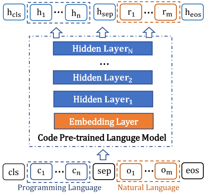
Figure 1: A typical CPLM.

2.2 Membership Inference

CMI is a specific type of membership inference (MI) Hu et al. (2022) which aims to ascertain whether a given data record is part of a particular dataset used to train a specific model. MI involves an adversary with access to both a trained machine learning model and a collection of input-output pairs, such as images and their corresponding labels. Although MI has been extensively studied Hu et al. (2022), CMI has received less attention and it is not easy to directly apply existing methods to CMI in the EaaS setting. Existing MI methods typically rely on the output logits of the target model Carlini et al. (2022); Mireshghallah et al. (2022); Ye et al. (2022); Li and Zhang (2021); Watson et al. (2022), which are not available for CMI in the EaaS setting since CPLMs generate embedding vectors instead of logits. Yang et al. Yang et al. (2023) train a surrogate model to mimic the target code generative model (e.g., CodeGPT), and then introduce a classifier to determine whether the input data is member or non-member. However, training a surrogate model requires considerable prior knowledge of the target model and it is resource-consuming. Besides, their approach focuses on code generative models, which are different from the CPLMs used in the EaaS setting.

3 Code Membership Inference in CPLMs

3.1 Task Definition

This paper studies CMI under the EaaS setting:

Definition 1 (Code Membership Inference)

Given token representations $\{\mathbf{h}_{1},\cdots,\mathbf{h}_{n}\}$ of a code snippet $c$ and possibly token representations $\{\mathbf{r}_{1},\cdots,\mathbf{r}_{m}\}$ of the corresponding natural language descriptions generated by the target CPLM $\mathcal{M}$, the adversary adopts an inference algorithm to determine whether $c$ is in the training data of $\mathcal{M}$.

Instead of giving “hard prediction”, the inference algorithm can output a continuous confidence score indicating the probability of $c$ being the code member data. Then, the adversary uses a threshold $\theta$ to yield the prediction:

$$\mathcal{A}(c)=\mathbbm{1}\left[\mathcal{I}(c)>\theta\right],$$ (1)

where $\mathbbm{1}$ is the indicator function, $\theta$ is a chosen threshold, $\mathcal{I}(\cdot)$ is the inference algorithm that produces the confidence score, and $\mathcal{A}(\cdot)$ is the membership indicator.

3.2 Knowledge Level

The knowledge of the adversary on $\mathcal{M}$ is critical to the success of CMI. To better study CMI, we define three knowledge levels as follows:

1. Complete Knowledge (i.e., White-Box Inference): The adversary has complete knowledge of $\mathcal{M}$ (e.g., model architecture and the trained model parameters). Moreover, the adversary can access a considerable amount of the training data (e.g., 70%). In practice, this is hard to achieve from the outside of EaaS provider.

2. Partial Knowledge (i.e., Gray-Box Inference): The adversary can access a small fraction (e.g., 5%) of the training data and know the core architecture (e.g., Transformer) of $\mathcal{M}$. Describing data sources (e.g., popular open-source libraries OpenAI (2021)) on the release website and data leaks Kammerath (2023) are common. Hence, this is a practical setting of CMI.

3. No Knowledge (i.e., Black-Box Inference): The adversary has the same information as other normal EaaS users (i.e., no prior knowledge). This is the most restricted setting of CMI.

3.3 Our Proposed Buzzer

This section illustrates the details of Buzzer. As depicted in Figs. 2, 3 and 4, Buzzer is designed for handling all the three settings of CMI.

3.3.1 White-Box Inference

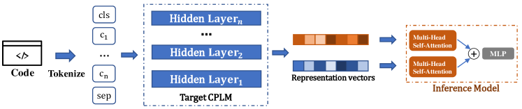
Figure 2: White-box inference. “$\oplus$” indicates the output vectors of the multi-head self-attention block are stacked.

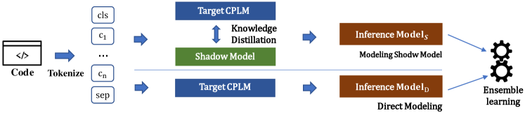
Figure 3: Gray-box inference.

Taking advantage of the prior knowledge on the considerable amount of training data, the adversary can train an inference model to infer code membership status. The adversary can mix known code member data and other code data (code non-member data) that is very unlikely to be the code member data to construct the inference model’s training data. Code non-member data can be collected from platforms or open-source libraries that are not included in the description of the training data sources of $\mathcal{M}$. This way, white-box inference becomes a binary classification problem.

The next question is how to define the behavior of $\mathcal{M}$ w.r.t. a certain code snippet $c$. Observed from Fig. 1 that the input tokens of $c$ are first encoded by the embedding layer and the embeddings are passed to the first hidden layer. There are multiple hidden layers in a CPLM, and each of them applies a non-linear function on the inputs from preceding layer. Hidden layers are key components that enable the CPLM to understand code data. Therefore, after feeding $c$ to $\mathcal{M}$, we can regards the outputs of hidden layers as the behavior of $\mathcal{M}$.

Fig. 2 depicts the white-box inference version of Buzzer. Buzzer first tokenizes $c$ and feeds it into $\mathcal{M}$. Then, it stacks the outputs from the layer in the middle and the last layer, which are most representative hidden layers, and feeds the result to the inference model which contains multi-head self-attention layers followed by a fully-connected layer used to produce the confidence score. Different layers can extract information at different levels. Hence, instead of only considering the last layer, we consider multiple layers to better depict the comprehensive behavior of $\mathcal{M}$.

3.3.2 Gray-Box Inference

Fig. 3 shows the gray-box inference version of Buzzer which requires a very small portion of code member data. Similar to white-box inference, we construct inference model’s training data by mixing the known code member data and the code non-member data. Differently, in gray-box inference, the adversary cannot access intermediate layers of $\mathcal{M}$ and can only receive token representations from the last layer of $\mathcal{M}$. This is the anticipated way for normal CPLM users to use the EaaS service to encode code data into high-dimensional representations Feng et al. (2020); Guo et al. (2021).

To model the behavior of $\mathcal{M}$, we design two strategies for gray-box inference:

Direct Modeling: A straightforward way is to simply use outputs from the last hidden layer of $\mathcal{M}$ to model its behavior. However, the last layer only produces the compressed representations and the states from intermediate layers are missing, making it difficult to accurately model the behavior of $\mathcal{M}$.

Modeling Shadow Model: The adversary can construct a shadow model to imitate $\mathcal{M}$ and extract outputs from the intermediate hidden layers of the shadow model as a substitute to capture $\mathcal{M}$’s behavior. To achieve this goal, we adopt response-based knowledge distillation (KD) Gou et al. (2021) and train the shadow model (student) to directly mimic the final output of $\mathcal{M}$ (teacher) by minimizing their divergence:

$$\mathcal{L}_{kd}=-{\sum_{c\in S}\sum_{t\in c}\left({\mathbf{h}^{\text{target}}_{t}-\mathbf{h}_{t}^{\text{shadow}}}\right)^{2}},$$ (2)

where $S$ is the known code member data and $t$ is a token in the code snippet $c$. $\mathbf{h}^{\text{target}}_{t}$ and $\mathbf{h}_{t}^{\text{shadow}}$ are outputs for $t$ from $\mathcal{M}$ and the shadow model, respectively. Since the adversary can not access the intermediate layers in $\mathcal{M}$, more sophisticated KD techniques (e.g., distill intermediate layers of $\mathcal{M}$) cannot be adopted. Since contemporary CPLMs mostly use the Transformer architecture, we adopt the RoBERTa-base architecture with 12 layers Liu et al. (2019) as the shadow model in order to ensure the compatibility between the teacher and the student.

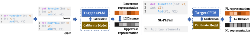
Figure 4: Black-box inference.

Note that direct modeling directly considers the (incomplete) signal from the last layer of $\mathcal{M}$, while modeling shadow model tries to construct the intermediate layers from the (incomplete) signal from $\mathcal{M}$. Therefore, both of them may suffer from the issue that the supervision (the incomplete signal only comes from the last layer of $\mathcal{M}$) may not be sufficient. To remedy this issue, we adopt the idea of ensemble learning Sagi and Rokach (2018) and train an ensemble inference model via stacking. A meta learner is used to combine the probability scores produced by the individual inference models such that the accuracy measure (i.e., the difference between the combined score and the ground-truth binary label) is maximized. We use logistic regression to achieve this goal and various established ensemble learning methods can be applied.

3.3.3 Black-Box Inference

As shown in Fig. 4, we develop two black-box inference versions of Buzzer without requiring inference data and inference model:

Unimodal Calibration: The adversary can perturb code data and discern its membership status based on the disparities in $\mathcal{M}$’s outputs. Let $\mathbf{h}_{\text{cls}}^{(\text{lower})}$ and $\mathbf{h}_{\text{cls}}^{(\text{upper})}$ be the produced representations of [CLS] for the lowercase version and the uppercase version of $c$. The representation of [CLS] is commonly used as the overall representation of the sequence. The adversary can measure the difference between $\mathbf{h}_{\text{cls}}^{(\text{lower})}$ and $\mathbf{h}_{\text{cls}}^{(\text{upper})}$ for black-box inference. If $c$ is code member data, $\mathcal{M}$ is likely to be more sensitive to its changes (i.e., large difference between $\mathbf{h}_{\text{cls}}^{(\text{lower})}$ and $\mathbf{h}_{\text{cls}}^{(\text{upper})}$). The reason is that CPLMs tend to memorize its training data well Carlini et al. (2023); Tirumala et al. (2022). CPLMS can perceive the small perturbation and produce quite different $\mathbf{h}_{\text{cls}}^{(\text{lower})}$ and $\mathbf{h}_{\text{cls}}^{(\text{upper})}$. We further use a calibration model to overcome the challenge of high false positive rate in MI, i.e., non-member samples are frequently predicted as member data Watson et al. (2022). The calibration model is based on RoBERTa-base architecture to promote its compatibility with the Transformer-based CPLM and it is trained on the code non-member data. We use the disparity of the generated representations of [CLS] from $\mathcal{M}$ and the calibration model to infer the membership status of $c$:

where $\left|\left|\cdot\right|\right|$ indicates the L2 distance. $\hat{\mathbf{h}}_{\text{cls}}^{(\text{lower})}$ and $\hat{\mathbf{h}}_{\text{cls}}^{(\text{upper})}$ are representations from the calibration model for [CLS] in the lowercase version and uppercase version, respectively. Using Eq. 3, for a code member snippet, the first term should be large and the second term should be small, resulting in a large $s_{\text{uni}}$. Reversely, for a code non-member snippet, the first term should be small while the second term can be small (the test code non-member snippet is non-overlapping with the non-member data used to train the calibration model) or large (the test code non-member snippet is overlapping with the non-member data used to train the calibration model). In either case, $s_{\text{uni}}$ should be small for a code non-member snippet. Therefore, using Eq. 3 can help reduce false positive rate.

Bimodal Calibration: CPLMs involves the natural language modality (NL) and the programming language modality (PL). The bimodal nature of CPLMs inspires us to leverage the discrepancy between two modalities for CMI. CPLMs are often pre-trained on PL-NL pairs Feng et al. (2020). A PL-NL pair consists of a code snippet and its corresponding method comment or other NL data. Intuitively, for PL-NL member pairs, the representations of the PL part and the NL part should be more close to each other than PL-NL non-member pairs since CPLMs are trained to associate code snippets with their corresponding NL descriptions. Similar to the unimodal calibration, we train a calibration model using RoBERTa-base. Differently, we concatenate the PL part and the NL part of a non-member PL-NL pair and use concatenated sequences to train the calibration model. We then use the disparity of the outputs from $\mathcal{M}$ and the calibration model to estimate the membership status of a test code snippet associated with some NL descriptions:

$$s_{\text{bi}}=\left|\left|\mathbf{h}_{\text{cls}}-\mathbf{r}_{\text{cls}}\right|\right|_{2}-\left|\left|\hat{\mathbf{h}}_{\text{cls}}-\hat{\mathbf{r}}_{\text{cls}}\right|\right|_{2},$$ (4)

where $\mathbf{h}_{\text{cls}}$ and $\mathbf{r}_{\text{cls}}$ are representations from $\mathcal{M}$ for the [CLS] token in the PL part and the NL part of the test code snippet, respectively. Similarly, $\hat{\mathbf{h}}_{\text{cls}}$ and $\hat{\mathbf{r}}_{\text{cls}}$ are outputs from the calibration model. Using Eq. 4, for a code member snippet, the first term should be small and the second term should be large, resulting in a small and possibly negative value of $s_{\text{bi}}$. On the contrary, for a code non-member snippet, the first term should be large while the second term can be large (the test code non-member snippet is non-overlapping with the non-member data used to train the calibration model) or small (the test code non-member snippet is overlapping with the non-member data used to train the calibration model). For the former case, $s_{\text{bi}}$ should be small for a code non-member snippet but it is possibly not as small as the score for the code member data which is very likely to be negative. For the later case, $s_{\text{bi}}$ should be large. Hence, using Eq. 4, Buzzer can distinguish code member data and code non-member data.

3.4 Threshold Selection

As illustrated in Eq. 1, the adversary needs to select the threshold $\theta$ of the confidence score to determine the membership status. We adapt the method proposed by Li and Zhang Li and Zhang (2021) and select the threshold for membership status on the validation set. In white-box inference and gray-box inference, since the adversary can access some code member data, we calculate the confidence scores of the known code member data and sort the scores. Then, the confidence score that is top-$k$ largest is selected as the threshold. In black-box setting, we calculate the confidence scores of the code non-member data and rank the scores. Then, the confidence score that is top-$g$ largest is selected as the threshold.

4 Experiments

4.1 Settings

4.1.1 Evaluation Metrics

We adopt Area Under the Curve (AUC) and accuracy (ACC) as evaluation metrics. They are widely used in evaluating MI Li and Zhang (2021); Mireshghallah et al. (2022); Zhang et al. (2021); Wang et al. (2022b). AUC assesses a model’s capability to differentiate between positive and negative samples by ranking output scores and calculating the probability of a sample being placed in the correct position. ACC directly evaluates the percentage of corrected predicted samples.

4.1.2 Data

We adopt four public code datasets CSN Husain et al. (2019), CoSQA Huang et al. (2021), PCSD Barone and Sennrich (2017) and DeepCom Hu et al. (2018). CSN is the code member dataset while the other three are code non-member dataset. The details of the data and the split of training/test/validation sets are provided in Appendix A. We check that there is no overlap between the member dataset and non-member dataset by comparing function names and similarities of code snippets.

4.1.3 CPLMs

We adopt four representative CPLMs CodeBERT Feng et al. (2020), GraphCodeBERT Guo et al. (2021), UniXcoder Guo et al. (2022) and CodeT5+ Wang et al. (2023) as target models. They were pre-trained on the CSN dataset. The details of these CPLMs are described in Appendix B.

4.1.4 Environment and Hyper-Parameters

Details of the environment and hyper-parameters are described in Appendix C.

4.2 Experimental Results

In this section, we analyze the effectiveness of Buzzer for CMI. We use the following notations to indicate different versions of Buzzer:

• CMI${}^{\text{wb}}$: It indicates Buzzer for white-box inference. Except for CodeT5+, outputs from the 6th and the 12th layers of $\mathcal{M}$ are used in the inference. For CodeT5+, the 10th and the 20th layers are used.

• CMI${}^{\text{gb}}_{\text{D}}$: In gray-box inference, only direct modeling is adopted to model the behavior of $\mathcal{M}$.

• CMI${}^{\text{gb}}_{\text{S(12)}}$: In gray-box inference, Buzzer uses the output of the 12th layer in the shadow model to capture the behavior of $\mathcal{M}$.

• CMI${}^{\text{gb}}_{\text{S(6+12)}}$: In gray-box inference, Buzzer uses the outputs of both 6th and 12th layers in the shadow model to capture the behavior of $\mathcal{M}$.

• CMI${}^{\text{gb}}_{\text{GBR}}$: Ensemble inference is adopted to combine CMI${}^{\text{gb}}_{\text{S(12)}}$ and CMI${}^{\text{gb}}_{\text{S(6+12)}}$ for gray-box inference. In this paper, for illustration, we adopt Gradient Boost Regression Friedman (2001) for ensemble learning.

• CMI${}^{\text{bb}}_{\text{uni}}$: It is black-box inference with unimodal calibration.

• CMI${}^{\text{bb}}_{\text{bi}}$: It is black-box inference with bimodal calibration.

4.2.1 Overall Performance

Table 1: Performance of white-box, gray-box and black-box inference for CPLMs.

CPLM	Dataset	AUC							ACC
		CMI${}^{\text{wb}}$	CMI${}^{\text{gb}}_{\text{S(12)}}$	CMI${}^{\text{gb}}_{\text{S(6+12)}}$	CMI${}^{\text{gb}}_{\text{D}}$	CMI${}^{\text{gb}}_{\text{GBR}}$	CMI${}^{\text{bb}}_{\text{uni}}$	CMI${}^{\text{bb}}_{\text{bi}}$	CMI${}^{\text{wb}}$	CMI${}^{\text{gb}}_{\text{S(12)}}$	CMI${}^{\text{gb}}_{\text{S(6+12)}}$	CMI${}^{\text{gb}}_{\text{D}}$	CMI${}^{\text{gb}}_{\text{GBR}}$	CMI${}^{\text{bb}}_{\text{uni}}$	CMI${}^{\text{bb}}_{\text{bi}}$
CodeBERT	PCSD	0.992	0.976	0.989	0.987	0.991	0.625	0.594	0.939	0.909	0.923	0.917	0.946	0.589	0.567
	CoSQA	0.938	0.918	0.927	0.93	0.936	0.575	0.719	0.858	0.837	0.854	0.858	0.844	0.564	0.655
	DeepCom	0.999	0.990	0.999	0.999	0.999	0.875	0.796	0.991	0.942	0.925	0.922	0.991	0.792	0.716
GraphCodeBERT	PCSD	0.992	0.986	0.985	0.988	0.989	0.621	0.661	0.929	0.908	0.913	0.908	0.917	0.585	0.621
	CoSQA	0.941	0.929	0.933	0.938	0.942	0.634	0.669	0.869	0.854	0.862	0.866	0.849	0.597	0.631
	DeepCom	0.999	0.999	0.999	0.999	0.999	0.730	0.734	0.998	0.932	0.918	0.904	0.992	0.658	0.666
UniXCoder	PCSD	0.991	0.891	0.968	0.925	0.971	0.567	0.599	0.918	0.767	0.892	0.840	0.911	0.545	0.572
	CoSQA	0.941	0.916	0.921	0.934	0.938	0.636	0.733	0.872	0.827	0.840	0.860	0.799	0.599	0.675
	DeepCom	0.999	0.960	0.989	0.999	0.999	0.713	0.732	0.975	0.885	0.916	0.935	0.915	0.649	0.670
CodeT5+	PCSD	0.975	0.909	0.971	0.944	0.974	0.609	0.769	0.904	0.896	0.896	0.864	0.911	0.585	0.647
	CoSQA	0.915	0.906	0.909	0.912	0.919	0.443	0.630	0.840	0.826	0.831	0.832	0.838	0.446	0.605
	DeepCom	0.999	0.999	0.999	0.999	0.999	0.461	0.695	0.923	0.925	0.933	0.931	0.996	0.486	0.705

Tab. 1 provides the overall experimental results of Buzzer. We can see that Buzzer generally achieves highest AUC and ACC in white-box inference (i.e., CMI${}^{\text{wb}}$), as it can access a considerable amount of code member data and use it to train an accurate inference model. As expected, gray-box inference (CMI${}^{\text{gb}}$) and black-box inference (CMI${}^{\text{bb}}$) show worse performance, since the adversary has much less prior knowledge of $\mathcal{M}$. Overall, except for CMI${}^{\text{bb}}_{\text{uni}}$ in some cases (discuss in Sec. 4.2.3), Buzzer can achieve promising CMI w.r.t. different CPLMs using different code non-member datasets.

To investigate whether Buzzer suffers from high false positive rate, we report the results of CMI${}^{\text{wb}}$, CMI${}^{\text{gb}}_{\text{GBR}}$ and CMI${}^{\text{bb}}_{\text{bi}}$ by separating the code member data and code non-member data in the test set in Tab. 2 where ACC${}_{\text{m}}$ represents the accuracy of classifying code member data correctly and ACC${}_{\text{n}}$ stands for the accuracy of classifying code non-member data correctly. We can see that Buzzer can overcome the high false positive rate issue, a common problem in existing MI works Watson et al. (2022) since the accuracy of classifying code non-member data correctly is high.

Table 2: ACC when separating code member and code non-member data in the test set.

Model	Dataset	CMI${}^{\text{wb}}$		CMI${}^{\text{gb}}_{\text{GBR}}$		CMI${}^{\text{bb}}_{\text{bi}}$
		ACCm	ACCn	ACCm	ACCn	ACCm	ACCn
CodeBERT	PCSD	0.876	0.998	0.907	0.985	0.517	0.616
	CoSQA	0.889	0.827	0.855	0.832	0.655	0.654
	DeepCom	0.999	0.982	0.982	0.999	0.725	0.706
GraphCodeBERT	PCSD	0.856	0.999	0.838	0.995	0.630	0.612
	CoSQA	0.861	0.882	0.923	0.775	0.679	0.582
	DeepCom	0.999	0.998	0.984	0.999	0.663	0.669
UniXCoder	PCSD	0.836	0.997	0.868	0.953	0.608	0.535
	CoSQA	0.884	0.851	0.951	0.647	0.640	0.709
	DeepCom	0.949	0.999	0.831	0.999	0.616	0.724
CodeT5+	PCSD	0.845	0.906	0.911	0.911	0.654	0.639
	CoSQA	0.829	0.859	0.838	0.837	0.627	0.566
	DeepCom	0.842	0.999	0.997	0.996	0.770	0.640

Table 3: Comparisons of using different combinations of hidden layers in the CPLM for white-box inference.

Layer(s)	Dataset	12		4+8		6+10		1+12		6+12		8+12
Model		ACC	AUC	ACC	AUC	ACC	AUC	ACC	AUC	ACC	AUC	ACC	AUC
CodeBERT	PCSD	0.913	0.983	0.926	0.990	0.910	0.991	0.924	0.985	0.920	0.990	0.920	0.989
	CoSQA	0.839	0.924	0.857	0.936	0.848	0.936	0.853	0.931	0.857	0.938	0.844	0.922
	DeepCom	0.930	0.999	0.941	0.999	0.917	0.999	0.951	0.999	0.917	0.999	0.927	0.999
GraphCodeBERT	PCSD	0.914	0.987	0.922	0.991	0.928	0.991	0.919	0.987	0.917	0.991	0.921	0.989
	CoSQA	0.852	0.932	0.850	0.938	0.856	0.938	0.859	0.934	0.866	0.941	0.854	0.935
	DeepCom	0.922	0.999	0.925	0.999	0.936	0.999	0.918	0.999	0.922	0.999	0.923	0.999
UniXcoder	PCSD	0.811	0.906	0.924	0.991	0.929	0.989	0.923	0.982	0.926	0.987	0.938	0.987
	CoSQA	0.858	0.932	0.858	0.935	0.853	0.930	0.859	0.933	0.859	0.936	0.829	0.931
	DeepCom	0.940	0.999	0.935	0.999	0.932	0.999	0.928	0.999	0.914	0.999	0.933	0.999

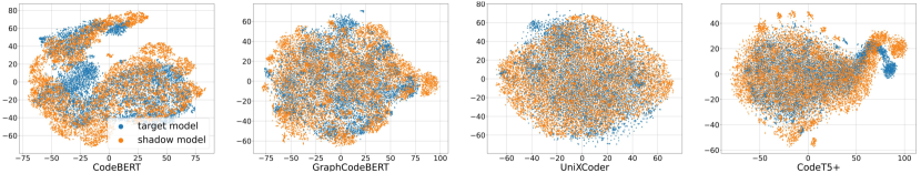
Figure 5: Visualization of the distribution of representations generated by the target model and the shadow model.

4.2.2 Analysis of Gray-Box Inference

Buzzer can perform three types of gray-box inference: directly modeling (CMI${}^{\text{gb}}_{\text{D}}$), modeling shadow model (CMI${}^{\text{gb}}_{\text{S}}$) and ensemble inference (CMI${}^{\text{gb}}_{\text{GBR}}$). From Tab. 1, we can observe that AUC and ACC of gray-box inference can generally achieve around 0.8-0.9. The observation shows that gray-box inference, which requires only a small portion of code member data that can be accessible in practice, can be achieved with high accuracy.

There are various options for directly modeling and modeling shadow model. In the following, we compare and discuss them in detail:

Necessity of Considering Intermediate Layers: We adopt KD to construct a shadow model in order to access its intermediate layers that are regards as the substitute of those of $\mathcal{M}$. It is necessary to investigate whether using multiple layers in $\mathcal{M}$ can improve the performance of inference compared to only using the last layer. Note that this results in a downgrade from CMI${}^{\text{gb}}_{\text{D}}$ for gray-box inference to CMI${}^{\text{wb}}$ for white-box inference.

Tab. 3 shows the results of CMI${}^{\text{wb}}$ on CodeBERT, GraphCodeBERT and UniXcoder when choosing different individual layer or the concatenation of multiple layers in $\mathcal{M}$. Since CodeT5+ has much more layers (20) than the other three CPLMs, its study is different and its result is reported in Appendix D. We can see that using a combination of outputs from one preceding layer and the last layer generally produce better inference than considering only one layer. Moreover, different combinations of outputs from two layers do no yield significant differences. We do not investigate more complicated combinations such as combining outputs from three or more layers since combining two layers already provides promising results (the results of AUC reach 0.999 in some cases) and using more layers causes higher computation cost. In summary, accessing the intermediate layers of $\mathcal{M}$ can increase the accuracy of CMI. Since such information is inaccessible in gray-box inference, using the intermediate hidden layer of the shadow model becomes an alternative and the KD step can help the adversary achieve this goal.

Feasibility of Using KD to Construct the Shadow Model: Since we use the shadow model as a substitute of $\mathcal{M}$, the large deviation between the distilled shadow model and $\mathcal{M}$ would violate our original intention of leveraging intermediate layers in $\mathcal{M}$ for gray-box inference. Thus, we compare directly modeling (CMI${}^{\text{gb}}_{\text{D}}$) and modeling shadow model (CMI${}^{\text{gb}}_{\text{S(6+12)}}$) to investigate whether KD will bring such a large deviation. From Tab. 1, we can observe that CMI${}^{\text{gb}}_{\text{S(6+12)}}$ generally outperforms CMI${}^{\text{gb}}_{\text{D}}$ w.r.t. ACC in most cases, although their AUC are close. Thus, it is feasible to use KD to construct a shadow model for gray-box inference.

Additionally, we randomly sample 10,000 code snippets from CSN and use $\mathcal{M}$ and the distilled shadow model to generate their representation. Then, we use TSNE Van der Maaten and Hinton (2008) to visualize the representations. As shown in Fig. 5, we can clearly observe that the representations from $\mathcal{M}$ and the distilled shadow model are similar as they cover similar regions in the plot. The observation again confirms the feasibility of using KD to construct a shadow model close to $\mathcal{M}$.

Comparisons of Ensemble Inference and Inference with a Single Strategy: As illustrated in Sec. 3.3.2, both directly modeling and modeling shadow model may suffer from the inadequate supervision and ensemble inference can be used to remedy this issue. By comparing the results of ensemble inference (CMI${}^{\text{gb}}_{\text{GBR}}$) and CMI${}^{\text{gb}}_{\text{D}}$/CMI${}^{\text{gb}}_{\text{S}}$ in Tabs. 1, we can observe that ensemble inference generally yield more accurate results, suggesting that ensemble learning can help overcome the inadequate supervision issue in gray-box inference.

4.2.3 Analysis of Black-Box Inference

From Tab. 1, we can see that AUC and ACC of Buzzer (CMI${}^{\text{bb}}_{\text{uni}}$ and CMI${}^{\text{bb}}_{\text{bi}}$) decrease significantly in black-box inference compared to the other two inference settings as no prior knowledge is available. Still, black-box inference is effective, as AUC and ACC of Buzzer still reach 0.6-0.7 in most cases, showing that Buzzer can still accurately identify code member data to some extend.

Moreover, we can see that CMI${}^{\text{bb}}_{\text{bi}}$ generally outperforms CMI${}^{\text{bb}}_{\text{uni}}$, showing the effectiveness of considering the bimodal nature of CPLMs. Particularly, for CodeT5+, CMI${}^{\text{bb}}_{\text{bi}}$ significantly exceeds CMI${}^{\text{bb}}_{\text{uni}}$. For CodeBERT on PCSD and DeepCom, CMI${}^{\text{bb}}_{\text{uni}}$ exhibits higher AUC and ACC than CMI${}^{\text{bb}}_{\text{bi}}$. Overall, the performance variance of CMI${}^{\text{bb}}_{\text{bi}}$ is smaller compared to CMI${}^{\text{bb}}_{\text{uni}}$: the gap between the maximum AUC and the minimum AUC of CMI${}^{\text{bb}}_{\text{bi}}$ is 0.202, whereas the gap for CMI${}^{\text{bb}}_{\text{uni}}$ is 0.432. Therefore, we can conclude that, for black-box inference, CMI${}^{\text{bb}}_{\text{bi}}$ is more effective and stable than CMI${}^{\text{bb}}_{\text{uni}}$.

4.2.4 Additional Experiments

We also study the influence of different code characteristics and impacts of different settings (the amount of known member data and different KD losses) on the inference results. Due to space limit, we report them in Appendix E and Appendix F.

5 Related Work

5.1 Code Pre-trained Language Model

Depending on the architecture, CPLMs can be categorized into encoder-only CPLMs, decoder-only CPLMs and encoder-decoder-based CPLMs. Encoder-only CPLMs typically follow the design of BERT Liu et al. (2019). CodeBERT Feng et al. (2020) uses masked language modeling and replaced token detection tasks for pre-training. GraphCodeBERT Guo et al. (2021) models code data from a structural perspective and it uses edge prediction and node alignment as the pre-training tasks. Some works consider the decoder-only design. IntelliCode Svyatkovskiy et al. (2020) and CodeGPT Lu et al. (2021) follow the objective of GPT-2, using the unidirectional language modeling task for pre-training. Besider, various CPLMs adopt the encoder-decoder architecture. UniXcoder Guo et al. (2022) utilizes prefix adapters to control the model behaviors and leverages multimodal data for enhancing performance. CodeT5 Wang et al. (2021) employs a unified framework to seamlessly support both code understanding and generation tasks and allows for multi-task learning. Recently, some CPLMs explore the power of large language model. Representative works like CodeT5+ Wang et al. (2023), StarCoder Li et al. (2023) and Code Llama Rozière et al. (2023) with billions of parameters show astounding performance on code-related tasks.

5.2 Membership Inference

Since the first MI study on genome data Homer et al. (2008), it has been studied by researchers in diverse domains, such as machine translation Hisamoto et al. (2020), recommender systems Wang et al. (2022b); Zhang et al. (2021), clinical models Mireshghallah et al. (2022); Jagannatha et al. (2021), and text classification Shejwalkar et al. (2021). As for language models, Song et al. Song and Raghunathan (2020) study MI for word embedding models. They distinguish member and non-member data by calculating the average similarity in a sliding window. Mahloujifar et al. Mahloujifar et al. (2021) leverage the semantic relationships preserved by word embeddings to identify special word pairs that are indicative of the presence of certain data in the training set. Jagannatha et al. Jagannatha et al. (2021) investigate the risk of training data leakage in clinical models. Mireshghallah et al. Mireshghallah et al. (2022) introduce a reference model and give the determination based on the likelihood ratio threshold.

6 Conclusion

In this paper, we study CMI for authenticating data compliance in CPLMs and propose a framework Buzzer for inferring code membership. Buzzer achieves promising results on various CPLMs as shown in the experiments. Hence, Buzzer can serve as a CMI tool and help protect the intellectual property rights. In the future, we plan to further improve the accuracy of black-box inference to achieve more practical CMI. We will also explore the idea of this work on other other multimodal pre-trained language models beyond CPLMs.

7 Limitations

We study CMI using public code data that is not originally designed for this task. In practice, the code data that their owners care about may contain core algorithms that are not publicly available, making it difficult to collect them for the study of CMI. For such cases, it is difficult to assess the performance of Buzzer based on the results reported in this paper.

Appendix A Details of Data

Four public datasets are used in our experiments:

• CSN Husain et al. (2019): CodeSearchNet (CSN) dataset contains over 6 million code snippets from open-source projects on GitHub, spanning six programming languages (Python, Java, JavaScript, Go, Ruby, and PHP). Code snippets are associated with metadata such code description written in natural language.

• CoSQA Huang et al. (2021): It comprises of more than 20,000 pairs of web queries and their corresponding python code, which are annotated by a minimum of three human annotators and tagged with a label signifying whether the code answers the query or not. This dataset is intended to serve as an exceptional resource for code search and question answering tasks.

• PCSD Barone and Sennrich (2017): The Python Code Summarization Dataset (PCSD) is a collection of parallel corpus consisting of Python functions and their corresponding NL descriptions (code comment). It comprises of 108,726 code-comment pairs extracted from open-source repositories on GitHub.

• DeepCom Hu et al. (2018): DeepCom is a Java corpus extracted from 9,714 open-source projects on GitHub. It is first used in code comment generation and contains pairs of code and comment strings.

It is known that prevalent CPLMs including the four CPLMs studied in this paper use CSN data in pre-training. Therefore, CSN is treated as code member data. We treat the remaining three datasets as code non-member data.

We prepare training/test/validation sets as follows:

1. White-Box Setting: We assume the adversary can access 70% code member data. We randomly sample 70% code member data and treat them as known member data to the adversary. The remaining 30% data is unknown member data. To construct the training set, we mix 30,000 code snippets sampled from the known member data and 30,000 code snippets sampled from the code non-member data. For the test set, we sample 10,000 code snippets from the unknown member data, and mix them with 10,000 code snippets sampled from code non-member data. For the validation set, we combine 500 code snippets sampled from the known member data and 500 code snippets sampled from the code non-member data.

2. Gray-Box Setting: The process is similar to white-box setting with the difference that known member data only accounts for 5% of the code member data.

3. Black-Box Setting: There is no training data. To construct the test set, we combine 10,000 code snippets sampled from the code member data and 10,000 code snippets sampled from the code non-member data. For the validation set, we sample 500 code snippets from the code non-member data.

Note that the adversary (i.e., the inference algorithm) can only access the training set and the validation set.

Appendix B Details of CPLMs

We adopt four representative CPLMs as target models in this study, including CodeBERT, GraphCodeBERT and UniXcoder developed by Microsoft and CodeT5+ developed by Salesforce:

• CodeBERT Feng et al. (2020): CodeBERT is a bimodal CPLM that uses transformer-based neural networks to learn high-quality code representations. It is pre-trained on massive code data with pre-trained tasks Masked Language Modeling and Random Token Detection.

• GraphCodeBERT Guo et al. (2021): GraphCodeBERT is a variant of CodeBERT and it incorporates the DFG of the code in the pre-training process. Instead of simply viewing code data as plain text sequence, GraphCodeBERT can better capture the structural information of code, leading to improved performance on various code-related tasks.

• UniXcoder Guo et al. (2022): UniXcoder is a unified, cross-modal CPLM that leverages multi-modal data such as code comments and ASTs in pre-training. To enhance the quality of code representations, UniXcoder introduces prefix adapters, which allow better control over the access to context for each token.

• CodeT5+ Wang et al. (2023): CodeT5+ follows the design of T5 Raffel et al. (2020) and adopts mixture of pre-training objectives to mitigate the discrepancy between pre-training and finetuning. We use the 2B version of CodeT5+ with 20 layers.

Appendix C Environment and Hyper-Parameters

We conduct our experiments using PyTorch and run the experiments on a machine with two Intel(R) Xeon(R) Silver 4214R CPU @ 2.40GHz, 256 GB main memory and one NVIDIA GeForce RTX 3090. The code features were extracted using the Python package tree-sitter. For shadow model modeling, we set the batch size to 32, while for the training stage of the inference model, the batch size is set to 128. The AdamW optimizer Loshchilov and Hutter (2019) with a learning rate of 0.01 is used for training. Code snippets and natural language comments are tokenized using Byte-Pair Encoding (BPE) Sennrich et al. (2016) used by RoBERTa-base Liu et al. (2019). For the threshold selection step explained in Sec. 3.4, we set $k=0.15$ and $g=0.6$.

Appendix D Impact of Using Different Layers in CodeT5+

Tab. 4 shows the results of CMI${}^{\text{wb}}$ on CodeT5+ with 20 layers when choosing different individual layer or the concatenation of multiple layers in $\mathcal{M}$. Similar to the results reported in Sec. 3, we can see that CodeT5+ using a combination of outputs from two layers generally produces better results than CodeT5+ considering only one layer. Besides, different combinations of outputs from two layers do no yield significant differences.

Table 4: Comparisons of using different combinations of hidden layers in CodeT5+ for white-box inference of CodeT5+.

Layer(s)	10		3+7		5+7		10+20
Dataset	ACC	AUC	ACC	AUC	ACC	AUC	ACC	AUC
PCSD	0.892	0.968	0.893	0.966	0.903	0.973	0.904	0.975
CoSQA	0.832	0.909	0.823	0.915	0.831	0.906	0.840	0.915
DeepCom	0.901	0.999	0.905	0.999	0.912	0.999	0.923	0.999

Appendix E Impact of Data Characteristics

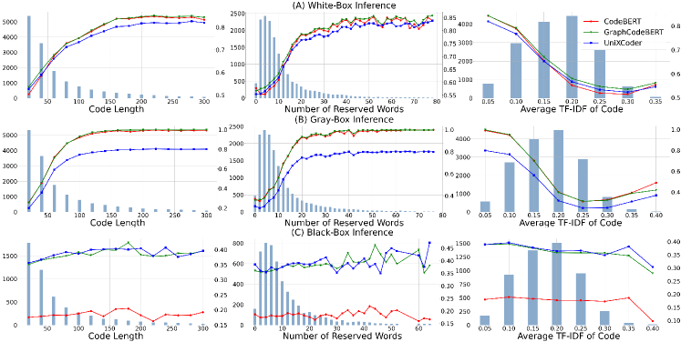
Figure 6: Distributions of the confidence scores of code snippets predicted by inference models.

In this section, we study the impacts of different code characteristics on the inference results. In other words, we are interested in the factors that affect how Buzzer makes membership status predictions. We investigate three common code features:

• Code Length: Code length refers to the length of a code snippet. Longer code snippets can provide more information,

• Number of Reserved Words: Reserved words are keywords that cannot be used as an identifier and may vary for different programming languages. For example, if, for, while, with, try and except are some reserved words in Python.

• Token Importance: We use the average TF-IDF value of all tokens in a code snippet to indicate how important tokens contained in the code snippet are.

Fig. 6 reports the distributions of the confidence scores of code snippets predicted by CMI${}^{\text{wb}}$, CMI${}^{\text{gb}}_{\text{GBR}}$ and CMI${}^{\text{bb}}_{\text{bi}}$ for white-box inference, gray-box inference and black-box inference, respectively. Due to space constraints, we only present the results using CoSQA as code non-member data. Initially, we obtain the values for the three features of each code snippet. Next, we group the code data into intervals with equal length, and arrange intervals in ascending order based on the corresponding feature. The x axis of Fig. 6 represents the intervals. The left y axis is the number of code samples in each interval and the right y axis denotes the confidence score. We normalize the scores to a range between 0 and 1 via min-max normalization. The bar charts in Fig. 6 represents the number of samples in each group, while the line graphs show the average confidence scores of each group. Subsequently, we examine the scores assigned by the inference model to different groups and analyze whether any specific patterns emerge across the intervals.

From the bars in Fig. 6, we can observe the long-tail distributions of code snippets grouped by code length and numbers of reserved words and the majority of code snippets have low values for code length and number of reserved words. Differently, the average TF-IDF scores of most code snippets are close to the median of the distribution (0.2).

Then, we consider both confidence scores and number of code snippets for each interval. We can find that, in white-box inference and gray-box inference, the predicted confidence scores are positively correlated with code length and number of reserve words, while they are roughly negatively correlated with average TF-IDF scores. The observation shows that, the three code features are strongly correlated with the inference results of Buzzer: code snippets with long length, more reserved keywords or small average TF-IDF scores are more likely to be predicted as code member data in white-box inference and gray-box inference.

However, the trend is different in black-box inference. Although some parts of the confidence score lines fluctuate, we can see that the variance of the confidence scores for each CPLM is not as significant as in white-box inference and gray-box inference (i.e., the confidence scores remain relatively stable as the values of code feature changes in black-box inference), suggesting that it is more difficult to find a suitable confidence score threshold to separate test code samples in black-box inference. This is the possible reason why Buzzer performs worse in black-box inference than in white-box and gray-box inference.

The above observations are consistent for the three CPLMs. But the level of confidence scores that Buzzer gives to a CPLM is different in the three types of inference. Code snippets receive lowest confidence scores on UniXCoder in white-box and gray-box inference, although their differences to scores on CodeBERT and GraphCodeBERT are marginal. Differently, in black-box inference, code snippets receive lowest confidence scores on CodeBERT and their their differences to scores on GraphCodeBERT and UniXCoder are remarkable. Hence, it is essential to select a score threshold for each CPLM in each inference type.

Appendix F Impacts of Different Settings

F.1 Impact of Known Member Data

The amount of known code member data should affect the quality of CMI. In this section, we take CMI${}^{\text{gb}}_{\text{S(12)}}$ as an example to investigate the influence of known data on Buzzer.

Tab. 5 reports the AUC results of CMI${}^{\text{gb}}_{\text{S(12)}}$ when it can access different percentage of code member data. Recall that, CMI${}^{\text{gb}}_{\text{S(12)}}$ can access 5% code member data in our default setting. Generally, acquiring more code member data helps improve the performance of CMI${}^{\text{gb}}_{\text{S(12)}}$. The improvements are noticeable for UniXCoder on DeepCom when the percentage increases from 3% to 10%. However, for most cases in Tab. 5, the performance of CMI${}^{\text{gb}}_{\text{S(12)}}$ is not very sensitive to the change of the percentage of known member data. One possible reason is that, using 5% code member data, CMI${}^{\text{gb}}_{\text{S(12)}}$ can already achieve accurate inference (0.8-0.9 for AUC) in the gray-box setting and more known data does not bring significant information gain.

Table 5: AUC of CMI${}^{\text{gb}}_{\text{S(12)}}$ when the percentage of known member data varies.

Model	Dataset	3%	5%	10%
CodeBERT	PCSD	0.972	0.976	0.986
	CoSQA	0.917	0.918	0.920
	DeepCom	0.999	0.990	0.999
GraphCodeBERT	PCSD	0.981	0.986	0.987
	CoSQA	0.927	0.929	0.930
	DeepCom	0.999	0.999	0.999
UniXCoder	PCSD	0.885	0.891	0.897
	CoSQA	0.900	0.916	0.915
	DeepCom	0.943	0.960	0.985
CodeT5p-2B	PCSD	0.961	0.971	0.981
	CoSQA	0.906	0.909	0.910
	DeepCom	0.986	0.999	0.999

Table 6: AUC of CMI${}^{\text{gb}}_{\text{S(12)}}$ when different losses are used.

Model	Dataset	COS	MSE	NST	PKD
CodeBERT	PCSD	0.984	0.976	0.981	0.960
	CoSQA	0.916	0.918	0.911	0.915
	DeepCom	0.999	0.990	0.999	0.999
GraphCodeBERT	PCSD	0.982	0.986	0.988	0.977
	CoSQA	0.930	0.929	0.921	0.930
	DeepCom	0.999	0.999	0.999	0.999
UniXCoder	PCSD	0.891	0.891	0.829	0.914
	CoSQA	0.912	0.916	0.889	0.907
	DeepCom	0.971	0.960	0.841	0.977
CodeT5p-2B	PCSD	0.961	0.971	0.981	0.981
	CoSQA	0.905	0.909	0.889	0.897
	DeepCom	0.998	0.999	0.785	0.779

F.2 Impact of Different KD Losses

Different KD losses can be adopted in CMI${}^{\text{gb}}_{\text{S}}$. Tab. 6 demonstrates the impact of using different loss functions for the construction of the shadow model. We report the results of CMI${}^{\text{gb}}_{\text{S(12)}}$ with widely used distillation losses MSE (i.e., Eq. 2), COS Sanh et al. (2019), NST Huang and Wang (2017), and PKD Sun et al. (2019). From the results in Tab. 6, we can see that the choice of loss function does not significantly affect the performance of code member inference. In most cases, the performance of MSE is similar to that of COS. NST and PKD generally yield worse performance compared to MSE and COS, but there are a few cases where they might perform better.

References

- Barone and Sennrich (2017) Antonio Valerio Miceli Barone and Rico Sennrich. 2017. A parallel corpus of python functions and documentation strings for automated code documentation and code generation. In IJCNLP(2), pages 314–319.
- Carlini et al. (2022) Nicholas Carlini, Steve Chien, Milad Nasr, Shuang Song, Andreas Terzis, and Florian Tramèr. 2022. Membership inference attacks from first principles. In IEEE Symposium on Security and Privacy, pages 1897–1914.
- Carlini et al. (2023) Nicholas Carlini, Daphne Ippolito, Matthew Jagielski, Katherine Lee, Florian Tramèr, and Chiyuan Zhang. 2023. Quantifying memorization across neural language models. In ICLR. https://openreview.net/pdf?id=TatRHT_1cK.
- Feng et al. (2020) Zhangyin Feng, Daya Guo, Duyu Tang, Nan Duan, Xiaocheng Feng, Ming Gong, Linjun Shou, Bing Qin, Ting Liu, Daxin Jiang, and Ming Zhou. 2020. Codebert: A pre-trained model for programming and natural languages. In EMNLP (Findings), pages 1536–1547.
- Friedman (2001) Jerome H Friedman. 2001. Greedy function approximation: a gradient boosting machine. Annals of statistics, pages 1189–1232.
- Google (2023) Google. 2023. Get text embeddings. https://cloud.google.com/vertex-ai/docs/generative-ai/embeddings/get-text-embeddings.
- Gou et al. (2021) Jianping Gou, Baosheng Yu, Stephen J. Maybank, and Dacheng Tao. 2021. Knowledge distillation: A survey. Int. J. Comput. Vis., 129(6):1789–1819.
- Guo et al. (2022) Daya Guo, Shuai Lu, Nan Duan, Yanlin Wang, Ming Zhou, and Jian Yin. 2022. Unixcoder: Unified cross-modal pre-training for code representation. In ACL (1), pages 7212–7225.
- Guo et al. (2021) Daya Guo, Shuo Ren, Shuai Lu, Zhangyin Feng, Duyu Tang, Shujie Liu, Long Zhou, Nan Duan, Alexey Svyatkovskiy, Shengyu Fu, Michele Tufano, Shao Kun Deng, Colin B. Clement, Dawn Drain, Neel Sundaresan, Jian Yin, Daxin Jiang, and Ming Zhou. 2021. Graphcodebert: Pre-training code representations with data flow. In ICLR. https://openreview.net/pdf?id=jLoC4ez43PZ.
- Hisamoto et al. (2020) Sorami Hisamoto, Matt Post, and Kevin Duh. 2020. Membership inference attacks on sequence-to-sequence models: Is my data in your machine translation system? Trans. Assoc. Comput. Linguistics, 8:49–63.
- Homer et al. (2008) Nils Homer, Szabolcs Szelinger, Margot Redman, David Duggan, Waibhav Tembe, Jill Muehling, John V Pearson, Dietrich A Stephan, Stanley F Nelson, and David W Craig. 2008. Resolving individuals contributing trace amounts of dna to highly complex mixtures using high-density snp genotyping microarrays. PLoS genetics, 4(8):e1000167.
- Hu et al. (2022) Hongsheng Hu, Zoran Salcic, Lichao Sun, Gillian Dobbie, Philip S. Yu, and Xuyun Zhang. 2022. Membership inference attacks on machine learning: A survey. ACM Comput. Surv., 54(11s):235:1–235:37.
- Hu et al. (2018) Xing Hu, Ge Li, Xin Xia, David Lo, and Zhi Jin. 2018. Deep code comment generation. In ICPC, pages 200–210.
- Huang et al. (2021) Junjie Huang, Duyu Tang, Linjun Shou, Ming Gong, Ke Xu, Daxin Jiang, Ming Zhou, and Nan Duan. 2021. Cosqa: 20, 000+ web queries for code search and question answering. In ACL/IJCNLP (1), pages 5690–5700.
- Huang and Wang (2017) Zehao Huang and Naiyan Wang. 2017. Like what you like: Knowledge distill via neuron selectivity transfer. arXiv Preprint. https://arxiv.org/abs/1707.01219.
- Husain et al. (2019) Hamel Husain, Ho-Hsiang Wu, Tiferet Gazit, Miltiadis Allamanis, and Marc Brockschmidt. 2019. Codesearchnet challenge: Evaluating the state of semantic code search. arXiv Preprint. https://arxiv.org/abs/1909.09436.
- InfoQ (2022) InfoQ. 2022. First open source copyright lawsuit challenges github copilot. https://www.infoq.com/news/2022/11/lawsuit-github-copilot/.
- Jagannatha et al. (2021) Abhyuday Jagannatha, Bhanu Pratap Singh Rawat, and Hong Yu. 2021. Membership inference attack susceptibility of clinical language models. arXiv Preprint. https://arxiv.org/abs/2104.08305.
- Kammerath (2023) Jan Kammerath. 2023. Copilot leaks: Code i should not have seen. https://medium.com/@jankammerath/copilot-leaks-code-i-should-not-have-seen-e4bda9b33ba6.
- Li et al. (2023) Raymond Li, Loubna Ben Allal, Yangtian Zi, Niklas Muennighoff, Denis Kocetkov, Chenghao Mou, Marc Marone, Christopher Akiki, Jia Li, Jenny Chim, Qian Liu, Evgenii Zheltonozhskii, Terry Yue Zhuo, Thomas Wang, Olivier Dehaene, Mishig Davaadorj, Joel Lamy-Poirier, João Monteiro, Oleh Shliazhko, Nicolas Gontier, Nicholas Meade, Armel Zebaze, Ming-Ho Yee, Logesh Kumar Umapathi, Jian Zhu, Benjamin Lipkin, Muhtasham Oblokulov, Zhiruo Wang, Rudra Murthy V, Jason Stillerman, Siva Sankalp Patel, Dmitry Abulkhanov, Marco Zocca, Manan Dey, Zhihan Zhang, Nour Moustafa-Fahmy, Urvashi Bhattacharyya, Wenhao Yu, Swayam Singh, Sasha Luccioni, Paulo Villegas, Maxim Kunakov, Fedor Zhdanov, Manuel Romero, Tony Lee, Nadav Timor, Jennifer Ding, Claire Schlesinger, Hailey Schoelkopf, Jan Ebert, Tri Dao, Mayank Mishra, Alex Gu, Jennifer Robinson, Carolyn Jane Anderson, Brendan Dolan-Gavitt, Danish Contractor, Siva Reddy, Daniel Fried, Dzmitry Bahdanau, Yacine Jernite, Carlos Muñoz Ferrandis, Sean Hughes, Thomas Wolf, Arjun Guha, Leandro von Werra, and Harm de Vries. 2023. Starcoder: may the source be with you! arXiv Preprint. https://arxiv.org/abs/2305.06161.
- Li and Zhang (2021) Zheng Li and Yang Zhang. 2021. Membership leakage in label-only exposures. In CCS, pages 880–895.
- Liu et al. (2023) Hao Liu, Yanlin Wang, Zhao Wei, Yong Xu, Juhong Wang, Hui Li, and Rongrong Ji. 2023. Refbert: A two-stage pre-trained framework for automatic rename refactoring. In ISSTA, pages 740–752.
- Liu et al. (2019) Yinhan Liu, Myle Ott, Naman Goyal, Jingfei Du, Mandar Joshi, Danqi Chen, Omer Levy, Mike Lewis, Luke Zettlemoyer, and Veselin Stoyanov. 2019. Roberta: A robustly optimized BERT pretraining approach. arXiv Preprint. https://arxiv.org/abs/1907.11692.
- Loshchilov and Hutter (2019) Ilya Loshchilov and Frank Hutter. 2019. Decoupled weight decay regularization. In ICLR (Poster). https://openreview.net/pdf?id=Bkg6RiCqY7.
- Lu et al. (2021) Shuai Lu, Daya Guo, Shuo Ren, Junjie Huang, Alexey Svyatkovskiy, Ambrosio Blanco, Colin B. Clement, Dawn Drain, Daxin Jiang, Duyu Tang, Ge Li, Lidong Zhou, Linjun Shou, Long Zhou, Michele Tufano, Ming Gong, Ming Zhou, Nan Duan, Neel Sundaresan, Shao Kun Deng, Shengyu Fu, and Shujie Liu. 2021. Codexglue: A machine learning benchmark dataset for code understanding and generation. In NeurIPS Datasets and Benchmarks.
- Mahloujifar et al. (2021) Saeed Mahloujifar, Huseyin A Inan, Melissa Chase, Esha Ghosh, and Marcello Hasegawa. 2021. Membership inference on word embedding and beyond. arXiv Preprint. https://arxiv.org/abs/2106.11384.
- Mireshghallah et al. (2022) Fatemehsadat Mireshghallah, Kartik Goyal, Archit Uniyal, Taylor Berg-Kirkpatrick, and Reza Shokri. 2022. Quantifying privacy risks of masked language models using membership inference attacks. In EMNLP, pages 8332–8347.
- OpenAI (2021) OpenAI. 2021. Openai codex. https://openai.com/blog/openai-codex.
- OpenAI (2023) OpenAI. 2023. Embeddings - use cases. https://platform.openai.com/docs/guides/embeddings/use-cases.
- Raffel et al. (2020) Colin Raffel, Noam Shazeer, Adam Roberts, Katherine Lee, Sharan Narang, Michael Matena, Yanqi Zhou, Wei Li, and Peter J. Liu. 2020. Exploring the limits of transfer learning with a unified text-to-text transformer. J. Mach. Learn. Res., 21:140:1–140:67.
- Rozière et al. (2023) Baptiste Rozière, Jonas Gehring, Fabian Gloeckle, Sten Sootla, Itai Gat, Xiaoqing Ellen Tan, Yossi Adi, Jingyu Liu, Tal Remez, Jérémy Rapin, Artyom Kozhevnikov, Ivan Evtimov, Joanna Bitton, Manish Bhatt, Cristian Canton-Ferrer, Aaron Grattafiori, Wenhan Xiong, Alexandre Défossez, Jade Copet, Faisal Azhar, Hugo Touvron, Louis Martin, Nicolas Usunier, Thomas Scialom, and Gabriel Synnaeve. 2023. Code llama: Open foundation models for code. arXiv Preprint. https://arxiv.org/abs/2308.12950.
- Sagi and Rokach (2018) Omer Sagi and Lior Rokach. 2018. Ensemble learning: A survey. WIREs Data Mining Knowl. Discov., 8(4).
- Sanh et al. (2019) Victor Sanh, Lysandre Debut, Julien Chaumond, and Thomas Wolf. 2019. Distilbert, a distilled version of BERT: smaller, faster, cheaper and lighter. arXiv Preprint. https://arxiv.org/abs/1910.01108.
- Sennrich et al. (2016) Rico Sennrich, Barry Haddow, and Alexandra Birch. 2016. Neural machine translation of rare words with subword units. In ACL (1), pages 1715–1725.
- Shejwalkar et al. (2021) Virat Shejwalkar, Huseyin A Inan, Amir Houmansadr, and Robert Sim. 2021. Membership inference attacks against nlp classification models. In NeurIPS 2021 Workshop Privacy in Machine Learning.
- Song and Raghunathan (2020) Congzheng Song and Ananth Raghunathan. 2020. Information leakage in embedding models. In CCS, pages 377–390.
- Sun et al. (2019) Siqi Sun, Yu Cheng, Zhe Gan, and Jingjing Liu. 2019. Patient knowledge distillation for BERT model compression. In EMNLP/IJCNLP (1), pages 4322–4331.
- Svyatkovskiy et al. (2020) Alexey Svyatkovskiy, Shao Kun Deng, Shengyu Fu, and Neel Sundaresan. 2020. Intellicode compose: code generation using transformer. In ESEC/SIGSOFT FSE, pages 1433–1443.
- Tirumala et al. (2022) Kushal Tirumala, Aram H. Markosyan, Luke Zettlemoyer, and Armen Aghajanyan. 2022. Memorization without overfitting: Analyzing the training dynamics of large language models. In NeurIPS, pages 38274–38290.
- Van der Maaten and Hinton (2008) Laurens Van der Maaten and Geoffrey Hinton. 2008. Visualizing data using t-sne. J. Mach. Learn. Res., 9(86):2579–2605.
- Vaswani et al. (2017) Ashish Vaswani, Noam Shazeer, Niki Parmar, Jakob Uszkoreit, Llion Jones, Aidan N. Gomez, Lukasz Kaiser, and Illia Polosukhin. 2017. Attention is all you need. In NIPS, pages 5998–6008.
- Wang et al. (2022a) Deze Wang, Zhouyang Jia, Shanshan Li, Yue Yu, Yun Xiong, Wei Dong, and Xiangke Liao. 2022a. Bridging pre-trained models and downstream tasks for source code understanding. In ICSE, pages 287–298.
- Wang et al. (2023) Yue Wang, Hung Le, Akhilesh Deepak Gotmare, Nghi D. Q. Bui, Junnan Li, and Steven C. H. Hoi. 2023. Codet5+: Open code large language models for code understanding and generation. arXiv Preprint. https://arxiv.org/abs/2305.07922.
- Wang et al. (2021) Yue Wang, Weishi Wang, Shafiq R. Joty, and Steven C. H. Hoi. 2021. Codet5: Identifier-aware unified pre-trained encoder-decoder models for code understanding and generation. In EMNLP (1), pages 8696–8708.
- Wang et al. (2022b) Zihan Wang, Na Huang, Fei Sun, Pengjie Ren, Zhumin Chen, Hengliang Luo, Maarten de Rijke, and Zhaochun Ren. 2022b. Debiasing learning for membership inference attacks against recommender systems. In KDD, pages 1959–1968.
- Watson et al. (2022) Lauren Watson, Chuan Guo, Graham Cormode, and Alexandre Sablayrolles. 2022. On the importance of difficulty calibration in membership inference attacks. In ICLR. https://openreview.net/pdf?id=3eIrli0TwQ.
- Yang et al. (2023) Zhou Yang, Zhipeng Zhao, Chenyu Wang, Jieke Shi, Dongsun Kim, DongGyun Han, and David Lo. 2023. Gotcha! this model uses my code! evaluating membership leakage risks in code models. arXiv Preprint. https://arxiv.org/abs/2310.01166.
- Ye et al. (2022) Jiayuan Ye, Aadyaa Maddi, Sasi Kumar Murakonda, Vincent Bindschaedler, and Reza Shokri. 2022. Enhanced membership inference attacks against machine learning models. In CCS, pages 3093–3106.
- Zhang et al. (2021) Minxing Zhang, Zhaochun Ren, Zihan Wang, Pengjie Ren, Zhumin Chen, Pengfei Hu, and Yang Zhang. 2021. Membership inference attacks against recommender systems. In CCS, pages 864–879.