Channel assisted noise propagation in a two-step cascade

Abstract

Signal propagation in biochemical networks is characterized by the inherent randomness in gene expression and fluctuations of the environmental components, commonly known as intrinsic and extrinsic noise, respectively. We present a theoretical framework for noise propagation in a generic two-step cascade (S$\rightarrow$X$\rightarrow$Y) in terms of intrinsic and extrinsic noise. We identify different channels of noise transmission that regulate the individual as well as the overall noise properties of each component. Our analysis shows that the intrinsic noise of S alleviates the overall noise and information transmission capacity along the cascade. On the other hand, the intrinsic noise of X and Y acts as a bottleneck of information transmission.

I Introduction

Noise plays an important role in shaping the dynamics of various cellular processes, including gene expression, transcriptional regulation, signal transduction pathways, and developmental pathways Kærn et al. (2005); Eldar and Elowitz (2010); Tsimring (2014). These cellular processes adopt diverse strategies in response to the inevitable influence of noise. Comprehension of the precise impact of noise on cellular processes is a complex endeavour and needs individual attention. In this context, exploring the influence of noise on regulatory cascades could reveal crucial insights into the role of noise in cellular functioning. Regulatory cascades are a common occurrence in biological systems, manifesting in various forms, one of which is transcriptional cascades in Escherichia coli and Saccharomyces cerevisiae Shen-Orr et al. (2002); Rosenfeld and Alon (2003). Moreover, cascades play a pivotal role in directing the temporal sequencing of gene expression, contributing to critical processes like sporulation McAdams and Shapiro (2003) and flagella formation Kalir et al. (2001). In more complex organisms like Drosophila and sea urchins, the developmental programs heavily rely on precisely orchestrated cascaded processes to achieve intricate temporal coordination of events Arnone and Davidson (1997); Davidson et al. (2002).

To address the propagation of noise in a cascade of gene expression, we consider the generic two-step cascade (TSC) S$\rightarrow$X$\rightarrow$Y representing gene regulatory network (GRN). Here, S, a transcription factor (TF), regulates the production of protein X which in turn regulates the production of protein Y. For associated kinetics and corresponding master equation we refer to Fig. 1a,b. TSC is a recurring architecture frequently found in more complex networks, often associated with additional control mechanisms Alon (2006); Ferrell (2022). Recent experimental investigation in synthetic transcriptional cascades having multiple stages of repression highlights the ability to exhibit ultrasensitive responses and low-pass filtering, resulting in robust behavior in input fluctuations Hooshangi et al. (2005). Furthermore, noise properties in steady-state using a framework of two-stage transcriptional cascades were examined Blake et al. (2003); Bruggeman et al. (2009); Maity et al. (2015).

The present communication characterises the noise propagation mechanism using the notion of noise decomposition, viz., intrinsic and extrinsic noise. The intrinsic noise is an inherent property of the system whereas the extrinsic noise is due to environmental fluctuations Elowitz et al. (2002). However, the characteristic distinction between intrinsic and extrinsic noise depends on the definition of the system Swain et al. (2002); Paulsson (2004, 2005); Hilfinger and Paulsson (2011). In a TSC, the intrinsic noise of each component (S, X , and Y) arises due to low copy number. On the other hand, the extrinsic noise in a component, say X, is accumulated due to noise coming from S. In this context, S is an extrinsic variable (“environment”) for X. Similarly, for Y, S and X both act as extrinsic variables (Fig. 1c).

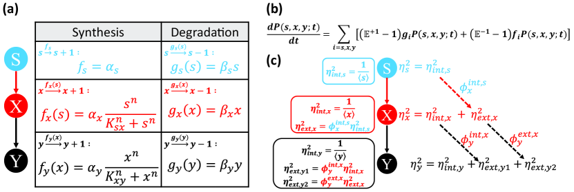
Figure 1: (color online) (a) Schematic of the kinetics of a generic two-step cascade. The synthesis and degradation of S is denoted by $f_{s}=\alpha_{s}$ and $g_{s}(s)=\beta_{s}s$, respectively, and resembles a simple birth-death process. $\alpha_{s}$ and $\beta_{s}$ are synthesis and degradation rate constants, with unit (molecules/V)min^-1 and min^-1, respectively. Synthesis of X and Y is characterized by ($s^{n}/(K_{sx}^{n}+s^{n})$ and $x^{n}/(K_{xy}^{n}+x^{n})$), respectively that captures the binding of the upstream regulator to the promoter of the downstream gene Alon (2006). $K_{ij}$ refers to the binding affinity of the upstream protein $i$ to the promoter of the downstream gene $j$ and $n$ is the Hill coefficient. The binding affinity $K_{ij}$ (expressed in molecules/V) defines a threshold in the concentration of $i$ necessary to significantly express the gene product $j$ Alon (2006). The rate constants $\alpha_{x}$ and $\alpha_{y}$ with unit (molecules/V)min^-1 take care of the synthesis of X and Y, respectively. The degradation of X and Y are linear functions with rate constants $\beta_{x}$ and $\beta_{y}$, respectively, with unit min^-1. In the text, $s$, $x$, and $y$ account for the copy number/volume of S, X, and Y, respectively. (b) Master equation corresponding to the kinetics given in (a) Gardiner (2009). $f_{i}$ and $g_{i}$ correspond to the synthesis and degradation functions of the system components, respectively. $\mathbb{E}^{\pm 1}$ are step operators whose action on a function of $s$, $x$, and $y$ gives a step-up ($\mathbb{E}^{+1}$) or step-down ($\mathbb{E}^{-1}$) in copy number. (c) Schematic of noise propagation from S to Y via X. The analytical expression of various intrinsic and extrinsic noise components are shown in Appendix C. Here, $\langle s\rangle$, $\langle x\rangle$, and $\langle y\rangle$ stand for the mean copy number of S, X, and Y, respectively, at steady state.

Investigating the role of intrinsic and extrinsic noise components in cellular functions, both in terms of their drawbacks Kærn et al. (2005) and advantagesRao et al. (2002); Eldar and Elowitz (2010); Herranz and Cohen (2010); Tsimring (2014), is therefore of great significance. Previous studies have suggested that both noise components (intrinsic and extrinsic) can act as degrading factors in information transmission in cellular responses Tkačik et al. (2008); Cheong et al. (2011); Uda et al. (2013); Selimkhanov et al. (2014); Voliotis et al. (2014); Garner et al. (2017); Potter et al. (2017); Suderman et al. (2017); Granados et al. (2018). However, a recent communication shows enhancement of information transmission due to cell-to-cell variability (extrinsic noise in this context) in skeletal muscle Wada et al. (2020). We note that mutual information (MI), a measure of statistical dependency between two variables in information theory quantifies information transmission capacity Shannon (1948); Shannon and Weaver (1963); Cover and Thomas (1991).

Regulatory cascades in biological systems have long been recognized for their critical role in transmitting information and orchestrating various cellular processes. However, the extent to which intrinsic and extrinsic noise contribute to the transmission of information within these cascades remains relatively unexplored. The present study aims to address this gap by considering the intrinsic and extrinsic noise components as well as decomposing the extrinsic noise of the final gene product Y (Fig. 1c). Our analysis identifies distinct noise processing channels that actively govern the propagation of noise along the cascade. We also delve into the impact of each decomposed noise term on information transmission along the cascade. Despite the apparent simplicity in the architecture, the TSC reveals an intricate relationship between noise and information, offering valuable insights into the underlying mechanisms that govern cellular functions and dynamics.

II The model and methods

The stochastic kinetics of a generic TSC is given by

$$s\stackrel{{\scriptstyle f_{s}}}{{\longrightarrow}}s+1,\;\;\;x\stackrel{{\scriptstyle f_{x}(s)}}{{\longrightarrow}}x+1,\;\;\;y\stackrel{{\scriptstyle f_{y}(x)}}{{\longrightarrow}}y+1,$$ (1a)

$$s\stackrel{{\scriptstyle g_{s}(s)}}{{\longrightarrow}}s-1,\;\;\;x\stackrel{{\scriptstyle g_{x}(x)}}{{\longrightarrow}}x-1,\;\;\;y\stackrel{{\scriptstyle g_{y}(y)}}{{\longrightarrow}}y-1,$$ (1b)

where $s$, $x$, and $y$ stand for the copy number/volume of S, X, and Y, respectively. Here $f_{i}$ and $g_{i}$ ($i\equiv s,x,y$) correspond to the synthesis and degradation functions of the system components, respectively. The explicit expressions of $f_{i}$ and $g_{i}$ are outlined in Fig. 1a. The master equation following the stochastic kinetics outlined in Eq. (1) is Gardiner (2009)

$$\frac{dP(s,x,y;t)}{dt} = \sum_{i=s,x,y}\left[(\mathbb{E}^{+1}-1)g_{i}P(s,x,y;t)\right.$$ (2)

$$\left.+(\mathbb{E}^{-1}-1)f_{i}P(s,x,y;t)\right].$$

In the above equation, $\mathbb{E}^{\pm}$ refers to the step operator which either step-up ($\mathbb{E}^{+1}$) or step-down ($\mathbb{E}^{-1}$) the copy numbers of the respective components by unity. We employ van Kampen’s system size expansion van Kampen (2007) to derive the Lyapunov equation (see Appendix A) which provides the statistical moments associated with the TSC (see Appendix B).

II.1 Noise decomposition in a two-step cascade

In a GRN, the noise associated with the $i$-th node is measured by the square of coefficient of variation, $\eta_{i}^{2}=\sigma_{i}^{2}/\langle i\rangle^{2}$. As per the noise decomposition formalism $\eta_{i}^{2}$ can be written as $\eta_{i}^{2}=\eta_{int,i}^{2}+\eta_{ext,i}^{2}$ Elowitz et al. (2002); Swain et al. (2002); Paulsson (2005); Hilfinger and Paulsson (2011) where $\eta_{int,i}^{2}$ and $\eta_{ext,i}^{2}$ are intrinsic and extrinsic noise, respectively. The intrinsic noise $\eta_{int,i}^{2}$ arises due to the birth-death processes whereas the extrinsic noise $\eta_{ext,i}^{2}$ is fed from its upstream regulator. The noise associated with the nodes S, X and Y of a TSC is (see Appendix C)

$$\eta_{s}^{2} = \eta_{int,s}^{2},$$ (3)

$$\eta_{x}^{2} = \eta_{int,x}^{2}+\eta_{ext,x}^{2},$$ (4)

$$\eta_{y}^{2} = \eta_{int,y}^{2}+\eta_{ext,y1}^{2}+\eta_{ext,y2}^{2}.$$ (5)

In Eq. (3), S contains only intrinsic noise ($\eta_{int,s}^{2}$) due to the Poisson kinetics. The noise associated with X, however, contains both intrinsic ($\eta_{int,x}^{2}$) and extrinsic parts ($\eta_{ext,x}^{2}$). The extrinsic noise $\eta_{ext,x}^{2}$ arises due to the propagation of noise from S to X, i.e., from $\eta_{int,s}^{2}$. Similarly, the total noise of Y, $\eta_{y}^{2}$, has intrinsic noise $\eta_{int,y}^{2}$ and a summation of two extrinsic noises $\eta_{ext,y1}^{2}$ and $\eta_{ext,y2}^{2}$. The source of extrinsic noise $\eta_{ext,y1}^{2}$ is the intrinsic noise $\eta_{int,x}^{2}$. On the other hand, $\eta_{ext,y2}^{2}$ is generated due to the contribution of $\eta_{ext,x}^{2}$. We refer to Fig. 1c for the flow of noise along the cascade. We note that the noise decomposition technique is general for Hill coefficient $n\geqslant 1$ and can be extended to a linear cascade with nodes $\geqslant 3$.

For $n=1$ the explicit expressions of the extrinsic noise given in Eqs. (3-5) are (see Appendix C)

$$\eta_{ext,x}^{2} = \phi_{x}^{int,s}\eta_{int,s}^{2},$$ (6)

$$\eta_{ext,y1}^{2} = \phi_{y}^{int,x}\eta_{int,x}^{2},$$ (7)

$$\eta_{ext,y2}^{2} = \phi_{y}^{ext,x}\eta_{ext,x}^{2}=\phi_{y}^{ext,x}\phi_{x}^{int,s}\eta_{int,s}^{2},$$ (8)

where,

$$\phi_{x}^{int,s} = \tau_{x,s}\left(\frac{K_{sx}}{K_{sx}+\langle s\rangle}\right)^{2},$$ (9)

$$\phi_{y}^{int,x} = \tau_{y,x}\left(\frac{K_{xy}}{K_{xy}+\langle x\rangle}\right)^{2},$$ (10)

$$\phi_{y}^{ext,x} = \tau_{sy,x}^{-1}\phi_{y}^{int,x}.$$ (11)

Eqs. (6-8) suggest that the quantity $\phi$ measures the fraction of upstream noise propagated to its corresponding downstream node. Depending on the cascade architecture and the model parameters, $\phi$ quantitates the pool of noise that flows downstream (see Eqs. (9-11)). To be specific, $\phi_{x}^{int,s}$ quantifies the fraction of intrinsic noise of S transmitted to X that builds up the extrinsic noise pool of X, $\eta_{ext,x}^{2}$ (Fig. 1c). $\phi_{y}^{int,x}$ measures the fraction of intrinsic noise of X propagated to Y to generate the extrinsic noise pool $\eta_{ext,y1}^{2}$ of Y (Fig. 1c). Similarly, $\phi_{y}^{ext,x}$ measures the fraction of extrinsic noise of X that flows down to Y and generates the second part of the extrinsic noise pool $\eta_{ext,y2}^{2}$ of Y (Fig. 1c). The measure $\phi$, thus, characterizes the noise transmission channels between different nodes of the cascade and identifies how noise propagation influences various species of the linear cascade. It is important to mention that $\phi$ always remains $<1$ independent of various model parameters.

In Eqs. (9-11), $\tau$-s are the scaled time scale Paulsson (2004, 2005) defined as $\tau_{i,j}:=\beta_{i}/(\beta_{i}+\beta_{j})$ and $\tau_{ij,k}:=(\beta_{i}+\beta_{j})/(\beta_{i}+\beta_{j}+\beta_{k})$ where $\beta_{i}$ ($i\in\{s,x,y\}$) corresponds to the degradation rate constant of the $i$-th species. The expressions of $\tau$-s indicate that $\tau_{x,s}<1$, $\tau_{y,x}<1$, and $\tau_{sy,x}<1$. Moreover, the second factors in Eqs. (9,10) are also less than unity. This results in $\phi_{x}^{int,s}<1$ and $\phi_{y}^{int,x}<1$. On the other hand, although $\tau_{sy,x}^{-1}>1$, we assume that this factor will not overpower $\phi_{y}^{int,x}$, which is much less than one, and hence leads to $\phi_{y}^{ext,x}<1$. This assumption remains valid as long as the separation of degradation time scale is maintained, i.e., $\beta_{s}\ll\beta_{x}\ll\beta_{y}$. The separation of degradation time scale maintains a maximum level of noise propagation along the cascade Maity et al. (2015).

The noise propagation from S to X opens up a single noise propagation channel characterized by $\phi_{x}^{int,s}$. On the other hand, noise transmission from X to Y is regulated by two different channels $\phi_{y}^{int,x}$ and $\phi_{y}^{ext,x}$. Noise flow from S to Y via X is characterized by $\phi_{x}^{int,s}$ and $\phi_{y}^{ext,x}$. We note that an increase of cascade length opens up multiple new channels of noise propagation. For example, in a cascade S$\rightarrow$X$\rightarrow$Y$\rightarrow$Z, additional downstream channels open up for noise propagation from Y to Z.

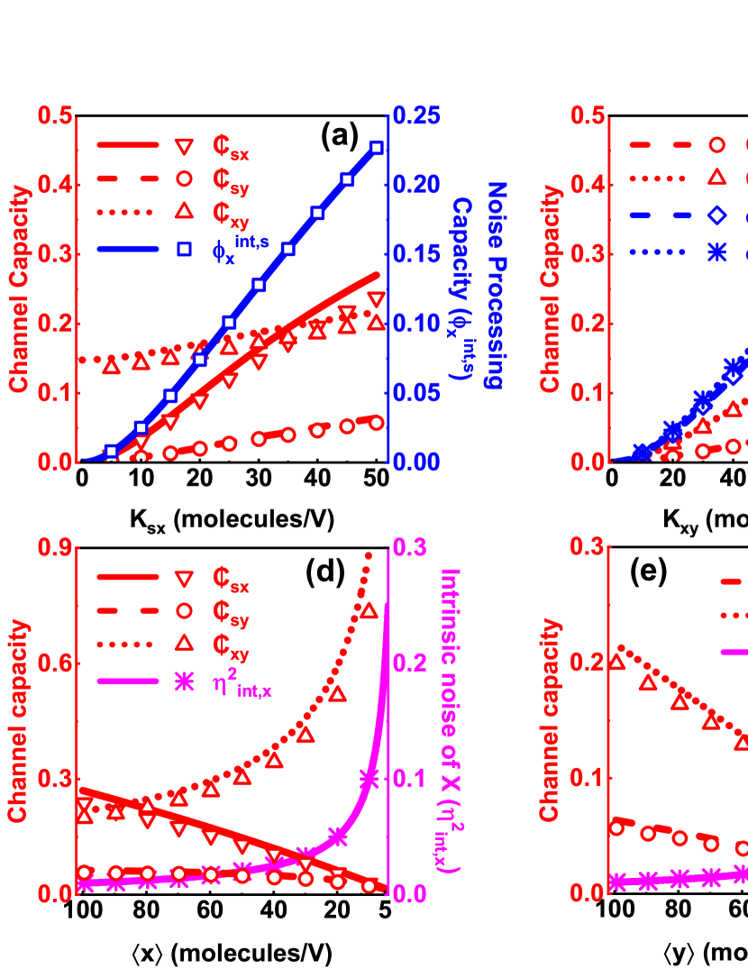
Figure 2: (color online) (a,b) Variations in channel capacity and noise processing capacity $\phi$ as a function of $K_{sx}$ and $K_{xy}$. The parameters used are $\beta_{s}=0.1$ min^-1, $\beta_{x}=1.0$ min^-1, $\beta_{y}=10.0$ min^-1, $\langle s\rangle=50.0$ molecules/V, $\langle x\rangle=100.0$ molecules/V, $\langle y\rangle=100.0$ molecules/V, and $n=1$. For (a) $K_{xy}=\langle x\rangle$ and for (b) $K_{sx}=\langle s\rangle$. (c-e) Variations in channel capacity and intrinsic noise of S, X, and Y as a function of mean copy number. The parameters used are $\beta_{s}=0.1$ min^-1, $\beta_{x}=1.0$ min^-1, $\beta_{y}=10.0$ min^-1, $K_{sx}=\langle s\rangle$, $K_{xy}=\langle x\rangle$, and $n=1$. For (c) $\langle x\rangle=100.0$ molecules/V and $\langle y\rangle=100.0$ molecules/V. For (d) $\langle s\rangle=50.0$ molecules/V and $\langle y\rangle=100.0$ molecules/V, and for (e) $\langle s\rangle=50.0$ molecules/V and $\langle x\rangle=100.0$ molecules/V. In (a-e), the lines are due to theoretical expression and the symbols are generated by numerical simulation using stochastic simulation algorithm Gillespie (1976, 1977). (f) Schematic presentation of channel capacities in a TSC and the role of intrinsic noise on information propagation. The pointed and blunt arrowheads stand for activation and repression, respectively.

III Results and discussion

The notion of mutual information Shannon (1948); Shannon and Weaver (1963) is used to address the interplay between noise and information transmission. The mutual information between two random variables $i$ and $j$ is written as $I(j;i):=\sum_{i,j}p(i,j)\log_{2}[p(i,j)/p(i)p(j)]$, where $p(i)$ and $p(j)$ are marginal probability distributions and $p(i,j)$ refer to the joint probability distribution of the variables Cover and Thomas (1991). For a bivariate system $i$ and $j$ obeying Gaussian statistics, the channel capacity is $\mathbb{C}_{ij}:=I(i;j)=(1/2)\log_{2}[1+\mathbb{S}_{ij}]$, where $\mathbb{S}_{ij}$ ($=\eta_{ij}^{4}/(\eta_{i}^{2}\eta_{j|i}^{2})$) is the signal-to-noise ratio (SNR) of the respective channels Tostevin and ten Wolde (2010). Here $\eta_{ji}^{2}$, $\eta_{i}^{2}$, and $\eta_{j|i}^{2}$ stand for the normalised covariance ($\sigma_{ji}^{2}/(\langle j\rangle\langle i\rangle)$), variance $(\sigma_{i}^{2}/\langle i\rangle^{2}$) and conditional variance ($\sigma_{j|i}^{2}/\langle j\rangle^{2}$), respectively (see Appendix D for the explicit expressions of $\mathbb{S}_{ij}$ and $\mathbb{C}_{ij}$). In the present scenario, we have three possible information processing channels, i.e., S$\rightarrow$X, X$\rightarrow$Y, and the overall channel S$\rightarrow$X$\rightarrow$Y.

For $\beta_{s}\ll\beta_{x}\ll\beta_{y}$ the scaled time scales $\tau$-s become approximately equal to 1 (see Appendix D). In this limit the analytical expressions of channel capacities are,

$$\mathbb{C}_{sx} = \frac{1}{2}\log_{2}\left[1+\frac{\phi_{x}^{int,s}\eta_{int,s}^{2}}{\eta_{int,x}^{2}}\right],$$ (12)

$$\mathbb{C}_{sy} = \frac{1}{2}\log_{2}\left[1+\frac{\phi_{x}^{int,s}\phi_{y}^{ext,x}\eta_{int,s}^{2}}{\eta_{int,y}^{2}+\phi_{y}^{int,x}\eta_{int,x}^{2}}\right],$$ (13)

$$\mathbb{C}_{xy} = \frac{1}{2}\log_{2}\left[1+\frac{A}{B}\right],$$ (14)

where

$$A = \phi_{y}^{int,x}\eta_{int,x}^{4}+(\phi_{x}^{int,s}\eta_{int,s}^{2}+2\eta_{int,x}^{2})\phi_{x}^{int,s}\phi_{y}^{ext,x}\eta_{int,s}^{2},$$

$$B = \eta_{int,x}^{2}\eta_{int,y}^{2}+(\eta_{int,y}^{2}+\phi_{y}^{int,x}\eta_{int,x}^{2})\phi_{x}^{int,s}\eta_{int,s}^{2}$$

$$-\phi_{x}^{int,s}\phi_{y}^{ext,x}\eta_{int,s}^{2}\eta_{int,x}^{2}.$$

As the input signal S acts as an extrinsic variable for both X and Y, increase in $\phi_{x}^{int,s}$ amplifies all three channel capacities, $\mathbb{C}_{sx}$, $\mathbb{C}_{sy}$, and $\mathbb{C}_{xy}$ (see Eqs. (12-14)). Notably, $\mathbb{C}_{sx}$ exhibits the most rapid increase in response to variations in $\phi_{x}^{int,s}$ compared to $\mathbb{C}_{sy}$ and $\mathbb{C}_{xy}$ (Fig. 2a). On the other hand, for X$\rightarrow$Y channel, X acts as an extrinsic variable for Y. Therefore, an increase in $\phi_{y}^{int,x}$ and $\phi_{y}^{ext,x}$ leads to enhancement of the channel capacities $\mathbb{C}_{sy}$ and $\mathbb{C}_{xy}$ (see Eqs. (13,14) and Fig. 2b). These findings illustrate that the magnitude of $\phi$-s, which characterizes noise propagation along each channel, is closely associated with the information transmission capacity of each channel. $\phi$ thus serves as an indicator of the noise processing capacity of individual noise processing channels along the regulatory edges.

The noise processing capacity $\phi$ generates an extrinsic noise pool at the downstream node of each channel which enhances information transmission along the respective channel. Therefore, it can be argued that the contribution of extrinsic noise at the downstream node plays a positive role in facilitating information transmission from an upstream node. Eq. (12-14) further reveals that the intrinsic noise $\eta_{int,s}^{2}$ enhances all the three channel capacities (Fig. 2c,f). The input noise $\eta_{int,s}^{2}$ thus facilitates information transmission downstream as it acts as an extrinsic variable for X and Y. In other words, the more the magnitude of $\eta_{int,s}^{2}$, more the downstream nodes X and Y sense the input noise as information.

The influence of the intrinsic noise of X ($\eta_{int,x}^{2}$) on $\mathbb{C}_{sx}$ and $\mathbb{C}_{sy}$ is repressing in nature (Fig. 2d,f). The increase in intrinsic noise of X acts as a constraint, limiting X’s ability to accurately detect the signal S and consequently, the information transmission from S to X ($\mathbb{C}_{sx}$) diminishes. The information transmission from S to Y ($\mathbb{C}_{sy}$) also diminishes as Y gains information from S via X. The information transmission from X to Y ($\mathbb{C}_{xy}$) increases due to $\eta_{int,x}^{2}$ (Fig. 2d,f) as $\eta_{int,x}^{2}$ acts as an extrinsic variable for the channel X$\rightarrow$Y. The intrinsic noise of Y, $\eta_{int,y}^{2}$, increases the variability of Y. As a consequence, $\eta_{int,y}^{2}$ acts as a potent limiting factor for which the information gained by Y from both S and X ($\mathbb{C}_{sy}$ and $\mathbb{C}_{xy}$) is reduced (Fig. 2e,f).

IV Conclusion

To summarize, we presented a theoretical analysis of noise propagation in a TSC on the basis of noise decomposition, and demonstrated the presence of distinct noise processing channels between the system components S, X, and Y. The extent of noise propagation along these channels depends on the noise processing capacity $\phi$. The intrinsic noise of the signal $\eta_{int,s}^{2}$ together with noise processing capacities ($\phi$) act as extrinsic variables and alleviates the overall information transmission along the cascade. On the other hand, the intrinsic noise of X, $\eta_{int,x}^{2}$ put a limit in information transmission along the channels S$\rightarrow$X and S$\rightarrow$X$\rightarrow$Y and act as bottleneck that reduce information transfer capacities. Similarly, intrinsic noise of Y, $\eta_{int,y}^{2}$ hinders information flow along the channels S$\rightarrow$X$\rightarrow$Y and X$\rightarrow$Y. Thus, noise propagation along the TSC depends on noise processing capacity of each noise processing channels which along with intrinsic noises modulate the information transmission capacity of the system.

The interplay between intrinsic and extrinsic noise constitutes an optimum signal transduction machinery. When there is a need to precisely sense and detect the signal for adaptability, the genes within the cascade exhibit dynamics in which the molecular intrinsic fluctuations become negligible. This ensures that the inherent noise of the system does not hinder the accurate reception of the signal. Conversely, when the signal is detrimental to the cellular response, the cascade’s gene expression dynamics adapt in a manner that increases the intrinsic noise of the gene products. Such strategy can be seen as a protective mechanism, where the system becomes less responsive to external fluctuations thereby prioritizing robustness that might otherwise disrupt its normal functioning.

Appendix A System size expansion and Lyapunov equation

In the following, we use the notation $\mathbf{N}$ to represent a three dimensional vector of copy numbers of the components, i.e., $\mathbf{N}\in\{n_{s}\equiv s,n_{x}\equiv x,n_{y}\equiv y\}$. We rewrite Eq. (2) in terms of macroscopic concentration of each component defined as $c_{i}:=\lim\limits_{\Omega\to\infty}(n_{i}/\Omega)$ with $i\in\{s,x,y\}$ Hayot and Jayaprakash (2004); van Kampen (2007) where $\Omega$ is the reaction volume,

$$\frac{dP(\boldsymbol{N};t)}{dt} = \Omega\sum_{i=s,x,y}\left[(\mathbb{E}_{i}^{+1}-1)g_{i}(n_{i}/\Omega)P(\boldsymbol{N};t)\right.$$ (15)

$$\left.+(\mathbb{E}_{i}^{-1}-1)f_{i}(\boldsymbol{N}/\Omega)P(\boldsymbol{N};t)\right].$$

In the above equation, $f_{i}(\boldsymbol{N}/\Omega)$ represents the generalised form of any reaction network. For TSC it specifically translates to $f_{s}$, $f_{x}(n_{s}/\Omega)$, and $f_{y}(n_{x}/\Omega)$, representing the production of S, X, and Y, respectively. In the following, we provide the pedagogical formulation of van Kampen’s system size expansion van Kampen (2007) to solve the Eq. (15). We now expand $n_{i}$ in $\Omega$ space of $\mathcal{O}(\Omega^{1/2})$

$$n_{i}=\Omega c_{i}+\Omega^{1/2}\epsilon_{i},$$ (16)

where $\epsilon_{i}$ represents the fluctuations around $n_{i}$. Using Eq. (16) in the left hand side of Eq. (15) we have

$$\frac{dP(\boldsymbol{N};t)}{dt}=\frac{d\widetilde{P}(\boldsymbol{\epsilon};t)}{dt}-\Omega^{-1/2}\sum_{i=s,x,y}\frac{dc_{i}}{dt}\frac{d\widetilde{P}(\boldsymbol{\epsilon};t)}{d\epsilon_{i}},$$ (17)

with $\boldsymbol{\epsilon}\in\{\epsilon_{s},\epsilon_{x},\epsilon_{y}\}$. Eq. (17) accounts for the time derivative of $P(\boldsymbol{N};t)$ at fixed $n_{i}$ so that Eq. (16) becomes $(d\epsilon_{i}/dt)=\Omega^{-1/2}(dc_{i}/dt)$ Elf and Ehrenberg (2003); Hayot and Jayaprakash (2004). Expansion of the step operator $\mathbb{E}^{\pm}$ in Eq. (15) provides Elf and Ehrenberg (2003); Hayot and Jayaprakash (2004)

$$\mathbb{E}_{i}^{+1} = 1+\Omega^{-1/2}(\partial/\partial\epsilon_{i})+(1/2)\Omega^{-1}(\partial^{2}/\partial\epsilon_{i}^{2}),$$ (18)

$$\mathbb{E}_{i}^{-1} = 1-\Omega^{-1/2}(\partial/\partial\epsilon_{i})+(1/2)\Omega^{-1}(\partial^{2}/\partial\epsilon_{i}^{2}).$$ (19)

Moreover, the Taylor expansion of the synthesis and degradation functions in Eq. (15) around their macroscopic values give Elf and Ehrenberg (2003),

$$f_{i}\left(\frac{\boldsymbol{N}}{\Omega}\right) = f_{i}(\boldsymbol{c})+\Omega^{-1/2}\sum_{j=s,x,y}\epsilon_{j}\frac{\partial f_{i}(\boldsymbol{c})}{\partial c_{j}},$$ (20)

$$g_{i}\left(\frac{n_{i}}{\Omega}\right) = g_{i}(c_{i})+\Omega^{-1/2}\epsilon_{i}\frac{\partial g_{i}(c_{i})}{\partial c_{i}},$$ (21)

with $\boldsymbol{c}\in\{c_{s},c_{x},c_{y}\}$. Inserting $P(\boldsymbol{N};t)=\widetilde{P}(\boldsymbol{\epsilon};t)$ and Eqs. (18-21) into the right-hand side of Eq. (15) we have

$$\frac{d\widetilde{P}(\boldsymbol{\epsilon};t)}{dt}-\Omega^{-1/2}\sum_{i=s,x,y}\frac{dc_{i}}{dt}\frac{d\widetilde{P}(\boldsymbol{\epsilon};t)}{d\epsilon_{i}}$$

$$=\Omega\sum_{i=s,x,y}\left[\left(-\Omega^{-1/2}\frac{\partial}{\partial\epsilon_{i}}+\frac{1}{2}\Omega^{-1}\frac{\partial^{2}}{\partial\epsilon_{i}^{2}}\right)\left(f_{i}(\boldsymbol{c})+\Omega^{-1/2}\sum_{j=s,x,y}\epsilon_{j}\frac{\partial f_{i}(\boldsymbol{c})}{\partial c_{j}}\right)\widetilde{P}(\boldsymbol{\epsilon};t)\right.$$

$$\left.+\left(\Omega^{-1/2}\frac{\partial}{\partial\epsilon_{i}}+\frac{1}{2}\Omega^{-1}\frac{\partial^{2}}{\partial\epsilon_{i}^{2}}\right)\left(g_{i}(c_{i})+\Omega^{-1/2}\epsilon_{i}\frac{\partial g_{i}(c_{i})}{\partial c_{i}}\right)\widetilde{P}(\boldsymbol{\epsilon};t)\right].$$ (22)

In the above equation, there are two dominant terms with $\mathcal{O}(\Omega^{1/2})$ and $\mathcal{O}(\Omega^{0})$. Collecting the terms of $\mathcal{O}(\Omega^{1/2})$ from both sides results in the usual deterministic rate equation for TSC motif in terms of concentrations $c_{i}$,

$$\frac{dc_{i}}{dt}=f_{i}(\boldsymbol{c})-g_{i}(c_{i}).$$ (23)

Using the definition of $c_{i}$, Eq. (23) can be recast in terms of copy number $n_{i}$ as $dn_{i}/dt=f_{i}(\boldsymbol{N})-g_{i}(n_{i})$. For the components S, X, and Y, the deterministic equations become,

$$\frac{ds}{dt} = f_{s}-g_{s}(s),$$ (24)

$$\frac{dx}{dt} = f_{x}(s)-g_{x}(x),$$ (25)

$$\frac{dy}{dt} = f_{y}(x)-g_{y}(y),$$ (26)

where we have used $n_{s}\equiv s$, $n_{x}\equiv x$, and $n_{y}\equiv y$. On the other hand, collecting terms of $\mathcal{O}(\Omega^{0})$ from both sides of Eq. (22) results in linear Fokker-Planck equation (FPE) for the fluctuations $\epsilon_{i}$,

$$\frac{\partial\widetilde{P}(\boldsymbol{\epsilon};t)}{\partial t} = -\sum_{i,j=s,x,y}J_{ij}\frac{\partial}{\partial\epsilon_{i}}\epsilon_{j}\widetilde{P}(\boldsymbol{\epsilon};t)$$ (27)

$$+\frac{1}{2}\sum_{i,j=s,x,y}D_{ij}\frac{\partial^{2}}{\partial\epsilon_{i}\partial\epsilon_{j}}\widetilde{P}(\boldsymbol{\epsilon};t),$$

where,

$$J_{ij} = U_{ij}-V_{ij},$$

$$U_{ij} = \frac{\partial f_{i}(\boldsymbol{c})}{\partial c_{j}}~{}~{}~{}~{}~{}~{}\forall i,j,$$

$$V_{ij} = \begin{cases}\frac{\partial g_{i}(c_{i})}{\partial c_{i}}&i=j,\\ 0&i\neq j,\end{cases}$$

$$D_{ij} = \begin{cases}f_{i}(\boldsymbol{c})+g_{i}(c_{i})&i=j,\\ 0&i\neq j.\end{cases}$$ (28)

The average value, $\langle\epsilon_{k}\rangle$ at steady state can be obtained by multiplying both sides of the FPE (Eq. (27)) with $\epsilon_{k}$ and integrating over all $\boldsymbol{\epsilon}$ van Kampen (2007), one obtains at steady state,

$$\frac{\partial\langle\epsilon_{k}\rangle}{\partial t} = \sum_{i=s,x,y}\langle J_{ki}\rangle\langle\epsilon_{i}\rangle,$$

$$0 = \sum_{i=s,x,y}\langle J_{ki}\rangle\langle\epsilon_{i}\rangle,$$ (29)

which leads to $\langle\epsilon_{k}\rangle=0$. Again multiplying both sides of the FPE with $\epsilon_{k}\epsilon_{l}$ and integrating over all $\boldsymbol{\epsilon}$ van Kampen (2007), at steady state we obtain,

$$\frac{\partial\langle\epsilon_{k}\epsilon_{l}\rangle}{\partial t}=\sum_{i=s,x,y}\langle J_{ki}\rangle\langle\epsilon_{i}\epsilon_{l}\rangle+\sum_{j=s,x,y}\langle J_{lj}\rangle\langle\epsilon_{k}\epsilon_{j}\rangle+\langle D_{kl}\rangle.$$ (30)

The elements of covariance matrix for $\boldsymbol{\epsilon}$ can be written as $\xi_{kl}=\langle\langle\epsilon_{k}\epsilon_{l}\rangle\rangle=\langle\epsilon_{k}\epsilon_{l}\rangle-\langle\epsilon_{k}\rangle\langle\epsilon_{l}\rangle=\langle\epsilon_{k}\epsilon_{l}\rangle$ as $\langle\boldsymbol{\epsilon}\rangle=0$. Thus Eq. (30) can be recast in the matrix form Elf and Ehrenberg (2003),

$$\frac{\partial\boldsymbol{\xi}}{\partial t}=\boldsymbol{J}\boldsymbol{\xi}+\boldsymbol{\xi}\boldsymbol{J}^{T}+\boldsymbol{D},$$ (31)

where, $\boldsymbol{J}=\{\langle J_{ij}\rangle\}$ and $\boldsymbol{D}=\{\langle D_{ij}\rangle\}$ are Jacobian matrix and diffusion matrix, respectively. $\boldsymbol{J}^{T}$ refers to the transpose of Jacobian matrix. At steady state, $\partial\boldsymbol{\xi}/\partial t=0$, which leads to the Lyapunov equation for $\boldsymbol{\xi}$,

$$\boldsymbol{J}\boldsymbol{\xi}+\boldsymbol{\xi}\boldsymbol{J}^{T}+\boldsymbol{D}=0.$$ (32)

Using steady state condition in Eq. (16), the covariance in terms of copy number becomes,

$$\sigma_{ij}^{2} = \langle n_{i}n_{j}\rangle-\langle n_{i}\rangle\langle n_{j}\rangle,$$ (33)

$$= \Omega\langle\epsilon_{i}\epsilon_{j}\rangle,$$

where we have used $\langle\epsilon_{i}c_{j}\rangle=\langle\epsilon_{i}\rangle\langle c_{j}\rangle$ and $\langle c_{i}c_{j}\rangle=\langle c_{i}\rangle\langle c_{j}\rangle$. Using Eq. (33) in Eq. (32) we have,

$$\boldsymbol{J}\boldsymbol{\sigma}+\boldsymbol{\sigma}\boldsymbol{J}^{T}+\Omega\boldsymbol{D}=0.$$ (34)

Here, $\boldsymbol{\sigma}$ is the covariance matrix with elements $\sigma_{ij}^{2}$. The Jacobian matrix and the diffusion matrix are expressed in terms of concentrations $c_{i}$ in Eq. (28). Using the definition $c_{i}:=\lim\limits_{\Omega\to\infty}(n_{i}/\Omega)$ we transform the Jacobian matrix in terms of copy number $n_{i}$ and obtain $\boldsymbol{J}=\{\langle J_{ij}\rangle\}=\{\langle U_{ij}\rangle-\langle V_{ij}\rangle\}$, where

$$U_{ij} = \frac{\partial f_{i}(\boldsymbol{N})}{\partial n_{j}}=f_{i,j}^{\prime}(\boldsymbol{N})~{}~{}~{}~{}~{}~{}\forall~{}i,j,$$

$$\langle U_{ij}\rangle = f_{i,j}^{\prime}(\langle\boldsymbol{N}\rangle),$$

$$V_{ij} = \begin{cases}\frac{\partial g_{i}(n_{i})}{\partial n_{i}}=g_{i,i}^{\prime}(n_{i})&i=j\\ 0&i\neq j\end{cases},$$

$$\langle V_{ij}\rangle = \begin{cases}g_{i,i}^{\prime}(\langle n_{i}\rangle)&i=j\\ 0&i\neq j\end{cases}.$$ (35)

The third term in Eq. (34) can be written as $\boldsymbol{\Xi}=\Omega\boldsymbol{D}$, where $\boldsymbol{\Xi}$ is the diffusion matrix at steady state in terms of the copy number $n_{i}$. The explicit expression of the diagonal elements of $\boldsymbol{\Xi}$ (when $i=j$) is derived using Eq. (28),

$$\Xi_{ij} = \Omega\langle D_{ij}\rangle,$$ (36)

$$= \Omega\langle f_{i}(\boldsymbol{\phi})\rangle+\Omega\langle g_{i}(\phi_{i})\rangle,$$

$$= f_{i}(\langle\boldsymbol{N}\rangle)+g_{i}(\langle n_{i}\rangle).$$

For $i\neq j$, $\Xi_{ij}=0$. We now rewrite the Lyapunov equation in terms of copy number as,

$$\boldsymbol{J}\boldsymbol{\sigma}+\boldsymbol{\sigma}\boldsymbol{J}^{T}+\boldsymbol{\Xi}=0.$$ (37)

Appendix B Solution of Lyapunov equation

Using the explicit functional forms of $f$-s and $g$-s (see Fig. 1a) in Eq. (35) we have the Jacobian matrix for the TSC at steady state,

$$\mathbf{J}=\left(\begin{array}[]{ccc}-g^{\prime}_{s,s}(\langle s\rangle)&0&0\\ f^{\prime}_{x,s}(\langle s\rangle)&-g^{\prime}_{x,x}(\langle x\rangle)&0\\ 0&f^{\prime}_{y,x}(\langle x\rangle)&-g^{\prime}_{y,y}(\langle y\rangle)\end{array}\right).$$

Here, $g_{s,s}^{\prime}(\langle s\rangle)$ stands for the differentiation of $g_{s}(s)$ with respect to $s$ and evaluated at $s=\langle s\rangle$, and so on. In the following, we write $g_{s,s}^{\prime}(\langle s\rangle)$, $g_{x,x}^{\prime}(\langle x\rangle)$, etc as $g_{s,s}^{\prime}$, $g_{x,x}^{\prime}$, etc, respectively. Similarly, using Eq. (36), the diffusion matrix can be written as,

$$\mathbf{\Xi}=\left(\begin{array}[]{ccc}2g_{s}(\langle s\rangle)&0&0\\ 0&2g_{x}(\langle x\rangle)&0\\ 0&0&2g_{y}(\langle y\rangle)\end{array}\right).$$

While writing the diffusion matrix, we take into account Eqs. (24-26) at steady state which yield $f_{s}=g_{s}(\langle s\rangle)$, $f_{x}(\langle s\rangle)=g_{x}(\langle x\rangle)$, and $f_{y}(\langle x\rangle)=g_{y}(\langle y\rangle)$. Using the expressions of $\mathbf{J}$ and $\mathbf{\Xi}$ in the Lyapunov equation (37) we have the following analytical expressions of variance and covariance for the system components at steady state for $n=1$,

$$\sigma_{s}^{2} = \langle s\rangle,$$ (40)

$$\sigma_{x}^{2} = \langle x\rangle+\frac{f_{x,s}^{\prime^{2}}}{\beta_{x}(\beta_{s}+\beta_{x})}\langle s\rangle,$$ (41)

$$\sigma_{y}^{2} = \langle y\rangle+\frac{f_{y,x}^{\prime^{2}}}{\beta_{y}(\beta_{x}+\beta_{y})}\langle x\rangle$$ (42)

$$+\frac{(\beta_{s}+\beta_{x}+\beta_{y})f_{y,x}^{\prime^{2}}}{\beta_{y}(\beta_{s}+\beta_{y})(\beta_{x}+\beta_{y})}\times\frac{f_{x,s}^{\prime^{2}}}{\beta_{x}(\beta_{s}+\beta_{x})}\langle s\rangle,$$

$$\sigma_{sx}^{2} = \frac{f_{x,s}^{\prime}}{\beta_{s}+\beta_{x}}\langle s\rangle,$$ (43)

$$\sigma_{sy}^{2} = \frac{f_{x,s}^{\prime}f_{y,x}^{\prime}}{(\beta_{s}+\beta_{x})(\beta_{s}+\beta_{y})}\langle s\rangle,$$ (44)

$$\sigma_{xy}^{2} = \frac{f_{y,x}^{\prime}}{\beta_{x}+\beta_{y}}\langle x\rangle$$ (45)

$$+\frac{(\beta_{s}+\beta_{x}+\beta_{y})f_{x,s}^{\prime^{2}}f_{y,x}^{\prime}}{\beta_{x}(\beta_{s}+\beta_{x})(\beta_{s}+\beta_{y})(\beta_{x}+\beta_{y})}\langle s\rangle.$$

Appendix C Noise decomposition

The noise associated with each component (S, X, and Y) is measured by the coefficient of variation (CV). The square of CV for $i$-th component ($i\in\{s,x,y\}$) is defined as $\eta_{i}^{2}:=\sigma_{i}^{2}/\langle i\rangle^{2}$. In the rest of the calculation, we use square of CV, i.e., CV² as a metric to quantify the noise. The explicit expressions of noise associated with each component thus becomes,

$$\eta_{s}^{2} = \underbrace{\frac{1}{\langle s\rangle}}_{\eta_{int,s}^{2}},$$ (46)

$$\eta_{x}^{2} = \underbrace{\frac{1}{\langle x\rangle}}_{\eta_{int,x}^{2}}+\overbrace{\underbrace{\frac{f_{x,s}^{\prime^{2}}\langle s\rangle^{2}}{\beta_{x}(\beta_{s}+\beta_{x})\langle x\rangle^{2}}}_{\phi_{x}^{int,s}}\times\underbrace{\frac{1}{\langle s\rangle}}_{\eta_{int,s}^{2}}}^{\eta_{ext,x}^{2}},$$ (47)

$$\eta_{y}^{2} = \underbrace{\frac{1}{\langle y\rangle}}_{\eta_{int,y}^{2}}+\overbrace{\overbrace{\underbrace{\frac{f_{y,x}^{\prime^{2}}\langle x\rangle^{2}}{\beta_{y}(\beta_{x}+\beta_{y})\langle y\rangle^{2}}}_{\phi_{y}^{int,x}}\times\underbrace{\frac{1}{\langle x\rangle}}_{\eta_{int,x}^{2}}}^{\eta_{ext,y1}^{2}}+\overbrace{\underbrace{\frac{f_{y,x}^{\prime^{2}}(\beta_{s}+\beta_{x}+\beta_{y})\langle x\rangle^{2}}{\beta_{y}(\beta_{s}+\beta_{y})(\beta_{x}+\beta_{y})\langle y\rangle^{2}}}_{\phi_{y}^{ext,x}}\times\underbrace{\underbrace{\frac{f_{x,s}^{\prime^{2}}\langle s\rangle^{2}}{\beta_{x}(\beta_{s}+\beta_{x})\langle x\rangle^{2}}}_{\phi_{x}^{int,s}}\times\underbrace{\frac{1}{\langle s\rangle}}_{\eta_{int,s}^{2}}}_{\eta_{ext,x}^{2}}}^{\eta_{ext,y2}^{2}}}^{\eta_{ext,y}^{2}},$$ (48)

where, $\eta_{int,i}^{2}$ and $\eta_{ext,i}^{2}$ stand for intrinsic and extrinsic noise of the component $i$, respectively. In Eqs. (47-48), the extrinsic noises are further decomposed into more specific terms. The extrinsic noise of X is expressed as $\eta_{ext,x}^{2}=\phi_{x}^{int,s}\eta_{int,s}^{2}$. Similarly, the extrinsic noise of Y is $\eta_{ext,y}^{2}=\eta_{ext,y1}^{2}+\eta_{ext,y2}^{2}$, where, $\eta_{ext,y1}^{2}=\phi_{y}^{int,x}\eta_{int,x}^{2}$ and $\eta_{ext,y2}^{2}=\phi_{y}^{ext,x}\eta_{ext,x}^{2}=\phi_{y}^{ext,x}\phi_{x}^{int,s}\eta_{int,s}^{2}$. The detailed extrinsic noise components offer significant insights into the mechanism of noise propagation. Using the expressions of $f$ and $g$ given in Fig. 1(A), we write the explicit analytical forms of $\phi$-s for $n=1$.

$$\phi_{x}^{int,s} = \underbrace{\frac{\beta_{x}}{\beta_{s}+\beta_{x}}}_{\tau_{x,s}}\left(\frac{K_{sx}}{K_{sx}+\langle s\rangle}\right)^{2},$$ (49)

$$\phi_{y}^{int,x} = \underbrace{\frac{\beta_{y}}{\beta_{x}+\beta_{y}}}_{\tau_{y,x}}\left(\frac{K_{xy}}{K_{xy}+\langle x\rangle}\right)^{2},$$ (50)

$$\phi_{y}^{ext,x} = \underbrace{\frac{\beta_{s}+\beta_{x}+\beta_{y}}{\beta_{s}+\beta_{y}}}_{\tau_{sy,x}^{-1}}\frac{\beta_{y}}{\beta_{x}+\beta_{y}}\left(\frac{K_{xy}}{K_{xy}+\langle x\rangle}\right)^{2},$$ (51)

where we have used the notation $\tau$ to represent the scaled time scale.

Appendix D Analytical expressions of channel capacity

Under Gaussian channel approximation, the mutual information $I(i;j)$ provides the measure of channel capacity $\mathbb{C}_{ij}$ Cover and Thomas (1991), which can be written in terms of signal-to-noise ratio (SNR) as Tostevin and ten Wolde (2010), $\mathbb{C}_{ij}:=I(i;j)=(1/2)\log_{2}(1+\mathbb{S}_{ij})$, where $\mathbb{S}_{ij}=\eta_{ij}^{4}/(\eta_{i}^{2}\eta_{j|i}^{2})$ stands for the SNR. In the expression of SNR, we use $\eta_{ij}^{4}=\sigma_{ij}^{4}/(\langle i\rangle^{2}\langle j\rangle^{2})$, $\eta_{i}^{2}=\sigma_{i}^{2}/\langle i\rangle^{2}$, and $\eta_{j|i}^{2}=\sigma_{j|i}^{2}/\langle j\rangle^{2}$, where $\sigma_{j|i}^{2}=\sigma_{j}^{2}-(\sigma_{ij}^{4}/\sigma_{i}^{2})$. The conditional relation can be written as $\eta_{j|i}^{2}=\eta_{j}^{2}-(\eta_{ij}^{4}/\eta_{i}^{2})$. Using these definitions together with Eqs. (43-51), we have

$$\eta_{sx}^{4} = \tau_{x,s}\phi_{x}^{int,s}\eta_{int,s}^{4},$$ (52)

$$\eta_{sy}^{4} = \tau_{x,s}\tau_{y,s}\tau_{xy,s}\phi_{x}^{int,s}\phi_{y}^{ext,x}\eta_{int,s}^{4},$$ (53)

$$\eta_{xy}^{4} = \tau_{y,x}\phi_{x}^{int,s}\phi_{y}^{int,x}\eta_{int,x}^{4}+\tau_{y,s}\tau_{xy,s}^{-1}(\phi_{x}^{int,s})^{2}\phi_{y}^{ext,x}\eta_{int,s}^{4}$$ (54)

$$+2\tau_{y,x}\phi_{x}^{int,s}\phi_{y}^{ext,x}\eta_{int,s}^{2}\eta_{int,x}^{2},$$

where, $\tau_{i,j}=\beta_{i}/(\beta_{i}+\beta_{j})$ and $\tau_{ij,k}=(\beta_{i}+\beta_{j})/(\beta_{i}+\beta_{j}+\beta_{k})$. The explicit expressions of SNR for the TSC motif thus become

$$\mathbb{S}_{sx} = \frac{\tau_{x,s}\phi_{x}^{int,s}\eta_{int,s}^{2}}{\eta_{int,x}^{2}+(1-\tau_{x,s})\phi_{x}^{int,s}\eta_{int,s}^{2}},$$ (55)

$$\mathbb{S}_{sy} = \frac{\tau_{x,s}\tau_{y,s}\tau_{xy,s}\phi_{x}^{int,s}\phi_{y}^{ext,x}\eta_{int,s}^{2}}{\eta_{int,y}^{2}+\phi_{y}^{int,x}\eta_{int,x}^{2}+(1-\tau_{x,s}\tau_{y,s}\tau_{xy,s})\phi_{x}^{int,s}\phi_{y}^{ext,x}\eta_{int,s}^{2}},$$ (56)

$$\mathbb{S}_{xy} = \frac{\tau_{y,x}\phi_{y}^{int,x}\eta_{int,x}^{4}+\tau_{y,s}\tau_{xy,s}^{-1}(\phi_{x}^{int,s})^{2}\phi_{y}^{ext,x}\eta_{int,s}^{4}+2\tau_{y,x}\phi_{x}^{int,s}\phi_{y}^{ext,x}\eta_{int,s}^{2}\eta_{int,x}^{2}}{\left[\displaystyle\begin{multlined}\eta_{int,x}^{2}\eta_{int,y}^{2}+\phi_{x}^{int,s}\eta_{int,s}^{2}(\eta_{int,y}^{2}+\phi_{y}^{int,x}\eta_{int,x}^{2})+(1-\tau_{y,x})\phi_{y}^{int,x}\eta_{int,x}^{4}\\ +(1-\tau_{y,s}\tau_{xy,s}^{-1})(\phi_{x}^{int,s})^{2}\phi_{y}^{ext,x}\eta_{int,s}^{4}+(1-2\tau_{y,x})\phi_{x}^{int,s}\phi_{y}^{ext,x}\eta_{int,s}^{2}\eta_{int,x}^{2}\end{multlined}\eta_{int,x}^{2}\eta_{int,y}^{2}+\phi_{x}^{int,s}\eta_{int,s}^{2}(\eta_{int,y}^{2}+\phi_{y}^{int,x}\eta_{int,x}^{2})+(1-\tau_{y,x})\phi_{y}^{int,x}\eta_{int,x}^{4}\\ +(1-\tau_{y,s}\tau_{xy,s}^{-1})(\phi_{x}^{int,s})^{2}\phi_{y}^{ext,x}\eta_{int,s}^{4}+(1-2\tau_{y,x})\phi_{x}^{int,s}\phi_{y}^{ext,x}\eta_{int,s}^{2}\eta_{int,x}^{2}\right]}.$$ (59)

In the present study, we use separation of degradation time scales $\beta_{s}\ll\beta_{x}\ll\beta_{y}$. The inequality in $\beta$-s results in $\tau_{x,s}\approx 1$, $\tau_{y,s}\approx 1$, $\tau_{xy,s}\approx 1$, and $\tau_{y,x}\approx 1$, for which we approximate $1-\tau_{x,s}\approx 0$, $1-\tau_{x,s}\tau_{y,s}\tau_{xy,s}\approx 0$, $1-\tau_{y,s}\tau_{xy,s}^{-1}\approx 0$, and $1-2\tau_{y,x}\approx-1$. Using these approximations, the expressions of SNR yield,

$$\mathbb{S}_{sx} = \frac{\phi_{x}^{int,s}\eta_{int,s}^{2}}{\eta_{int,x}^{2}},$$ (60)

$$\mathbb{S}_{sy} = \frac{\phi_{x}^{int,s}\phi_{y}^{ext,x}\eta_{int,s}^{2}}{\eta_{int,y}^{2}+\phi_{y}^{int,x}\eta_{int,x}^{2}},$$ (61)

$$\mathbb{S}_{xy} = \frac{A}{B},$$ (62)

where,

$$A = \phi_{y}^{int,x}\eta_{int,x}^{4}+(\phi_{x}^{int,s}\eta_{int,s}^{2}+2\eta_{int,x}^{2})\phi_{x}^{int,s}\phi_{y}^{ext,x}\eta_{int,s}^{2},$$

$$B = \eta_{int,x}^{2}\eta_{int,y}^{2}+(\eta_{int,y}^{2}+\phi_{y}^{int,x}\eta_{int,x}^{2})\phi_{x}^{int,s}\eta_{int,s}^{2}$$

$$-\phi_{x}^{int,s}\phi_{y}^{ext,x}\eta_{int,s}^{2}\eta_{int,x}^{2}.$$

Using Eqs. (60-62), the channel capacities is written as,

$$\mathbb{C}_{sx} = \frac{1}{2}\log_{2}\left[1+\frac{\phi_{x}^{int,s}\eta_{int,s}^{2}}{\eta_{int,x}^{2}}\right],$$ (63)

$$\mathbb{C}_{sy} = \frac{1}{2}\log_{2}\left[1+\frac{\phi_{x}^{int,s}\phi_{y}^{ext,x}\eta_{int,s}^{2}}{\eta_{int,y}^{2}+\phi_{y}^{int,x}\eta_{int,x}^{2}}\right],$$ (64)

$$\mathbb{C}_{xy} = \frac{1}{2}\log_{2}\left[1+\frac{A}{B}\right].$$ (65)

References

• Kærn et al. (2005) M. Kærn, T. C. Elston, W. J. Blake,  and J. J. Collins, “Stochasticity in gene expression: from theories to phenotypes,” Nat. Rev. Genet. 6, 451–464 (2005).
• Eldar and Elowitz (2010) A. Eldar and M. B. Elowitz, “Functional roles for noise in genetic circuits,” Nature 467, 167–173 (2010).
• Tsimring (2014) L. S. Tsimring, “Noise in biology,” Rep. Prog. Phys. 77, 026601 (2014).
• Shen-Orr et al. (2002) S. S. Shen-Orr, R. Milo, S. Mangan,  and U. Alon, “Network motifs in the transcriptional regulation network of Escherichia coli,” Nat. Genet. 31, 64–68 (2002).
• Rosenfeld and Alon (2003) N. Rosenfeld and U. Alon, “Response delays and the structure of transcription networks,” J. Mol. Biol. 329, 645–654 (2003).
• McAdams and Shapiro (2003) H. H. McAdams and L. Shapiro, “A bacterial cell-cycle regulatory network operating in time and space,” Science 301, 1874–1877 (2003).
• Kalir et al. (2001) S. Kalir, J. McClure, K. Pabbaraju, C. Southward, M. Ronen, S. Leibler, M. G. Surette,  and U. Alon, “Ordering genes in a flagella pathway by analysis of expression kinetics from living bacteria,” Science 292, 2080–2083 (2001).
• Arnone and Davidson (1997) M. I. Arnone and E. H. Davidson, “The hardwiring of development: organization and function of genomic regulatory systems,” Development 124, 1851–1864 (1997).
• Davidson et al. (2002) E. H. Davidson, J. P. Rast, P. Oliveri, A. Ransick, C. Calestani, C. H. Yuh, T. Minokawa, G. Amore, V. Hinman, C. Arenas-Mena, O. Otim, C. T. Brown, C. B. Livi, P. Y. Lee, R. Revilla, A. G. Rust, Z. J. Pan, M. J. Schilstra, P. J. C. Clarke, M. I. Arnone, L. Rowen, R. A. Cameron, D. R. McClay, L. Hood,  and H. Bolouri, “A genomic regulatory network for development,” Science 295, 1669–1678 (2002).
• Alon (2006) U. Alon, An Introduction to Systems Biology: Design Principles of Biological Circuits (CRC Press, Boca Raton, FL, 2006).
• Ferrell (2022) J. E. Ferrell, Jr., Systems Biology of Cell Signaling: Recurring Themes and Quantitative Models (CRC Press, Boca Raton, FL, 2022).
• Hooshangi et al. (2005) S. Hooshangi, S. Thiberge,  and R. Weiss, “Ultrasensitivity and noise propagation in a synthetic transcriptional cascade,” Proc. Natl. Acad. Sci. U.S.A. 102, 3581–3586 (2005).
• Blake et al. (2003) W. J. Blake, M. Kærn, C. R. Cantor,  and J. J. Collins, “Noise in eukaryotic gene expression,” Nature 422, 633–637 (2003).
• Bruggeman et al. (2009) F. J. Bruggeman, N. Blüthgen,  and H. V. Westerhoff, “Noise management by molecular networks,” PLoS Comput. Biol. 5, e1000506 (2009).
• Maity et al. (2015) A. K. Maity, P. Chaudhury,  and S. K. Banik, “Role of relaxation time scale in noisy signal transduction,” PLoS ONE 10, e0123242 (2015).
• Elowitz et al. (2002) M. B. Elowitz, A. J. Levine, E. D. Siggia,  and P. S. Swain, “Stochastic gene expression in a single cell,” Science 297, 1183–1186 (2002).
• Swain et al. (2002) P. S. Swain, M. B. Elowitz,  and E. D. Siggia, “Intrinsic and extrinsic contributions to stochasticity in gene expression,” Proc. Natl. Acad. Sci. U.S.A. 99, 12795–12800 (2002).
• Paulsson (2004) J. Paulsson, “Summing up the noise in gene networks,” Nature 427, 415–418 (2004).
• Paulsson (2005) J. Paulsson, “Models of stochastic gene expression,” Phys. Life Rev. 2, 157–175 (2005).
• Hilfinger and Paulsson (2011) A. Hilfinger and J. Paulsson, “Separating intrinsic from extrinsic fluctuations in dynamic biological systems,” Proc. Natl. Acad. Sci. U.S.A. 108, 12167–12172 (2011).
• Gardiner (2009) C. W. Gardiner, Stochastic Methods: A Handbook for the Natural and Social Sciences, 4th ed. (Springer, Berlin, 2009).
• Rao et al. (2002) C. V. Rao, D. M. Wolf,  and A. P. Arkin, “Control, exploitation and tolerance of intracellular noise,” Nature 420, 231–237 (2002).
• Herranz and Cohen (2010) H. Herranz and S. M. Cohen, “MicroRNAs and gene regulatory networks: managing the impact of noise in biological systems,” Genes Dev. 24, 1339–1344 (2010).
• Tkačik et al. (2008) G. Tkačik, C. G. Callan,  and W. Bialek, “Information flow and optimization in transcriptional regulation,” Proc. Natl. Acad. Sci. U.S.A. 105, 12265–12270 (2008).
• Cheong et al. (2011) R. Cheong, A. Rhee, C. J. Wang, I. Nemenman,  and A. Levchenko, “Information transduction capacity of noisy biochemical signaling networks,” Science 334, 354–358 (2011).
• Uda et al. (2013) S. Uda, T. H. Saito, T. Kudo, T. Kokaji, T. Tsuchiya, H. Kubota, Y. Komori, Y. Ozaki,  and S. Kuroda, “Robustness and compensation of information transmission of signaling pathways,” Science 341, 558–561 (2013).
• Selimkhanov et al. (2014) J. Selimkhanov, B. Taylor, J. Yao, A. Pilko, J. Albeck, A. Hoffmann, L. Tsimring,  and R. Wollman, “Accurate information transmission through dynamic biochemical signaling networks,” Science 346, 1370–1373 (2014).
• Voliotis et al. (2014) M. Voliotis, R. M. Perrett, C. McWilliams, C. A. McArdle,  and C. G. Bowsher, “Information transfer by leaky, heterogeneous, protein kinase signaling systems,” Proc. Natl. Acad. Sci. U.S.A. 111, E326–333 (2014).
• Garner et al. (2017) K. L. Garner, M. Voliotis, H. Alobaid, R. M. Perrett, T. Pham, K. Tsaneva-Atanasova,  and C. A. McArdle, “Information Transfer via Gonadotropin-Releasing Hormone Receptors to ERK and NFAT: Sensing GnRH and Sensing Dynamics,” J. Endocr. Soc. 1, 260–277 (2017).
• Potter et al. (2017) G. D. Potter, T. A. Byrd, A. Mugler,  and B. Sun, “Dynamic Sampling and Information Encoding in Biochemical Networks,” Biophys. J. 112, 795–804 (2017).
• Suderman et al. (2017) R. Suderman, J. A. Bachman, A. Smith, P. K. Sorger,  and E. J. Deeds, “Fundamental trade-offs between information flow in single cells and cellular populations,” Proc. Natl. Acad. Sci. U.S.A. 114, 5755–5760 (2017).
• Granados et al. (2018) A. A. Granados, J. M. J. Pietsch, S. A. Cepeda-Humerez, I. L. Farquhar, G. Tkačik,  and P. S. Swain, “Distributed and dynamic intracellular organization of extracellular information,” Proc. Natl. Acad. Sci. U.S.A. 115, 6088–6093 (2018).
• Wada et al. (2020) T. Wada, K. I. Hironaka, M. Wataya, M. Fujii, M. Eto, S. Uda, D. Hoshino, K. Kunida, H. Inoue, H. Kubota, T. Takizawa, Y. Karasawa, H. Nakatomi, N. Saito, H. Hamaguchi, Y. Furuichi, Y. Manabe, N. L. Fujii,  and S. Kuroda, “Single-Cell Information Analysis Reveals That Skeletal Muscles Incorporate Cell-to-Cell Variability as Information Not Noise,” Cell Rep. 32, 108051 (2020).
• Shannon (1948) C. E. Shannon, “The mathematical theory of communication,” Bell. Syst. Tech. J. 27, 379–423 (1948).
• Shannon and Weaver (1963) C. E. Shannon and W. Weaver, The Mathematical Theory of Communication (University of Illinois Press, Urbana, 1963).
• Cover and Thomas (1991) T. M. Cover and J. A. Thomas, Elements of Information Theory (Wiley-Interscience, New York, 1991).
• van Kampen (2007) N G van Kampen, Stochastic Processes in Physics and Chemistry, 3rd ed. (North-Holland, Amsterdam, 2007).
• Gillespie (1976) D. T. Gillespie, “A general method for numerically simulating the stochastic time evolution of coupled chemical reactions,” J. Comp. Phys. 22, 403–434 (1976).
• Gillespie (1977) D. T. Gillespie, “Exact stochastic simulation of coupled chemical reactions,” J. Phys. Chem. 81, 2340–2361 (1977).
• Tostevin and ten Wolde (2010) F. Tostevin and P. R. ten Wolde, “Mutual information in time-varying biochemical systems,” Phys. Rev. E 81, 061917 (2010).
• Hayot and Jayaprakash (2004) F. Hayot and C. Jayaprakash, “The linear noise approximation for molecular fluctuations within cells,” Phys. Biol. 1, 205–210 (2004).
• Elf and Ehrenberg (2003) J. Elf and M. Ehrenberg, “Fast evaluation of fluctuations in biochemical networks with the linear noise approximation,” Genome Res. 13, 2475–2484 (2003).