On Weak Values and Feynman’s Blind Alley
Feynman famously recommended accepting the basic principles of quantum mechanics without trying to guess the machinery behind the law. One of the corollaries of the Uncertainty Principle is that the knowledge of probability amplitudes does not allow one to make meaningful statements about the past of an unobserved quantum system. A particular type of reasoning, based on weak values, appears to do just that. Has Feynman been proven wrong by the more recent developments? Most likely not.
Quanta 2023; 12: 180–189.
![[Uncaptioned image]](/html/2312.07153/assets/x1.png)
![[Uncaptioned image]](/html/2312.07153/assets/x2.png) This is an open access article distributed under the terms of the Creative Commons Attribution License CC-BY-3.0, which permits unrestricted use, distribution, and reproduction in any medium, provided the original author and source are credited.
This is an open access article distributed under the terms of the Creative Commons Attribution License CC-BY-3.0, which permits unrestricted use, distribution, and reproduction in any medium, provided the original author and source are credited.
1 Introduction
Ten years ago I published a paper questioning what is known as the weak measurements technique [1]. In this invited contribution, I have the opportunity to do the same again. The subject has since progressed (see, e.g., Refs. [2, 3]), certain mistakes were made [4], and the opinions remain polarized. There are those who dismiss ideas like separating electron from its charge [5] as pure nonsense, and those who consider them as significant achievements. Both the enthusiasts of the approach and its detractors (including the present author) have had their share of good time discussing the matter. The required mathematics is elementary, and the issue appears to go to the very heart of quantum theory. The sceptic’s position is as follows. In quantum mechanics there are two kinds of quantities, complex valued amplitudes, and probabilities, quadratic in the former. Measured weak values are essentially amplitudes, and amplitudes are not good for trying to determine a quantum system’s past. This conclusion can be deduced, for example, from the textbook discussion of the basic quantum principles given in [6]. But what happens if the warning is ignored? We we will discuss this in what follows. We hope the reader would not mind the use of strong words such as orthodoxy and dogma, wherever they are needed to emphasise the importance of the concept in question. A similar excuse is offered for citing sources from beyond the ambit of quantum physics. Some of the material in the Appendices is well known, and is included to facilitate the narrative.
2 The reward of the orthodox
Man, said G. K. Chesterton [7], can be defined as an animal that makes dogmas. Unlike Chesterton, Feynman had little sympathy for catholic orthodoxy [8], but appeared no less stringent while laying out the principles of quantum physics [6].
Without going into the technical details, these rules say that there are many elementary (virtual) scenarios of what may happen to a quantum system. To each scenario quantum theory ascribes a complex number known as a probability amplitude. If a (real) sequence of observed events is consistent with several virtual scenarios, the absolute square of the sum of the corresponding amplitudes gives the probability with which the observed sequence will appear after many identical trials. The amplitudes are never added for distinguishable in principle final conditions. This simple recipe captures the only mystery of quantum mechanics [6], the new content which distinguishes it from classical physics. The phenomenon of interference is best illustrated on the generic double-slit example, where the system starting from an initial state, , can reach a final state, , via two routes, endowed with amplitudes and . With no attempt to determine which route has been taken, the probability to have the condition is and, with such an attempt successfully made, this changes to . This is summarized by the Uncertainty Principle, stating that one cannot know the route taken, and keep the interference pattern [i.e., maintain intact].
This is, of course, well known, and the question is how important can it really be for understanding quantum physics? Very important, according to Feynman [9]. The mathematics is so simple that no deeper insight into how can it be like that is possible. One can only admit that nature does behave like this. Accepting this as a sort of dogma, one will find [nature] a delightful, entrancing thing [9], and, we add, have a happy productive life as a quantum physicist. If this is reward of the orthodox, what is the punishment prepared for a heretic?
3 The punishment of the heretic
Truths turn into dogmas the minute they are disputed [7]. The punishment is both self-inflicted and harsh. Whoever wishes to go beyond the Uncertainty Principle, or explain in more detail the machinery behind the law will get down the drain, and find him/herself, together with other unfortunates, in a blind alley [9]. A heretic is bound to say things which make little sense and, more precisely, make wrong predictions [6].
For example, assuming that the system is pre-destined to take one of the two routes, suggests that by plugging one of the slits one can only have fewer particles arriving at a chosen point on the screen. However, with only one slit open, the probability becomes , and since there are no a priori restrictions on and , it can happen that . This provides an elementary proof of incompatibility of a local hidden variable theory (see, e.g., [10]) with quantum mechanics [9]. Neither can one say that the system (a particle) has split into two in order to travel both paths simultaneously, since no one has ever observed half of an electron emerging from one of the slits [9].
4 Things better not said
There is, however, one difficulty with the above arguments, easily seen by an attentive opponent. The predictions refer to an unobserved and, therefore, unperturbed system. Yet they are disproven by considering a system strongly perturbed by the measurement. Not comparing like with like, leaves some room for discussing what happens if the interference is left intact. Feynman’s orthodoxy can be seen as a variant of the Copenhagen interpretation [11], which only gives answers to operationally posed questions, and could, therefore, be missing other important things.
There is one well known theory which allows one to trace the path of the particle in double slit experiment. In Bohmian mechanics [12] one solves the time dependent Schrödinger equation for the wave function , and construct the probability field as per usual, . The probability is conserved, so one can construct non-intersecting flow lines, identified as the particle’s actual trajectories. The scheme offers some gratification for anyone worried about the lack of description of quantum particle’s past. In the double slit case, particle arrives at each point on the screen () via one slit. However, this simply places the novel content of quantum theory elsewhere. In order to comply with quantum results, something in the classical description must give in and the casualty, in this case, is locality. The particle can be seen as leaving the source with a prescribed instruction which trajectory to follow, yet it remains affected by what happens at the other slit, which is not supposed to visit. Still, one is able to obtain quantum statistics from a picture where the particle follows a continuous trajectory, endowed with a probability, rather than with a probability amplitude.
In the 1964 Messenger Lectures, Feynman seems to soften his stand by conceding that
You can always say it [that the particle goes through either one hole, or the other] – provided you stop thinking immediately and make no deductions from it. Physicists prefer not to say it, rather than to stop thinking at the moment. [9, p. 144]
It is not clear whether Feynman’s remark refers to Bohmian mechanics, not mentioned directly in [9], but it is by no means impossible.
Here we used the Bohmian example to stress that whenever a new interpretation or extension of quantum theory is proposed, it needs to be measured up against the Uncertainty Principle which, according to [9] can be used to guess ahead at many of the characteristics of unknown objects. Such a comparison may announce the arrival of a better and deeper theory (very good). Or it can confirm the validity of Feynman’s orthodoxy (good). It can also expose the researher’s position inside the proverbial blind alley, reserved for the heretic (whatever this may mean, not so good). A comparison of this kind is long overdue in the case of weak measurements, and we will try to make it next (see also [13]).
5 The weak values
Leaving the technical details aside (cf. Appendix A) we fast forward to the moment when the experimenter, who coupled an inaccurate weak pointer to a pre- and post-selected two-level system, has succeeded in determining both the real and imaginary parts of a complex quantity
| (1) | ||||
called the weak value of operator [14]. What new, if anything, has been learned?
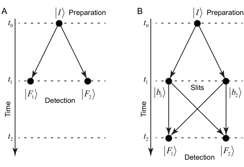
It is easy to recognize the setup as a rudimentary double-slit problem, where the states and play the role of two slits and and one of the two points on the screen, respectively (see Fig. 1B).
The expression in Eq.(1) is a particular combination of the amplitudes , defined for the four scenarios available to the system. The orthodox view of Section 2 is that such amplitudes are good only for calculating probabilities, defined as their (or their sum’s) absolute squares. Clearly, the complex valued weak value (1) is neither a probability, nor a conventional average. Could this be a chance to learn something Feynman’s orthodoxy has missed?
We note from the start that it is, however, unlikely. In essence, Feynman argues that one can always know the probability amplitudes, but is still unable to conclude whether the has system passed through one of the slits, or through both. Since the amplitudes are known, one can also know the expressions in the r.h.s. of Eq.(1). What could be special about them?
For one thing they can be measured in a laboratory [14]. However, Eq.(1) does not define a new way of calculating quantum mechanical averages. Rather, one measures the average position (reading) of the pointer in the standard manner, and uses this conventional average to work out, e.g., the real part of (see Appendix A). This is neither new, nor particularly unusual. Response of a quantum system to a small perturbation is always expressed in terms of the system’s amplitudes (see Appendix B for a simple example). If the weak values do describe new physics, as was suggested in [14], they must also have a truly new physical meaning. We will consider their possible interpretations after making sure that we, and the authors of [14], are indeed talking about the same thing.
6 A historical note
The history of weak values can be traced back to 1964 when the authors of [15] evaluated intermediate mean value of an operator for a system pre- and post-selected in the states and ,
| (2) | ||||
where , and . The Aharonov–Bergmann–Lebowitz rule [the first equality in (2)] is clearly an example of the Feynman’s rule for assigning probabilities [6] [the second equality in (2)] in the case where all scenarios can be distinguished. Indeed, it can be obtained as a mean reading of an accurate pointer, by using Eq.(LABEL:A2). Calculating the same average for a weakly coupled pointer, the authors of [14] obtained a somewhat similar expression,
| (3) | ||||
where is the coupling strength. (Noteworthy, a weak pointer, , , , is transformed into inaccurate one by a transformation , , , whereby . This would yield Eqs.(2) and (1) for the strong and weak regimes, respectively.) The quantities in the brackets are two equivalent forms of weak value , introduced earlier in Eq.(1) for .
7 Looking for the meaning of the weak values
To an orthodox this search is the most important endeavor of the whole saga. It is also the main purpose of this paper. A pre- and post-selected system, coupled to a pointer, is described by the transition amplitudes [see Eq.(17)], so whatever can be learned about the pointer will always be expressed in terms of these amplitudes. The weak value in Eq.(1) is a combination of amplitudes, and a kind of amplitude itself. Believing in the Uncertainty Principle, the orthodox also believes that knowing the amplitudes (which are always available) can provide no insight into how a particle goes through two slits, or, more generally, into a quantum system’s past. If the weak values are able to shed a new light on this vexed issue, Feynman’s warnings come to nothing, and the orthodox view of the theory does require a radical overhaul. But if they cannot do so, and Feynman was right, the weak measurements can lead one into the by now proverbial blind alley.
As yet there is little clarity as to the physical meaning of a weak value, although the real part can be written as a particular conditional expectation value [16]. Below we will question (without prejudice to practical utility of the weak measurement technique) several propositions which can be found in the literature. We will test them on the double slit problem in Fig. 1B, choosing the operator in Eqs.(1) and (3) to be a projector onto the first of the two states ,
| (4) |
7.1 A weak value represents the mean value of a variable with interference intact (?)
References [14], [17], come close to suggesting it, when it was argued that a negative kinetic energy can be attributed to a particle in a classically forbidden region. On the other hand, tunnelling is an interference phenomenon (see, e.g., [18]), and the orthodox view implies that the value of kinetic energy, like the slit chosen by the particle, must remain indeterminate. Indeed, measuring the accurate (strong) mean value of any is in itself a which way problem, as is seen from our double slit example. After trials, in which the system is always found in at , one counts the number of times, , the system takes the route , and evaluates a sum which agrees with (2) as . An accurate mean value of in (4) is, therefore, the conditional probability of taking the route passing via at , given that the system arrives in at .
A weak pointer does not distinguish between the two scenarios, and the number of times the route is taken is not only known, but, according to the Uncertainty Principle, cannot even be defined in a meaningful way. This given, something must go wrong with treating as a conditional probability, and it is easy to see what. The projector’s weak value
| (5) |
is an amplitude (renormalised, but still an amplitude) and may take complex values. One does not want to say that the system travels a route in out of cases, since it is not clear what it means. The real and imaginary parts of are also poor candidates for the role, since they can take either sign, and exceed unity. The modulus is, indeed, positive but may be too large (see Appendix C). In brief, in Eq.(5) cannot be used to determine the relative frequency with which a system, unobserved at , arrives in via the route . The same difficulty occurs with the weak value of a more general operator, .
The orthodox is not surprised. He knows that quantum amplitudes are not suited for making which way predictions, and does not expect a weak measurement to yield a further insight into the double slit conundrum.
7.2 The weak value of a projector is an occupation number (?)
This suggestion was made in [19] which analysed a four-slit problem with path amplitudes , and , and later in [14] dealing with a three-slit problem with . In both cases it was proposed that there can be negative number of particles, or particle pairs, passing through an arm of an interferometer.
The idea is also easily tried on the double slit problem. To avoid encountering even more mysterious complex occupation numbers one can make all the amplitudes in (26) real by putting . Now choosing , and following [14] and [19], one needs particles (copies of the system) in the path , and particles in the path . An explanation usually consists of describing a new phenomenon in terms of previously defined concepts. The above is a hardly an explanation of the double slit phenomenon, since the concept of having a negative number of particles is itself undefined.
For an orthodox the measured values and only reflect the correct relations between the amplitudes and , whilst the search for a deeper meaning of these numbers must end in a blind alley. And so it does. Explaining detection of the system in its final state as a result of a conspiracy between thousands of copies of the same system may seem a little too extravagant. Forget, therefore, numerical values. Perhaps the mere fact that a weak value does not vanish has a clearer meaning?
7.3 None-zero weak value of a projector indicates presence of the system at the chosen location (?)
It does, say the authors of [5]. So much so, that a system and its particular property can part company and go their different ways. One, for example, can separate […] internal energy of an atom from the atom itself [5]. For the double slit example a similar proposition means that whenever neither amplitude vanishes, the particle goes through both slits at once. However, according to [9], this directly contradicts the Uncertainty Principle, as well as the experimental evidence, since wherever one looks, he finds either entire system, or nothing.
The orthodox may also add that, as in the case of the Bohmian particle, there is a problem with locality. A final state can be reached via two paths (arms of the interferometer in an optical realization of the experiment), each endowed with an amplitude , . A property, local to the first arm, can be expected to depend only on one amplitude, , and not on what happens in the other parts of the setup. After trials, the experimenter counts the number of times, , the system is found in and the pointer’s reading lies in an interval around . He can calculate a kind of average reading
| (6) |
(It would be more natural to calculate the conditional average by dividing by the number of successful post-selections in . This would yield Eqs.(2) and (1) for the strong and weak regimes, respectively. However, the choice made in Eq.6 is more convenient for the point we are trying to make.)
In the accurate strong limit one has [cf. Appendix A]
| (7) |
clearly a local quantity which depends only on the amplitude of the route passing through the state , upon which projects. In the inaccurate weak limit the result
| (8) | ||||
is non-local in the above sense, due to the presence of the second amplitude . An attempt to probe the system locally while perturbing it only slightly, ends up probing all the pathways, leading to the same final condition. The orthodox may expect this from the Uncertainty Principle [6, 9]. There is, however, still one possibility left.
7.4 Null weak value of a projector indicates absence of the system from the chosen location (?)
Finally, this seems to be a safe option (for more discussion see [20]), since in Eq.(5) can vanish only if the amplitude is itself zero. With only one path, , leading to the final state, there is no interference to destroy. The strong and the weak measurements apparently agree in that the system never travels the route . However, there is still a problem. To discuss it we will have to leave the double slit case, and increase the number of routes, leading to the final state, to at least three.
8 A conjuring trick
Consider next a system in a three-dimensional Hilbert space, , pre- and post-selected as before in states and , respectively. Three projectors,
| (9) | |||
monitor the presence of the system in the paths , , as well as in their union. The states , and are chosen to ensure that one has
| (10) | |||
The accurate strong mean values of the three projectors, measured together, are [cf. Eq.(2)]
| (11) | |||
This agrees with one’s understanding of the concept of absence. If a system (or at least a given property of that system) is absent from the union of two paths, , it is because the system never takes either of them, , and .
However, using Eq.(1), for the weak values one finds [cf. Eq.(3)]
| (12) | |||
Unlike Eqs.(11), Eqs.(12) do not make conventional sense if the criterion (D) of the previous section is, indeed, valid. The system, not absent from the parts (since ) is nevertheless absent from the whole (since =0). How can it be? At this point the reader is expected to choose.
One option is to see this as a paradox peculiar to the bizarre quantum world. (In the same vein, by choosing in (12) , one can claim that a particle can be found with certainty in two different boxes [21], or that photons have discontinuous trajectories [22])
The other view is that there is no paradox, since the proposition (D) is simply wrong, and could, indeed, be expected to fail. One can only learn about the past scenario by destroying interference where various scenarios interfere. A weak pointer does not destroy it and, therefore, ceases to be a valid measuring device. Equations (12) only reflect the correct relations between the three amplitudes in Eq.(10), already known from the moment the choice (10) was made. There is no way around the Uncertainty Principle.
Our main point is that the second view must be the right one. To an orthodox the first option is an obvious fallacy. A proposition, based on a well defined concept, is found to contradict the evidence, the concept is amplified to encompass the evidence, so that the evidence can be seen as supporting the proposition. A meaningful explanation, or interpretation, is possible only if the standards against which a phenomenon is judged are maintained the same throughout the analysis. What is wrong is that we do not ask what is right [23]. The need to constantly change the basic concepts in order to suit particular views, is yet another kind of trouble one finds inside Feynman’s blind alley.
9 Summary
In a nutshell, the orthodox view expressed in [6, 24, 9] can be summarized as follows. The theorist’s task is to combine known probability amplitudes as appropriate, so that the absolute square of the result would yeld the desired probability. (Needless to say, his/her other task involves constructing, in each case, a Hilbert space, a Hamiltonian, and the operators, which represent the measured quantities.) This simple prescription, however, conceals a paradox [9], or a mystery [6]. The knowledge of the amplitudes alone cannot be used to determine a quantum system’s past. This is one way to state the Uncertainty Principle [6]. Feynman recommended adjusting one’s feelings about reality to reality, and strongly advised against rationalizing the quantum law using classical analogies. An often cited Feynman’s quote reads:
The ‘paradox’ is only a conflict between reality and your feeling of what reality ‘ought to be.’ [25, §18-3]
What may happen if this advice is ignored was illustrated by the three-slit case of Section 8. Accepting the premise that a vanishing amplitude signals the absence of the system from a path (or a box [21]), may lead to a paradoxical notion that a quantum system may be present in the parts, yet absent from the whole. To an orthodox, there is no paradox, but rather a proof that the premise was wrong.
This example underlines the main difficulty in finding a physical meaning for weak values in Eqs.(1), given by combinations of the relative (i.e., normalised to a unit sum over the paths connecting the initial and final states) probability amplitudes. Like the amplitudes themselves, these combinations are always known to the theorist, and the fact that their values can be deduced from the experimental data makes little difference to him. The question is whether weak values can consistently describe the system’s past in the presence of interference, something apparently forbidden by the Uncertainty Principle. The orthodox believes that such a description is not possible, and the few propositions studied in Section 7 appear to support this conclusion. If asked what is a ‘weak value’? he can only refer to the probability amplitudes which quantum theory uses to describe the measured system, and cite the Uncertainty Principle as the main limitation on their possible use.
Finally, the reader may ask whether all this nitpicking was really necessary. Surely the weak measurements have practical uses, e.g., due to their amplifying effect [14], so why deprive them of their allure? Why not allow for a bit of magic where it helps to advertise the approach, or to gain a publication in a prestigious journal? One answer is that, given the current interest in quantum technologies (some call it the second quantum revolution [26]), it is highly desirable to have full understanding of both possibilities and limitations of the basic theory which underpins the engineering developments.
Acknowledgment
The author gratefully acknowledges financial support from Grant PID2021-126273NB-I00 funded by MICINN/AEI/10.13039/501100011033 and by “ERDF A way of making Europe,” and from the Basque Government Grant No. IT1470-22.
10 Appendix A. Measurements, strong and weak
10.1 Two-step measurement
For our purpose it is sufficient to consider a system in a Hilbert space of a finite dimension . The simplest measurement consists of preparing it in a state (step one) and measuring an operator , diagonal in an orthonormal basis , , after time (step two). According to [6], there are scenarios, , amplitudes, [ is the system’s evolution operator] (see Fig. 1A). There are also probabilities, , since all the scenarios lead to distinguishable final conditions [6]. One can couple to the system a von Neumann pointer [27] with position , prepared in a state . The coupling Hamiltonian is , and is a real valued smooth function, peaked around , with a characteristic width and zero mean,
| (13) |
In each of the above scenarios the pointer’s state is displaced by . Thus, the probability to find a pointer’s reading is simply
| (14) |
The mean reading,
| (15) | ||||
is, therefore, independent of the initial uncertainty in the pointer’s position, , which determines the accuracy of the measurement. This, we note, is because all system’s scenarios are a priori endowed with probabilities, and there is no interference the pointer can destroy. This changes if more measurements are made.
10.2 Three-step measurement
Interesting interference effects first appear if the previously prepared system is to be measured twice, at in a basis , and then at in a basis . There are scenarios, , and amplitudes,
| (16) | ||||
If the system is left on its own, the scenarios interfere, and individual probabilities can be assigned only if this interference is destroyed [6]. The measurement at accurately determines the system’s final state , but at the measurement of an operator can be fuzzy, . It each scenario the pointer’s state is shifted by , and the transition amplitudes of the composite {system + pointer} are particularly simple,
| (17) |
Now the joint probability of finding the system in at , and having a pointer’s reading , is given by
| (18) |
which reduces to in Eq.(14) if summed over all final states,
| (19) |
i.e., if the information about the measurement at is erased. The exact form of now depends on how accurately is measured. A highly accurate strong measurement, , destroys the interference,
and finding the experimenter knows that the system has traveled the route . The mean reading, conditional on the system arriving in , is, therefore, given by [cf. Eq.(2)]
| (21) |
In the opposite inaccurate weak limit, , is broad in , interference is not destroyed, and an individual reading cannot identify the route taken by the system.
The role of the Uncertainty Principle [6] is best illustrated by treating the states and as the slits, and the points on the screen, respectively. Now is the observed intensity, which contains an inteference pattern, provided
| (22) | |||
In the weak limit one can still evaluate , and using finds
Measuring the pointer’s mean momentum, , allows one to determine its imaginary part (see, e.g., [28])
| (24) |
where , and .
After two experiments, each involving many trials, the experimenter determines the value of a complex quantity . It is up to the theorist to explain what exactly has been learned about the observed system.
11 Appendix B. Response of a system to a small perturbation
A two-level system is making a transition between states and . The probability to detect it in after a time is . A small perturbation , introduced at , changes the transition amplitude to , with The probability of detection then changes to , where . From the measured percentage change in the detection probability one can deduce the imaginary part of the weak value of the perturbation [cf. Eq.(1)],
| (25) |
12 Appendix C. Transition amplitudes for a two-level system in Fig. 1B
Without loss of generality, we choose the initial state of the spin to be polarized along the -axis, , the states at to be polarized along a direction , , and the final states polarized up and down an axis , . System’s evolution, if any, can be absorbed in the states and , so we also choose . The four amplitudes are
| (26) | |||
Adding them up yields the two amplitudes in Fig. 1A,
| (27) | |||
For and , the weak value of the projector in Eq.(4) is complex valued, with no restriction on the signs of its real and imaginary parts,
| (28) |
For , and , becomes a dark state (akin to a dark fringe in the interference pattern). The weak value tends to
| (29) |
and can exceed unity. For example, putting , , yields ()
| (30) |
References
- [1] D. Sokolovski. Are the weak measurements really measurements?. Quanta 2013; 2:50–57. doi:10.12743/quanta.v2i1.15.
- [2] Y. Aharonov, E. Cohen, A. Landau, A. C. Elitzur. The case of the disappearing (and re-appearing) particle. Scientific Reports 2017; 7(1):531. doi:10.1038/s41598-017-00274-w.
- [3] Y. Aharonov, E. Cohen, S. Popescu. A dynamical quantum Cheshire Cat effect and implications for counterfactual communication. Nature Communications 2021; 12(1):4770. doi:10.1038/s41467-021-24933-9.
- [4] C. Ferrie, J. Combes. How the result of a single coin toss can turn out to be heads. Physical Review Letters 2014; 113(12):120404. doi:10.1103/PhysRevLett.113.120404.
- [5] Y. Aharonov, S. Popescu, D. Rohrlich, P. Skrzypczyk. Quantum Cheshire Cats. New Journal of Physics 2013; 15(11):113015. doi:10.1088/1367-2630/15/11/113015.
- [6] R. P. Feynman, R. B. Leighton, M. L. Sands. Quantum behavior. in: The Feynman Lectures on Physics. Volume III. Quantum Mechanics. California Institute of Technology, Pasadena, California, 2013. https://www.feynmanlectures.caltech.edu/III_01.html.
- [7] G. K. Chesterton. Heretics. John Lane, London, 1905. https://archive.org/details/heretics01chesgoog.
- [8] R. P. Feynman. Epaulettes and the Pope. in: The Pleasure of Finding Things Out. Perseus Books, Cambridge, Massachusetts, 1999. pp. 7–8.
- [9] R. P. Feynman. The Character of Physical Law. MIT Press, Cambridge, Massachusetts, 1985.
- [10] N. D. Mermin. Hidden variables and the two theorems of John Bell. Reviews of Modern Physics 1993; 65(3):803–815. doi:10.1103/RevModPhys.65.803.
- [11] J. Faye. Copenhagen interpretation of quantum mechanics. in: E. N. Zalta (Ed.), Stanford Encyclopedia of Philosophy. Stanford University, Stanford, California, 2019. https://plato.stanford.edu/entries/qm-copenhagen/.
- [12] S. Goldstein. Bohmian mechanics. in: E. N. Zalta (Ed.), Stanford Encyclopedia of Philosophy. Stanford University, Stanford, California, 2021. https://plato.stanford.edu/entries/qm-bohm/.
- [13] D. Sokolovski, D. Alonso Ramirez, S. Brouard Martin. Speakable and unspeakable in quantum measurements. Annalen der Physik 2023; 535(10):2300261. doi:10.1002/andp.202300261.
- [14] Y. Aharonov, S. Popescu, J. Tollaksen. A time-symmetric formulation of quantum mechanics. Physics Today 2010; 63(11):27–32. doi:10.1063/1.3518209.
- [15] Y. Aharonov, P. G. Bergmann, J. L. Lebowitz. Time symmetry in the quantum process of measurement. Physical Review 1964; 134(6B):B1410–B1416. doi:10.1103/PhysRev.134.B1410.
- [16] A. Matzkin. Weak values and quantum properties. Foundations of Physics 2019; 49(3):298–316. doi:10.1007/s10701-019-00245-3.
- [17] Y. Aharonov, S. Popescu, D. Rohrlich, L. Vaidman. Measurements, errors, and negative kinetic energy. Physical Review A 1993; 48(6):4084–4090. doi:10.1103/PhysRevA.48.4084.
- [18] X. G. de la Cal, M. Pons, D. Sokolovski. Speed-up and slow-down of a quantum particle. Scientific Reports 2022; 12(1):3842. doi:10.1038/s41598-022-07599-1.
- [19] Y. Aharonov, A. Botero, S. Popescu, B. Reznik, J. Tollaksen. Revisiting Hardy’s paradox: counterfactual statements, real measurements, entanglement and weak values. Physics Letters A 2002; 301(3):130–138. doi:10.1016/S0375-9601(02)00986-6.
- [20] Q. Duprey, A. Matzkin. Null weak values and the past of a quantum particle. Physical Review A 2017; 95(3):032110. doi:10.1103/PhysRevA.95.032110.
- [21] T. Ravon, L. Vaidman. The three-box paradox revisited. Journal of Physics A: Mathematical and Theoretical 2007; 40(11):2873–2882. doi:10.1088/1751-8113/40/11/021.
- [22] A. Danan, D. Farfurnik, S. Bar-Ad, L. Vaidman. Asking photons where they have been. Physical Review Letters 2013; 111(24):240402. doi:10.1103/PhysRevLett.111.240402.
- [23] G. K. Chesterton. What’s Wrong with the World. Cassell and Company, London, 1910. https://archive.org/details/whatswrongwithwo03chesuoft.
- [24] R. P. Feynman, A. R. Hibbs. Quantum Mechanics and Path Integrals. McGraw-Hill, New York, 1965.
- [25] R. P. Feynman, R. B. Leighton, M. L. Sands. Angular momentum. in: The Feynman Lectures on Physics. Volume III. Quantum Mechanics. California Institute of Technology, Pasadena, California, 2013. https://www.feynmanlectures.caltech.edu/III_18.html.
- [26] J. P. Dowling, G. J. Milburn. Quantum technology: the second quantum revolution. Philosophical Transactions of the Royal Society of London Series A: Mathematical, Physical and Engineering Sciences 2003; 361(1809):1655–1674. doi:10.1098/rsta.2003.1227.
- [27] J. von Neumann. Mathematical Foundations of Quantum Mechanics. Princeton University Press, Princeton, 1955. doi:10.23943/princeton/9780691178561.001.0001.
- [28] D. Sokolovski. Weak measurements measure probability amplitudes (and very little else). Physics Letters A 2016; 380(18-19):1593–1599. doi:10.1016/j.physleta.2016.02.051.