Exploiting Automorphisms of Temporal Graphs for Fast Exploration and Rendezvous

Abstract

Temporal graphs are dynamic graphs where the edge set can change in each time step, while the vertex set stays the same. Exploration of temporal graphs whose snapshot in each time step is a connected graph, called connected temporal graphs, has been widely studied. In this paper, we extend the concept of graph automorphisms from static graphs to temporal graphs for the first time and show that symmetries enable faster exploration: We prove that a connected temporal graph with $n$ vertices and orbit number $r$ (i.e., $r$ is the number of automorphism orbits) can be explored in $O(rn^{1+\epsilon})$ time steps, for any fixed $\epsilon>0$. For $r=O(n^{c})$ for constant $c<1$, this is a significant improvement over the known tight worst-case bound of $\Theta(n^{2})$ time steps for arbitrary connected temporal graphs. We also give two lower bounds for temporal exploration, showing that $\Omega(n\log n)$ time steps are required for some inputs with $r=O(1)$ and that $\Omega(rn)$ time steps are required for some inputs for any $r$ with $1\leq r\leq n$.

Moreover, we show that the techniques we develop for fast exploration can be used to derive the following result for rendezvous: Two agents with different programs and without communication ability are placed by an adversary at arbitrary vertices and given full information about the connected temporal graph, except that they do not have consistent vertex labels. Then the two agents can meet at a common vertex after $O(n^{1+\epsilon})$ time steps, for any constant $\epsilon>0$. For some connected temporal graphs with the orbit number being a constant, we also present a complementary lower bound of $\Omega(n\log n)$ time steps.

1 Introduction

For many decades, graph theory has been a tool used to model and study many real world problems and phenomena [16]. A usual assumption for many of these problems is that the graphs have a fixed structure. However, there are quite a number of cases where the structure of a system changes over time. For example, consider the problem of routing in transportation networks (roads, rails) where specific connections can become unavailable (due to a disaster) or they are active during specific times (due to safety). Such scenarios can be modeled using temporal graphs, a sequence of graphs over the same vertex set where the edges possibly change in each time step. The temporal graph setting has received significant interest from the research community in the recent past as seen in recent surveys [19, 46].

In this paper, we study two problems on temporal graphs. The first is the temporal exploration problem (texp), which has been studied, e.g., by Michail and Spirakis [47, 48] and by Ilcinkas et al. [35]. It requires an agent to explore all vertices of the temporal graph as quickly as possible. The second is the temporal rendezvous problem (trp), which we formulate for the first time in this paper. It requires two heterogeneous agents (in terms of the programs they run) to rendezvous on a temporal graph when they cannot communicate with one another. For both problems, we assume that each agent has complete knowledge of the temporal graph in advance (a common assumption [3, 15, 26, 27, 28, 29, 35, 47, 48, 60]). However, in the case of trp the agents may have different names for the same vertices, i.e., the local labels of the vertices may be different.

The problem of exploration has been well studied in the static setting since it was introduced in 1951 by Shannon [57]. It has also been intensively studied in the temporal graph setting since 2014 (see all references from the last paragraph). On an application-oriented note, the problem captures the setting where a person is trying to visit various parts of a city using changing public transportation. For example, train schedules involve multiple train stations (vertices) with trains running between them at different times (i.e., repeatedly changing edges). Thus, planning a visit to multiple destinations over a given day using railways is an example of solving texp.

The rendezvous problem can be broadly categorized into two types: symmetric and asymmetric rendezvous. The version where agents have the same strategy (symmetric rendezvous) was introduced by Alpern [11]. The version where agents can have distinct strategies (asymmetric rendezvous) was introduced by Alpern [8] and is the focus of research in this paper. trp is a natural extension of the asymmetric rendezvous problem to the dynamic setting. As a real world example, consider a pair of tourists who want to explore a city together and have to agree on a strategy to meet up in case they are separated and their cell phones die. In this scenario, they may use public transportation (dynamically changing network) to meet and agree in advance to use different strategies that guarantee that they meet quickly.

In this paper, we present results that extend the literature in two ways. Firstly, we formalize the trp problem in the setting where agents have complete knowledge of the temporal graph a priori and develop good upper and lower bounds for it. Secondly, we utilize interesting structural properties (namely automorphisms of a graph and associated orbits of vertices) in order to analyze bounds on the number of time steps required by temporal walks that solve certain problems. In particular, we develop upper and lower bounds for both texp and trp that leverage the aforementioned graph properties. To the best of our knowledge, this is the first work that takes advantage of these graph properties to study problems in temporal graphs.

1.1 Our Contributions

We present results for two problems: first, the temporal exploration problem (texp) which, for a given temporal graph $\mathcal{G}$, asks for a temporal walk that visits all vertices of $\mathcal{G}$, and secondly, the temporal rendezvous problem (trp), which considers two agents that try to meet in the given temporal graph, meaning they must be stationed at the same vertex in the same time step.

One of our primary contributions is formalizing the problem of trp in Section 2, and in doing so extending the problem of asymmetric rendezvous to the temporal graph setting where agents have complete knowledge of the temporal graph in advance. Another significant contribution is that we show how to leverage the use of a structural graph property, namely the automorphism group (with function composition as group operation) of a temporal graph and the associated notion of orbits, to bound the number of time steps required by algorithms we devise for these problems. To the best of our knowledge, this work is the first instance of leveraging such properties to study any problem on temporal graphs. Intuitively, an automorphism of a graph is a mapping from the set of vertices of the graph to the same set of vertices that preserves the neighborhood relation between the vertices. The set of automorphisms of a temporal graph consists of the intersection of the sets of automorphisms of the graph at each time step. The set of automorphisms of the temporal graph, along with function composition as group operation, forms the automorphism group of the temporal graph. An orbit of the automorphism group of a temporal graph is a maximal set of vertices such that each vertex can be mapped to any other vertex in the set via an automorphism of the group. Intuitively, the vertices in an orbit look indistinguishable to an agent that has full information about the temporal graph but without meaningful vertex labels. Under the assumption that the agents are able to compute the orbits (Lemma 5.1) two agents can agree to meet in some specific orbit, but not at a specific vertex. Therefore, temporal graphs where all orbits are large (or that even have a single orbit containing all vertices) appear to be the most challenging graphs for solving trp. Our result providing fast exploration schedules in temporal graphs with few orbits is therefore a crucial ingredient for enabling our solution to trp to handle all possible temporal graphs (including those with a single orbit).

We give precise definitions and present further preliminaries in Section 2. Then, we introduce some useful utilities related to automorphisms in Section 3. These will be used in later sections, where we present the following results.

Upper bounds. In Section 4, we develop a deterministic algorithm to solve texp in $O(rn^{1+\epsilon})$ time steps for any fixed $\epsilon>0$ (see Corollary 4.15), where $n$ is the number of vertices in the temporal graph and $r$ is the number of orbits of the automorphism group of the temporal graph. Note that $r$ can range in value from $1$ to $n$. Thus, for $r=O(n^{c})$ for constant $c<1$, this is a significant improvement over the known tight worst-case bound of $\Theta(n^{2})$ time steps for arbitrary connected temporal graphs [26]. In Section 5, we leverage this algorithm for texp to develop a deterministic solution for trp using $O(n^{1+\epsilon})$ time steps for any fixed $\epsilon>0$ (see Theorem 5.3). Note that our focus is on bounding the time steps of the temporal walks required to solve texp and trp, and not on optimizing the running time of the respective algorithms to compute such walks.

Lower bounds. We complement our algorithms with lower bounds for both texp and trp in Section 6. In particular, we design an instance of trp such that any solution for it requires $\Omega(n\log n)$ time steps (see Theorem 6.3). We then show how this translates to a lower bound of $\Omega(n\log n)$ time steps for some instances of texp where the temporal graph at hand has an orbit number $r=O(1)$ (see Corollary 6.5). By revisiting the lower bound of [26] for texp, which focused on arbitrary temporal graphs, and studying it through the lens of automorphisms and orbits, we can obtain a more fine-grained lower bound of $\Omega(rn)$ time steps (see Lemma 6.1) for some temporal graphs with orbit number $1\leq r\leq n$. Notice that the multiplicative gap between our upper and lower bounds for both problems is only a factor of $O(n^{\epsilon})$.

Relevance of the orbit number. It is well known in graph theory that almost all (static) graphs are rigid [13], meaning that the automorphism group contains only the trivial identify function. This is in contrast to observations in practice. Many real-world graphs have non-trivial automorphisms. A recent analysis of real-world graphs in the popular database networkrepository.com showed that over $70\%$ of the analyzed graphs had non-trivial automorphisms [13]. One may reasonably expect that real-world temporal graphs have similar properties. Symmetries are also abundant in graphs arising in chemistry [12], which have been studied in temporal settings as well [55]. We believe that these observations provide a strong motivation for studying temporal graph problems for temporal graphs with fewer than $n$ orbits, e.g., with algorithms parameterized via the number of orbits. Furthermore, we emphasize that our results for trp hold for all temporal graphs, independent of the orbit number parameter, even though they utilize techniques we develop for texp parameterized by the orbit number. Roughly speaking, for orbit number $r$, the penalty factor $r$ in the number of time steps to solve texp is saved when solving trp by focusing only on a smallest orbit of size at most $n/r$.

1.2 Technical Overview and Challenges

Firstly, we give an intuitive overview of our upper bound results. The concepts used in this section are more precisely defined in the next sections.

For texp, we first consider the problem of visiting all the vertices of one orbit $S$. One key insight is that, if we have a temporal walk $W$ that visits $k$ vertices of $S$, we can use the automorphisms of the temporal graph to transform $W$ into other walks that visit different sets of $k$ vertices of $S$ (Lemma 3.3). Therefore, even if the $k$ vertices visited by $W$ have already been explored earlier, we can transform $W$ into a temporal walk $W^{\prime}$ that visits a “good” number of previously unexplored vertices of $S$. The number of previously unexplored vertices of $S$ that $W^{\prime}$ is guaranteed to visit increases with the number of possible start vertices in $S$ that we allow for $W^{\prime}$, but the larger that set $X$ of possible start vertices is, the longer it may take the agent to reach the best start vertex in that set. A challenge is to analyze this tradeoff. By carefully relating the size of $X$ to the guaranteed number of unexplored vertices that a walk $W^{\prime}$ starting at a vertex in $X$ can visit (Corollary 3.5), we manage to balance the number of time steps needed to move to the start vertex of $W^{\prime}$ and the number of previously unexplored vertices that $W^{\prime}$ visits. To show that vertices of $S$ can be reached quickly, we study the structure of edges that connect vertices in different orbits (Lemma 4.1) and use it to analyze reachability between orbits (Lemmas 4.3 and 4.5).

We then employ a recursive construction: We recursively construct a temporal walk $W_{1}$ that visits $k$ vertices of $S$, concatenate $W_{1}$ with a temporal walk that moves quickly from the endpoint of $W_{1}$ to a good start vertex in $S$ for the second recursively constructed walk, and then use a second recursively constructed walk (transformed via an automorphism to a “good” temporal walk $W_{2}$ starting in a vertex of $S$) to visit “nearly” $k$ further vertices of $S$. A careful analysis then shows that in this way we can visit a constant fraction of the vertices of $S$ in $O(r|S|^{1+\epsilon})$ steps (Lemma 4.9 and Corollary 4.11). We then show that the concatenation of $O(\log|S|)$ such walks (each one again transformed via an automorphism to maximize the number of newly explored vertices) suffices to visit all vertices of $S$ in $O(r|S|^{1+\epsilon}+n\log|S|)$ time steps (Theorem 4.13), which can be bounded by $O(rn^{1+\epsilon^{\prime}})$ time steps). By visiting the $r$ orbits one after another, we can finally show that the whole temporal graph can be explored in $O(rn^{1+\epsilon^{\prime}})$ time steps (Corollary 4.15).

For trp, a simple and fast solution one first thinks of is to have the agents simply meet at a vertex with a specific label. However, this is not feasible in the model we consider. In particular, we assume that the agents cannot communicate and, while both agents have complete information about the temporal graph, they do not have access to consistent vertex labels. As such, the agents are unable to agree upon the same vertex based on the vertex label. We rely, instead, on structural graph properties and let the agents meet at a vertex in a smallest orbit: One agent moves to any vertex in that orbit, and the other searches all vertices in that orbit. The first challenge is for the agents to independently identify the same orbit in which to meet. We show that this can be done by letting each agent enumerate all temporal graphs, together with colorings of their orbits, until it encounters for the first time a temporal graph that is isomorphic to the input graph in which trp is to be solved. In this way both agents obtain the same colored temporal graph and can independently select, among all orbits of smallest size, the one with smallest color (Lemma 5.1). Then one agent moves to a vertex in that orbit $S$, while the other searches all vertices of $S$. The challenge here is to deal with orbits that are large, because previously known techniques would require $\Theta(n^{2})$ time steps to explore an orbit of size $\Omega(n)$. Fortunately, this is where our above-mentioned results for exploration of (orbits of) temporal graphs come to the rescue: As $|S|\leq n/r$, we have $O(r|S|^{1+\epsilon}+n\log|S|)=O(n^{1+\epsilon^{\prime}})$, and hence $S$ can be explored (and trp solved) in $O(n^{1+\epsilon^{\prime}})$ time steps (Theorem 5.3).

Now we turn to our lower bounds. For texp, we first observe that the existing lower bound construction that shows that $\Omega(n^{2})$ time steps are necessary for exploration on some temporal graphs uses temporal graphs with $\frac{n}{2}+1$ orbits. By slightly varying the construction, we can show for any $r$ in the range from $1$ to $n$ that there are temporal graphs with $r$ orbits that require $\Omega(rn)$ time steps for exploration (Lemma 6.1). Our main lower bound result is the lower bound of $\Omega(n\log n)$ for trp in temporal graphs with a single orbit (Theorem 6.3). The temporal graph is a cycle on $n=2^{m}-1$ vertices in every step, and the edges change every $\lfloor n/16\rfloor$ time steps. Each period of $\lfloor n/16\rfloor$ time steps in which the edges do not change is called a phase. We number the vertices of the cycle from $0$ to $n-1$ and consider the binary representation of the vertex labels. In phase $1$, each vertex $j$ is adjacent to $j+1$ and $j-1$, while in any phase $i>1$, it is adjacent to $j+2^{2i}$ and $j-2^{2i}$ (with all computations done modulo $n$). As all vertices are indistinguishable to the agents, we can force each agent to make the same movements no matter where we place it initially. By fixing the five highest-order bits of the agents’ start positions in a certain way, we can ensure that the agents do not meet in the first phase, no matter how the remaining bits of their start positions are chosen. Depending on the positions where the agents end up at the end of each phase (relative to their start position in that phase), we fix a certain number of bits of the binary representations of the start positions of the agents: After the first phase, we fix the lowest four bits, and after each further phase, we fix the next-higher two bits. We can show that this is sufficient to ensure that the agents start the next phase at vertices that are sufficiently far from each other in the cycle of that phase. This process can be repeated $\Omega(\log n)$ times, showing that it takes $\Omega(n\log n)$ time steps for the agents to meet. This lower bound for trp implies also that exploration of the constructed temporal graph requires $\Omega(n\log n)$ steps (Corollary 6.5).

1.3 Related Work

There is a divide in the research on temporal graphs with respect to the amount of knowledge known in advance by the agents on the graph. When complete knowledge of the temporal graph is known in advance to the agents, as is assumed in this paper, the setting is sometimes referred to as the post-mortem setting (see, e.g., Santoro [56]). Since we consider scenarios were agents plan temporal walks using advance knowledge of future time steps, we refer to the post-mortem setting as the clairvoyant setting in the remainder of this section.

The clairvoyant setting is in contrast to the live setting where agents only have partial knowledge of the temporal graph, and the solutions to problems in these different settings are of a different nature. The reader can refer to the survey by Di Luna [22] for more information on problems and solutions in the live setting. We restrict the rest of this related work section to work in the clairvoyant setting.

Exploration. We trace the progress of solving instances of texp, first by identifying which assumptions are required for the problem to even be solvable, and then by identifying properties that were leveraged to give faster and faster solutions.

Michail and Spirakis [47, 48] showed that it is NP-complete to decide whether a given temporal graph with a given lifetime, i.e., the number of time steps it exists, is explorable when no assumptions are made on the input graph. This holds even if the graph is connected in every time step, termed connected (and sometimes called always-connected in the literature). Even when a restriction is placed on the underlying graph, i.e., the union of the graphs at each time step, such that the underlying graph has pathwidth at most $2$, Bodlaender and van der Zanden [15] showed that texp is NP-complete.

However, the exploration is always possible when the lifetime of the graph is sufficiently large. In particular, Michail and Spirakis [48] showed that a connected graph with $n$ vertices may be explored in $O(n^{2})$ time steps. For the rest of the related work on texp, we focus on the case of connected temporal graphs with a sufficiently large lifetime. Erlebach et al. [26] showed that exploration on arbitrary temporal graphs takes $\Omega(n^{2})$ time steps. By restricting their study of temporal graphs to those where the underlying graph belongs to a special graph class, however, they showed that texp can be solved in $o(n^{2})$ time steps in several such cases. In particular, when the underlying graph is planar, has bounded treewidth $k$, or is a $2\times n$ grid, they showed that texp can be solved in $O(n^{1.8}\log n)$ time steps, $O(n^{1.5}k^{1.5}\log n)$ time steps, and $O(n\log^{3}n)$ time steps, respectively. They also showed a lower bound of $\Omega(n\log n)$ when the underlying graph is a planar graph of degree at most $4$.

The study of texp when the temporal graph is restricted continued in several papers. Taghian Alamouti [60] showed that texp can be solved in $O(k^{2}(k!)(2e)^{k}n)$ time steps when the underlying graph is a cycle with $k$ chords. Adamson et al. [3] improved this to $O(kn)$ time steps. They also improved the upper bounds on texp for underlying graphs that have bounded treewidth $k$ or are planar to $O(kn^{1.5}\log n)$ and $O(n^{1.75}\log n)$, respectively. In addition, they strengthened the lower bound for underlying planar graphs by showing that even if the degree is at most $3$, the lower bound is $\Omega(n\log n)$. Erlebach et al. [27] further improved work on bounded degree underlying graphs by showing that texp can be solved in $O(n^{1.75})$ time steps for such temporal graphs. Ilcinkas et al. [35] showed that when the underlying graph is a cactus, the exploration time is $2^{\Theta(\sqrt{\log n})}n$ time steps.

Other variants of texp have been studied where the problem is slightly different, or the edges of the temporal graph vary in some particular way (e.g., periodically, $T$-interval connected, $k$-edge deficient), or multiple agents explore the graph [1, 2, 5, 18, 28, 29, 36].

Rendezvous. Symmetric rendezvous [11] and asymmetric rendezvous  [8] have received much interest over the years, resulting in numerous surveys [9, 10, 30, 38, 39, 52, 53] being written on the problems covering different settings. In this work, we are the first to extend asymmetric rendezvous to temporal graphs in the clairvoyant setting. Note that there has been previous work [17, 21, 23, 49, 51, 58, 59] that has studied multi-agent rendezvous (also called gathering) in a dynamic graph setting, but that was in the live setting. For an overview of rendezvous in static graphs we refer the reader to [7, 39]. Rendezvous has been studied in deterministic settings [14, 54] and asynchronous settings [24, 41], and has been shown to be solvable in logarithmic space [20].

Other Related Work. Other problems have also been studied in the temporal graph setting, e.g., matchings [44], separators [32, 61], vertex covers [6, 34], containments of epidemics [25], Eulerian tours [18, 42], graph coloring [43, 45], network flow [4], treewidth [31] and cops and robbers [50]. See the survey by Michail [46] for more information.

2 Preliminaries

Basic terminology. We use standard graph terminology. All static graphs are assumed to be simple and undirected. We write $[x]=\{1,\ldots,x\}$ for any integer $x$.

A temporal graph $\mathcal{G}=(G_{1},\ldots,G_{\ell})$ is a sequence of static graphs, all with the same vertex set $V$. For a temporal graph $\mathcal{G}$, the graph $G=(V,\bigcup_{t\in[\ell]}E(G_{t}))$ is the underlying graph of $\mathcal{G}$. We call $\mathcal{G}$ connected if each $G_{t}$ for $t\in[\ell]$ is connected. We use $n$ to refer to the number of vertices of the (temporal) graph under consideration. A temporal walk $W$ is a walk in a temporal graph $\mathcal{G}$ that is time respecting, i.e., traverses edges in strictly increasing time steps. For a temporal walk $W$ starting at time step $t$ we write $W=(u_{1},u_{2},u_{3},\ldots)$ to mean the temporal walk starts at vertex $u_{1}$ in time step $t$, is at vertex $u_{2}$ at the beginning of time step $t+1$, and so forth. Note that subsequent vertices in the temporal walk can be the same vertex, i.e., we can wait for an arbitrary number of time steps at a vertex. We say that a temporal walk spans $x$ time steps if it starts at some time step $t$ and ends at some time step $t^{\prime}$ with $t^{\prime}-t=x$. We assume that the lifetime $\ell$ is large enough such that a desired temporal walk can be constructed. For all our results it is enough to assume $\ell\geq n^{2}$, as $n^{2}$ time steps suffice for texp [26] and therefore also for trp. For any function $f:X\rightarrow X$ for a universe $X$ we write $f^{i}(x)$ when we mean applying the function $i$-times iteratively for any $x\in X$ and integer $i$, e.g., $f^{2}(x)=f(f(x))$. We use $\circ$ to denote function composition, i.e., for two functions $f:X\rightarrow X$ and $g:X\rightarrow X$, we denote with $f\circ g$ the function that maps $x\in X$ to $f(g(x))$.

Isomorphisms and automorphisms. Two static graphs $G$ and $H$ are isomorphic exactly if a bijection $\theta:V(G)\rightarrow V(H)$ (called an isomorphism) exists with the following property: two vertices $u,v$ are adjacent in $G$ exactly if $\theta(u)$ is adjacent to $\theta(v)$ in $H$. We write $G\cong H$ if $G$ is isomorphic to $H$. An automorphism is an isomorphism from a graph $G$ to itself. The set of all automorphisms of a graph $G$ forms a group $\text{Aut}(G)$, with $\circ$ as group operation. Refer to [33, 37, 40] for further reading on the topic of isomorphisms and automorphisms of graphs.

For a temporal graph $\mathcal{G}$ with lifetime $\ell$ we denote with $\text{Aut}(\mathcal{G})$ the set of all functions $\sigma$ such that $\sigma$ is an automorphism of each graph $G_{t}$ at every time step $t\in[\ell]$ (and hence also an automorphism of the underlying graph $G$). $\text{Aut}(\mathcal{G})$ with $\circ$ as group operation is the automorphism group of the temporal graph $\mathcal{G}$. See Figure 1 for an illustration. We remark that the automorphism group of the temporal graph $\mathcal{G}$ is the intersection of the automorphism groups of the graphs $G_{t}$ for $t\in[\ell]$.

Figure 1: Temporal graphs $\mathcal{G}_{1}$ and $\mathcal{G}_{2}$ have different groups $\text{Aut}(\mathcal{G}_{1})$ and $\text{Aut}(\mathcal{G}_{2})$. $\text{Aut}(\mathcal{G}_{1})$ has only the identity automorphism, i.e., $(u_{1},u_{2},u_{3})\rightarrow(u_{1},u_{2},u_{3})$ whereas $\text{Aut}(\mathcal{G}_{2})$ has the identity automorphism and additionally the automorphism $(u_{1},u_{2},u_{3})\rightarrow(u_{3},u_{2},u_{1})$. This highlights the fact that temporal graphs with the same underlying graphs may have different automorphisms since the set of automorphisms of the temporal graph is the intersection of the set of automorphisms of the constituent graphs at each time step.

The orbit of a vertex $u$ in a temporal graph $\mathcal{G}$ with respect to $\text{Aut}(\mathcal{G})$ is the set $V^{\prime}\subseteq V$ of all vertices that $u$ can be mapped to by automorphisms in $\text{Aut}(\mathcal{G})$. Note that, if $V^{\prime}$ is the orbit of $u$, then the orbit of every vertex in $V^{\prime}$ is also $V^{\prime}$: For any two vertices $v,v^{\prime}$ in $V^{\prime}$, the automorphisms $\sigma$ and $\sigma^{\prime}$ that map $u$ to $v$ and $v^{\prime}$, respectively, can be composed to the automorphism $\sigma^{\prime}\circ\sigma^{-1}$ that maps $v$ to $v^{\prime}$. Furthermore, there cannot be an automorphism $\rho$ that maps $v$ to a vertex outside $V^{\prime}$ because $\rho\circ\sigma$ would then be an automorphism that maps $u$ to a vertex outside $V^{\prime}$; a contradiction to the definition of the orbit $V^{\prime}$ of $u$. We denote by $\mathcal{G}/\text{Aut}(\mathcal{G})$ the set of all orbits of the vertices of $\mathcal{G}$. Note that this set forms a partition of $V$. We call |$\mathcal{G}/\text{Aut}(\mathcal{G})$| the orbit number of $\mathcal{G}$. We call an edge $\{u,v\}\in E(G_{t})$ for $t\in[\ell]$ an orbit boundary edge if $u$ and $v$ are in different orbits, and inner orbit edge otherwise. Two orbits connected by an orbit boundary edge in time step $t$ are called adjacent (in time step $t$).

We use automorphisms to transform temporal walks, as outlined in the following. For a temporal graph $\mathcal{G}$ with lifetime $\ell$ and any automorphism $\sigma\in\text{Aut}(\mathcal{G})$ and any temporal walk $W=(u_{t},u_{t+1},\ldots,u_{t^{\prime}})$ that starts at time $t$ and ends at time $t^{\prime}$ with $t,t^{\prime}\in[\ell]$, we say we apply $\sigma$ to $W$ when we construct the temporal walk $W^{\prime}=(\sigma(u_{t}),\sigma(u_{t+1}),\dots,\sigma(u_{t^{\prime}}))$.

Temporal Exploration Problem. The temporal exploration problem (texp) is defined for a given temporal graph $\mathcal{G}$ with vertex set $V$ and lifetime $\ell$ and asks for the existence of a temporal walk $W$ such that $W$ starts at a given vertex $u\in V$ and visits all vertices of $V$. In connected temporal graphs with sufficiently large lifetime such a walk always exists, and this is the setting we consider throughout this work. As such, the question of existence is no longer of interest, and instead we focus on the time span of temporal walks that start at $u$ at time step $1$ and visit all (or a certain set of) vertices.

The following is an adaptation of a result of Erlebach et al. [26], slightly modified to fit our notation and use case. Intuitively speaking, the lemma states that with every extra time step at least one additional vertex becomes reachable. Thus, starting from any vertex at any time step, we can reach any particular other vertex in $n-1$ steps. Consequently, there is always a temporal walk that visits all vertices of $\mathcal{G}$ within $n^{2}$ time steps.

Lemma 2.1 (Reachability, [26]).

Let $\mathcal{G}$ be a connected temporal graph with vertex set $V$ and lifetime $\ell$. Denote by $R_{t,t^{\prime}}(u)$ the set of vertices reachable by some temporal walk starting at vertex $u\in V$ at time step $t\in[\ell]$ and ending at time step $t^{\prime}\in[\ell]$ with $t^{\prime}\geq t$. If $R_{t,t^{\prime}}(u)\neq V$ and $t^{\prime}<\ell$, then $R_{t,t^{\prime}}(u)\subsetneq R_{t,t^{\prime}+1}(u)$.

Temporal Rendezvous Problem. We consider a problem we call temporal rendezvous problem (trp) defined as follows. Let $\mathcal{G}$ be a temporal graph with vertex set $V$ and lifetime $\ell$. Two agents $a_{1},a_{2}$ are placed at arbitrary vertices $u_{1},u_{2}\in V$ (respectively) in $G_{1}$ of $\mathcal{G}$. They compute respective temporal walks $W_{1}$ and $W_{2}$ such that the agents meet at the same vertex in the same time step at least once during these walks. The agents have the full information of $\mathcal{G}$ available, but they cannot communicate with each other. Furthermore, they do not know the location of the other agent, and the vertex labels that one agent sees can be arbitrarily different from the vertex labels that the other agent sees. The lack of consistent labels prohibits trivial solutions such as the two agents agreeing to meet at a vertex with a specific label, e.g., the lowest labeled vertex. We call such agents label-oblivious. A solution to trp is a pair of possibly different programs $p_{1}$ and $p_{2}$ for agents $a_{1}$ and $a_{2}$, respectively, that the agents use to compute and execute their temporal walks. The respective start positions $u_{1},u_{2}\in V$ of the agents (and the vertex labels that each agent sees) are chosen by an all-knowing adversary once a solution $(p_{1},p_{2})$ is provided. As we assume that $\ell\geq n^{2}$, there is always a solution that ensures that the agents meet: Agent $a_{1}$ simply waits at its start vertex, while agent $a_{2}$ explores the whole graph and visits every vertex, which is always possible within $n^{2}$ time steps as mentioned above. Therefore, we are interested in solutions that enable the agents to meet as early as possible and aim to obtain worst-case bounds significantly better than $n^{2}$ on the number of steps that are required for trp.

3 Automorphism Utilities

We now introduce some helpful utilities regarding automorphisms that we use in the following sections. Intuitively, we build up to a framework that allows us to transform a temporal walk $W$ in to a temporal walk $W^{\prime}$ that visits more vertices that are desirable (with respect to the exploration goal) than $W$ does, by applying a well-chosen automorphism to $W$. The following is needed to give specific guarantees that the transformed temporal walks must uphold. Throughout this section we use and extend techniques of the field of algebraic graph theory [33, 37, 40], adapted to our specific use cases.

For this, we begin with some definitions. Let $\mathcal{G}$ be a temporal graph with vertex set $V$ and let $S\in\mathcal{G}/\text{Aut}(\mathcal{G})$ be any orbit. For any $X\subseteq S$ and any $u\in S$ denote with $\text{Aut}(\mathcal{G})[u,X]$ the set of all automorphisms $\sigma\in\text{Aut}(\mathcal{G})$ that map $u$ to any vertex $v\in X$. We use the shorthand $\text{Aut}(\mathcal{G})[u,x]$ for $\text{Aut}(\mathcal{G})[u,\{x\}]$. We can then show the following.

Lemma 3.1.

Let $S\in\mathcal{G}/\text{Aut}(\mathcal{G})$ be any orbit. Then $|\text{Aut}(\mathcal{G})[u,{x_{1}}]|=|\text{Aut}(\mathcal{G})[u,{x_{2}}]|$ for any $u,x_{1},x_{2}\in S$.

Proof 3.2.

We show the claim via proof by contradiction. W.l.o.g. assume that $|\text{Aut}(\mathcal{G})[u,{x_{1}}]|>|\text{Aut}(\mathcal{G})[u,{x_{2}}]|$. As $x_{1},x_{2}$ are contained in the same orbit, we know an automorphism $\alpha$ exists such that $\alpha(x_{1})=x_{2}$, as mentioned in the preliminaries. Denote with $\text{Aut}(\mathcal{G})[u,{x_{1}}]_{\alpha}=\{\alpha\circ\sigma|\sigma\in\text{Aut}(\mathcal{G})[u,{x_{1}}]\}$. It follows by definition that $\text{Aut}(\mathcal{G})[u,{x_{1}}]_{\alpha}\subseteq\text{Aut}(\mathcal{G})[u,{x_{2}}]$, as all automorphisms of $\text{Aut}(\mathcal{G})[u,{x_{1}}]_{\alpha}$ map $u$ to $x_{2}$. Due to all automorphisms being bijective functions, it holds that $|\text{Aut}(\mathcal{G})[u,{x_{1}}]_{\alpha}|=|\text{Aut}(\mathcal{G})[u,{x_{1}}]|$. Then we have $|\text{Aut}(\mathcal{G})[u,{x_{1}}]|\leq|\text{Aut}(\mathcal{G})[u,{x_{2}}]|$, contradicting our assumption.

Let $S\in\mathcal{G}/\text{Aut}(\mathcal{G})$. We now consider a special 2-dimensional automorphism matrix $\mathcal{M}_{u,Y,X}$ for any $u\in S$, $Y\subseteq S$, and $X\subseteq S$. It has columns $C_{1},C_{2},\ldots,C_{|Y|+1}$, and a row for each $\sigma\in\text{Aut}(\mathcal{G})[u,X]$. We refer to the row for some $\sigma$ simply as row $\sigma$. The entry in row $\sigma$ of column $C_{1}$ is $\sigma(u)$. Each vertex $y\in Y$ is assigned a unique column among $C_{2},\ldots C_{|Y|+1}$ in an arbitrary way. The entry in row $\sigma$ of the column to which $y$ is assigned is $\sigma(y)$. We now give some intuition about the application of an automorphism matrix. Assume that we are constructing a temporal walk $W$ that has already visited a set $T\subsetneq S$ and we want to extend it to visit the vertices of $S\setminus T$ (with $S$ an arbitrary orbit). To facilitate this extension we first construct a temporal walk $W^{\prime}$ that visits at least a certain number of vertices of $S$, but that is not guaranteed to visit vertices of $S\setminus T$. This walk $W^{\prime}$ cannot be used to extend $W$ in a meaningful way. Instead, using the automorphism matrix we show that there always exists an automorphism $\sigma\in\text{Aut}(\mathcal{G})$ that we can apply to $W^{\prime}$ to obtain a temporal walk $W_{\sigma}$ that visits a guaranteed fraction of vertices of $S\setminus T$. We can then use $W_{\sigma}$ as our desired extension. Figure 3 visualizes this concept. In later sections we will show how repeated application of such extensions leads to temporal walks that visit all vertices of an orbit $S$. Note that the value $p$ in the following lemma represents the fraction of vertices that we still need to visit compared to all vertices in the orbit under consideration. While $T$ is a set of already visited vertices in the application sketched above, the following lemma and Corollary 3.5 are formulated more generally for arbitrary sets $T\subseteq S$.

Lemma 3.3.

Let $\mathcal{G}$ be a connected temporal graph with lifetime $\ell$ and let $S\in\mathcal{G}/\text{Aut}(\mathcal{G})$ be any orbit. Let $T\subseteq S$ with $p=(|S|-|T|)/|S|$ and $W=(u_{1},u_{2},\ldots,u_{x})$ a temporal walk starting at time step $t$ and ending at $t^{\prime}$ with $t,t^{\prime}\in[\ell]$ and $u_{1}\in S$ such that $W$ visits $k$ vertices of $S$. Then there exists a temporal walk $W^{\prime}$ starting at a vertex $u^{\prime}\in S$ in time step $t$ and ending at time step $t^{\prime}$ that visits at least $pk$ vertices of $S\setminus T$.

Proof 3.4.

Denote with $Y$ the set of $k$ vertices of $S$ visited by $W$. Construct the automorphism matrix $\mathcal{M}_{u_{1},Y,S}$. By definition, we know that each column contains all vertices of $S$ (as the matrix contains a row for every $\sigma\in\text{Aut}(\mathcal{G})$). By Lemma 3.1, each vertex is contained the same number of times in each column. Thus, each column contains a fraction $p$ of vertices of $S\setminus T$. By simple counting arguments there exists a row $\sigma$ of $\mathcal{M}_{u_{1},Y,S}$ that contains at least $pk$ vertices of $S\setminus T$. Then applying $\sigma$ to $W$ yields the temporal walk $W^{\prime}$ with the required characteristics.

When restricting the possible start vertices where the temporal walk $W^{\prime}$ of Lemma 3.3 is allowed to start, we obtain the following corollary. In detail, we are given a set $X\subset S$ such that the walk $W^{\prime}$ is only allowed to begin at a vertex $u^{\prime}\in X$. In Lemma 3.3, $W^{\prime}$ was allowed to start at any vertex of $S$. Our use case for the following corollary is that $X$ is a set of vertices that can be reached faster, making them better candidates for start vertices when extending walks in the way sketched above Lemma 3.3.

Corollary 3.5.

Let $\mathcal{G}$ be a connected temporal graph with lifetime $\ell$ and let $S\in\mathcal{G}/\text{Aut}(\mathcal{G})$ be any orbit. Let $T\subsetneq S$ and $W$ a temporal walk starting at time step $t$ and ending at $t^{\prime}$ with $t,t^{\prime}\in[\ell]$ such that the first vertex of $W$ is in $S$ and such that $W$ visits $k$ different vertices of $S$. For any $X\subseteq S$ with $|X|>|T|$ there exists a temporal walk $W^{\prime}$ starting at a vertex $u^{\prime}\in X$ at time step $t$ and ending at time step $t^{\prime}$ that visits at least $(c-1)/c\cdot k$ vertices of $S\setminus T$, with $c=|X|/|T|$.

Proof 3.6.

We proceed along the lines of the proof of Lemma 3.3 with $Y$ the set of vertices of $S$ visited by $W$, but instead of the matrix $\mathcal{M}_{u,Y,S}$ we construct the matrix $\mathcal{M}_{u,Y,X}$. By construction, the first column of $\mathcal{M}_{u,Y,X}$ contains all vertices of $X$ and each vertex occurs the same number $m$ of times in the first column. In all other columns, we also have $m|X|$ vertices (not all may be different, but each vertex occurs at most $m$ times). In the worst case, $m|T|$ vertices are from $T$—to see this, note that every vertex of $V$ occurs $m$ times in every column in $\mathcal{M}_{u,Y,S}$ and in $\mathcal{M}_{u,Y,X}$ no new occurrences of a vertex are introduced. Thus, each column contains at least $m|X|-m|T|$ vertices of $S\setminus T$, and so the fraction of vertices from $S\setminus T$ in each column is at least $(|X|-|T|)/|X|=(c-1)/c$. Now, by the same counting arguments as those used in the proof of Lemma 3.3, we know that there exists a row $\sigma$ that contains at least $(c-1)/c\cdot k$ vertices of $S\setminus T$. Therefore, we can construct the desired temporal walk $W^{\prime}$ by applying $\sigma$ to $W$.

4 Upper Bounds for TEXP

A common approach to build a temporal walk for texp is to use Lemma 2.1, i.e., to construct a (large) set $X$ of reachable vertices so that an unseen vertex $v$ of the current walk is in the set $X$ and the walk can then be extended by $v$. We are interested in exploring the vertices of one orbit quickly, as this will be useful for trp in Section 5 where the agents try to meet in one orbit, and for texp because we can explore a temporal graph orbit by orbit. Therefore, we want to find walks visiting many vertices of one orbit. Our approach is similar to the common approach mentioned above, and so we want to construct a (large) set $X$ of reachable vertices, but now with the property that $X$ is a subset of the orbit under consideration. To construct $X$, we show in Lemma 4.3 a kind of “reachability between orbits.”

To describe this in more detail, we need the concept of so-called lanes. Intuitively, lanes are defined for a set of vertices that are all contained in some single orbit, and give us knowledge about the vertices that are quickly reachable while only using orbit boundary edges in each time step. Using this concept of lanes we derive a first result for exploring a single large orbit with a temporal walk that spans $O((n^{5/3}+rn)\log n)$ time steps (Lemma 4.7). In the proof of that lemma we build the final temporal walk iteratively, by concatenating multiple smaller temporal walks. To make sure each new such small temporal walk visits a desired number of vertices not yet visited, we use Lemma 3.3, which—informally—lets us transform temporal walks that visit too many previously visited vertices into temporal walks that visit many previously unvisited vertices.

We follow this up with a more refined technique that considers the size of the orbit $S$ one wants to explore as a parameter, but also uses the concept of lanes and walk transformations sketched above. It gives us an upper bound of $O(|S|^{1+\epsilon}+n\log|S|)$, for any constant $\epsilon>0$. This result is formulated in Theorem 4.13. Finally, we use a repeated application of Theorem 4.13 to achieve an upper bound for TEXP of $O(rn^{1+\epsilon})$. We start with an auxiliary lemma that focuses on the orbit boundary edges between two orbits.

Lemma 4.1.

Let $G_{t}$ be the graph at time step $t$ in a connected temporal graph $\mathcal{G}$ and $S,S^{\prime}\in\mathcal{G}/\text{Aut}(\mathcal{G})$, and let $G^{\prime}$ be the subgraph of $G_{t}$ that contains only orbit boundary edges. Then all vertices in $S$ have the same degree in the bipartite graph $G^{\prime}[S\cup S^{\prime}]$.

Proof 4.2.

First, the lemma is trivially true if the orbits $S$ and $S^{\prime}$ are not adjacent in time step $t$. Thus, for the rest of the proof we consider the situation that $S$ and $S^{\prime}$ are adjacent. Assume for a contradiction that not all vertices of $S$ have the same degree in $G^{\prime}$, and let $u,v$ be two arbitrary vertices of $S$ with respective degrees $d_{u}$ and $d_{v}$ in $G^{\prime}$ such that $d_{u}<d_{v}$. By definition of an orbit there exists a $\sigma\in\text{Aut}(\mathcal{G})$ with $\sigma(v)=u$. Since $\sigma$ must map neighbors of $v$ to neighbors of $u$ and since $v$ has more neighbors than $u$ in $S^{\prime}$, $\sigma$ must map at least one vertex $w$ of $v$ to a neighbor $w^{\prime}$ of $u$ outside of $S^{\prime}$. However $\sigma(w)=w^{\prime}$ implies that $w^{\prime}\in S^{\prime}$, a contradiction.

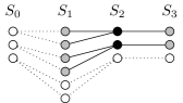
(a)

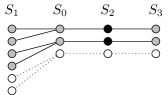
(b)

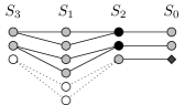
(c)

(d)

Figure 2: Visualization of the properties of a lane $L_{t,t+r}(X)$. Each vertex in the set $X$ is colored black, and the set of reachable vertices in each time step is colored gray. Each figure represents one additional time step. In the second time step (Figure b) all vertices of the lane are reachable. In the third time step (Figure c) one vertex outside the lane must be reachable, for example the diamond shaped vertex. This is due to the fact that the temporal graph at hand is connected, and thus at least one additional vertex is reachable with every next time step. Here, one additional time step then suffices to reach a vertex of $S_{2}\setminus X$ (Figure d).

To describe reachability between orbits, we have to introduce some extra notation. Let $\mathcal{G}$ be a temporal graph with lifetime $\ell$ and vertex set $V$ and $S\in\mathcal{G}/\text{Aut}(\mathcal{G})$ be an orbit. We call a lane $L_{t,t^{\prime}}(X)$ with $X\subseteq S$ and $t,t^{\prime}\in[\ell]$ the set of all vertices reachable from any $u\in X$ in $G$ by any temporal walk $W$ that only uses orbit boundary edges and starts in time step $t$ and ends in time step at most $t^{\prime}$. We write $L_{t,t^{\prime}}(u)$ instead of $L_{t,t^{\prime}}(\{u\})$. See Fig. 2 for some intuition.

The next lemma gives us a lower bound on the number of vertices of an orbit $S^{\prime}$ that can be reached from a subset $X$ of the vertices of an orbit $S$ within $r$ time steps. Intuitively speaking, we show a lower bound on the number of vertices reachable from orbit $S$ in another orbit $S^{\prime}$. A simple consequence of the following lemma is that, from any start vertex in the temporal graph, at least one vertex in every orbit is reachable within $r$ time steps.

Lemma 4.3 (Reachability between Orbits).

Let $\mathcal{G}$ be a connected temporal graph with lifetime $\ell$ and $S\in\mathcal{G}/\text{Aut}(\mathcal{G})$. For any $X\subseteq S$ and $S^{\prime}\in\mathcal{G}/\text{Aut}(\mathcal{G})$ it holds that $|L_{t,t^{\prime}}(X)\cap S^{\prime}|\geq\lceil|X|\cdot|S^{\prime}|/|S|\rceil$ for any $t\in[\ell]$ and $t^{\prime}=t+r$, where $r=|\mathcal{G}/\text{Aut}(\mathcal{G})|$ is the orbit number.

Proof 4.4.

We say an orbit $S^{*}$ is processed for $r^{\prime}$ if $|L_{t,t+r^{\prime}}(X)\cap S^{*}|\geq\lceil|X|\cdot|S^{*}|/|S|\rceil$ for some $r^{\prime}\leq r$, and unprocessed for $r^{\prime}$ otherwise. We now show that as long as unprocessed orbits remain, there exists an orbit $S^{\prime}$ such that $S^{\prime}$ is unprocessed for $r^{\prime}$, but processed for $r^{\prime}+1$, i.e., in each time step at least one unprocessed orbit becomes processed. The lemma then follows simply by counting the number of orbits.

For $r^{\prime}=0$, orbit $S$ is trivially processed for $r^{\prime}$. For $r^{\prime}=1$ note that there exists an orbit $S^{\prime}$ that is adjacent to $S$ in time step $t$. Lemma 4.1 shows that in $G^{\prime}=G^{\prime}_{t}[S\cup S^{\prime}]$ all vertices of $S$ have the same degree $d_{S}$, and all vertices of $S^{\prime}$ have the same degree $d_{S^{\prime}}$, where $G^{\prime}_{t}$ is the subgraph of $G_{t}$ containing only the orbit boundary edges that are present in time step $t$. This implies $|E(G^{\prime})|=|S|\cdot d_{S}=|S^{\prime}|\cdot d_{S^{\prime}}$ and hence $d_{S}/d_{S^{\prime}}=|S^{\prime}|/|S|$. Denote by $E_{X}$ the set of edges incident to vertices of $X$ in $G^{\prime}$. It holds that $|E_{X}|=|X|\cdot d_{S}$. By definition, a vertex $u^{\prime}\in S^{\prime}$ is incident to at most $d_{S^{\prime}}$ edges of $E_{X}$. Denote with $X^{\prime}\subseteq S^{\prime}$ the set of vertices of $S^{\prime}$ that are neighbors of vertices of $X$ in $G^{\prime}$. It holds that $|X^{\prime}|\geq\lceil|X|\cdot d_{S}/d_{S^{\prime}}\rceil=\lceil|X|\cdot|S^{\prime}|/|S|\rceil$. As $L_{t,t+1}(X)\cap S^{\prime}\supseteq X^{\prime}$, this means that $S^{\prime}$ is processed for $r^{\prime}=1$. See Fig. 2(a) for a visualization of this.

For $r^{\prime}$ with $1\leq r^{\prime}<r$, if there is still an unprocessed orbit for $r^{\prime}$, there must exist an unprocessed orbit $S_{u}$ adjacent to a processed orbit $S_{p}$ in time step $t+r^{\prime}$. This follows from the fact that $\mathcal{G}$ is connected. As $S_{p}$ is processed for $r^{\prime}$, we know that the set $X_{p}=L_{t,t^{\prime}}(X)\cap S_{p}$ satisfies $|X_{p}|\geq\lceil|X|\cdot|S_{p}|/|S|\rceil$. By the same argument as in the previous paragraph, it follows that the set $X_{u}\subseteq S_{u}$ of vertices in $S_{u}$ that are neighbors of vertices in $S_{p}$ in time step $t+r^{\prime}$ satisfies $|X_{u}|\geq\lceil|X_{p}|\cdot|S_{u}|/|S_{p}|\rceil\geq\big{\lceil}\lceil|X|\cdot|S_{p}|/|S|\rceil\cdot|S_{u}|/|S_{p}|\big{\rceil}\geq\lceil|X|\cdot|S_{u}|/|S|\rceil$. As $L_{t,t+r^{\prime}+1}(X)\cap S_{u}\supseteq X_{u}$, it follows that $S_{u}$ is processed for $r^{\prime}+1$. As at least one orbit becomes processed in each time step, all orbits are processed latest for $r^{\prime}=r$.

By using Lemma 2.1 and Lemma 4.3, we now bound the number of time steps needed to reach a set of $h$ vertices within an orbit $S$.

Lemma 4.5.

Let $\mathcal{G}$ be a connected temporal graph with lifetime $\ell$ and vertex set $V$. Let $S\in\mathcal{G}/\text{Aut}(\mathcal{G})$ and let $r=|\mathcal{G}/\text{Aut}(\mathcal{G})|$ be the orbit number. For any $h\leq|S|$ and start vertex $u\in S$ and start time $t$, there exists a set $X\subset S$ with $|X|=h$ such that we can reach any vertex in $X$ in at most $O(\min\{h\cdot n/|S|,hr\}+r)$ time steps, i.e., for every vertex $u^{\prime}$ of $X$, we have a temporal walk starting at $u$ at time step $t$ and ending at $u^{\prime}$ at time step $t^{\prime}$ with $t^{\prime}-t=O(\min\{h\cdot n/|S|,hr\}+r)$.

Proof 4.6.

We first show how to reach $h$ vertices in $O(h\cdot n/|S|+r)$ time steps. Denote with $R_{t,t^{\prime}}(u)$ the set of vertices reachable with a temporal walk from $u$ at time step $t$ and ending at or before time step $t^{\prime}$. Our upper bound on the number of time steps required is based on first expanding the set of reachable vertices until we achieve an overflow in some orbit $S^{\prime}\in\mathcal{G}/\text{Aut}(\mathcal{G})$, which we define as $|S^{\prime}\cap R_{t,t^{\prime}}(u)|\geq\texttt{min}\{|S^{\prime}|,\lceil h\cdot|S^{\prime}|/|S|\rceil+1\}$. As $\mathcal{G}$ is connected, we know that, as long as $R_{t,t^{\prime}}(u)\neq V$, $R_{t,t^{\prime}}(u)\subsetneq R_{t,t^{\prime}+1}(u)$ (Lemma 2.1). From this it follows that an overflow exists after at most $\sum_{S^{\prime}\in\mathcal{G}/\text{Aut}(\mathcal{G})}(\lceil h\cdot|S^{\prime}|/|S|\rceil+1)\leq\lceil hn/|S|\rceil+{2}r$ time steps, due to the pigeonhole principle. See Figure 2(c) for an example of an overflow. Let $t^{\prime}$ be the time step when the first overflow occurred, and let $S^{\prime}$ be an orbit where an overflow occurred in time step $t^{\prime}$. Denote by $X^{\prime}$ the set of vertices reachable in $S^{\prime}$ by time step $t^{\prime}$. Using Lemma 4.3 with lane $L_{t^{\prime},t^{\prime}+r}(X^{\prime})$ we know that once an overflow occurs in $S^{\prime}$, after $r$ additional time steps an overflow occurs in all orbits, which guarantees that $h$ vertices in $S$ are reachable: If $R_{t,t^{\prime}}(u)\cap S^{\prime}=S^{\prime}$, Lemma 4.3 implies $|L_{t^{\prime},t^{\prime}+r}\cap S|\geq\lceil|S^{\prime}|\cdot|S|/|S^{\prime}|\rceil=|S|$, meaning all vertices of $S$ are reachable by time $t^{\prime}+r$. If $|R_{t,t^{\prime}}(u)\cap S^{\prime}|\geq\lceil h\cdot|S^{\prime}|/|S|\rceil+1$, Lemma 4.3 implies $|L_{t^{\prime},t^{\prime}+r}\cap S|\geq\lceil(\lceil h\cdot|S^{\prime}|/|S|\rceil+1)\cdot|S|/|S^{\prime}|\rceil\geq h$, meaning that at least $h$ vertices of $S$ are reachable by time $t^{\prime}+r$. In total, $O(h\cdot n/|S|+r)$ time steps always suffice to guarantee an overflow in orbit $S$, which means we can reach $h$ vertices of $S$.

Next, we show how to reach $h$ vertices of $S$ in $O(hr)$ time steps. Let $X$ be the set of reachable vertices of $S$. Initially (in time step $t$) $X=\{u\}$. After $r-1$ time steps all vertices in lane $L_{t,t+r}(X)$ are reachable. By Lemma 4.3, $|L_{t,t+r}(X)\cap S^{\prime}|\geq\lceil|X|\cdot|S^{\prime}|/|S|\rceil$ for any $S^{\prime}\in\mathcal{G}/\text{Aut}(\mathcal{G})$. After one additional time step (Lemma 2.1) there exists some orbit $S^{\prime}$ such that at least one more vertex $v\in S^{\prime}\setminus L_{t,t+r}(X)$ is reachable. See Figure 2(c) for an example of this. So the set $X^{\prime}:=(L_{t,t+r}(X)\cap S^{\prime})\cup\{v\}$ is reachable after $r$ time steps. Note that $|X^{\prime}|\geq\lceil|X|\cdot|S^{\prime}|/|S|\rceil+1$. Using Lemma 4.3 again, now for start time $t+r+1$ and initially reachable vertex set $X^{\prime}$ in orbit $S^{\prime}$, we get that the set $X^{\prime\prime}:=L_{t+r+1,t+2r+1}(X^{\prime})\cap S$ satisfies $|X^{\prime\prime}|\geq\lceil|X^{\prime}|\cdot|S|/|S^{\prime}|\rceil\geq\lceil(\lceil|X|\cdot|S^{\prime}|/|S|\rceil+1)\cdot|S|/|S^{\prime}|\rceil\geq\lceil|X|+|S|/|S^{\prime}|\rceil\geq|X|+1$. Therefore, we can reach a vertex $w$ in $S\setminus X$ by time $t+2r+1$. Repeating the construction with $X=\{u,w\}$ and then with sets $X$ of size $3,\ldots,h-1$, after $O(rh)$ time steps there are $h$ vertices of $S$ reachable.

Next we present Theorem 4.7, which states an upper bound for visiting all vertices of a given orbit $S$. The rough idea used in the proof is that we iteratively build the final temporal walk $W$ by concatenating smaller temporal walks. In each step of the iteration, a small temporal walk is first constructed via Lemma 4.5 to visit a subset of the vertices of $S$, which are not necessarily unvisited, but such that the size of the subset is at least a certain threshold value. We then transform such a small temporal walk into a temporal walk that visits many unvisited vertices of $S$ using Lemma 3.3, and extend $W$ via this transformed walk. In this way we can explore all vertices of a large orbit $S$ faster than by repeated application of Lemma 2.1. The key to obtain a good bound on the number of time steps required is to find a good value for the number of vertices of $S$ visited by each small temporal walk.

Theorem 4.7.

Let $\mathcal{G}$ be a temporal graph with lifetime $\ell$ and vertex set $V$. Take $S\in\mathcal{G}/\text{Aut}(\mathcal{G})$ and $r=|\mathcal{G}/\text{Aut}(\mathcal{G})|$ the orbit number. For any $t\in[\ell]$ there exists a temporal walk $W$ starting at time step $t$ that visits all vertices of $S$ and ends at time step $t^{\prime}$ with $t^{\prime}-t=O((n^{5/3}+rn)\log n)$.

Proof 4.8.

In the following we assume that $|S|=\Omega(n^{2/3})$ as otherwise we can visit all vertices of $S$ in $O(n^{5/3})$ time steps via Lemma 2.1.

We build $W$ iteratively. Initially, $W$ is an empty temporal walk. Denote by $T\subseteq S$ the set of vertices visited by $W$ and by $t_{W}$ the current last time step in which $W$ visits a vertex. First we describe a subroutine that yields a temporal walk $W^{\prime}$ that visits $\lceil n^{1/3}\rceil$ vertices of $S$, but without guarantee that the visited vertices are from $S\setminus T$.

Choose $u\in S$ arbitrarily and let $W^{\prime}$ start at $u$ in time step $t_{W}+n$. Denote with $X$ the set of vertices of $S$ that we have visited so far (initially $X=\{u\}$) during the construction of $W^{\prime}$. Use Lemma 4.5 to extend $W^{\prime}$ by a vertex $u^{\prime}\in S\setminus X$, set $X:=X\cup\{u^{\prime}\}$, and repeat iteratively until $|X|=\lceil n^{1/3}\rceil$. Each application of Lemma 4.5 yields a temporal walk that visits a vertex of $S\setminus X$ in $O((|X|+1)n/|S|+r)$ time steps. Applying Lemma 4.5 $\lceil n^{1/3}\rceil$-times in this fashion yields a temporal walk $W^{\prime}$ that visits $\lceil n^{1/3}\rceil$ vertices of $S$ within $\sum_{i=0}^{\lceil n^{1/3}\rceil}O(i\cdot n/|S|+r)=O(n^{2/3}\cdot n/|S|+rn^{1/3})$ time steps, and as $|S|=\Omega(n^{2/3})$ this is bounded by $O(n+rn^{1/3})$.

By Lemma 3.3 there exists a temporal walk $W_{\sigma}$ that starts at time step $t_{W}+n$ and visits at least $pn^{1/3}$ vertices of $S\setminus T$ with some $v\in S$ the first vertex of $W_{\sigma}$ and $p=(|S|-|T|)/|S|$, which can be obtained by first constructing $W^{\prime}$ as outlined in the previous paragraph and then applying some automorphism $\sigma\in\text{Aut}(\mathcal{G})$ to $W^{\prime}$. By Lemma 2.1 we also know that there exists a temporal walk $W_{v}$ that starts at the vertex where $W$ ends at time step $t_{W}$ and after $n$ time steps ends with the first vertex $v$ of $W_{\sigma}$. We extend $W$ by $W_{v}$ and $W_{\sigma}$. See Figure 3 for a sketch of this idea.

We call one such extension of $W$ a phase and the number of vertices we add to $T$ due to a phase the progress. It is easy to see that as long as $p\geq\frac{1}{2}$ each phase yields at least $\frac{1}{2}n^{1/3}$ progress. It follows that after $n^{2/3}$ phases the fraction $p$ is less than $\frac{1}{2}$. Now, as long as $p\geq\frac{1}{4}$ each phase yields at least $\frac{1}{4}n^{1/3}$ progress, and after $n^{2/3}$ additional phases $p<\frac{1}{4}$. One can see that after $O(n^{2/3}\log n)$ phases we have visited all vertices of $S$. Each phase yields an extension of $W$ that spans $O(n+rn^{1/3})$ time steps, i.e., we have fully constructed $W$ after $O((n^{5/3}+rn)\log n)$ time steps.

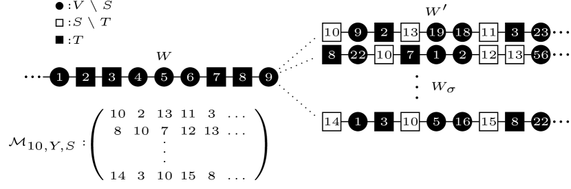
Figure 3: The construction scheme of Theorem 4.7. $W$ is the temporal walk constructed so far. We aim to extend the walk with a walk $W_{\sigma}$ that visits many vertices of $S\setminus T$, where $T$ is the set of vertices of orbit $S$ that we have already visited. To find $W_{\sigma}$, we construct $W^{\prime}$ and the automorphism matrix (bottom left) for the vertex with label $10$ (the start vertex of $W^{\prime}$), the set $Y$ of vertices of $S$ visited by $W^{\prime}$, and the entire orbit $S$ as the set of possible start vertices of $W_{\sigma}$. One of the rows in the matrix then gives us an automorphism $\sigma$ that, when applied to $W^{\prime}$, yields the desired walk $W_{\sigma}$.

The following lemma is concerned with visiting a fraction $1/c$ of the vertices of a given orbit $S$ with a temporal walk. One significant contribution to the number of time steps required by the temporal walk constructed in Theorem 4.7 is the use of Lemma 3.3. Roughly speaking, Lemma 3.3 provides a temporal walk that visits a large number of unvisited vertices, but with the caveat that every vertex of $S$ can potentially be the start vertex of this transformed walk (instead of restricting the potential start vertices for the walk to a smaller subset, which might be reachable more quickly). The consequence of this is that for each such transformation we require, we must plan a “buffer” of $n$ time steps to ensure that all vertices of $S$ are reachable by the time step in which the transformed walk starts (Lemma 2.1). Corollary 3.5 provides a “trade-off” for this: a decrease in the set of possible start vertices of the transformed walk $W_{\sigma}$ decreases the number of previously unvisited vertices $W_{\sigma}$ visits, but also decreases the number of time steps required to reach the first vertex of $W_{\sigma}$. Using this property we construct a recursive algorithm that visits a fraction of the vertices of $S$ quickly instead of applying the iterative construction of Theorem 4.7. In our recursive construction, the walks we concatenate shrink with each recursive call. If we were to use Lemma 3.3 during this, we would have an additional $n$ time steps with each recursive call. Instead, Corollary 3.5 lets us reduce the number of possible start vertices dramatically. The time span required by this walk is then not dependent on $n$, but dependent on $|S|$ and $r$ (the orbit number), and thus is especially useful for exploring smaller orbits. Later in this section we show how this can then be used iteratively to construct a temporal walk that visits all vertices of $S$, which we in turn use to visit all vertices $V$ by visiting all orbits one after the other.

Lemma 4.9.

Let $\mathcal{G}$ be a connected temporal graph with lifetime $\ell$ and vertex set $V$. Let $S\in\mathcal{G}/\text{Aut}(\mathcal{G})$ and let $r=|\mathcal{G}/\text{Aut}(\mathcal{G})|$ be the orbit number. For any $t\in[\ell]$ and any $u\in S$ there exists a temporal walk $W$ that starts at vertex $u$ in time step $t$ and visits a fraction $1/c$ (for any $1<c<\ |S|$) of the vertices of $S$ such that $W$ spans $O(rc(|S|/c)^{\phi(c)}\log|S|)$ time steps, with $\phi(c)=1/(\log{f(c)})$ and $f(c)=(1+(c-1)/c)$.

Proof 4.10.

We use a recursive construction based on the following idea: If we can recursively construct temporal walks that visit $k$ vertices of $S$, then we can construct two such walks $W_{1}$ and $W_{2}$, transform $W_{2}$ into a walk $W_{\sigma}$ that visits $k(c-1)/c$ vertices of $S$ that have not been visited by $W_{1}$, and combine the two walks to get a walk that visits $f(c)\cdot k$ vertices of $S$. By allowing only $ck$ potential start vertices for $W_{\sigma}$, $O(rck)$ time steps suffice for reaching the start vertex of $W_{\sigma}$ from the end vertex of $W_{1}$.

In more detail, assume that, for some $k$ with $1\leq k\leq|S|/c$, $W_{1}$ is a temporal walk starting at a vertex of $S$ at some time step $t^{\prime}$, ending at some time step $t^{\prime\prime}$, and visiting $k$ different vertices of $S$. Denote the set of these $k$ different vertices with $T\subseteq S$. Let $W_{2}$ be an arbitrary temporal walk starting at time step $t^{\prime\prime}+O(rck)$ that also visits $k$ different vertices of $S$, and assume that $W_{2}$ starts at a vertex of $S$. By Corollary 3.5, we know that for any subset $X$ of $S$ of size $ck$ there exists a temporal walk $W_{\sigma}$, obtained by applying an automorphism $\sigma$ to $W_{2}$, that starts at some $x\in X$ and visits $((c-1)/c)k$ vertices of $S\setminus T$.

For any integer $x$, we denote with $T(x)$ the number of time steps our construction scheme requires for a temporal walk that visits $x$ different vertices of $S$, assuming that we start on a vertex of $S$. Then, $T(k)$ time steps suffice to find the initial temporal walk $W_{1}$ as well as $W_{2}$. Lemma 4.5, applied with $h=ck$, lets us reach $ck$ vertices of $S$ within $O(ckr)$ time steps (note that $ck\leq|S|$ since we assume $k\leq|S|/c$). Using those $ck$ vertices as possible start vertices in the application of Corollary 3.5, we can therefore reach the start vertex of $W_{\sigma}$ in $O(ckr)$ time steps.

To construct $W$, we first recursively construct a temporal walk $W_{1}$ starting from $u$ and visiting $k$ vertices of $S$ in $T(k)$ time steps. Afterwards we use $O(rck)$ time steps to construct a set $S^{\mathrm{R}}$ of $ck$ vertices of $S$ that are reachable from the last vertex of $W_{1}$. Taking an arbitrary vertex of $S^{\mathrm{R}}$ as start vertex, we construct a walk $W_{2}$ visiting $k$ vertices of $S$ in $T(k)$ time steps. By using Corollary 3.5, we can turn $W_{2}$ into a walk $W_{\sigma}$ visiting $(c-1)/c\cdot k$ vertices of $S$ that are not yet visited by $W_{1}$. Combining $W_{1}$ with a walk from the last vertex of $W_{1}$ to the start vertex of $W_{\sigma}$ and finally with $W_{\sigma}$ we get a walk $W$ that visits $k+(c-1)/c\cdot k=f(c)k$ vertices of $S$ in $2T(k)+O(rck)$ time steps. Overall, we obtain the recurrence $T(f(c)k)=2T(k)+O(rck)$, which represents the number of time steps used to construct a walk $W$ visiting $f(c)k$ different vertices of $S$ if we start at a vertex of $S$. If we start to expand the recursive calls of the function as shown below (where $\beta$ is the constant hidden in the $O(rck)$ term), we can rewrite the function as a sum:

$$T(k) =\beta rck/f(c)+2T(k/f(c))$$

$$=\beta rck/f(c)+2\beta rck/f^{2}(c)+4T(k/f^{2}(c))$$

$$=\beta rck/f(c)+2\beta rck/f^{2}(c)+4\beta rck/f^{3}(c)+8T(k/f^{3}(c))$$

$$=\ldots$$

Recall that $\phi(c)=1/(\log{f(c)})$. After $\phi(c)\log k=\log_{f(c)}k$ recursive calls (i.e., at recursion depth $\phi(c)\log k$), it is guaranteed that the argument to $T(\cdot)$ is of size at most 1. Due to the number of recursive calls we have at most $2^{\phi(c)\log k}=k^{\phi(c)}$ leaf nodes in the recursion tree, with each such node contributing $T(1)=1$ to the total number of required time steps. We then get:

$$T(k) =\beta rck\sum_{i=1}^{\phi(c)\log k}\frac{1}{2}(\frac{2}{f(c)})^{i}+k^{\phi(c)}$$

$$\leq\frac{\beta rck}{2}(\frac{2}{f(c)})^{\phi(c)\log k}\phi(c)\log k+k^{\phi(c)}$$

$$\leq\frac{\beta rck}{2}(\frac{2}{f(c)})^{\phi(c)(\log_{\frac{2}{f(c)}}k)/(\log_{\frac{2}{f(c)}}2)}\phi(c)\log k+k^{\phi(c)}$$

$$=O(rck^{1+\phi(c)/(\log_{\frac{2}{f(c)}}2)}\log k+k^{\phi(c)})=O(rck^{1+\phi(c)\cdot(\log\frac{2}{f(c)})}\log k+k^{\phi(c)})$$

$$=O(rck^{1+\phi(c)\cdot(1-\log{f(c)})}\log k+k^{\phi(c)})=O(rck^{1+\phi(c)\cdot(1-\frac{1}{\phi(c)})}\log k+k^{\phi(c)})$$

$$=O(rck^{1+\phi(c)-1}\log k+k^{\phi(c)})=O(rck^{\phi(c)}\log k)$$

Thus, we can visit a $1/c$ fraction of the vertices of $S$ in $T(|S|/c)=O(rc(|S|/c)^{\phi(c)}\log|S|)$ time steps.

Corollary 4.11.

Let $\mathcal{G}$ be a temporal graph with lifetime $\ell$ and vertex set $V$. Let $S\in\mathcal{G}/\text{Aut}(\mathcal{G})$ and $r=|\mathcal{G}/\text{Aut}(\mathcal{G})|$ be the orbit number. For any $t\in[\ell]$, any $u\in S$, and any fixed $\epsilon>0$, there exists a temporal walk $W$ that starts at vertex $u$ in time step $t$ and visits some constant fraction $\alpha<1$ of the vertices of $S$ such that $W$ spans $O(r|S|^{1+\epsilon})$ time steps.

Proof 4.12.

Take $f(c)=((c-1)/c)+1)$ and $\phi(c)=1/(\log{f(c)})$ from Lemma 4.9. Note that $\phi(c)$ converges to $1$ from above for $c$ going to infinity. Therefore, for any given constant $\epsilon>0$, there exists a constant $c$ such that $\phi(c)\leq 1+0.9\epsilon$. Applying Lemma 4.9 with that value of $c$ yields a temporal walk with $O(rc(|S|/c)^{\phi(c)}\log|S|)=O(r|S|^{1+0.9\epsilon}\log|S|)=O(r|S|^{1+\epsilon})$ time steps that visits a $\frac{1}{c}$ fraction of the vertices in $S$. We can thus choose $\alpha=\frac{1}{c}$, and the proof is complete.

We now present an improved version of Theorem 4.7 for exploring a whole orbit.

Theorem 4.13.

Let $\mathcal{G}$ be a temporal graph with lifetime $\ell$ and vertex set $V$. Let $S\in\mathcal{G}/\text{Aut}(\mathcal{G})$ and $r=|\mathcal{G}/\text{Aut}(\mathcal{G})|$ be the orbit number. For any $t\in[\ell]$, any $u\in V$, and any fixed $\epsilon>0$, there exists a temporal walk $W$ that starts at vertex $u$ in time step $t$ and visits all vertices of $S$ such that $W$ spans $O(r|S|^{1+\epsilon}+n\log|S|)$ time steps.

Proof 4.14.

The proof is similar to the construction used in Lemma 4.9. We build the final temporal walk iteratively. Initially, $W$ is an empty temporal walk starting at $u$ at time step $t$. Denote by $T$ the set of vertices visited by $W$ and by $t_{W}$ the current last time step of $W$.

Corollary 4.11, applied with $\epsilon^{\prime}=0.9\epsilon$ as the value for $\epsilon$ in the statement of that corollary, can be used to construct a temporal walk $W_{1}$ of $O(r|S|^{1+0.9\epsilon})$ time steps that visits $\alpha|S|$ vertices of $S$, for some constant $\alpha>0$, and starts at time step $t_{W}+n$. Using Lemma 3.3 we can transform $W_{1}$ into a walk $W_{\sigma}$ that visits $p\cdot\alpha|S|$ vertices of $S\setminus T$, with $p=(|S|-|T|)/|S|$. To reach the first vertex of $W_{\sigma}$ in time step $t_{W}+n$ we use standard reachability (Lemma 2.1).

We call one such extension of $W$ a phase and the number of vertices we add to $T$ due to a phase the progress. As long as $p\geq 1/2$ each phase yields at least $\frac{1}{2}\alpha|S|$ progress. It follows that after $1/\alpha$ phases we have visited $|S|/2$ vertices of $S$. Now, as long as $p\geq 1/4$ we make $\frac{1}{4}\alpha|S|$ progress per phase. After $1/\alpha$ such phases we have visited $3|S|/4$ vertices of $S$ in total. We can repeat this scheme for $O(\log|S|)$ phases to visit all vertices of $S$. Between any two consecutive phases we require $n$ time steps to reach the start vertex of the walk $W_{\sigma}$, as outlined in the previous paragraph. In total we get a temporal walk $W$ that spans $O((r|S|^{1+0.9\epsilon}+n)\log|S|)=O(r|S|^{1+\epsilon}+n\log|S|)$ time steps.

By using the theorem above repeatedly for each orbit, we get a temporal walk for the whole temporal graph.

Corollary 4.15.

Let $\mathcal{G}$ be a temporal graph with lifetime $\ell$ and vertex set $V$. For any fixed $\epsilon>0$, there exists a temporal walk $W$ that spans $O(rn^{1+\epsilon})$ time steps and visits all vertices of $V$, where $r=|\mathcal{G}/\text{Aut}(\mathcal{G})|$ is the orbit number.

Proof 4.16.

Visit the orbits one after the other and spend $n$ time steps to go from one orbit to the next (via Lemma 2.1). Let the sizes of the orbits be $n_{1},n_{2},\ldots,n_{r}$. By applying Theorem 4.13, all vertices of an orbit of size $n_{i}$ can be visited in $O(rn_{i}^{1+\epsilon}+n\log n_{i})=O(rn_{i}^{1+\epsilon}+n\log n)$ time steps. All $r$ orbits can therefore be explored in $O(\sum_{i=1}^{r}(rn_{i}^{1+\epsilon}+n\log n))=O(rn^{1+\epsilon}+rn\log n)=O(rn^{1+\epsilon})$ time steps, where the first transformation follows from $\sum n_{i}^{p}\leq(\sum n_{i})^{p}$ for any $p\geq 1$.

5 Upper Bound for TRP

Using Theorem 4.13 we show that trp can be solved by constructing a walk that spans (asymptotically) the same number of steps as a walk for exploring an arbitrary single orbit. The idea is that the two agents identify an orbit in which they meet, and then the first agent moves to this orbit, and after $n$ time steps the second agent starts exploring this orbit. For this the agents must be able to independently identify the same orbit, for which we introduce some additional notation. We extend the definition of isomorphism to temporal graphs as follows. Let $\mathcal{G},\mathcal{H}$ be two temporal graphs with lifetime $\ell$ and vertex sets $V_{\mathcal{G}}$ and $V_{\mathcal{H}}$, respectively. We call a bijection $\theta:V_{\mathcal{G}}\rightarrow V_{\mathcal{H}}$ a temporal isomorphism if $\theta$ is an isomorphism from $G_{t}$ to $H_{t}$ for each $t\in[\ell]$ (and thus also an isomorphism from $G$ to $H$, which denote the underlying graphs of $\mathcal{G}$ and $\mathcal{H}$, respectively). If clear from the context, we say isomorphism instead of temporal isomorphism.

We define an integer coloring as a coloring of the vertices in the vertex set $V$ of a temporal graph $\mathcal{G}$ (with the colors being integer values). The assigned colors induce a partial order $\prec_{\mathcal{P}}$ on the vertex set $V$ such that, for all vertices $u,v\in V$ that are assigned colors $c_{u}$ and $c_{v}$, respectively, with $c_{u}\neq c_{v}$ it holds that $u\prec_{\mathcal{P}}v$ if $c_{u}<c_{v}$. The idea is now that the two agents compute the same integer coloring of the given temporal graph $\mathcal{G}$ with the property that two vertices $u,v\in V$ are assigned the same color $c$ if and only if $u,v\in S$, with $S$ some orbit of $\mathcal{G}/\text{Aut}(\mathcal{G})$. The agents then meet at the smallest orbit, breaking ties via the coloring.

Note that, since the agents do not have access to consistent labels of the vertices in $V$, they are unable to distinguish between two vertices $u,v\in S$ with $S$ being an orbit. Intuitively, the two agents $a_{1}$ and $a_{2}$ view $\mathcal{G}$ as different temporal graphs $\mathcal{G}_{1}$ and $\mathcal{G}_{2}$, respectively, such that $\mathcal{G}_{1}\cong\mathcal{G}\cong\mathcal{G}_{2}$. A natural idea is for the agents to pick a smallest orbit for their meeting, but the challenge is how to ensure that the agents pick the same orbit if there are multiple equal-size orbits that all have the smallest size. Therefore, in the proof of the following lemma we let the agents iterate over all possible temporal graphs until they find a graph $\mathcal{H}$ with $\mathcal{G}_{1}\cong\mathcal{H}\cong\mathcal{G}_{2}$. Then both agents compute an integer coloring for $\mathcal{H}$ as outlined in the previous paragraph. This coloring is translated to a coloring of $\mathcal{G}_{1}$ by agent $a_{1}$ and to a coloring of $\mathcal{G}_{2}$ by agent $a_{2}$ via isomorphism functions, which are independently computed by the agents.

Lemma 5.1.

Let $\mathcal{G}$ be a temporal graph with vertex set $V$ and lifetime $\ell$ and let $a_{1},a_{2}$ be two label-oblivious agents. There exists a pair of programs $(p_{1},p_{2})$ assigned to $a_{1}$ and $a_{2}$, respectively, such that each agent computes the same integer coloring of $V$ and such that two vertices $u,v\in V$ have the same color exactly if $u,v$ are in the same orbit of $\mathcal{G}/{\text{Aut}(\mathcal{G})}$.

Proof 5.2.

Let $I$ be a list of all temporal graphs with $n$ vertices and lifetime $\ell$ such that no two entries of $I$ are isomorphic to each other. For every entry $\mathcal{H}_{i}$ of $I$ we denote with $\mathcal{A}_{\mathcal{H}_{i}}$ a sorted (in arbitrary but deterministic fashion) list of all orbits in $\mathcal{H}_{i}/\text{Aut}(\mathcal{H}_{i})$.

Assume that each of the program $p_{1}$ and $p_{2}$ computes these aforementioned structures. Note that both programs compute the exact same structures as the result is independent of the labels of the temporal graph $\mathcal{G}$ as viewed by agents $a_{1},a_{2}$, respectively.

Let $V_{1}$ and $V_{2}$ denote the vertex set of $\mathcal{G}$ with the labels seen by $p_{1}$ and $p_{2}$, respectively. As the agents are label-oblivious, a vertex in $V$ can have different labels in $V_{1}$ and in $V_{2}$. Denote by $\mathcal{G}_{1}$ and $\mathcal{G}_{2}$ the temporal graph $\mathcal{G}$ with these new labeled vertex sets $V_{1}$ and $V_{2}$, respectively. Keep in mind that $\mathcal{G}_{1}\cong\mathcal{G}\cong\mathcal{G}_{2}$.

Now, both programs $p_{1}$ and $p_{2}$ find the first entry $\mathcal{H}$ in $I$ for which $\mathcal{G}_{1}\cong\mathcal{H}$ and $\mathcal{G}_{2}\cong\mathcal{H}$, respectively. Denote with $\theta_{1}:V_{1}\rightarrow V(\mathcal{H})$ and $\theta_{2}:V_{2}\rightarrow V(\mathcal{H})$ arbitrary isomorphisms computed by $p_{1}$ and $p_{2}$, respectively. The intuitive goal is now that both agents compute an integer coloring for $\mathcal{H}$ as sketched previously, and this coloring is translated to a coloring of $\mathcal{G}$ via these isomorphism functions.

We now show how to assign the colors to vertices. For $k=1,2$, the program $p_{k}$ iterates over all $S_{i}\in\mathcal{H}/\text{Aut}(\mathcal{H})$ (which are precomputed and sorted in a deterministic but arbitrary fashion) and for each $S_{i}$ assigns the color $i$ to all vertices in $\{\theta_{k}^{-1}(u)\mid u\in S_{i}\}$. Note that both programs iterate over $\mathcal{H}/\text{Aut}(\mathcal{H})$ in the same order.

It remains to show that the coloring computed by $p_{1}$ is the same as the coloring computed by $p_{2}$. Assume for a contradiction that a vertex $u$ in $\mathcal{G}$ is colored differently by $p_{1}$ and $p_{2}$. Let $u_{1}$ and $u_{2}$ be the names of $u$ in $\mathcal{G}_{1}$ and $\mathcal{G}_{2}$, respectively. Since $u$ is colored differently by $p_{1}$ and $p_{2}$, vertices $v=\theta_{1}(u_{1})$ and $w=\theta_{2}(u_{2})$ are in different orbits of $\mathcal{H}/\text{Aut}(\mathcal{H})$. Moreover, since $u_{1}$ and $u_{2}$ is the same vertex, there is an isomorphism $\sigma$ between $\mathcal{G}_{1}$ and $\mathcal{G}_{2}$ that maps $u_{1}$ to $u_{2}$. Now we get an automorphism $\theta_{2}\circ\sigma\circ\theta_{1}^{-1}$ of $\mathcal{H}$ that maps $v$ to $w$, and thus $v$ and $w$ are in the same orbit of $\mathcal{H}/\text{Aut}(\mathcal{H})$, a contradiction.

We can now easily construct an algorithm for trp. The agents can simply meet in a smallest orbit, breaking ties via the integer coloring (Lemma 5.1). The first agent moves to said orbit, and then the second agent searches the orbit for the first agent. Note that the smallest orbit is of size at most $n/r$, where $r$ is the orbit number. Thus, the bound on the number of time steps provided by Theorem 4.13 becomes $O(r(n/r)^{1+\epsilon}+n\log(n/r))=O(n^{1+\epsilon})$, and we obtain the following upper bound for trp.

Theorem 5.3.

Let $\mathcal{G}$ be a temporal graph with lifetime $\ell$ and $a_{1},a_{2}$ two label-oblivious agents. For any fixed $\epsilon>0$, there exists a pair of programs $(p_{1},p_{2})$ assigned to $a_{1},a_{2}$, respectively, such that the two agents are guaranteed to meet after $O(n^{1+\epsilon})$ time steps.

6 Lower Bounds for TEXP and TRP

We start this section with a simple lower bound for texp, which is a fairly straightforward adaptation of the known lower bound of $\Omega(n^{2})$ time steps [26]. Following that, we give a lower bound of $\Omega(n\log n)$ time steps for trp. For this we describe the construction of a temporal graph that is connected and has only a single orbit. We then show how an adversary can choose the starting positions of the two agents that want to meet in order to delay their meeting. Intuitively, the graph we create is a cycle that changes repeatedly after some number of steps. By our construction, the adversary can make sure that after every change of the graph, the two agents are placed far away from each other. In the end, we also show that the resulting lower bound for trp yields a corresponding lower bound for texp.

Lemma 6.1.

For any $1\leq r\leq n$, there exist $n$-vertex instances of texp with orbit number $r$ that require $\Omega(rn)$ time steps to be explored.

Proof 6.2.

Assume without loss of generality that $n$ is even. For $r=1$, the lower bound is trivial as any $n$-vertex temporal graph requires $\Omega(n)$ time steps to be explored. Next, assume $2\leq r\leq\frac{n}{2}$. The lower bound of $\Omega(n^{2})$ presented by Erlebach et al. [26] is based on the construction of a temporal graph $\mathcal{G}$ with vertex set $V$ and lifetime $\ell$ such that at each time step $t\in[\ell]$ the graph $G_{t}$ forms a star as follows: the vertex set $V$ is partitioned into two sets $A$ and $B$, each of size $\frac{n}{2}$. We modify this construction by letting $A$ consists of $r-1$ vertices and $B$ of the remaining vertices. In each of the first $r-1$ time steps, a different vertex of $A$ is chosen to be the center of the star. Vertices of $B$ are never centers of a star. This pattern repeats, i.e., in each time step $t>r-1$, the graph $G_{t}$ is equal to the graph $G_{t-(r-1)}$. The lifetime of the graph is set to $\ell=n^{2}$. By construction, all vertices of $A$ form their own orbit of size $1$ (each center is uniquely identified by the first time step where it is a center), and all vertices of $B$ form one orbit together. Thus, the graph has $(r-1)+1=r$ orbits. As shown by Erlebach et al., it takes $\Theta(r)$ time steps to go from one vertex of $B$ to another. Thus, visiting all vertices, in particular those in $B$, takes $\Omega(r|B|)=\Omega(rn)$ time steps. Here, we have used that $r\leq\frac{n}{2}$ implies $|B|\geq\frac{n}{2}+1$.

Finally, if $\frac{n}{2}<r\leq n$, use the construction above for $r=\frac{n}{2}$ to create a temporal graph with $n^{2}$ time steps that requires $\Omega(n^{2})$ time steps for exploration. Then, add one extra time step $t_{f}=n^{2}+1$ to split the orbit $B$ into the required number of orbits as follows. Assume we want to have orbit number $\frac{n}{2}+k$ for some $1\leq k\leq\frac{n}{2}$. Then $G_{f}$ consists of a path $P$ of $\frac{n}{2}+k-1$ vertices, made up of the $\frac{n}{2}-1$ vertices from $A$ followed by $k$ vertices from $B$, while the remaining $\frac{n}{2}+1-k$ vertices of $B$ are attached as pendant vertices to the endpoint of the path $P$ that lies in $B$. The vertices of $B$ are split into $k+1$ orbits in this way: each of the vertices on $P$ forms an orbit by itself, while those attached as pendants to an endpoint of $P$ form one orbit together. Thus, the temporal graph has orbit number $\frac{n}{2}+k$, as desired.

Theorem 6.3.

For any two agents $a_{1}$ and $a_{2}$ with arbitrary deterministic programs, there exist instances of trp where the agents require $\Omega(n\log n)$ time steps to meet.

Proof 6.4.

We construct a temporal graph $\mathcal{G}=(G_{1},\dots,G_{\ell})$ with lifetime $\ell=n^{2}$ and vertex set $V=\{0,\dots,n-1\}$ with $n=2^{m}-1$ for an arbitrarily large odd integer $m>10$. We define the static graph $C_{i}$ with vertex set $V$ to be the cycle where each vertex $u\in V$ is adjacent to vertices $(u+n_{i})\bmod n$ (the clockwise neighbor) and $(u-n_{i})\bmod n$ (the counter-clockwise neighbor) for $n_{i}=2^{2i}$. Note that $C_{i}$ is indeed a cycle because $n_{i}=2^{2i}$ and $n=2^{m}-1$ are coprime. In what follows we use $n_{i}$ and $2^{2i}$ interchangeably. For our construction (see Fig. 4 for an illustration), we will use the cycles $C_{i}$ for $i\in\{0\}\cup\{2,3,\ldots,\frac{m-7}{2}\}$, i.e., we will use the cycles $C_{0},C_{2},C_{3},C_{4},\ldots,C_{(m-7)/2}$. For each cycle $C_{i}$, we define the $k$-th section of the cycle as $S_{i,k}=\{u\mid u\in V\text{ and }u\bmod 2^{2i}=k\}$. There are $2^{2i}$ different sections in cycle $i$, one for each $k$ with $0\leq k<2^{2i}$. Each one contains $\lceil\frac{n}{2^{2i}}\rceil$ vertices, except the last one which contains $\lfloor\frac{n}{2^{2i}}\rfloor$ vertices due to parity reasons ($n$ is an odd number that is one smaller than a power of two). Intuitively, a section contains vertices with the same modulo value, and these vertices (in ascending order) form a consecutive part of the cycle $C_{i}$. Note that any $s$ sections contain together at least $s\cdot\frac{n}{2^{2i}}-1$ vertices. The first and last vertex of a section is connected to the last vertex of the previous section and the first one of the next section, respectively.

Furthermore, we define phase $i$, for $i\geq 1$, of $\mathcal{G}$ as a number of consecutive time steps from $t\in[\ell]$ to $t^{\prime}\in[\ell]$ such that $G_{t^{\prime\prime}}=G_{t}$ for all $t\leq t^{\prime\prime}\leq t^{\prime}$ and $G_{t-1}\neq G_{t}$ (or $t=1$) and $G_{t^{\prime}}\neq G_{t^{\prime}+1}$. We set the duration of each phase to $K=\lfloor n/16\rfloor$. During phase $1$, the graphs $G_{t}$ are all equal to $C_{0}$. During phase $i$ for $i>1$, the graphs $G_{t}$ are all equal to $C_{i}$. We continue the construction for $(m-7)/2=\Theta(\log n)$ phases.

Notice that the temporal graph $\mathcal{G}$ is constructed in such a way that it has only one orbit as for every $d$ the function $\sigma$ with $\sigma(u)=(u+d)\bmod n$ for all $u\in V$ is an automorphism. Hence, the vertices are indistinguishable to the two agents. Therefore, the deterministic programs that the agents run must execute a sequence of steps that is independent of the starting vertex. (The adversary can let each agent see vertex labels that make the agent’s view the same no matter in which vertex of $\mathcal{G}$ the agent is placed at time $1$.) The steps executed by an agent can be either edge traversals (clockwise or counter-clockwise) or waiting at a current vertex. In what follows, we show that independently of the sequence of steps that each agent’s program performs, an adversary can choose the starting vertex for each agent in such a way that they will need $\Omega(n\log n)$ time steps to meet.

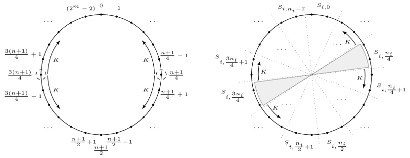
Figure 4: The initial cycle of phase $1$, $C_{0}$, on the left. Initially, the agents are placed on the vertices marked with dashed circles and can move up to $K$ vertices away in phase $1$. In each other phase $i\geq 2$, the cycle $C_{i}$ is viewed as consisting of sections, as shown on the right. At the beginning of the phase, the agents are placed in vertices of two sections (shown grey) that are sufficiently far apart, and they can move up to $K$ vertices away from the boundary of their section before the next phase starts.

We are going to use bit vectors of length $m=\lceil\log n\rceil$ to represent a vertex, i.e., the bit vector $\vec{b}=(b_{m-1}b_{m-2}\dots b_{1}b_{0})$ refers to the vertex whose binary representation is $\vec{b}$. Initially, we place the agent $a_{1}$ at vertex $u=\frac{1}{4}(n+1)$ and agent $a_{2}$ at vertex $v=\frac{3}{4}(n+1)$ of $C_{0}$. Note that the binary representation of $u$ is $(010\cdots 0)$ and that of $v$ is $(110\cdots 0)$, i.e., the lowest $m-2$ bits of both bit vectors are all zero.

During phase $1$, each agent can move up to $K$ vertices away from its start vertex. Given the initial placement of the agents and the size of the cycle, it is guaranteed that they cannot meet in phase $1$: Their initial distance is roughly $n/2$, and even if both of them move $K$ steps closer to the other agent, their distance will only reduce by $2K\leq n/8$. Furthermore, even if we shift each agent’s start vertex by at most $n/8$ positions, they still cannot meet in phase $1$: Their initial distance will be at least roughly $n/4$, and their distance can reduce by at most $n/8$ in phase $1$. We will actually shift the start positions of both agents only by fixing the lowest $m-5$ bits of their bit vectors, so their start positions will be shifted by at most $2^{m-5}-1\leq n/32$, and it is clear that the agents will not be able to meet in phase $1$ no matter what the exact amount of shift is. Our strategy will be to fix the lower-order bits of the start positions of the agents in such a way that the agents cannot meet in phase $i$ for $2\leq i\leq\frac{m-7}{2}$ either.

By adjusting the lowest $4$ bits of $u$ and $v$, i.e., bits $b_{0},b_{1},b_{2},b_{3}$ of their respective bit vectors, we can ensure that agent $a_{1}$ ends phase $1$ at a vertex $u_{1}$ with $u_{1}\bmod{16}=4$ and agent $a_{2}$ ends phase $1$ at a vertex $u_{2}$ with $u_{2}\bmod{16}=12$. This is because fixing the bits $b_{0},b_{1},b_{2},b_{3}$ in one of the 16 possible ways will add an offset $\Delta\in\{0,1,2,\ldots,15\}$ to the start position of an agent, and the same offset is added to the position in which the agent ends phase $1$ (because every edge traversal adds or subtracts a fixed value to the current position). As the agents end phase $1$ in vertices $u_{1}$ and $u_{2}$ satisfying $u_{1}\bmod{16}=4$ and $u_{2}\bmod{16}=12$, the first agent is placed in a vertex in section $S_{2,\frac{1}{4}2^{2\cdot 2}}=S_{2,4}$ of $C_{2}$ while the second agent is placed in a vertex in section $S_{2,\frac{3}{4}2^{2\cdot 2}}=S_{2,12}$ of $C_{2}$ in the beginning of phase $2$. Sections $S_{2,4}$ and $S_{2,12}$ are separated by seven other sections, which together span at least $7\cdot\frac{n}{16}-1\geq n/4$ vertices. Therefore, the agents cannot meet during phase $2$.

Now, depending on the sequence of steps taken by the two agents in phase $2$, we will show that it suffices for the adversary to fix the next two bits, i.e., bit $b_{4}$ and $b_{5}$ of the bit vectors of the start positions of the two agents, in order to guarantee that the two agents are placed sufficiently far from each other at the beginning of phase $3$ and therefore cannot meet in that phase either. Observe that fixing bits $b_{4}$ and $b_{5}$ does not change the value of $u_{1}\bmod 16$ and $u_{2}\bmod 16$. Thus, the sections in which the agents begin phase $2$ are not altered by fixing bits $b_{4}$ and $b_{5}$. This process then repeats for all phases $i>2$: Depending on the sequence of steps taken by the agents in phase $i$, the adversary fixes bits $b_{2i}$ and $b_{2i+1}$ of the binary representations in such a way that the agents begin phase $i+1$ in sections of $C_{i+1}$ that are sufficiently far from each other (without altering the sections in which the agents have started any of the previous phases).

We have already shown that the two agents cannot meet in phase $1$ or $2$. In the following, we show how to fix bits $b_{2i}$ and $b_{2i+1}$ at the end of phase $i$ for $i\geq 2$ in such a way that the two agents cannot meet in phase $i+1$ (in cycle $C_{i+1}$) either.

At the end of phase $i$, we have four options to choose from for the section of $C_{i+1}$ where we would like agent $a_{1}$ to start phase $i+1$. Let $z$ be the value determined by the lowest $2i$ bits of $a_{1}$’s current position (at the end of phase $i$). Note that $z\leq 2^{2i}-1<\frac{1}{4}\cdot 2^{2(i+1)}=\frac{1}{4}n_{i+1}$. The four choices $00$, $01$, $10$ and $11$ for bits $b_{2i}$ and $b_{2i+1}$ of $a_{1}$’s start position produce positions for $a_{1}$ at the end of phase $i$ that are equal to $z$, $z+2^{2i}$, $z+2\cdot 2^{2i}$, and $z+3\cdot 2^{2i}$ modulo $2^{2(i+1)}$, corresponding to sections $S_{i+1,z}$, $S_{i+1,z+\frac{1}{4}n_{i+1}}$, $S_{i+1,z+\frac{1}{2}n_{i+1}}$, $S_{i+1,z+\frac{3}{4}n_{i+1}}$ of $C_{i+1}$. Analogously, there is a $z^{\prime}<\frac{1}{4}n_{i}$ such that agent $a_{2}$ can be placed in any of the four sections $S_{i+1,z^{\prime}}$, $S_{i+1,z^{\prime}+\frac{1}{4}n_{i+1}}$, $S_{i+1,z^{\prime}+\frac{1}{2}n_{i+1}}$, $S_{i+1,z^{\prime}+\frac{3}{4}n_{i+1}}$ of $C_{i+1}$ at the start of phase $i+1$. We choose bits $b_{2i}$ and $b_{2i+1}$ for $a_{1}$ and $a_{2}$ in such a way that $a_{1}$ begins phase $i+1$ in $S_{i+1,z}$ and $a_{2}$ begins phase $i+1$ in $S_{i+1,z^{\prime}+\frac{1}{2}n_{i+1}}$. The sections in which the two agents start phase $i+1$ are then separated by at least $\frac{1}{4}n_{i+1}$ sections in $C_{i+1}$, and these $\frac{1}{4}n_{i+1}$ sections contain together at least $\frac{1}{4}n_{i+1}\cdot\frac{n}{n_{i+1}}-1=\frac{n}{4}-1$ vertices. As each agent can move over at most $K=\lfloor n/16\rfloor$ vertices in phase $i+1$, it is impossible for the agents to meet in phase $i+1$.

We iterate this construction until phase $\frac{m-7}{2}$. (For all time steps from the end of phase $\frac{m-7}{2}$ until the lifetime $\ell=n^{2}$ is reached, we can let the graph be equal to $C_{0}$.) By construction, the agents cannot meet in any of the phases from $i$ to $\frac{m-7}{2}$. As we have fixed the four lowest bits of the start positions of the two agents at the end of phase $1$ and fixed two further bits in each of the remaining $\frac{m-9}{2}$ phases, we have fixed the lowest $4+(m-9)=m-5$ bits of the start positions in this way. As observed at the start of the proof, this ensures that the agents cannot meet in phase $1$ either. Hence, there are $\frac{m-7}{2}=\Theta(\log n)$ phases, each with $\lfloor n/16\rfloor$ time steps, during which the adversary can prevent the agents from meeting. This shows that $\Omega(n\log n)$ time steps are needed for the agents to meet.

Corollary 6.5.

There exist connected temporal graphs $\mathcal{G}$ with vertex set $V$, lifetime $\ell$ and a single orbit such that all temporal walks $W$ require $\Omega(n\log n)$ time steps to visit all vertices of $V$.

Proof 6.6.

Assume for a contradiction that for every connected temporal graph $\mathcal{G}$ with $n$ vertices and a single orbit there exists a temporal walk that visits all vertices in $o(n\log n)$ time steps. This implies that trp can be solved in $o(n\log n)$ time steps for connected single-orbit temporal graphs: Let the agent $a_{1}$ perform a temporal walk that visits all vertices in $o(n\log n)$ time steps, and let the agent $a_{2}$ remain at its initial vertex. By Theorem 6.3, no such solution to trp is possible.

The lower bounds of Theorem 6.3 and Corollary 6.5 can be adapted to temporal graphs with $r$ orbits for any constant $r$ as follows: Use the construction from the proof of Theorem 6.3, but instead of letting the graph $G_{t}$ in each time step be a single cycle $C_{i}$, let $G_{t}$ contain $2r-1$ copies of $C_{i}$, and for each vertex $u$ of $C_{i}$ connect all copies of $u$ by a path $P_{u}$ (starting with the vertex $u$ in the first copy of $C_{i}$ and ending with the vertex $u$ in the $(2r-1)$-th copy of $C_{i}$). The resulting temporal graph has $r$ orbits: The vertices of the ‘middle’ copy of $C_{i}$ form one orbit, and the vertices in the two copies of $C_{i}$ that have distance $k$ from the middle copy, for $1\leq k\leq r-1$, also form an orbit. Let $n^{\prime}=n/r$ denote the number of vertices in one copy of $C_{i}$. By the arguments in the proof of Theorem 6.3, it takes $\Omega(n^{\prime}\log n^{\prime})$ time steps for the two agents to reach a location in the same path $P_{u}$, and thus trp requires $\Omega(n^{\prime}\log n^{\prime})$ time steps. As $n^{\prime}=n/r$ and $r$ is a constant, this gives a lower bound of $\Omega(n\log n)$ for trp. The lower bound of $\Omega(n\log n)$ time steps for exploration of temporal graphs with orbit number $r$ for any constant $r$ then follows as in the proof of Corollary 6.5.

7 Conclusions & Future Work

In this work, we looked at temporal graphs where agents know the complete information of the temporal graph ahead of time. In this clairvoyant setting, we studied the temporal exploration problem (texp) and showed how to bound the exploration time of a temporal graph using the structural graph property of the number of orbits of the automorphism group of the temporal graph. Additionally, we formalized the problem of asymmetric rendezvous in this setting as the temporal rendezvous problem (trp) and showed how to adapt our ideas for texp to solve trp quickly. For both texp and trp we provided lower bounds such that the gap between upper and lower bounds is $O(n^{\epsilon})$ for any fixed $\epsilon>0$.

There are several ways in which our work can be extended. One line of research for both problems is to reduce the gap between the lower and upper bounds by improving either of them. A second line of work is to study the symmetric variant of rendezvous in the given setting and see if something can be said about it. Another interesting situation to explore is when multiple agents are used to explore the temporal graph (and also if multiple agents need to perform temporal rendezvous) and how much faster solutions in these scenarios might be.

Lastly, a possible avenue of research is to study the structural properties provided by automorphism groups and how they can be used to tackle other problems that concern temporal graphs.

References

- [1] Eric Aaron, Danny Krizanc, and Elliot Meyerson. Dmvp: foremost waypoint coverage of time-varying graphs. In International Workshop on Graph-Theoretic Concepts in Computer Science, pages 29–41. Springer, 2014. doi:10.1007/978-3-319-12340-0_3.
- [2] Eric Aaron, Danny Krizanc, and Elliot Meyerson. Multi-robot foremost coverage of time-varying graphs. In International Symposium on Algorithms and Experiments for Sensor Systems, Wireless Networks and Distributed Robotics, pages 22–38. Springer, 2014. doi:10.1007/978-3-662-46018-4_2.
- [3] Duncan Adamson, Vladimir V. Gusev, Dmitriy Malyshev, and Viktor Zamaraev. Faster exploration of some temporal graphs. In 1st Symposium on Algorithmic Foundations of Dynamic Networks (SAND 2022). Schloss Dagstuhl-Leibniz-Zentrum für Informatik, 2022. doi:10.4230/LIPIcs.SAND.2022.5.
- [4] Eleni C. Akrida, Jurek Czyzowicz, Leszek Gąsieniec, Łukasz Kuszner, and Paul G. Spirakis. Temporal flows in temporal networks. Journal of Computer and System Sciences, 103:46–60, 2019. doi:10.1016/j.jcss.2019.02.003.
- [5] Eleni C. Akrida, George B. Mertzios, Paul G. Spirakis, and Christoforos Raptopoulos. The temporal explorer who returns to the base. Journal of Computer and System Sciences, 120:179–193, 2021. doi:10.1016/j.jcss.2021.04.001.
- [6] Eleni C. Akrida, George B. Mertzios, Paul G. Spirakis, and Viktor Zamaraev. Temporal vertex cover with a sliding time window. Journal of Computer and System Sciences, 107:108–123, 2020. doi:10.1016/j.jcss.2019.08.002.
- [7] S. Alpern and S. Gal. The Theory of Search Games and Rendezvous. International Series in Operations Research & Management Science. Springer US, 2006. doi:10.1007/b100809.
- [8] Steve Alpern. The rendezvous search problem. SIAM Journal on Control and Optimization, 33(3):673–683, 1995. doi:10.1137/S0363012993249195.
- [9] Steve Alpern. Rendezvous search: A personal perspective. Operations Research, 50(5):772–795, 2002. doi:10.1287/opre.50.5.772.363.
- [10] Steve Alpern and Shmuel Gal. The theory of search games and rendezvous, volume 55. Springer Science & Business Media, 2006. doi:10.1007/b100809.
- [11] Steven Alpern. Hide and seek games. In Seminar, Institut für höhere Studien, Wien, volume 26, 1976.
- [12] K. Balasubramanian. Symmetry groups of chemical graphs. International Journal of Quantum Chemistry, 21(2):411–418, 1982. doi:10.1002/qua.560210206.
- [13] Fabian Ball and Andreas Geyer-Schulz. How symmetric are real-world graphs? a large-scale study. Symmetry, 10(1), 2018. doi:10.3390/sym10010029.
- [14] Subhash Bhagat and Andrzej Pelc. Deterministic rendezvous in infinite trees. CoRR, abs/2203.05160, 2022. arXiv:2203.05160, doi:10.48550/arXiv.2203.05160.
- [15] Hans L. Bodlaender and Tom C. van der Zanden. On exploring always-connected temporal graphs of small pathwidth. Information Processing Letters, 142:68–71, 2019. doi:10.1016/j.ipl.2018.10.016.
- [16] John Adrian Bondy and Uppaluri Siva Ramachandra Murty. Graph theory with applications, volume 290. Macmillan London, 1976.
- [17] Marjorie Bournat, Swan Dubois, and Franck Petit. Gracefully degrading gathering in dynamic rings. In Stabilization, Safety, and Security of Distributed Systems: 20th International Symposium, SSS 2018, Tokyo, Japan, November 4–7, 2018, Proceedings 20, pages 349–364. Springer, 2018. doi:10.1007/978-3-030-03232-6_23.
- [18] Benjamin Merlin Bumpus and Kitty Meeks. Edge exploration of temporal graphs. Algorithmica, 85(3):688–716, 2023. doi:10.1007/s00453-022-01018-7.
- [19] Arnaud Casteigts, Paola Flocchini, Walter Quattrociocchi, and Nicola Santoro. Time-varying graphs and dynamic networks. Int. J. Parallel Emergent Distributed Syst., 27(5):387–408, 2012. doi:10.1080/17445760.2012.668546.
- [20] Jurek Czyzowicz, Adrian Kosowski, and Andrzej Pelc. How to meet when you forget: Log-space rendezvous in arbitrary graphs. In Proceedings of the 29th ACM SIGACT-SIGOPS Symposium on Principles of Distributed Computing, PODC ’10, page 450–459, New York, NY, USA, 2010. Association for Computing Machinery. doi:10.1145/1835698.1835801.
- [21] Shantanu Das, Giuseppe Di Luna, Linda Pagli, and Giuseppe Prencipe. Compacting and grouping mobile agents on dynamic rings. In International Conference on Theory and Applications of Models of Computation, pages 114–133. Springer, 2019. doi:10.1007/978-3-030-14812-6_8.
- [22] Giuseppe Antonio Di Luna. Mobile agents on dynamic graphs. Distributed Computing by Mobile Entities: Current Research in Moving and Computing, pages 549–584, 2019. doi:10.1007/978-3-030-11072-7_20.
- [23] Giuseppe Antonio Di Luna, Paola Flocchini, Linda Pagli, Giuseppe Prencipe, Nicola Santoro, and Giovanni Viglietta. Gathering in dynamic rings. Theoretical Computer Science, 811:79–98, 2020. doi:10.1016/j.tcs.2018.10.018.
- [24] Yoann Dieudonné, Andrzej Pelc, and Vincent Villain. How to meet asynchronously at polynomial cost. In Proceedings of the 2013 ACM symposium on Principles of distributed computing, pages 92–99, 2013. doi:10.1137/130931990.
- [25] Jessica Enright, Kitty Meeks, George B. Mertzios, and Viktor Zamaraev. Deleting edges to restrict the size of an epidemic in temporal networks. Journal of Computer and System Sciences, 119:60–77, 2021. doi:10.1016/j.jcss.2021.01.007.
- [26] Thomas Erlebach, Michael Hoffmann, and Frank Kammer. On temporal graph exploration. J. Comput. Syst. Sci., 119:1–18, 2021. doi:10.1016/j.jcss.2021.01.005.
- [27] Thomas Erlebach, Frank Kammer, Kelin Luo, Andrej Sajenko, and Jakob T. Spooner. Two moves per time step make a difference. In 46th International Colloquium on Automata, Languages, and Programming (ICALP 2019). Schloss Dagstuhl-Leibniz-Zentrum für Informatik, 2019. doi:10.4230/LIPIcs.ICALP.2019.141.
- [28] Thomas Erlebach and Jakob T. Spooner. Exploration of k-edge-deficient temporal graphs. Acta Informatica, 59(4):387–407, 2022. doi:10.1007/s00236-022-00421-5.
- [29] Thomas Erlebach and Jakob T. Spooner. Parameterized temporal exploration problems. In 1st Symposium on Algorithmic Foundations of Dynamic Networks, SAND 2022, March 28-30, 2022, Virtual Conference, volume 221 of LIPIcs, pages 15:1–15:17. Schloss Dagstuhl - Leibniz-Zentrum für Informatik, 2022. doi:10.4230/LIPIcs.SAND.2022.15.
- [30] Paola Flocchini. Distributed Computing by Mobile Entities: Current Research in Moving and Computing. Springer, 2019. doi:10.1007/978-3-030-11072-7.
- [31] Till Fluschnik, Hendrik Molter, Rolf Niedermeier, Malte Renken, and Philipp Zschoche. As time goes by: Reflections on treewidth for temporal graphs. In Treewidth, Kernels, and Algorithms: Essays Dedicated to Hans L. Bodlaender on the Occasion of His 60th Birthday, pages 49–77. Springer International Publishing, 2020. doi:10.1007/978-3-030-42071-0_6.
- [32] Till Fluschnik, Hendrik Molter, Rolf Niedermeier, Malte Renken, and Philipp Zschoche. Temporal graph classes: A view through temporal separators. Theoretical Computer Science, 806:197–218, 2020. doi:10.1016/j.tcs.2019.03.031.
- [33] Chris Godsil and Gordon F. Royle. Algebraic Graph Theory. Number Book 207 in Graduate Texts in Mathematics. Springer, 2001. doi:10.1007/978-1-4613-0163-9.
- [34] Thekla Hamm, Nina Klobas, George B. Mertzios, and Paul G. Spirakis. The complexity of temporal vertex cover in small-degree graphs. Proceedings of the AAAI Conference on Artificial Intelligence, 36(9):10193–10201, Jun. 2022. doi:10.1609/aaai.v36i9.21259.
- [35] David Ilcinkas, Ralf Klasing, and Ahmed Mouhamadou Wade. Exploration of constantly connected dynamic graphs based on cactuses. In International Colloquium on Structural Information and Communication Complexity, pages 250–262. Springer, 2014. doi:10.1007/978-3-319-09620-9_20.
- [36] David Ilcinkas and Ahmed Mouhamadou Wade. Exploration of the t-interval-connected dynamic graphs: the case of the ring. In International Colloquium on Structural Information and Communication Complexity, pages 13–23. Springer, 2013. doi:10.1007/978-3-319-03578-9_2.
- [37] Ulrich Knauer and Kolja Knauer. Algebraic graph theory: morphisms, monoids and matrices, volume 41. Walter de Gruyter GmbH & Co KG, 2019. doi:10.1515/9783110617368.
- [38] Evangelos Kranakis, Danny Krizanc, and Euripides Marcou. The mobile agent rendezvous problem in the ring. Springer Nature, 2022. doi:10.1007/978-3-031-01999-9.
- [39] Evangelos Kranakis, Danny Krizanc, and Sergio Rajsbaum. Mobile agent rendezvous: A survey. In Structural Information and Communication Complexity, pages 1–9. Springer Berlin Heidelberg, 2006. doi:10.1007/11780823_1.
- [40] Josef Lauri and Raffaele Scapellato. Topics in Graph Automorphisms and Reconstruction. Cambridge University Press, 2016. doi:10.1017/CBO9781316669846.
- [41] Gianluca De Marco, Luisa Gargano, Evangelos Kranakis, Danny Krizanc, Andrzej Pelc, and Ugo Vaccaro. Asynchronous deterministic rendezvous in graphs. Theoretical Computer Science, 355(3):315–326, 2006. doi:10.1016/j.tcs.2005.12.016.
- [42] Andrea Marino and Ana Silva. Königsberg sightseeing: Eulerian walks in temporal graphs. In Combinatorial Algorithms, pages 485–500. Springer International Publishing, 2021. doi:10.1007/978-3-030-79987-8_34.
- [43] Andrea Marino and Ana Silva. Coloring temporal graphs. Journal of Computer and System Sciences, 123:171–185, 2022. doi:10.1016/j.jcss.2021.08.004.
- [44] George B. Mertzios, Hendrik Molter, Rolf Niedermeier, Viktor Zamaraev, and Philipp Zschoche. Computing Maximum Matchings in Temporal Graphs. In 37th International Symposium on Theoretical Aspects of Computer Science (STACS 2020), volume 154 of Leibniz International Proceedings in Informatics (LIPIcs), pages 27:1–27:14, Dagstuhl, Germany, 2020. Schloss Dagstuhl–Leibniz-Zentrum für Informatik. doi:10.4230/LIPIcs.STACS.2020.27.
- [45] George B. Mertzios, Hendrik Molter, and Viktor Zamaraev. Sliding window temporal graph coloring. Journal of Computer and System Sciences, 120:97–115, 2021. doi:10.1016/j.jcss.2021.03.005.
- [46] Othon Michail. An introduction to temporal graphs: An algorithmic perspective. Internet Math., 12(4):239–280, 2016. doi:10.1080/15427951.2016.1177801.
- [47] Othon Michail and Paul G. Spirakis. Traveling salesman problems in temporal graphs. Computer Science (MFCS), 2014. doi:10.1016/j.tcs.2016.04.006.
- [48] Othon Michail and Paul G. Spirakis. Traveling salesman problems in temporal graphs. Theoretical Computer Science, 634:1–23, 2016. doi:10.1016/j.tcs.2016.04.006.
- [49] Othon Michail, Paul G. Spirakis, and Michail Theofilatos. Beyond rings: Gathering in 1-interval connected graphs. Parallel Processing Letters, 31(04):2150020, 2021. doi:10.1142/S0129626421500201.
- [50] Nils Morawietz, Carolin Rehs, and Mathias Weller. A Timecop’s Work Is Harder Than You Think. In 45th International Symposium on Mathematical Foundations of Computer Science (MFCS 2020), volume 170 of Leibniz International Proceedings in Informatics (LIPIcs), pages 71:1–71:14, Dagstuhl, Germany, 2020. Schloss Dagstuhl–Leibniz-Zentrum für Informatik. doi:10.4230/LIPIcs.MFCS.2020.71.
- [51] Fukuhito Ooshita and Ajoy K. Datta. Brief announcement: feasibility of weak gathering in connected-over-time dynamic rings. In Stabilization, Safety, and Security of Distributed Systems: 20th International Symposium, SSS 2018, Tokyo, Japan, November 4–7, 2018, Proceedings 20, pages 393–397. Springer, 2018. doi:10.1007/978-3-030-03232-6_27.
- [52] Andrzej Pelc. Deterministic rendezvous in networks: A comprehensive survey. Networks, 59(3):331–347, 2012. doi:10.1002/net.21453.
- [53] Andrzej Pelc. Deterministic rendezvous algorithms. In Distributed Computing by Mobile Entities: Current Research in Moving and Computing, pages 423–454. Springer, 2019. doi:10.1007/978-3-030-11072-7\_17.
- [54] Andrzej Pelc. Deterministic rendezvous algorithms. CoRR, abs/2303.10391, 2023. arXiv:2303.10391, doi:10.48550/arXiv.2303.10391.
- [55] Philipp Plamper, Oliver J. Lechtenfeld, Peter Herzsprung, and Anika Groß. A temporal graph model to predict chemical transformations in complex dissolved organic matter. Environmental Science & Technology, 2023. doi:10.1021/acs.est.3c00351.
- [56] Nicola Santoro. Time to change: On distributed computing in dynamic networks (keynote). In 19th International Conference on Principles of Distributed Systems, OPODIS 2015, December 14-17, 2015, Rennes, France, volume 46 of LIPIcs, pages 3:1–3:14. Schloss Dagstuhl - Leibniz-Zentrum für Informatik, 2015. doi:10.4230/LIPIcs.OPODIS.2015.3.
- [57] C. Shannon. Presentation of a maze solving machine. In Trans. 8th Conf. Cybernetics: Circular, Causal and Feedback Mechanisms in Biological and Social Systems (New York, 1951), pages 169–181, 1951.
- [58] Masahiro Shibata, Naoki Kitamura, Ryota Eguchi, Yuichi Sudo, Junya Nakamura, and Yonghwan Kim. Partial gathering of mobile agents in dynamic tori. In 2nd Symposium on Algorithmic Foundations of Dynamic Networks (SAND 2023). Schloss Dagstuhl-Leibniz-Zentrum für Informatik, 2023. doi:10.4230/LIPIcs.SAND.2023.2.
- [59] Masahiro Shibata, Yuichi Sudo, Junya Nakamura, and Yonghwan Kim. Partial gathering of mobile agents in dynamic rings. In Stabilization, Safety, and Security of Distributed Systems: 23rd International Symposium, SSS 2021, Virtual Event, November 17–20, 2021, Proceedings 23, pages 440–455. Springer, 2021. doi:10.1007/978-3-030-91081-5_29.
- [60] Shadi Taghian Alamouti. Exploring temporal cycles and grids. PhD thesis, Concordia University, 2020.
- [61] Philipp Zschoche, Till Fluschnik, Hendrik Molter, and Rolf Niedermeier. The complexity of finding small separators in temporal graphs. Journal of Computer and System Sciences, 107:72–92, 2020. doi:10.1016/j.jcss.2019.07.006.