Plug-and-play imaging with model uncertainty quantification in radio astronomy

Abstract

Plug-and-Play (PnP) algorithms are appealing alternatives to proximal algorithms when solving inverse imaging problems. By learning a Deep Neural Network (DNN) behaving as a proximal operator, one waives the computational complexity of optimisation algorithms induced by sophisticated image priors, and the sub-optimality of handcrafted priors compared to DNNs. At the same time, these methods inherit the versatility of optimisation algorithms allowing the minimisation of a large class of objective functions. Such features are highly desirable in radio-interferometric (RI) imaging in astronomy, where the data size, the ill-posedness of the problem and the dynamic range of the target reconstruction are critical. In a previous work, we introduced a class of convergent PnP algorithms, dubbed AIRI, relying on a forward-backward algorithm, with a differentiable data-fidelity term and dynamic range-specific denoisers trained on highly pre-processed unrelated optical astronomy images. Here, we show that AIRI algorithms can benefit from a constrained data fidelity term at the mere cost of transferring to a primal-dual forward-backward algorithmic backbone. Moreover, we show that AIRI algorithms are robust to strong variations in the nature of the training dataset: denoisers trained on MRI images yield similar reconstructions to those trained on astronomical data. We additionally quantify the model uncertainty introduced by the randomness in the training process and suggest that AIRI algorithms are robust to model uncertainty. Finally, we propose an exhaustive comparison with methods from the radio-astronomical imaging literature and show the superiority of the proposed method over the current state-of-the-art.

I Introduction

Linear inverse imaging problems are ubiquitous in imaging sciences, ranging from natural image restoration to magnetic resonance imaging (MRI) and radio interferometric (RI) imaging. In essence, one aims at estimating an image $\overline{x}\in\mathbb{R}^{N}$ from measurements $z\in\mathbb{K}^{M}$ ($\mathbb{K}$ being either $\mathbb{R}$ or $\mathbb{C}$), related through the measurement procedure

$$z=H\overline{x}+e,$$ (1)

where $H\colon\mathbb{R}^{N}\to\mathbb{K}^{M}$ is a linear operator, and $e\in\mathbb{K}^{M}$ is the realisation of a Gaussian random variable with $0$ mean and standard deviation $\eta>0$. In practice, the nature of $H$ combined with the presence of random noise make this problem ill-posed, thus requiring sophisticated tools for solving (1).

Historically, a traditional approach for solving (1) has been to reformulate it as a regularised minimisation problem, with carefully chosen data-fidelity and regularisation terms [1, 2, 3]. The reformulated problem can then be efficiently solved with proximal algorithms [4, 5], yielding robust solutions. Over the last decade, pure learning-based techniques have emerged. The methods involve training deep neural networks to address (1) using datasets comprising degraded/groundtruth pairs, and they have been shown to outperform optimization-based approaches on various imaging modalities [6, 7, 8].

Plug-and-play (PnP) approaches [9, 10, 11, 12] propose to circumvent the generalization difficulties of end-to-end methods by learning the proximal operator of an implicit prior unrelated to the measurement operator $H$ in (1). The resulting learned operator is then plugged into an optimisation algorithm, allowing the reconstruction task to be split, alternating between steps enforcing data-fidelity (1), and steps enforcing an implicit prior. As a result, PnP algorithms are immune to variations in the sensing procedure at test time [13, 14], thus facilitating straightforward real-world applications. The performance of the resulting algorithm is closely tied to the denoiser’s quality, which accounts for the widespread adoption of denoising DNNs in PnP algorithms. However, despite DNNs’ proficiency in denoising tasks, their integration into PnP algorithms can introduce significant uncertainty into the reconstruction process. This underscores the need to quantify model-related uncertainty in images reconstructed using PnP algorithms.

In this work, we focus on a large-scale, high-dynamic range imaging problem that is the RI imaging problem. In this setting, a portion of the sky $\overline{x}\in\mathbb{R}^{N}$ is observed through an array of antennas returning measurements $z\in\mathbb{C}^{M}$ as per (1), corresponding to a noisy, highly subsampled version of the Fourier coefficients of $\overline{x}$, see Figure 1 for an illustration. In practice, the operator $H$ in (1) is a non-uniform Fourier transform writing as $H=UFZ$, where $Z$ is a zero-padding operator, $F$ denotes the 2D discrete Fourier transform, and $U$ is an interpolation matrix mapping the discrete Fourier coefficients onto the measured values of the continuous Fourier transform.

The RI imaging problem differs from other imaging problems due to several characteristics. Firstly, despite a large number of measurements, very few Fourier coefficients are sampled [15], making it a highly ill-posed large-scale problem. Secondly, the sought target image often exhibits high dynamic range, i.e. orders of magnitude between highest and faintest intensities, as a consequence of the highly non-uniform sampling pattern in $H$. Moreover, no upper-bound on $\overline{x}$ can be estimated, making the dynamic range of the target image $\overline{x}$ unknown. Eventually, no dataset of groundtruths is available, hampering the use of traditional supervised end-to-end learning approaches.

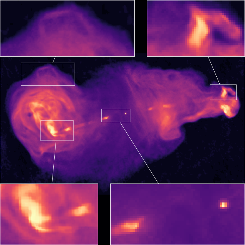
(a)

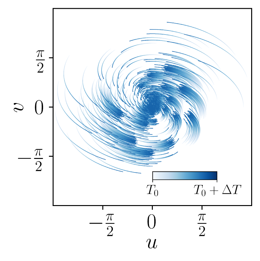
(b)

(c)

Figure 1: Illustration of a simulated RI imaging problem. (a) shows a groundtruth radio galaxy, displayed in logarithmic scale. (b) shows the sampled points in the Fourier domain. At each time $T_{0}\leq t\leq T_{0}+\Delta T$, each pair of antennas samples a single point, during a total acquisition time $\Delta T$. As the acquisition time increases, the locus of the points moves in the Fourier domain due to the Earth’s rotation. The colorbar illustrates this effect. (c) shows the measurements in the image domain.

In the context of RI imaging specifically, the current state-of-the-art SARA family of algorithms relies on optimisation algorithms solving minimization problems leveraging compressed-sensing arguments [16, 15, 17]. However, these methods are computationally demanding and their usage remains limited in the RI imaging community, favouring faster but significantly less precise CLEAN algorithms [18, 19, 20, 21]. In [22], we introduced AIRI, a class of convergent PnP algorithms, relying on a forward-backward backbone with dynamic range-specific denoisers trained on highly pre-processed unrelated optical astronomy images. This PnP approach has shown promising results in RI imaging, improving over their optimisation counterpart in terms of speed and quality, both in simulated and real RI imaging settings [22, 23].

In this article, we extend on our previous work [22] by (i) proposing a version of the PnP AIRI algorithm solving a constrained variational inclusion; (ii) introducing a new dataset for training denoisers containing high dynamic-range MRI images; (iii) quantifying the uncertainty related to the trained denoiser in the reconstructed images.

Our results show that adopting a constrained approach improves reconstructions over the current state-of-the-art, and that the proposed PnP algorithm is robust to the nature of images present in the training dataset. In particular, we show that our denoisers can be trained on MRI images and still perform well at test time on radio images, in simulated and real data settings. Finally, we show that training several denoisers allows the definition of a meaningful metric for quantifying model-based uncertainty in the reconstructions.

II Convergent PnP algorithms

In this section, we briefly review traditional tools from optimization theory and introduce PnP algorithms; we next present the proposed approach for ensuring convergence of PnP algorithms.

II-A From splitting to PnP algorithms

When adopting a variational approach, the ill-posed problem (1) is relaxed to a well-posed problem where the sought image solution is assumed to satisfy both a good fit to the measurements, as well as some prior image model (such as smoothness or sparsity). Concretely, these relaxations take the form

$$\text{find }\widehat{x}\text{ s.t. }\quad 0\in\partial f(H\widehat{x})+A(\widehat{x}),$$ (2)

where $f\colon\mathbb{R}^{M}\to\mathbb{R}$ is a convex lower semicontinuous function, $\partial\,\cdot$ denotes its subdifferential, and $A\colon\mathbb{R}^{N}\to 2^{\mathbb{R}^{N}}$ is a maximally monotone operator (MMO). We say that an operator $A\colon\mathbb{R}^{N}\to 2^{\mathbb{R}^{N}}$ is monotone if for all $(u,v)\in\mathbb{R}^{N}\times\mathbb{R}^{N}$, one has $\langle Au-Av,u-v\rangle\geq 0$; we say that $A$ is maximally monotone if it is monotone and it is not properly contained in another monotone operator [4]. In (2), the term $f\circ H$ encodes the fit of the sought image to the measurements, while the operator $A$ encodes the desired visual properties of the sought image.

In the case where $f$ is differentiable, i.e. $\partial f=\{\nabla f\}$, a celebrated algorithm for solving (2) is the forward-backward (FB) splitting algorithm, written as

$$x_{k+1}=\operatorname{D}(x_{k}-\gamma\nabla(f\circ H)(x_{k})),$$ (3)

where $\gamma$ is a stepsize, and $\operatorname{D}$ is the resolvent of $\gamma A$ (i.e. $\operatorname{D}=J_{\gamma A}$). Under the assumption that $\gamma$ is small enough, the sequence $(x_{k})_{k\in\mathbb{N}}$ can be shown to converge to a solution of (2).

In the case where $f$ is not differentiable, i.e. $\partial f\neq\{\nabla f\}$, one needs to resort to slightly more complex algorithms than (3). In this setting, an algorithm fully leveraging the structure of (2) is the primal-dual (PD) algorithm [24], written as

$$x_{k+1} =\operatorname{D}(x_{k}-\gamma H^{*}u_{k})$$ (4)

$$u_{k+1} =J_{\sigma\partial f^{*}}(u_{k}+\sigma H(2x_{k+1}-x_{k})),$$

where $f^{*}$ denotes the Legendre-Fenchel conjugate of $f$, $\operatorname{D}=J_{\gamma A}$, and where $\gamma$ and $\sigma$ are stepsizes. As before, under suitable assumptions on $\gamma$ and $\sigma$, the sequence $(x_{k})_{k\in\mathbb{N}}$ can be shown to converge to a solution of (2).

It thus appears that the prior model, which is encoded in $A$ in (2), only percolates through the resulting algorithms at the level of the operator $\operatorname{D}$.

A special case of interest is that where $A$ is a subdifferential, i.e. $A=\partial r$ for some convex function $r$. In this case, problem (2) corresponds to the minimisation problem $\widehat{x}=\underset{x}{\operatorname{argmin}}\,f(x)+r(x)$, and the resolvent of $\partial r$ coincides with the proximity operator of $r$:

$$\operatorname{D}=J_{\partial r}(y)=\operatorname{prox}_{r}(y)\overset{\text{def}}{=}\underset{u}{\arg\min}\frac{1}{2}\|u-y\|+r(u).$$ (5)

In their seminal paper introducing Plug-and-Play (PnP) algorithms [9], the authors noticed that replacing the resolvent operator by a Gaussian denoiser enabled improvements of the results compared to traditional handcrafted priors. This has since then been confirmed by a number of recent works leveraging the power of deep neural networks (DNNs) for denoising [10, 11, 13].

II-B Convergence of PnP algorithms

Despite impressive reconstruction results, PnP algorithms do not converge and can behave in an unstable manner when no additional assumption is made on the denoiser $\operatorname{D}$ [13, 14]; In this work, we follow the approach proposed in [14] which aims at enforcing $\operatorname{D}$ to behave as a resolvent. More precisely, we enforce firm nonexpansiveness of $\operatorname{D}$ by ensuring that $2\operatorname{D}-\operatorname{Id}$ is 1-Lipschitz, which ensures the existence of a maximally monotone operator $A$ such that $\operatorname{D}=J_{A}$ [4]. As a consequence, algorithms (3) and (4) converge to a point satisfying (2) with $A=\gamma^{-1}\widetilde{A}$, for some maximally monotone operator $\widetilde{A}$ [25, Theorem 3].

In order to enforce firm nonexpansiveness of $\operatorname{D}$, the training loss of the denoiser $\operatorname{D}$ is regularised with a term penalising the spectral norm of the Jacobian of $2\operatorname{D}-\operatorname{Id}$, which serves as an estimate for $\operatorname{Lip}(2\operatorname{D}-\operatorname{Id})$, as was done in [14]. More precisely, given a dataset of clean images $(x_{s})_{0\leq s\leq S}$, the denoiser $\operatorname{D}_{\theta}$ with learnable parameters $\theta\in\mathbb{R}^{P}$ is trained to solve the problem

$$\underset{\theta\in\mathbb{R}^{P}}{\text{argmin}}\,\frac{1}{S}\sum_{s=1}^{S} \|\operatorname{D}(x_{s}+\sigma w_{s})-x_{s}\|_{1}$$ (6)

$$+\lambda\operatorname{max}\{\|\operatorname{Jac}(2\operatorname{D}-\operatorname{Id})(\widetilde{y}_{s})\|,1-\epsilon\}.$$

where $x_{s}+\sigma w_{s}$ is a noisy version of $x_{s}$, with $w_{s}$ a realisation of white Gaussian noise with zero mean and variance 1, and $\sigma>0$. Furthermore, in (6), $\operatorname{Jac}(f)(x)$ denotes the Jacobian of the function $f$ computed in $x$; $\lambda>0$ is a regularisation parameter, and $\epsilon>0$ is a small parameter enforcing that $\|\operatorname{Jac}(2\operatorname{D}-\operatorname{Id})(\widetilde{y}_{s})\|\leq 1$. Eventually, similarly to [14], we compute the Jacobian at $\widetilde{y}_{s}$ which is a point sampled uniformly at random on the segment $[x_{s},y_{s}]$.

II-C Related works

We note that similar approaches have been proposed in the literature. In [26, 27], the authors adopt a similar regularisation to the one we are proposing to ensure convergence of the PnP algorithm, but they further rely on a differentiable DNN that allows explicit computation of an associated loss function. Other approaches have been proposed in the literature for controlling the stability of PnP algorithms [13, 14, 28, 26, 27, 29, 30] but they fall beyond the scope of the current article. While the original work and a large part of the PnP literature [9, 11] focused on the ADMM splitting algorithm [31], such procedures can be applied to any proximal splitting algorithm, and in particular, as will be of interest in this work, to the PD algorithm. We stress that the PnP variant of the PD algorithm has been used in a number of works [32, 10, 33, 34].

III Proposed methodology

In this section we detail our approach for training the denoisers that will be plugged in algorithms (3) and (4).

III-A Constrained and unconstrained approaches

In this paper, we aim at comparing the use of unconstrained and constrained formulations of the PnP setting for RI imaging. In the unconstrained formulation, motivated by maximum-a-priori estimation under Gaussian noise assumption, we choose

$$f(x)=\frac{1}{2\eta^{2}}\|Hx-z\|^{2}.$$ (7)

Such a choice for $f$ corresponds to the most common one in PnP algorithms. In this case, since $f$ is differentiable, the PnP-FB algorithm can be used.

Motivated by compressed-sensing theory, another popular strategy for solving (1) when the sought solution is sparse (i.e. in radio astronomy) involves using a constrained data-fidelity term. In this case,

$$f(x)=\iota_{\mathcal{B}(z,\varepsilon)}(Hx),$$ (8)

where $\iota_{\mathcal{B}(z,\varepsilon)}(\cdot)$ denotes the indicator function of $\mathcal{B}(z,\varepsilon)$, the $\ell_{2}$ ball of radius $\varepsilon$ and centred in $z$. Since $f$ is not differentiable, the FB algorithm (3) cannot be applied, but the PD algorithm (4) offers an alternative.

While the two choices for $f$ lead to different algorithms and different problems (2), they lead to the same solution for the same $A$ if the hyperparameters of the problem are chosen appropriately. However, setting the hyperparameter $\varepsilon$ in (8) is often easier than tuning the regularisation of an unconstrained formulation. In the case of Gaussian noise for $n$ in (1) for instance, $\varepsilon$ corresponds to the variance of a chi-squared distribution, that can be computed from the (rather easily estimated) standard deviation of the Gaussian noise in the measurements. Furthermore, algorithms relying on the constrained formulation have been shown to outperform their unconstrained counterparts [22]. Algorithm (3) with AIRI denoisers plugged in is abbreviated as unconstrained AIRI (uAIRI). In contrast, algorithm (4) with AIRI denoisers plugged in is abbreviated as constrained AIRI (cAIRI).

III-B Generating synthetic high dynamic range images

In the absence of clean RI image datasets, we proposed in [22] to generate a dataset of synthetic RI images to serve as a basis for training PnP denoisers as well as end-to-end DNNs to solve the inverse problem (1). A distinctive characteristic of radio images is their high dynamic range, where we define the dynamic range of an image as the ratio between its brightest and faintest non-zero pixels. While for 8-bit encoded natural images this ratio is of the order of $1/(1/255)=255$, for radio images, this value is typically $\gtrsim 10^{4}$. We stress that this is not a result of the encoding strategy of the measurements, but a characteristic of radio images, where some important features in radio images tend to have very faint intensity (for instance radio plumes or radio relics, see [35, 36]). As a consequence, radio images are usually displayed in logarithmic scale. In the remainder of this work we will use the following explicit transform $\operatorname{rlog}_{a}(x)=x_{\text{max}}\log_{a}(ax/x_{\text{max}}+1)$, which maps an image $x$ with dynamic range $a\gg 1$ and pixel values in $[x_{\text{max}}/a;x_{\text{max}}]$ to a low-dynamic range image $\operatorname{rlog}_{a}(x)$, with dynamic range $\log_{a}(2)$ and pixel values in the range $[x_{\text{max}}\log_{a}(2);x_{\text{max}}]$.

To simulate high dynamic range images, we apply the inverse of $\operatorname{rlog}_{a}$ to the images of interest. Denoting this inverse $\operatorname{rexp}_{a}$ defined as

$$\operatorname{rexp}_{a}\colon u\mapsto u_{\text{max}}(a^{u/u_{\text{max}}}-1)/a,$$ (9)

one can show that $\operatorname{rexp}_{a}$ increases the dynamic range of its input argument for sufficiently large values of $a$. In this work, we consider image datasets with maximum intensities at $1$, thus we will always assume $x_{\text{max}}=u_{\text{max}}=1$.

Applying this transform to a dataset of astronomical images acquired with optical telescopes yielded a dataset of synthetic high dynamic range radio-astronomical images.

In order to investigate the influence of the nature of the images used in the training of the denoiser, we simulate a dataset of MRI images with similar dynamic range to that of RI images. The second dataset we study in this article contains MRI images extracted from the fastMRI single-coil knee images [6], where patches of each image are combined in order to break symmetries and to increase image size. This exponentiation strategy allows us to generate 5000 MRI images of size 512$\times$512 with high dynamic range. Both the astronomical images and the MRI images were preprocessed with a blind image restoration network (SCUNet [37]) to remove noise and artefacts prior to exponentiation.

We show in Figure 2 the overall proposed preprocessing strategy on both datasets. While the semantic content of images strongly differs between the two datasets, they show similar dynamic range. Furthermore, when the denoisers plugged in a PnP algorithm are trained on the preprocessed Optical Astronomy Image Dataset, we add the OAID mention, while we add the MRID mention when they are trained on the preprocessed MRI Dataset.

	OAID	MRID
Raw	​	​
	(a)	(b)
Preprocessed	​	​
	(c)	(d)
Exponentiated	​	​
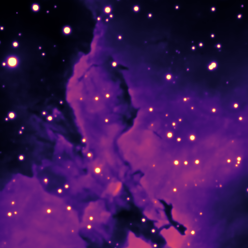
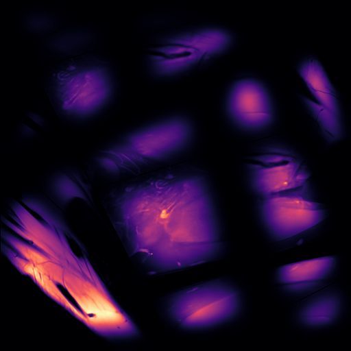
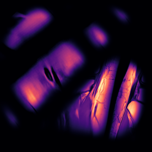
	(e)	(f)

Figure 2: The different preprocessing steps of our optical astronomy image dataset (OAID; left) and MRI dataset (MRID; right). (a) and (b) show raw images; (c) and (d) show images preprocessed with a SCUNet and the soft-thresholding removing the background; (e) and (f) show images after exponentiation. For images in MRID, concatenation and random transformation are also applied to increase image size and to break symmetries as discussed in section III-B

III-C Dynamic range estimation and network selection

The performance of PnP algorithms strongly depends on the choice of the training noise level $\sigma$ in (6) [10, 14, 38]. Since the maximum pixel intensities of the images in the training dataset have been normalised to $1$, the value $\sigma$ defines the inverse of the dynamic range for training. A heuristic rule to choose this value has been established [22], which consists of setting it equal to the inverse of signal-to-noise ratio of the observed data, itself informing the target dynamic range of the reconstruction. The inverse of signal-to-noise ratio of the observed data can be estimated from the properties of $H$ and $e$ in (1) as:

$$\sigma_{\text{heu}}=\frac{\eta}{\alpha\sqrt{2\|H\|^{2}}},$$ (10)

where we recall that $\eta$ is the standard deviation of $e$ in (1), and $\alpha$ is the maximum pixel intensity in $\overline{x}$.

Denoting by $\sigma_{0}$ the minimum (non-zero) intensity of features in the preprocessed dataset, we follow the approach of [22] for linking the exponentiation factor $a$ with the training noise level in (9). In a nutshell, this strategy amounts to equating the faintest intensity in the exponentiated image, that is $(a^{\sigma_{0}}-1)/a$, to the training noise level $\sigma$. This yields the following equation to be solved for $a$, given the faintest intensity $\sigma_{0}$ in the clean training dataset and the training noise level $\sigma$:

$$(a\sigma+1)^{1/\sigma_{0}}-a=0.$$ (11)

We thus propose to solve this equation numerically for the exponentiation parameter $a$ at different training noise levels we aim at using in our experiments. The $\sigma_{0}$ is selected such that the intensities of $1\%$ non-zero pixels in the corresponding dataset are below this value.

Unfortunately, the value of $\alpha$ cannot be easily estimated from the measurements $z$. Besides, the operator $H$ varies for each observation in our application, yielding the necessity to train a single denoiser for each observation if one wants to apply (10) rigorously. Building on [22, 39] we propose to train a shelf of denoisers with different noise levels, and to estimate the dynamic range of $\overline{x}$ on the fly while running the PnP algorithm. More precisely, the denoisers are trained in advance for 8 noise levels covering the full range of possible dynamic ranges of interest for a class of radio observations. During the PnP reconstruction process, the maximum intensity of the back-projected image is used as the initial estimate $\alpha$, marked as $\widetilde{\alpha}$. Then, the network $\operatorname{D}_{\sigma}$ will be chosen where $\sigma$ is the closest training noise level below $\sigma_{\text{heu}}$ which is calculated with $\widetilde{\alpha}$. The activation of the denoiser is thus rescaled with a factor $\beta=\widetilde{\alpha}\sigma_{\text{heu}}/\sigma$ as

$$\operatorname{D}(\cdot)=\beta\operatorname{D}_{\sigma}(\cdot/\beta),$$ (12)

ensuring both that the input to the network has maximum intensity of $1$ and that the effective standard deviation of the residual noise in the input to the denoiser trained with noise level $\sigma$ matches the heuristic (10).

In practice, the peak value of the back-projected image is a loose upper bound estimation of the real peak value. To solve the inaccurate estimation of $\sigma_{\text{heu}}$, we estimate $\widetilde{\alpha}$ as the maximum intensity of the reconstructed image at each iteration of the PnP algorithm. The value of $\sigma_{\text{heu}}$ is monitored at each iteration to check whether $\operatorname{D}_{\sigma}$ and the scaling factor $\beta$ need to be updated.

III-D Denoiser realisation and model uncertainty quantification

If obtaining an estimate of the solution to a specific model is desirable, it is also of interest to be able to quantify the uncertainty in the recovered solution; this is all the more important in applications such as RI imaging where only very few features of the image can be measured [40]. In practice, this uncertainty quantification is often performed by sampling from the posterior linked to $A$ in (2), e.g. with MCMC methods [41, 42], but other strategies have been proposed [40, 43, 44]; in a nutshell, these methods aim at quantifying the aleatoric uncertainty induced by the measurement procedure (1) in the reconstructed image.

Similarly to [45], we instead propose in this work to investigate the epistemic uncertainty in the reconstruction, induced by variations in the denoiser $\operatorname{D}$ (and thus implicitly in the regularisation model characterised by $A$). In fact, while the choice of $A$ in (2) is a cornerstone of the reconstruction quality, its relationship with the denoiser $\operatorname{D}$ in the case of PnP algorithms remains unclear since no closed form for $A$ is available in general, not to mention the high number of parameters and the (by nature) imperfect training procedure of $\operatorname{D}$.

Training the same architecture $\operatorname{D}$ for the same task but in different settings (i.e. with different initialisation, Gaussian noise realisation or patch selection) leads to networks $\operatorname{D}$ with different weights, but consistent denoising performance. In turn, these different denoiser realizations yield distinct prior realizations. More precisely, assume that we train $Q\in\mathbb{N}$ denoisers $(\operatorname{D}_{q})_{1\leq q\leq Q}$ with (6), and that the sole difference between these denoisers arises from distinct random realizations influencing their training process. These denoisers yield unique monotone operators $(A_{q})_{1\leq q\leq Q}$, and plugging $\operatorname{D}_{q}$ within the PnP algorithms (3) and (4) returns $\widehat{x}_{q}$ satisfying (2). This procedure gives us a set of solutions $\operatorname{Sol}=\{\widehat{x}_{1},\ldots,\widehat{x}_{Q}\}$ to each problem (1); in turn, the (pixel-wise) empirical standard deviation of $\operatorname{Sol}$ yields an estimator of the epistemic uncertainty [46].

Similar approaches to ours were proposed in [47, 45]. In particular, the unfolded algorithm from [45] also yields a set of estimates $\operatorname{Sol}$; the authors however train a single model the weights of which can be sampled, while we train a set of denoisers in a traditional fashion, and in their case, no link to a variational inclusion problem (2) can be made. We note that previous works have studied aleatoric and epistemic uncertainties in the context of end-to-end supervised learning with Bayesian neural networks [48, 49, 50, 51, 52, 53].

IV Experimental results on simulated data

In this section, we show the performance of different algorithms for reconstructing RI images from simulated observations.

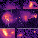
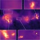
(a) Groundtruth	(b) Back-projection	(c) CLEAN	(d) UNet	(e) uSARA	(f) SARA
		$(5.45,7.07)$	$(17.02,7.42)$	$(24.55,24.90)$	$(27.74,25.16)$
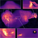
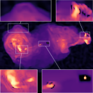
(g) uPnPBM3D	(h) cPnPBM3D	(i) uAIRIMRID	(j) cAIRIMRID	(k) uAIRIOAID	(l) cAIRIOAID
$(20.45,24.00)$	$(22.34,24.41)$	$(26.46,25.27)$	$(27.76,25.10)$	$(26.49,25.78)$	$(28.66,26.28)$

Figure 3: Results of various algorithms for the RI imaging problem. Top left image (a) shows the groundtruth image, (b) shows the simulated measurements back-projected in the real image domain. Other images show reconstructions with different imaging algorithms; (SNR, logSNR) metrics associated with each reconstruction are shown beneath each image. All images are displayed in logarithmic scale (see colorbar on the right).

IV-A Test dataset and evaluation metrics

Our test dataset consists of 3 radio images (3c353, Hercules A, and Centaurus A, see [22] for more details) of size $N=$ 512$\times$512. Each image has the peak value normalised to 1, and a dynamic range slightly above $10^{4}$. For each image, we generate 4$\times$5 RI measurement vectors from different operators $H$ as (1). Each operator $H$ corresponds to a simulated MeerKAT telescope [54] acquisition with specific pointing direction and observation time. We consider five distinct pointing directions chosen at random, and for each direction, we vary the observation time with $\Delta T$ selected from the set $\{1\text{h},2\text{h},4\text{h},8\text{h}\}$. This leads to a total of 4$\times$5 inverse problems for each groundtruth image, i.e. a total of 4$\times$15 inverse problems with $z\in\mathbb{C}^{M}$ containing $M\in\{4\times 10^{5},8\times 10^{5},1.6\times 10^{6},3.2\times 10^{6}\}$ data points, each value of $M$ being related to a value of $\Delta T$. Figure 1 (b) shows one of the test sampling patterns for a given pointing direction and observation time $\Delta T=4\text{h}$. The dynamic ranges of all the measurements fall in the range $[2.5\times 10^{3},1.4\times 10^{4}]$, and the average dynamic range of the measurements with $\Delta T=1,2,4,8$ are $2.9\times 10^{3}$, $3.9\times 10^{3}$, $5.6\times 10^{3}$ and $1.1\times 10^{4}$ respectively.

We evaluate the reconstruction accuracy with the SNR and logSNR metrics. Recall that, given a groundtruth image $\overline{x}$ and an estimated image $\widehat{x}$, the reconstruction SNR is defined as $\operatorname{SNR}(\overline{x},\widehat{x})=20\log(\|\overline{x}\|/\|\overline{x}-\widehat{x}\|)$. In order to evaluate the performance of the algorithms at very faint intensities (high dynamic range), we also consider the logSNR metric [22] writing $\operatorname{logSNR}(\overline{x},\widehat{x})=\operatorname{SNR}(\operatorname{rlog}_{a}(\overline{x}),\operatorname{rlog}_{a}(\widehat{x}))$. The images in this article are presented in a logarithmic scale, i.e. for an image $x$, visualizations show $\operatorname{rlog}_{a}(x)$. The values of $a$ in $\operatorname{rlog}_{a}(\cdot)$ should ideally be set to the corresponding dynamic range of each measurement. For the $\operatorname{logSNR}$ metric, we set $a=2.5\times 10^{3}$, the lowest dynamic range of all the synthetic measurements across $\Delta T=1,2,4,8$. Choosing a single value for $a$ preserves the consistency of the $\operatorname{logSNR}$ metric across different reconstructions and $\Delta T$s. For the visualisation of images, a value of $a=10^{4}$ is chosen, more representative of the dynamic range values for the $\Delta T=4,8$ cases displayed. Given $Q$ trained models, the model uncertainty is estimated using the empirical standard deviation (std) metric, defined as $\operatorname{std}(\operatorname{Sol})=1/\sqrt{Q-1}\sum_{q=1}^{Q}|\widehat{x}_{q}-\operatorname{mean}(\operatorname{Sol})|$. Additionally, we calculate the mean-over-standard deviation (std/mean) ratio, defined as $\operatorname{std/mean}(\operatorname{Sol})=\operatorname{std}(\operatorname{Sol})/\operatorname{mean}(\operatorname{Sol})$, to compare the uncertainty for features with different intensities.

IV-B Benchmark algorithms

We compare the performance of the proposed algorithms with several other methods: CLEAN [20], a matching-pursuit algorithm which is the reference algorithm in the RI imaging community and is thus considered a meaningful baseline; a UNet [11] that was trained on the proposed synthetic datasets to solve the RI imaging problem in a supervised end-to-end fashion for each $\Delta T$; and the Sparsity Averaging Reweighted Analysis approaches uSARA [22] and SARA [17], which are, respectively, slightly evolved versions of the traditional FB (3) and PD algorithms (4), leveraging a redundant wavelet dictionary to impose simultaneous sparsity in multiple wavelet bases and a reweighting procedure to account for a nonconvex log-sum prior. uSARA and SARA have been exhaustively validated for RI imaging, where they have defined new state-of-the-art.

We further test our algorithms with the BM3D denoiser [55] in (3) and (4) instead of the proposed trained denoiser. We stress that BM3D is a non-trained denoiser, which allows circumventing the lack of training data in RI imaging; however, it does not yield convergent PnP algorithms and suffer from slow inference time. The algorithm with a BM3D denoiser plugged into (3) is named uPnP_BM3D and the one with BM3D plugged into (4) is named cPnP_BM3D.

IV-C Training details

We use the DnCNN network architecture [56] with the same additional changes as in [22], i.e. all batch normalization layers are removed, ReLU layers are replaced by leaky ReLU layers, and an additional ReLU is added to ensure positivity of the reconstructed image.

We train a shelf of denoisers for 8 noise levels covering the full range of possible dynamic ranges of interest. Each denoiser is trained on both optical astronomy and MRI datasets with the training loss (6) on randomly cropped patches of size 49$\times$49. Each training pair $(x_{s},y_{s})_{0\leq s\leq S}$ is generated on the fly, with $x_{s}=\operatorname{rexp}_{a}(x_{s}^{\text{patch}})$ where $x_{s}^{\text{patch}}$ is the randomly cropped patch in the synthetic dataset, and $a$ is chosen as per (11). The value of the regularisation parameter $\lambda$ in (6) enforcing stability of the PnP algorithm is fine tuned for each denoiser. Training is performed for 5000 epochs with the Adam algorithm [57], with gradients clipped at $10^{-2}$. The learning rate is divided by 2 every 900 epochs. Following [22], we named the denoisers trained with the non-expansiveness term for RI imaging as AIRI denoisers.

We choose the following 8 training noise levels for our shelf: $\{2.5\times 10^{-6},5.0\times 10^{-6},1.0\times 10^{-5},2.0\times 10^{-5},4.0\times 10^{-5},8.0\times 10^{-5},1.6\times 10^{-4},3.2\times 10^{-4}\}$. As a consequence, this strategy ensures that $\sigma_{\text{heu}}/\sigma\in[1,2]$ in (12).

IV-D Results for image estimation

Visual results for $\Delta T=8\text{h}$ are shown in Figure 3. We first observe that the CLEAN algorithm yields highly blurred and noisy reconstructions. As was observed in [22], the UNet recovers the high intensity results rather well, but struggles at lower intensities (see the extended purple areas): this translates in a relatively good SNR metric, but lower logSNR. Optimisation methods uSARA and SARA show faithful reconstructions, despite noticeable wavelet artefacts around the central point source which is challenging to recover for all algorithms. While no significant difference between the two methods can be noticed in logarithmic scale, we stress that uSARA struggles to recover the high intensity values correctly, which translates in a lower SNR than its constrained counterpart, SARA. BM3D based PnP algorithms (i.e. uPnP_BM3D and cPnP_BM3D) show horizontal and/or vertical artefacts. PnP algorithms with the proposed denoisers (uAIRI and cAIRI) show better reconstruction qualities than other methods, with no significant difference between each method. However, the unconstrained PnP algorithms (3) do not recover high intensities as well as their constrained counterparts (4). This is in line with the results obtained with uSARA and SARA. Interestingly, visual results of OAID and MRID AIRI algorithms are very similar up to small additional artefacts for MRID.

Figure 4 gives the average SNR and logSNR metrics of reconstructions estimated with various algorithms. On these plots, each point is an average over the 15 inverse problems considered for each observation time, error bars representing the 95% confidence intervals. Both uSARA and SARA optimisation algorithms significantly outperform the baseline CLEAN algorithm and the UNet for the two considered metrics. AIRI algorithms improve by 1 to 2 dB over their pure optimisation counterparts uSARA and SARA. In each case (both PnP and pure optimisation), the constrained approach performs better than the unconstrained one, particularly on the SNR metric. We explain this phenomenon by the good ability of constrained methods to recover high intensity values after fewer iterations than their unconstrained counterparts.

Figure 4: Reconstruction metrics on the simulated data experiments for different imaging algorithms. Leftmost plots show the metrics for baseline algorithms, namely the UNet and CLEAN. Center (resp. right) plot shows metrics as a function of the observation time for reconstructions obtained with the unconstrained (3) (resp. the constrained (4)) algorithms. Top row gives SNR metrics; bottom row gives logSNR metric. Each point is an average value over 15 inverse problems; shaded areas represent the 95% confidence intervals.

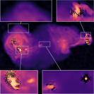
(a) Adaptive Peak	(b) Exact Peak	(c) Dirty Peak
$(26.46,25.27)$	$(26.48,25.27)$	$(2.80,12.78)$

Figure 5: uAIRI_MRID reconstructions of the same simulated measurement in Figure 3 with different image peak value $\alpha$ estimation schemes: (a) Adaptive peak value estimation (b) Using the exact peak value of the groundtruth (1.00) (c) Using the maximum intensity of the back-projected image (61.18); (SNR, logSNR) metrics associated with each reconstruction are shown beneath each image.

In Table I, we give the computational time of the denoising step for different denoisers. When executed on a GPU, AIRI denoisers demonstrate a 20-fold increase in inference speed compared to the proximity operator in SARA. Conversely, the BM3D algorithm exhibits slow inference, raising doubt on its practicality in iteration intensive algorithms, such as ours. These results underscore the efficiency of DNN-based denoisers, benefiting seamlessly from GPU acceleration.

	AIRI (GPU)	AIRI (CPU)	SARA	BM3D
Time (s.)	0.05 $\pm$ 0.02	7.92 $\pm$ 0.52	1.31 $\pm$ 1.12	15.08 $\pm$ 0.40

TABLE I: Average time (in seconds) taken by the denoising step for solving 60 simulated inverse problems with different denoisers $\operatorname{D}$ when plugged in (3).

In section III-C, we showed that the peak intensity estimation of the target image affects the choice of the optimal denoising network $\operatorname{D}_{\sigma}$ and the corresponding scaling factor $\beta$ in the uAIRI and cAIRI algorithms. In our simulated experiments, the true peak value in the sought reconstructed image is known (it is equal to 1) and the peak value of the back-projected images vary from 30 to 68 for different measurements. To prove the feasibility of the proposed adaptive peak estimation scheme, we ran the simulated experiments with $\alpha$ set to the exact maximum intensity of the groundtruth image and the maximum intensity of the back-projected image while keeping all other settings the same. Some visual results are shown in Figure 5, demonstrating that the proposed adaptive peak estimation scheme yields reconstructions with the same quality as if the true peak value were known. We also found that if the estimated peak value differs too much from the real peak value, like the situation in Figure 5(c), reconstructions may suffer from chess-board artefacts in the high intensity region. We attribute this suboptimality to the fact that the denoisers are applied to images with peak value far below 1, a range for which they have not been trained.

IV-E Robustness to denoiser realisation and model uncertainty

In order to investigate the robustness of the proposed approach and following the discussion from Section  III-D, we trained $Q=15$ denoisers per training dataset (i.e. OAID and MRID) in the same experimental conditions, but with different random seeds generating the (pseudo) random processes involved during training. This impacts both the initialisation of the denoisers (each being initialised with a different random state) and the random image patches presented to the networks during training, as well as the Gaussian random noise generated in (6). We next plug each denoiser in algorithms (3) and (4). This yields two sets of solutions $\operatorname{Sol}$ of 15 elements, one per training datasets; see Section III-D for more details.

Figure 6 shows visual results for algorithms (3) and (4) with different denoisers realisations. We notice that the reconstructions from each random seed, as well as the mean image, show no clear difference, except around the point source at the centre of the image. The mean-over-standard deviation map shows the ratio in the region where the mean pixel intensity is higher than the estimated noise level given by (10). Overall, the empirical standard deviation is small in comparison to the estimated intensity ($\lessapprox 10\%$ of the mean intensity), except around the centre source, where the standard deviation reaches $20\%$ of the mean intensity. This observation is all the more interesting as the central source estimation is often unsatisfying, most algorithms hallucinating a black ring around it.

cAIRIOAID
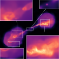
	(a) $\widehat{x}_{1}$	(b) $\widehat{x}_{2}$	(c) $\widehat{x}_{3}$
	$(27.15,25.49)$	$(27.45,24.87)$	$(27.21,24.70)$
cAIRIOAID
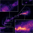
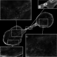
	(d) mean image	(e) std. image	(f) std/mean
	$(27.86,25.11)$
uAIRIOAID
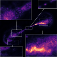
	(g) mean image	(h) std. image	(i) std/mean
	$(27.69,25.45)$
cAIRIMRID
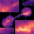
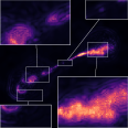
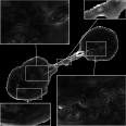
	(j) mean image	(k) std. image	(l) std/mean
	$(27.45,25.87)$
uAIRIMRID
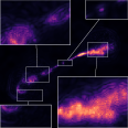
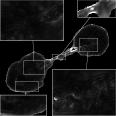
	(m) mean image	(n) std. image	(o) std/mean
	$(27.45,26.31)$

Figure 6: Sensitivity of the imaging result to the training conditions of the denoiser realisation. (a)-(c) show image reconstructions with cAIRI_OAID for 3 denoisers, each trained with a different random seed. (d)-(f) show the mean image, standard deviation and mean-over-standard deviation maps for reconstructions obtained with 15 networks trained on the astronomical dataset and plugged in the cAIRI_OAID algorithm; next rows show the same results but obtained with other AIRI variants.

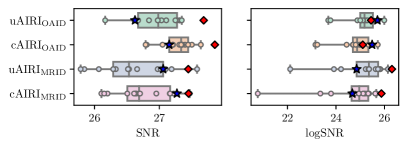
Figure 7: Results for 15 different runs of the uAIRI and cAIRI algorithms for simulated measurements with $\Delta T=4$h. The red diamond indicates the reconstruction metric of the mean image of the 15 reconstructions; the blue star indicates the models that are used in our deterministic experiments (in Figure 3 and 4).

Figure 7 displays the reconstruction metrics for 15 denoiser realisations in the context of a single inverse problem at $\Delta T=4\text{h}$, with selected samples depicted in Figure 6. The reconstruction quality offered by different denoiser realisations spans about 1.5dB in SNR and 4dB in logSNR. Notably, the variations in SNR and logSNR metrics among the reconstructed images, as shown in Figure 6, are not readily discernible at the image level.

In general, uAIRI tends to provide better logSNR metrics than cAIRI, while the opposite holds for SNR. Furthermore, reconstructions produced with cAIRI_OAID and cAIRI_MRID exhibit less variation in SNR compared to those generated with uAIRI_OAID and uAIRI_MRID. Interestingly, the SNR of both the mean images is slightly higher than the mean SNR, indicating that the mean image offers enhanced fidelity. Yet, computing this image necessitates multiple denoiser realizations and algorithm runs.

As the overall variation in reconstruction quality remains small, these results suggest that our AIRI PnP algorithms are resilient to modest variations inherent to the training process.

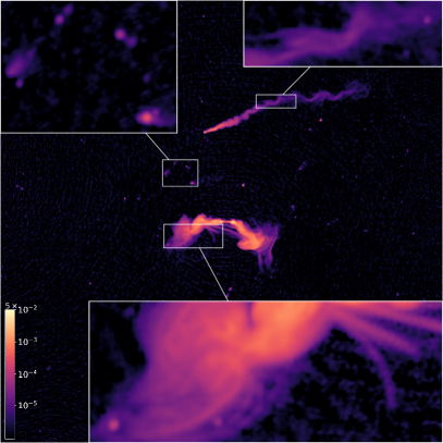
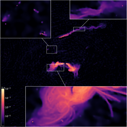
(a) Baseline (CLEAN)	(b) Proposed (cAIRIOAID)

Figure 8: Imaging of a wide field of view (image size is 2560$\times$2560) containing the ESO 137-006 galaxy and other radio sources of interest from data acquired with the MeerKAT telescope. (a) imaging result with the baseline CLEAN algorithm; (b) imaging result with the proposed cAIRI_OAID algorithm.

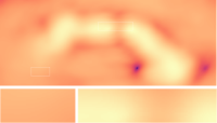
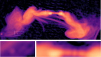
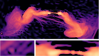
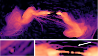
(a) Back-projected image	(b) CLEAN	(c) uSARA	(d) SARA
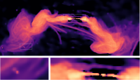
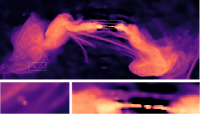
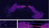
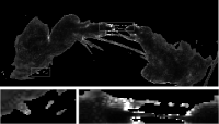
(e) cAIRIOAID	(f) Mean cAIRIOAID	(g) Std cAIRIOAID	(h) Std/mean cAIRIOAID
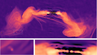
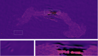
(i) cAIRIMRID	(j) Mean cAIRIMRID	(k) Std cAIRIMRID	(l) Std/mean cAIRIMRID

Figure 9: Imaging of a wide field of view (image size is 2560$\times$2560) containing the ESO 137-006 galaxy. Due to the large size of the field of view (same as in Figure 8), we only display a center-crop of size 640$\times$256 over the ESO 137-006 galaxy. (a) shows the back-projected image; (b) the imaging result with the baseline CLEAN algorithm; (c) with the uSARA and (d) SARA algorithm. The white arrow in (d) points towards a filament that not all algorithms manage to recover. The two bottom rows show, from left to right a sample reconstruction with cAIRI_OAID in (e), cAIRI_MRID in (i), the mean image obtained over 15 reconstructions ((g) and (k)), and the ratio image std/mean in (h) and (l).

V Application to real astronomical data

In this section, we validate the proposed algorithms by imaging of a wide field of view containing the ESO 137-006 galaxy and other radio sources of interest, from data acquired with the MeerKAT telescope. This field of view has recently sparked interest in the radio astronomy community for the observation of collimated synchrotron threads [58]. We stress that we rely on the same shelf of denoisers that was used in the experiments on simulated data, meaning that no denoisers had to be trained specifically for the experiments in this section.

V-A Data acquisition

Unlike in the simulated case, the inverse problem formulation in real data settings is subject to both measurement noise and instrumental errors. Among other consequences, the model in (1) is subject to approximation errors, in particular at the level of the modelling of the operator $H$ which can only be approximately estimated in practice through a so-called calibration procedure [59].

The considered data were acquired by the MeerKAT telescope [54] and we use a subset of the data used in [58, 23]. More specifically, the vector $z$ in (1) consists of a concatenation of 10 frequency channels extracted from observation frequencies ranging between 961 and 1503 Hz, and the unknown target image $\overline{x}$ is of size $2560\times 2560$. The calibration procedure and data weighting scheme applied to the data are detailed in [58, 23].

V-B Imaging results

We show the full imaging field of view in Figure 8 for both the baseline CLEAN algorithm as well as the cAIRI_OAID. More reconstruction results are displayed in Figure 9. The maximum intensities of the reconstructions given by various methods are around $0.05$, which yields a dynamic range of approximately $10^{4}$. Therefore, we set $x_{\text{max}}=0.05$ and $a=10^{4}$ in the $\operatorname{rlog}_{a}(\cdot)$ for visualization. Overall, the imaging quality for all algorithms is in line with what was observed on experiments using simulated data (see Section IV). We notice that both the pure optimisation algorithms (SARA and uSARA) and the PnP algorithms significantly improve over CLEAN. However, SARA shows important wavelet artefacts which we explain by calibration errors in the estimation of $H$, and lack of good estimation of the noise standard deviation for $e$ in (1), on which SARA’s hyperparmeters rely (see [60]). Both cAIRI_OAID and cAIRI_MRID yield images with fewer artefacts than SARA and better resolution (see bottom-left zoom). Furthermore, notice that the filament shown with the white arrow in Figure 9 (d) is recovered by both cAIRI_OAID and cAIRI_MRID but not by CLEAN or uSARA. We however underline that neither are completely artefact free: the cAIRI_OAID yields reconstructions with dotted artefacts (see the filaments in Figure 9 (e)), while the cAIRI_MRID yields light ringing artefacts in the reconstruction (see the filaments in Figure 9 (i)).

As in Section IV-E, we run the proposed algorithm with 15 different denoisers and investigate the statistics of the reconstructed images. The results on denoisers trained on OAID from Figure 9 (e)-(h) show that the mean (f) is consistent with a single sample (e), and that only very mild variation occur between the different solutions to the problem, as suggested by the empirical standard deviation image (g). Furthermore, the small ratio between the standard deviation and the mean suggests that the variations in the reconstructions related to the model uncertainty are small compared to the image itself.

We observe different results for denoisers trained on MRID in Figure 9 (i)-(l). The mean image (j) shows a different background value than on the sample (i), along with stronger localized artefacts. The standard deviation map (k) suggests that different denoiser realisations can yield highly different background values in the reconstruction. The ratio map (l) suggests that these variations dominate the signal at very faint intensities.

This study suggests that models trained on the proposed synthetic astronomical dataset (OAID) are more robust than those trained on the synthetic bio dataset (MRID). In practice, we observed that some of the networks trained on the bio dataset showed unstable results when plugged in the PnP algorithm in the case of real imaging, despite the low Jacobian spectral norm of the denoisers. We did not observe such phenomenon on the synthetic dataset, and presume this might be related to the null space of the measurement operator in the higher dimensional setting faced in the current real data experiment.

VI Conclusion

In this paper, we proposed a general PnP algorithmic framework for large-scale high-dynamic range image reconstruction and model uncertainty quantification in radio astronomy. In particular, we have extended our earlier AIRI algorithm to the PDFB case to enable addressing problems with constrained data-fidelity terms. Faithful to the spirit of the PnP algorithms, both uAIRI and cAIRI algorithms fully mirror their pure-optimisation counterparts uSARA and SARA.

Our experiments suggest that cAIRI perform better than its unconstrained counterpart uAIRI, while each respectively improved on their respective pure optimisation counterparts (SARA and uSARA). Our method improves over the state-of-the-art SARA algorithm both in simulated experimental settings, and in real imaging problems. This refines the results of our earlier work, where we had pointed out the limitations of uAIRI [22]. We believe that this jump in performance is related to the high-dynamic range of the target image, where some point sources with intensities orders of magnitude higher than background pixels are better resolved with constrained algorithms.

By training a shelf of a few networks for a wide range of dynamic range of interest in RI imaging, we circumvent the necessity to retrain denoisers when applying AIRI to new imaging setups, where the measurement operator and noise levels may be different. Our work suggests that AIRI algorithms are robust to strong variations in the nature of the training dataset (MRI images versus optical astronomy images), while the capability to adapt the dynamic range of the dataset to the target dynamic range of observation, resulting in the creation of dynamic range-specific denoisers, is a critical feature of the AIRI framework.

Our experiments confirm PnP algorithms’ strong generalization abilities, adapting easily to real data without fine-tuning. In this study, we demonstrate that AIRI denoisers, despite subtle variations in parameter initialisation, noise realisation and patch selection, consistently yield very similar results when integrated into PnP algorithms. This ensemble of solutions provides an epistemic uncertainty metric for the PnP algorithm. Our results show minimal standard deviations in signal intensity for most denoiser configurations, except for those trained on MRI data. This highlights the need for further fine-tuning when applying bio-trained networks to real imaging scenarios.

Future research directions include the investigation of whether the proposed synthetic image generation procedure would extend well to other types of images, as well as the extension to other RI imaging modalities, such as multi-band imaging.

Data Availability

The utilised real data are observations with the MeerKAT telescope (Project ID SCI-20190418-SM-01). The SARA code is available with the MATLAB toolbox from the Puri-Psi webpage. The uSARA, uAIRI and cAIRI codes will become available in a later release of the Puri-Psi library for RI imaging.

References

- [1] S. Mallat, A wavelet tour of signal processing. Elsevier, 1999.
- [2] K. Bredies, K. Kunisch, and T. Pock, “Total generalized variation,” SIAM Journal on Imaging Sciences, vol. 3, no. 3, pp. 492–526, 2010.
- [3] J.-F. Cai, B. Dong, S. Osher, and Z. Shen, “Image restoration: total variation, wavelet frames, and beyond,” Journal of the American Mathematical Society, vol. 25, no. 4, pp. 1033–1089, 2012.
- [4] H. H. Bauschke, P. L. Combettes et al., Convex analysis and monotone operator theory in Hilbert spaces. Springer, 2011, vol. 408.
- [5] E. K. Ryu and W. Yin, Large-Scale Convex Optimization: Algorithms & Analyses via Monotone Operators. Cambridge University Press, 2022.
- [6] J. Zbontar, F. Knoll, A. Sriram, T. Murrell, Z. Huang, M. J. Muckley, A. Defazio, R. Stern, P. Johnson, M. Bruno et al., “fastmri: An open dataset and benchmarks for accelerated mri,” arXiv preprint arXiv:1811.08839, 2018.
- [7] T. M. Quan, T. Nguyen-Duc, and W.-K. Jeong, “Compressed sensing mri reconstruction using a generative adversarial network with a cyclic loss,” IEEE transactions on medical imaging, vol. 37, no. 6, pp. 1488–1497, 2018.
- [8] J. Liang, J. Cao, G. Sun, K. Zhang, L. Van Gool, and R. Timofte, “Swinir: Image restoration using swin transformer,” in Proceedings of the IEEE/CVF international conference on computer vision, 2021, pp. 1833–1844.
- [9] S. V. Venkatakrishnan, C. A. Bouman, and B. Wohlberg, “Plug-and-play priors for model based reconstruction,” in IEEE Global Conference on Signal and Information Processing, 2013, pp. 945–948.
- [10] T. Meinhardt, M. Moller, C. Hazirbas, and D. Cremers, “Learning proximal operators: Using denoising networks for regularizing inverse imaging problems,” in Proceedings of the IEEE International Conference on Computer Vision, 2017, pp. 1781–1790.
- [11] K. Zhang, Y. Li, W. Zuo, L. Zhang, L. Van Gool, and R. Timofte, “Plug-and-play image restoration with deep denoiser prior,” IEEE Transactions on Pattern Analysis and Machine Intelligence, vol. 44, no. 10, pp. 6360–6376, 2022.
- [12] R. Liu, Y. Sun, J. Zhu, L. Tian, and U. S. Kamilov, “Recovery of continuous 3d refractive index maps from discrete intensity-only measurements using neural fields,” Nature Machine Intelligence, vol. 4, no. 9, pp. 781–791, 2022.
- [13] E. Ryu, J. Liu, S. Wang, X. Chen, Z. Wang, and W. Yin, “Plug-and-play methods provably converge with properly trained denoisers,” in International Conference on Machine Learning. PMLR, 2019, pp. 5546–5557.
- [14] J.-C. Pesquet, A. Repetti, M. Terris, and Y. Wiaux, “Learning maximally monotone operators for image recovery,” SIAM Journal on Imaging Sciences, vol. 14, no. 3, pp. 1206–1237, 2021.
- [15] Y. Wiaux, L. Jacques, G. Puy, A. M. Scaife, and P. Vandergheynst, “Compressed sensing imaging techniques for radio interferometry,” Monthly Notices of the Royal Astronomical Society, vol. 395, no. 3, pp. 1733–1742, 2009.
- [16] E. J. Candes, J. K. Romberg, and T. Tao, “Stable signal recovery from incomplete and inaccurate measurements,” Communications on Pure and Applied Mathematics: A Journal Issued by the Courant Institute of Mathematical Sciences, vol. 59, no. 8, pp. 1207–1223, 2006.
- [17] R. E. Carrillo, J. D. McEwen, and Y. Wiaux, “Sparsity averaging reweighted analysis (sara): a novel algorithm for radio-interferometric imaging,” Monthly Notices of the Royal Astronomical Society, vol. 426, no. 2, pp. 1223–1234, 2012.
- [18] T. J. Cornwell, “Multiscale clean deconvolution of radio synthesis images,” IEEE Journal of selected topics in signal processing, vol. 2, no. 5, pp. 793–801, 2008.
- [19] A. Offringa, B. McKinley, N. Hurley-Walker, F. Briggs, R. Wayth, D. Kaplan, M. Bell, L. Feng, A. Neben, J. Hughes et al., “Wsclean: an implementation of a fast, generic wide-field imager for radio astronomy,” Monthly Notices of the Royal Astronomical Society, vol. 444, no. 1, pp. 606–619, 2014.
- [20] A. Offringa and O. Smirnov, “An optimized algorithm for multiscale wideband deconvolution of radio astronomical images,” Monthly Notices of the Royal Astronomical Society, vol. 471, no. 1, pp. 301–316, 2017.
- [21] P. Arras, H. L. Bester, R. A. Perley, R. Leike, O. Smirnov, R. Westermann, and T. A. Enßlin, “Comparison of classical and bayesian imaging in radio interferometry-cygnus a with clean and resolve,” Astronomy & Astrophysics, vol. 646, p. A84, 2021.
- [22] M. Terris, A. Dabbech, C. Tang, and Y. Wiaux, “Image reconstruction algorithms in radio interferometry: From handcrafted to learned regularization denoisers,” Monthly Notices of the Royal Astronomical Society, vol. 518, no. 1, pp. 604–622, 2023.
- [23] A. Dabbech, M. Terris, A. Jackson, M. Ramatsoku, O. M. Smirnov, and Y. Wiaux, “First AI for deep super-resolution wide-field imaging in radio astronomy: unveiling structure in eso 137-006,” The Astrophysical Journal Letters, vol. 939, no. 1, p. L4, 2022.
- [24] A. Chambolle and T. Pock, “A first-order primal-dual algorithm for convex problems with applications to imaging,” Journal of mathematical imaging and vision, vol. 40, pp. 120–145, 2011.
- [25] B. C. Vũ, “A splitting algorithm for dual monotone inclusions involving cocoercive operators,” Advances in Computational Mathematics, vol. 38, no. 3, pp. 667–681, 2013.
- [26] S. Hurault, A. Leclaire, and N. Papadakis, “Gradient step denoiser for convergent plug-and-play,” in International Conference on Learning Representations, 2022. [Online]. Available: https://openreview.net/forum?id=fPhKeld3Okz
- [27] ——, “Proximal denoiser for convergent plug-and-play optimization with nonconvex regularization,” in International Conference on Machine Learning. PMLR, 2022, pp. 9483–9505.
- [28] J. Hertrich, S. Neumayer, and G. Steidl, “Convolutional proximal neural networks and plug-and-play algorithms,” Linear Algebra and its Applications, vol. 631, pp. 203–234, 2021.
- [29] A. Repetti, M. Terris, Y. Wiaux, and J.-C. Pesquet, “Dual forward-backward unfolded network for flexible plug-and-play,” in 2022 30th European Signal Processing Conference (EUSIPCO). IEEE, 2022, pp. 957–961.
- [30] H. Y. Tan, S. Mukherjee, J. Tang, and C.-B. Schönlieb, “Provably convergent plug-and-play quasi-newton methods,” arXiv preprint arXiv:2303.07271, 2023.
- [31] S. Boyd, N. Parikh, E. Chu, B. Peleato, J. Eckstein et al., “Distributed optimization and statistical learning via the alternating direction method of multipliers,” Foundations and Trends® in Machine learning, vol. 3, no. 1, pp. 1–122, 2011.
- [32] F. Heide, M. Steinberger, Y.-T. Tsai, M. Rouf, D. Pająk, D. Reddy, O. Gallo, J. Liu, W. Heidrich, K. Egiazarian et al., “Flexisp: A flexible camera image processing framework,” ACM Transactions on Graphics (ToG), vol. 33, no. 6, pp. 1–13, 2014.
- [33] S. Ono, “Primal-dual plug-and-play image restoration,” IEEE Signal Processing Letters, vol. 24, no. 8, pp. 1108–1112, 2017.
- [34] S. K. Shastri, R. Ahmad, and P. Schniter, “Autotuning plug-and-play algorithms for mri,” in 2020 54th Asilomar Conference on Signals, Systems, and Computers. IEEE, 2020, pp. 1400–1404.
- [35] V. Missaglia, F. Massaro, A. Capetti, M. Paolillo, R. Kraft, R. D. Baldi, and A. Paggi, “Watcat: a tale of wide-angle tailed radio galaxies,” Astronomy & Astrophysics, vol. 626, p. A8, 2019.
- [36] D. Wittor, S. Ettori, F. Vazza, K. Rajpurohit, M. Hoeft, and P. Domínguez-Fernández, “Exploring the spectral properties of radio relics–i: integrated spectral index and mach number,” Monthly Notices of the Royal Astronomical Society, vol. 506, no. 1, pp. 396–414, 2021.
- [37] K. Zhang, Y. Li, J. Liang, J. Cao, Y. Zhang, H. Tang, R. Timofte, and L. Van Gool, “Practical blind denoising via swin-conv-unet and data synthesis,” arXiv preprint, 2022.
- [38] K. Wei, A. I. Avilés-Rivero, J. Liang, Y. Fu, H. Huang, and C.-B. Schönlieb, “Tfpnp: Tuning-free plug-and-play proximal algorithms with applications to inverse imaging problems.” J. Mach. Learn. Res., vol. 23, no. 16, pp. 1–48, 2022.
- [39] A. G. Wilber, A. Dabbech, M. Terris, A. Jackson, and Y. Wiaux, “Scalable precision wide-field imaging in radio interferometry: Ii. airi validated on askap data,” arXiv preprint arXiv:2302.14149, 2023.
- [40] A. Repetti, M. Pereyra, and Y. Wiaux, “Scalable bayesian uncertainty quantification in imaging inverse problems via convex optimization,” SIAM Journal on Imaging Sciences, vol. 12, no. 1, pp. 87–118, 2019.
- [41] R. Laumont, V. D. Bortoli, A. Almansa, J. Delon, A. Durmus, and M. Pereyra, “Bayesian imaging using plug & play priors: when langevin meets tweedie,” SIAM Journal on Imaging Sciences, vol. 15, no. 2, pp. 701–737, 2022.
- [42] S. Mukherjee, A. Hauptmann, O. Öktem, M. Pereyra, and C.-B. Schönlieb, “Learned reconstruction methods with convergence guarantees: a survey of concepts and applications,” IEEE Signal Processing Magazine, vol. 40, no. 1, pp. 164–182, 2023.
- [43] C. Zhang and B. Jin, “Probabilistic residual learning for aleatoric uncertainty in image restoration,” arXiv preprint arXiv:1908.01010, 2019.
- [44] T. I. Liaudat, M. Mars, M. A. Price, M. Pereyra, M. M. Betcke, and J. D. McEwen, “Scalable bayesian uncertainty quantification with data-driven priors for radio interferometric imaging,” 2023.
- [45] D. Narnhofer, A. Effland, E. Kobler, K. Hammernik, F. Knoll, and T. Pock, “Bayesian uncertainty estimation of learned variational mri reconstruction,” IEEE Transactions on Medical Imaging, vol. 41, no. 2, pp. 279–291, 2021.
- [46] S. Lahlou, M. Jain, H. Nekoei, V. I. Butoi, P. Bertin, J. Rector-Brooks, M. Korablyov, and Y. Bengio, “Deup: Direct epistemic uncertainty prediction,” arXiv preprint arXiv:2102.08501, 2021.
- [47] C. Ekmekci and M. Cetin, “What does your computational imaging algorithm not know?: A plug-and-play model quantifying model uncertainty,” in Proceedings of the IEEE/CVF International Conference on Computer Vision, 2021, pp. 4018–4027.
- [48] A. Kendall and Y. Gal, “What uncertainties do we need in bayesian deep learning for computer vision?” Advances in neural information processing systems, vol. 30, 2017.
- [49] C. F. Baumgartner, K. C. Tezcan, K. Chaitanya, A. M. Hötker, U. J. Muehlematter, K. Schawkat, A. S. Becker, O. Donati, and E. Konukoglu, “Phiseg: Capturing uncertainty in medical image segmentation,” in Medical Image Computing and Computer Assisted Intervention–MICCAI 2019: 22nd International Conference, Shenzhen, China, October 13–17, 2019, Proceedings, Part II 22. Springer, 2019, pp. 119–127.
- [50] Y. Xue, S. Cheng, Y. Li, and L. Tian, “Reliable deep-learning-based phase imaging with uncertainty quantification,” Optica, vol. 6, no. 5, pp. 618–629, 2019.
- [51] V. Edupuganti, M. Mardani, S. Vasanawala, and J. Pauly, “Uncertainty quantification in deep mri reconstruction,” IEEE Transactions on Medical Imaging, vol. 40, no. 1, pp. 239–250, 2020.
- [52] Y. Kwon, J.-H. Won, B. J. Kim, and M. C. Paik, “Uncertainty quantification using bayesian neural networks in classification: Application to ischemic stroke lesion segmentation,” in Medical Imaging with Deep Learning, 2022.
- [53] S. Gao and X. Zhuang, “Bayesian image super-resolution with deep modeling of image statistics,” IEEE Transactions on Pattern Analysis and Machine Intelligence, vol. 45, no. 2, pp. 1405–1423, 2022.
- [54] J. Jonas and M. Team, “The meerkat radio telescope,” MeerKAT Science: On the Pathway to the SKA, p. 1, 2016.
- [55] K. Dabov, A. Foi, V. Katkovnik, and K. Egiazarian, “Image denoising by sparse 3-d transform-domain collaborative filtering,” IEEE Transactions on image processing, vol. 16, no. 8, pp. 2080–2095, 2007.
- [56] K. Zhang, W. Zuo, Y. Chen, D. Meng, and L. Zhang, “Beyond a gaussian denoiser: Residual learning of deep cnn for image denoising,” IEEE transactions on image processing, vol. 26, no. 7, pp. 3142–3155, 2017.
- [57] D. P. Kingma and J. Ba, “Adam: A method for stochastic optimization,” in International Conference on Learning Representations, 2015.
- [58] M. Ramatsoku, M. Murgia, V. Vacca, P. Serra, S. Makhathini, F. Govoni, O. Smirnov, L. Andati, E. De Blok, G. Józsa et al., “Collimated synchrotron threads linking the radio lobes of eso 137-006,” Astronomy & Astrophysics, vol. 636, p. L1, 2020.
- [59] A. Repetti and Y. Wiaux, “A non-convex perspective on calibration and imaging in radio interferometry,” in Wavelets and Sparsity XVII, vol. 10394. SPIE, 2017, pp. 392–404.
- [60] P.-A. Thouvenin, A. Abdulaziz, A. Dabbech, A. Repetti, and Y. Wiaux, “Parallel faceted imaging in radio interferometry via proximal splitting (faceted hypersara): I. algorithm and simulations,” Monthly Notices of the Royal Astronomical Society, vol. 521, no. 1, pp. 1–19, 2023.