Sliding Dynamics of Current-Driven Skyrmion Crystal and Helix in Chiral Magnets

Abstract

The skyrmion crystal (SkX) and helix (HL) phases, present in typical chiral magnets, can each be considered as forms of density waves but with distinct topologies. The SkX exhibits gyrodynamics analogous to electrons under a magnetic field, while the HL state resembles topological trivial spin density waves. However, unlike the charge density waves, the theoretical analysis of the sliding motion of SkX and HL remains unclear, especially regarding the similarities and differences in sliding dynamics between these two spin density waves. In this work, we systematically explore the sliding dynamics of SkX and HL in chiral magnets in the limit of large current density. We demonstrate that the sliding dynamics of both SkX and HL can be unified within the same theoretical framework as density waves, despite their distinct microscopic orders. Furthermore, we highlight the significant role of gyrotropic sliding induced by impurity effects in the SkX state, underscoring the impact of nontrivial topology on the sliding motion of density waves. Our theoretical analysis shows that the effect of impurity pinning is much stronger in HL compared with SkX, i.e., $\chi^{SkX}/\chi^{HL}\sim\alpha^{2}$ ($\chi^{SkX}$, $\chi^{HL}$: susceptibility to the impurity potential, $\alpha$ ($\ll 1$) is the Gilbert damping). Moreover, the velocity correction is mostly in the transverse direction to the current in SkX. These results are further substantiated by realistic Landau-Lifshitz-Gilbert simulations.

Introduction.— Density waves in solids represent a prevalent phenomenon, particularly in low-dimensional systems [1, 2]. They break the translational symmetry of the crystal, leading to the emergence of Goldstone bosons, i.e., phasons, which remain gapless when the period of density waves is incommensurate with the crystal periodicity. The sliding motion of density waves under an electric field $\bm{E}$ has been extensively studied. In this context, the impurity pinning of phasons results in a finite threshold field [1, 2]. In general, exploring the dynamics of pinning and depinning offers valuable insights into understanding the behavior of density waves.

The skyrmion crystal (SkX) and helix (HL) phases in chiral magnets can be recognized as periodic density waves of spins, as depicted in Figs. 1 (a) and (b). The HL phase is stabilized in chiral magnet at small magnetic field regions, with spins of neighboring magnetic moments arranging themselves in a helical pattern. SkX is a superposition of three phase-locked HL and comprises arrays of magnetic skyrmions, nanoscale vortex-like spin textures characterized by a non-zero skyrmion number $N_{sk}=\frac{1}{4\pi}\int\int d^{2}\bm{r}\bm{s}\cdot(\partial_{x}\bm{s}\times\partial_{y}\bm{s})$ ($\bm{s}$ being the unit vector of spin). Theoretically proposed magnetic skyrmions [3, 4, 5] were initially observed in the chiral magnet MnSi under magnetic fields [6, 7, 8], wherein the skyrmion lattice structure produces a six-fold neutron scattering pattern. Since then, the chiral magnetic states encompassing SkX and HL states have been the focus of extensive research [9, 10, 11, 12, 13].

The dynamics of SkX in a random environment, specifically the pinning effects from impurities, are manifested through the topological Hall effect. The current dependence of topological Hall resistivity $\rho_{xy}$ was initially explored theoretically by Zang et al [14] and experimentally by Schulz et al. [15]. To illustrate, a schematic plot is presented in Fig. 1(c). Typically, there are three distinct regions characterizing the dynamics of SkX: the pinned, creep, and flow regions. The topological Hall resistivity decreases when SkX is depinned because the motion of SkX induces temporal changes in the emerging magnetic fields $\bm{B}^{e}$, subsequently generating emergent electric fields $\bm{E}^{e}$ and an opposing Hall contribution. Theoretically, the pinning problem of both SkX and HL was investigated in terms of replica symmetry breaking [16], revealing a distinct difference in glassy states between SkX and HL. The key factor lies in the nontrivial topology of SkX, contrasting with the trivial topology in HL and most density wave states. However, this difference has not been theoretically explored in the context of sliding/moving density wave states for chiral magnets.

In this work, we systemically study the current-driven sliding dynamics of the SkX and HL in chiral magnets. We employ the methodology proposed by Sneddon et al. [17] in their investigation of charge density waves and apply it to magnetic materials. This method allows us to investigate the current-driven dynamics of SkX and HL, considering both deformation and impurity pinning effects. Through this method, we reveal that the drift velocity correction $\Delta\bm{v}_{d}$ due to the impurity pinning effects versus the current density $j_{s}$ in the flow region, follows $\Delta\bm{v}_{d}\propto(v_{d0})^{\frac{d-2}{2}}(-\bm{e}_{\parallel}+\frac{G}{\alpha D}\bm{e}_{\perp})$ for the SkX phase, while $\Delta\bm{v}_{d}\propto-(v_{d0})^{\frac{d-2}{2}}\bm{e}_{\parallel}$ for the HL phase with the spatial dimension denoted as $d$. Here, $\bm{e}_{\parallel}$ represents the direction of the intrinsic drift velocity $\bm{v}_{d0}$ (the magnitude of $v_{d0}$ is proportional to the current density $j_{s}$ due to the universal linear current-velocity relation [18]), $G=4\pi N_{sk}$, $D$ is a form factor at the order of unity, $\alpha\ll 1$ is the Gilbert damping parameter so that $G/\alpha D\gg 1$. Although the scaling relation $(v_{d0})^{\frac{d-2}{2}}$ applies to both SkX and HL, we can see that the gyrodynamics of the SkX state induced by its nontrivial topology results in its sliding dynamics more robust than in HL and mostly in the transverse direction. Finally, we explicitly conduct the micromagnetic simulations on both the SkX and HL systems, aligning well with our theoretical expectations.

Our work demonstrates the unification of sliding dynamics between spin density waves and charge density waves within the same theoretical framework. Our results also vividly illuminate both the similarities and differences in the sliding dynamics between SkX and HL phases. This insight significantly enhances our understanding of the sliding dynamics associated with topological density wave phenomena, which possesses possible applications in areas, such as skyrmion-based devices [19, 20, 21], depinning dynamics [22, 23, 24, 25, 26, 27], Hall responses [14, 15, 28], and current-driven motion of Wigner crystals under out-of-plane magnetic fields [29, 30, 31].

Figure 1: (a), (b) The current-driven motion of the SkX and HL, respectively. (c) Schematic of the Hall resistivity $\rho_{xy}$ and drift velocity $v_{d}$ versus current density $\bm{j}_{s}$ with pinned (yellow), creeping (green), and flowing (purple) highlighted. (d) The collective flow motion of the SkX, where the center of each skyrmion (red dots) and the impurities (black crosses) are highlighted.

Sliding dynamics for skyrmion crystals.— The current-driven motion of SkX is described by the Thiele equation assuming that its shape does not change [18, 32, 33]:

$$\bm{G}\times(\bm{v}_{s}-\bm{v}_{d})+\bm{D}(\beta\bm{v}_{s}-\alpha\bm{v}_{d})+\bm{F}=0.$$ (1)

Here, the first term on the left represents the Magnus force, the second term is the dissipative force, and the last term arises from deformation and impurity-pinning effects. Here, $\bm{v}_{s}$ is the velocity of conduction electrons, $\alpha$ is the damping constant of the magnetic system, and $\beta$ describes the non-adiabatic effects of the spin-polarized current. The gyromagnetic coupling vector is denoted as $\bm{G}=(0,0,4\pi N_{sk})$, and the dissipation matrix $D_{ij}=\delta_{ij}D$ where $i,j\in\{x,y\}$. It is noteworthy that the Thiele equation respects out-of-plane rational symmetry [Supplementary Material (SM) Sec. IA [34]].

To obtain the equation of motion of SkX, the displacement vector field of skyrmions is defined as $\bm{u}(\bm{r},t)$ so that the drift velocity $\bm{v}_{d}=\frac{\partial\bm{u}(\bm{r},t)}{\partial t}$, where $\bm{r}$ is the position vector, $t$ is the time. The force $\bm{F}$ can be expressed with $\bm{u}(\bm{r},t)$ as $\bm{F}(\bm{r},t)=\bm{F}_{imp}+\bm{F}_{de}$, where the impurity pinning force $\bm{F}_{imp}=-\sum_{i}\nabla U(\bm{r}+\bm{u}(\bm{r},t)-\bm{r}_{i})\rho(\bm{r})=\bm{f}_{imp}(\bm{r}+\bm{u}(\bm{r},t))\rho(\bm{r})$ and the deformation force $\bm{F}_{de}=\int d\bm{r^{\prime}}\mathcal{D}(\bm{r}-\bm{r^{\prime}})\bm{u}(\bm{r^{\prime}},t^{\prime})$. Here, $U(\bm{r}-\bm{r}_{i})$ is the impurity potential around site $\bm{r}_{i}$, $\mathcal{D}(\bm{r}-\bm{r^{\prime}})$ characterizes the restoration strength after deformation, and $\rho(\bm{r})$ is the skyrmion density. Based on these definitions, the Thiele equation can be expressed as an equation of motion:

$$\frac{\partial\bm{u}(\bm{r},t)}{\partial t} =\hat{M}_{0}\bm{v}_{s}+\hat{M}_{1}\int d\bm{r^{\prime}}\mathcal{D}(\bm{r}-\bm{r^{\prime}})\bm{u}(\bm{r^{\prime}},t)$$ (2)

$$+\hat{M}_{1}\bm{f}_{imp}(\bm{r}+\bm{u}(\bm{r},t))\rho(\bm{r}).$$

where $\hat{M}_{0}=\frac{1}{G^{2}+\alpha^{2}D^{2}}\begin{pmatrix}G^{2}+\alpha\beta D^{2}&GD(\beta-\alpha)\\ GD(\alpha-\beta)&G^{2}+\alpha\beta D^{2}\end{pmatrix}$ and $\hat{M}_{1}=\frac{1}{G^{2}+\alpha^{2}D^{2}}\begin{pmatrix}\alpha D&G\\ -G&\alpha D\end{pmatrix}$. Note that each skyrmion is now considered as a center-of-mass particle, and these skyrmions form a triangular lattice and move collectively with scatterings from impurities, as illustrated in Fig. 1(d).

The displacement vector can be expanded around the uniform motion,

$$\bm{u}(\bm{r},t)=\bm{v_{d}}t+\tilde{\bm{u}}(\bm{r},t).$$ (3)

Here, $\bm{v_{d}}$ is the dominant uniform skyrmion motion velocity, $\tilde{\bm{u}}(\bm{r},t)$ characterizes a small non-uniform part. Using the Green’s function approach to solve the differential equation Eq. (2), $\tilde{\bm{u}}(\bm{r},t)$ can be obtained as [17, 29, 34]

$$\bm{\tilde{u}}(\bm{r},t) =\int d\bm{r^{\prime}}\int dt^{\prime}\mathcal{G}(\bm{r}-\bm{r^{\prime}},t-t^{\prime})\{\bm{v}_{d0}-\bm{v_{d}}$$ (4)

$$+M_{1}\bm{f}_{imp}(\bm{r^{\prime}}+\bm{v_{d}}t^{\prime}+\bm{\tilde{u}}(\bm{r^{\prime}},t^{\prime}))\rho(\bm{r^{\prime}})\},$$

where the intrinsic drift velocity $\bm{v}_{d0}=\hat{M}_{0}\bm{v}_{s}$, the Fourier component of the Green’s function $\mathcal{G}$ is given by

$$\mathcal{G}^{-1}(\bm{k},\omega)=-i\omega-\hat{M}_{1}\mathcal{D}(\bm{k}).$$ (5)

Here, $\mathcal{D}(\bm{k})$ arises from the Fourier transformation of deformation $\mathcal{D}(\bm{k})=\int d^{d}(\bm{r})\mathcal{D}(\bm{r})e^{-i\bm{k}\cdot\bm{r}}$ (the spatial dimension is denoted as $d$).

In the flow region, $\tilde{\bm{u}}(\bm{r},t)$ in Eq. (4) can be solved perturbatively. Up to the second order, $\tilde{\bm{u}}(\bm{r},t)\approx\tilde{\bm{u}}_{0}(\bm{r},t)+\tilde{\bm{u}}_{1}(\bm{r},t)+\tilde{\bm{u}}_{2}(\bm{r},t)$, which, respectively, are obtained by replacing the terms in the brackets of Eq. (4) as $M_{0}\bm{v_{s}}-\bm{v}_{\bm{d}},M_{1}\bm{f}_{imp}(\bm{r^{\prime}}+\bm{v}_{d}t^{\prime})\rho(\bm{r^{\prime}}),M_{1}\nabla\bm{f}_{imp}(\bm{r^{\prime}}+\bm{v}_{d}t^{\prime})\cdot\tilde{\bm{u}}_{1}(\bm{r},t)\rho(\bm{r^{\prime}})$. Based on this approximation and making use of $\braket{\frac{\tilde{u}(\bm{r},t)}{\partial t}}=0$, the self-consistent equation for the velocity reads (for details see SM Sec. IB [34])

$$\bm{v}_{d}=\bm{v}_{d0}+\sum_{\bm{g}}\int\frac{d^{d}\bm{q}}{(2\pi)^{d}}|\rho(\bm{g})|^{2}\Lambda(\bm{q})\hat{M}_{1}\times$$

$$\begin{pmatrix}q_{x}^{2}&q_{x}q_{y}\\ q_{x}q_{y}&q_{y}^{2}\end{pmatrix}\text{Im}\left[\mathcal{G}(\bm{q}-\bm{g},-\bm{q}\cdot\bm{v_{d}})\right]\hat{M}_{1}\begin{pmatrix}q_{x}\\ q_{y}\end{pmatrix}.$$ (6)

where $\rho(\bm{g})$ is the Fourier component of $\rho(\bm{r})$ with $\bm{g}$ as the reciprocal skyrmion lattice vectors, and $\Lambda(\bm{q})$ arises from the impurity average $\overline{U(\bm{q}_{1})U(\bm{q}_{2})}=(2\pi)^{d}\Lambda(\bm{q}_{2})\delta(\bm{q}_{1}+\bm{q}_{2})$. Note that the crucial aspects for the above method to be valid are (i) the impurity strength is weak, (ii) the drift velocity is large compared to the impurity effects and the SkX remains elastic, (iii) the deformation within each skyrmion is negligible so that each skyrmion can be regareded as a point object.

To proceed further, we adopt the following approximations. The current-driven distortion is expected to be weak so that $\mathcal{D}(\bm{k})$ would be dominant by the long-wave limit. In this case, $\mathcal{D}(\bm{k})$ can be expanded as $K_{x}k_{x}^{2}+K_{y}k_{y}^{2}$ for the 2D case and as $K_{x}k_{x}^{2}+K_{y}k_{y}^{2}+K_{z}k_{z}^{2}$ for the 3D case. On the other hand, the characterized frequency that enters into the Green’s function is $\bm{q}\cdot\bm{v}_{d}\sim v_{d}/a$. Using a reasonable parameter $v_{d}=10$ m/s, the skyrmion lattice constant $a=25$ nm, we estimate $v_{d}/a\sim 0.4$ GHz. This frequency is much smaller compared with the one of $K_{j}$, which is roughly the scale of exchange energy $J\sim 1$ meV $\sim 240$ GHz [18, 14]. As a result, the dominant contribution to the integral is given by the elastic modes $v_{d}g_{j}\approx\omega_{\bm{k}}\approx\mathcal{D}(\bm{k})/\sqrt{G^{2}+\alpha^{2}D^{2}}$ with $\bm{k}=\bm{q}-\bm{g}\rightarrow 0$, around which the imaginary part of Green’s function is the largest.

With the above approximations, we perform the integral in Eq. (6) and sum over the smallest $\bm{g}$ vectors: $\bm{g}_{j}=\sqrt{3}\kappa_{0}(\sin\frac{(j-1)\pi}{3},\cos\frac{(j-1)\pi}{3})$ with $j$ as integers from 1 to 6 and $\kappa_{0}=\frac{4\pi}{3a}$. Since the Thiele equation exhibits out-of-plane rotational symmetry, without loss of generality, we set $v_{d0}$ along $x$-direction here. After some simplifications (for details see SM. Sec IB), we find the correction ($\Delta\bm{v}_{d}=\bm{v}_{d}-\bm{v}_{d0}$) on the drift velocity due to the impurity and deformation are given by

$$\Delta\bm{v}_{d}\approx\chi_{d}^{SkX}(v_{d0})^{\frac{d-2}{2}}(-\bm{e}_{\parallel}+\frac{G}{\alpha D}\bm{e}_{\perp}),$$ (7)

where the susceptibility to the impurity potential $\chi_{d}^{SkX}=\frac{9\kappa_{0}^{3}|\rho_{1}|^{2}\Lambda_{0}\alpha D}{4\sqrt{K_{x}K_{y}}(G^{2}+\alpha^{2}D^{2})}$ for $d=2$, while $\chi_{d}^{SkX}=\frac{9\sqrt{3}\kappa_{0}^{7/2}\Gamma(\frac{G^{2}+\alpha^{2}D^{2}}{4\alpha^{2}D^{2}})|\rho_{1}|^{2}\Lambda_{0}(\alpha D)^{3/2}}{\pi^{2}\sqrt{K_{x}K_{y}K_{z}}(G^{2}+\alpha^{2}D^{2})}$ for $d=3$ (the function $\Gamma(a)=\int_{0}^{+\infty}dx\frac{x^{6}}{(x^{4}-a)^{2}+x^{4}}$). Note that we have replaced $\rho(g_{j})=\rho_{1},\Lambda(g_{j})=\Lambda_{0}$ given the six-fold rotational symmetry of the skyrmion lattice.

The first important aspect in Eq. (7) is that the correction $\Delta v_{d}$ is insensitive to $v_{d0}$ in 2D limit but follows a square-root scaling: $(v_{d0})^{1/2}$ in 3D limit. Similar to many scaling phenomena, the dimension plays a critical role here. The second important aspect is that the correction along the transverse direction directly reflects the skyrmion topological number $G$ with the ratio compared to the longitudinal one as $G/\alpha D$. These interesting aspects embedded in the Eq. (7) will be further highlighted later.

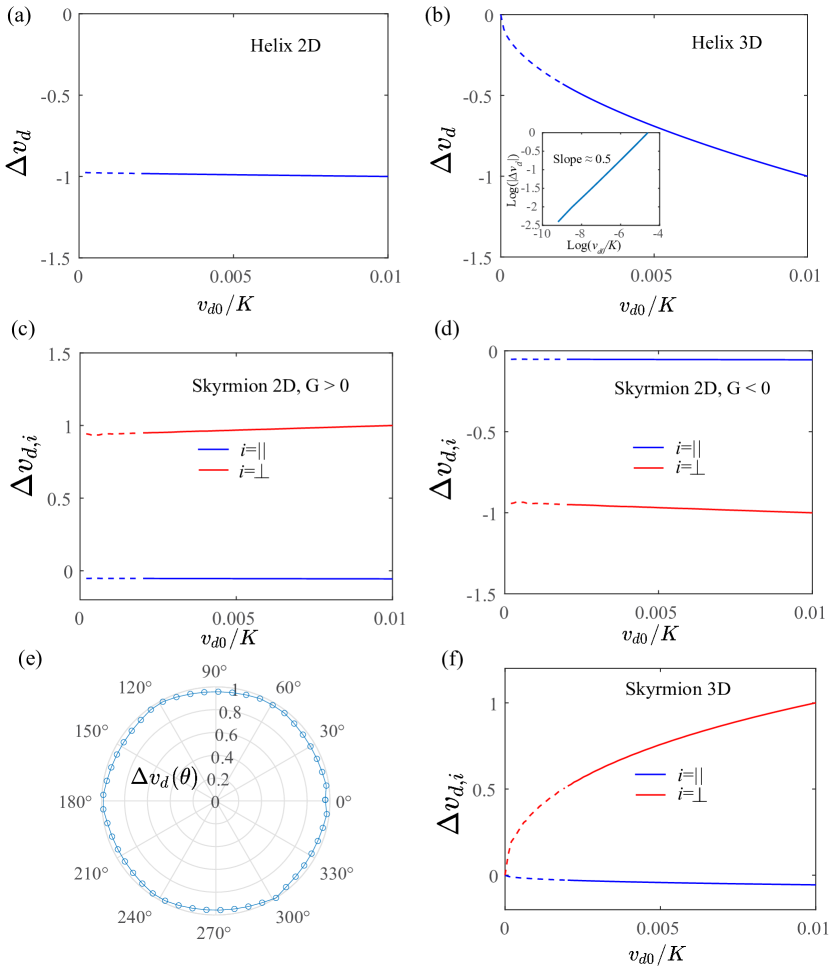
Figure 2: (a) and (b) The correction $\Delta v_{d}$ versus $v_{d0}$ (in units of $K$) for the 2D and 3D HL state, respectively. (c) and (d) The correction $\Delta\bm{v}_{d}$ versus $v_{d0}$ (in units of $K$) for the 2D SkX with $G=4\pi$ and $G=-4\pi$, respectively, where the longitudinal (transverse) component is in blue (red). The 3D SkX case is plotted in (f) with $G=4\pi$. (e) The angular-dependence of $|\Delta\bm{v}_{d}(\theta)|$, where $\theta$ is the angle of $\bm{v}_{d0}$. All the of $\Delta v_{d}$ in these plots has been normalized. The parameters $D=5.577\pi$, $\alpha=0.04$.

Helix case.— It is straightforward to generalize the above treatment to the helical spin order. The Thiele equation is reduced to one dimension:

$$D(\beta v_{s}-\alpha v_{d})+F=0.$$ (8)

The essential difference here is the absence of gyrotropic coupling ($G=0$). Following the same procedure [SM Sec. II], the self-consistent equation for the drift velocity is given by

$$v_{d}=v_{d0}+\int\frac{d^{d}\bm{q}}{(2\pi)^{d}}\sum_{\bm{g}}\frac{|\rho(\bm{g})|^{2}}{\alpha^{2}D^{2}}\Lambda(\bm{q})q_{x}^{3}\text{Im}[\mathcal{G}(\bm{q}-\bm{g},-q_{x}v_{d})].$$ (9)

Here, $v_{d0}=\frac{\beta}{\alpha}v_{s}$, the flow direction of the HL is defined as $x$-direction. After adopting the approximation in the previous section, the analytical expression of the correction $\Delta v_{d}$ of the helical magnetic state is

$$\Delta v_{d}\approx-\chi_{d}^{HL}(v_{d0})^{\frac{d-2}{2}}$$ (10)

where $\chi_{d}^{HL}=\frac{(K_{x}K_{y})^{-1/2}|\rho_{1}|^{2}\Lambda_{0}g_{0}^{3}}{4\alpha D},\text{for }d=2$ $\frac{(K_{x}K_{y}K_{z})^{-1/2}|\rho_{1}|^{2}\Lambda_{0}g_{0}^{7/2}}{2\sqrt{2}\pi(\alpha D)^{1/2}},\text{for }d=3$ with $g_{0}=\frac{\pi}{a}$. Despite different magnetic state nature, the $\Delta v_{d}$ as a function $v_{d0}$ in Eq. (10) for the HL displays a consistent scaling behavior as the one of SkX shown in Eq. (7).

Numerical evaluation.— To further justify our analytical results, we calculate the $\Delta v_{d}$ numerically according to Eqs. (6) and (9). For simplicity, we set the elastic coefficient $K_{j}$ as isotropic with $K\equiv K_{j}$. Figs. 2(a) and (b) display the correction $\Delta v_{d}$ as a function of $v_{d0}$ of HL. Note that the zero drify velocity limit should be ignored since the impurity pinning effect would be dominant in practice. When the $v_{d}$ is beyond this limit so that the pinning effect can be treated as a perturbation, which is true for the flow region, the plots clearly indicate $\Delta v_{d}\propto(v_{d0})^{\frac{d-2}{2}}$. The square root behavior in 3D ($d=3$) is explicitly checked with the log-log plot (inset of Fig. 2(b)).

Figs. 2(c) and (d) show the longitudinal component (blue) and transverse component (red) of the correction for the SkX case with positive $G$ and negative $G$, respectively. It is consistent with Eq. (7) that the transverse component is odd with respect to $G$ and is much larger than the longitudinal component as $G/\alpha D\gg 1$. This gyrotropic type correction is inherited from the Magnus forces in the Thiele equation, and this correction also implies that there exists a net change on the skyrmion Hall angle due to the impurities. Moreover, the angular dependence of the total correction $|\Delta\bm{v}_{d}|$ is shown in Figs. 2(e), where the anisotropy is very small. The $\Delta v_{d}$ as a function $v_{d0}$ also displays distinct scaling behavior between 2D [Figs. 2(c),(d)] and 3D case [Fig. 2(f)].

Overall, the scaling behavior of skyrmion similar to that of the HL in Fig. 2, as expected from our theoretical analysis. Moreover, the intrinsic drift velocity $v_{d0}$ is linearly proportional to the current density $j_{s}$ for both SkX and HL ($v_{d0}\propto j_{s}$) at large $j_{s}$. As a result, we can replace $v_{d0}$ with $j_{s}$ in the scaling relation, i.e., $\Delta v_{d}\propto(j_{s})^{\frac{d-2}{2}}$. It is worth noting that the charge density wave also respects this scaling relation [17], despite its distinct microscopic nature.

Physical interpretation.—Now we provide a physical interpretation of the observed scaling behavior: $\Delta v_{d}\propto(v_{d0})^{\frac{d-2}{2}}$. As we mentioned earlier, the dominant contribution to the drift velocity correction arises from the excitation of elastic modes. Hence, we expect the correction to be proportional to the number of excited elastic modes at a fixed $v_{d0}$. For the SkX case, these modes follow the dispersion: $v_{d0}|\bm{g}_{j}|=\mathcal{D}(\bm{k})/\sqrt{G^{2}+\alpha^{2}D^{2}}$, which can be rewritten as $v_{d0}=\bm{k}^{d}/2m^{\prime}$ with $m^{\prime}=2\pi\sqrt{G^{2}+\alpha^{2}D^{2}}/(\sqrt{3}aK)$. Next, the problem is mapped to evaluate the density of states of free fermions with an energy $v_{d0}$. Recall that the density of states of free fermion $N(E)\propto E^{\frac{d-2}{2}}$ at energy $E$. Hence, it is expected that the correction follows the same scaling: $\Delta v_{d}\propto(v_{d0})^{\frac{d-2}{2}}$ according to this argument. We emphasize that the microscopic nature of the density waves in this argument are not essential, which mainly stems from the long-wave characteristic of elastic modes. This explains why the HL and charge density wave also follow the same scaling behavior.

Micromagnetic simulation.— We now further validate our theory through solving the Landau–Lifshitz–Gilbert (LLG) equation with the spin transfer torque effect [35, 36, 37, 38, 39] (for details see SM).

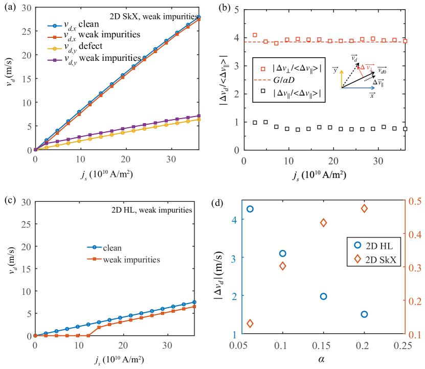
Figure 3: Simulation results of LLG equation. (a) and (c) The drift velocity $v_{d}$ versus current density $j_{s}$ (in units of $10^{10}$ A/m²) of the 2D SkX and HL at the clean and impurity case. (b) The magnitdue of longitutinal ($\Delta_{d,\parallel}$) and transverse ($\Delta_{d,\perp}$) drift velocity correction versus the current density (normalized the avegare value of $\Delta_{d,\parallel}$), where the $G/\alpha D$ ratio is highlighted (red dashed line). The coordinate relation between different vectors are shown in the inset. (d) the drift velocity correction as a function of the damping parameter $\alpha$ at $j_{s}=2\times 10^{11}\text{ A/m}^{2}$ (only $v_{d,x}$ is used for the SkX). For (a) to (c), $\alpha=0.2$ and $\beta=0.5\alpha$ are employed in the simulations.

The calculated drift velocity $v_{d}$ versus current density $j_{s}$ curves are shown in Fig. 3 for both the SkX and HL. For simplicity, we mainly focus on 2D SkX and HL with weak impurities here, where our analytical expressions from perturbation theory are applicable.

Figs. 3(a) and (c) show $v_{d}$ in the clean and disordered case with $\alpha=0.2$. The correction between these two cases at both SkX and HL is indeed insensitive to the current density within the flow limit. It is noteworthy that due to the gyrodynamcs, the SkX exhibits a much smaller depinning critical current density. Fig. 3(b) is to show that the correction along the transverse direction is obviously larger than the longitudinal one with the ratio $\sim G/\alpha D$, being consistent with Eq. (7). Interestingly, the longitudinal correction versus the damping parameter $\alpha$ of 2D SkX and HL show a positive and negative correlation, respectively [Fig. 3(d)], which is also consistent with our analytical expressions [see $\chi^{SkX}_{d}$ and $\chi^{HL}_{d}$ in Eqs. (7) and (10)]. It can also be seen that the impurity correction along longitudinal direction is typically much stronger in HL than in SkX as $\chi^{SkX}_{d}/\chi^{HL}_{d}\sim\alpha^{2}$. These distinct features between SkX and HL highlight the importance of the nontrivial topology in the sliding dynamics of density waves.

Discussion.— We have provided a thorough analysis of the sliding dynamics exhibited by the SkX and HL phases, highlighting both their similarities and differences in terms of density waves sliding with distinct topologies. Our theory could have broader applications. For instance, one can explore the relationship between the topological Hall effect and the current density in the flow region. In the clean limit, the universal linear current-velocity relation $v_{d0}\propto j_{s}$ implies that the topological Hall resistivity $\rho_{xy}$, proportional to $|(\bm{v}_{s}-\bm{v}_{d0})\times\bm{B}^{e}|/|\bm{v}_{s}|$ [15], is expected to exhibit a plateau in the flow region, as illustrated in Fig. 1(c). In the presence of impurities, the topological Hall resistivity is modified to $\rho_{xy}\propto|(\bm{v}_{s}-\bm{v}_{d0}-\Delta\bm{v}_{d})\times\bm{B}^{e}|/|\bm{v}_{s}|$. Considering that $\Delta v_{d}\propto(v_{d0})^{(d-2)/2}$, we anticipate a modified relation $\rho_{xy}=a+bj_{s}^{-2+d/2}$, where $a$ and $b$ remain independent of the current magnitude $j_{s}$. The second term, $bj_{s}^{-2+d/2}$, represents the correction from impurities. Consequently, we expect that the $\rho_{xy}$-$j_{s}$ plateau in the flow region will gradually diminish with increasing disorder.

Our theory can also be applied to investigate the sliding dynamics of a 2D Wigner crystal under out-of-plane magnetic fields [29, 30, 31]. The crucial distinction lies in the fact that the Lorentz force is typically much smaller than the damping force, whereas in the SkX, the Magnus force dominates over the damping force. In essence, the SkX represents an extreme limit of gyrodynamics.

Acknowledgment.— We thank Max Birch and Yoshinori Tokura for presenting us their Hall measurement data on the SkX, which motivated this study. N.N. was supported by JSTCREST Grants No.JMPJCR1874. Y.M.X. and Y.L. acknowledge financial support from the RIKEN Special Postdoctoral Researcher(SPDR) Program.

I The sliding dynamics of Skyrmion Crystal with pining and deformation effects

I.1 The skyrmion dynamics and Thiele equation

From the Landau-Lifshitz-Gilbert equation, it was obtained that the current-driven skyrmion dynamics are captured by the Thiele equation:

$$\bm{G}\times(\bm{v}_{s}-\bm{v}_{d})+\bm{D}(\beta\bm{v}_{s}-\alpha\bm{v}_{d})+\bm{F}=0.$$ (S1)

One can rewrite the equation as

$$-G(v_{sy}-v_{dy})+D(\beta v_{sx}-\alpha v_{dx})+F_{x}=0,$$ (S2)

$$G(v_{sx}-v_{dx})+D(\beta v_{sy}-\alpha v_{dy})+F_{y}=0.$$ (S3)

In the matrix form:

$$\begin{pmatrix}G&\alpha D\\ \alpha D&-G\end{pmatrix}\begin{pmatrix}v_{dx}\\ v_{dy}\end{pmatrix}=\begin{pmatrix}G&\beta D\\ \beta D&-G\end{pmatrix}\begin{pmatrix}v_{sx}\\ v_{sy}\end{pmatrix}+\begin{pmatrix}F_{y}\\ F_{x}\end{pmatrix}.$$ (S4)

Then,

$$\begin{pmatrix}v_{dx}\\ v_{dy}\end{pmatrix}=\begin{pmatrix}G&\alpha D\\ \alpha D&-G\end{pmatrix}^{-1}\begin{pmatrix}G&\beta D\\ \beta D&-G\end{pmatrix}\begin{pmatrix}v_{sx}\\ v_{sy}\end{pmatrix}+\begin{pmatrix}G&\alpha D\\ \alpha D&-G\end{pmatrix}^{-1}\begin{pmatrix}F_{y}\\ F_{x}\end{pmatrix}.$$ (S5)

$$\begin{pmatrix}v_{dx}\\ v_{dy}\end{pmatrix} =\frac{1}{G^{2}+\alpha^{2}D^{2}}\left[\begin{pmatrix}G^{2}+\alpha\beta D^{2}&GD(\beta-\alpha)\\ GD(\alpha-\beta)&G^{2}+\alpha\beta D^{2}\end{pmatrix}\begin{pmatrix}v_{sx}\\ v_{sy}\end{pmatrix}+\begin{pmatrix}G&\alpha D\\ \alpha D&-G\end{pmatrix}\begin{pmatrix}0&1\\ 1&0\end{pmatrix}\begin{pmatrix}F_{x}\\ F_{y}\end{pmatrix}\right],$$ (S6)

$$=\frac{1}{G^{2}+\alpha^{2}D^{2}}\left[\begin{pmatrix}G^{2}+\alpha\beta D^{2}&GD(\beta-\alpha)\\ GD(\alpha-\beta)&G^{2}+\alpha\beta D^{2}\end{pmatrix}\begin{pmatrix}v_{sx}\\ v_{sy}\end{pmatrix}+\begin{pmatrix}\alpha D&G\\ -G&\alpha D\end{pmatrix}\begin{pmatrix}F_{x}\\ F_{y}\end{pmatrix}\right]$$

Without loss of generality, we can choose the current direction to be $x$-direction: $\bm{v_{s}}=(v_{s},0)$. When the pinning force is set to be $F=0$, one can solve

$$\bm{v_{d\parallel,0}}=\frac{G^{2}+\alpha\beta D^{2}}{G^{2}+\alpha^{2}D^{2}}\bm{v_{s}},\bm{v_{d\perp,0}}=\frac{(\alpha-\beta)GD}{G^{2}+\alpha^{2}D^{2}}\hat{z}\times\bm{v_{s}}.$$ (S7)

Therefore, the longitudinal drift velocity $v_{dx}$ is proportional to the electric current when the force $\bm{F}$ is neglectable. In a general direction, we can write the intrinsic drift velocity as

$$\bm{v}_{d0} =\frac{1}{G^{2}+\alpha^{2}D^{2}}\begin{pmatrix}G^{2}+\alpha\beta D^{2}&GD(\beta-\alpha)\\ GD(\alpha-\beta)&G^{2}+\alpha\beta D^{2}\end{pmatrix}\begin{pmatrix}v_{sx}\\ v_{sy}\end{pmatrix}$$ (S10)

$$=\sqrt{\frac{1+\beta^{2}\gamma^{2}}{1+\alpha^{2}\gamma^{2}}}\begin{pmatrix}\cos\theta_{SkH}&-\sin\theta_{SkH}\\ \sin\theta_{SkH}&\cos\theta_{SkH}\end{pmatrix}\begin{pmatrix}v_{s}\cos\theta_{s}\\ v_{s}\sin\theta_{s}\end{pmatrix}$$

$$=v_{d0}\begin{pmatrix}\cos(\theta_{s}+\theta_{SkH})\\ \sin(\theta_{s}+\theta_{SkH})\end{pmatrix}.$$

Here, the angle $\theta_{s}$ is to characterize the applied current direction, the skyrmion Hall angle $\theta_{SkH}=\text{atan}\frac{\gamma(\alpha-\beta)}{1+\alpha\beta\gamma^{2}}$ with $\gamma=\frac{D}{G}$, and the magnitude of drift velocity $v_{d0}=|\bm{v}_{d0}|=v_{s}\sqrt{\frac{1+\beta^{2}\gamma^{2}}{1+\alpha^{2}\gamma^{2}}}$.

Now we show that the Thiele equation respects rotational symmetry with the principal axis along $z$-direction from Eq. (S6). The rotational operator is defined as $R_{z}=\begin{pmatrix}\cos\phi&-\sin(\phi)\\ \sin(\phi)&\cos(\phi)\end{pmatrix}$ with $\phi$ as the rotational angle. Under this rotational operation, Eq. (S6) becomes

$$R_{z}\begin{pmatrix}v_{dx}\\ v_{dy}\end{pmatrix} =\frac{1}{G^{2}+\alpha^{2}D^{2}}\left[\begin{pmatrix}G^{2}+\alpha\beta D^{2}&GD(\beta-\alpha)\\ GD(\alpha-\beta)&G^{2}+\alpha\beta D^{2}\end{pmatrix}\begin{pmatrix}v_{sx}\\ v_{sy}\end{pmatrix}+\begin{pmatrix}G&\alpha D\\ \alpha D&-G\end{pmatrix}\begin{pmatrix}0&1\\ 1&0\end{pmatrix}\begin{pmatrix}F_{x}\\ F_{y}\end{pmatrix}\right],$$ (S11)

$$=\frac{1}{G^{2}+\alpha^{2}D^{2}}\left[R_{z}\begin{pmatrix}G^{2}+\alpha\beta D^{2}&GD(\beta-\alpha)\\ GD(\alpha-\beta)&G^{2}+\alpha\beta D^{2}\end{pmatrix}R_{z}^{-1}R_{z}\begin{pmatrix}v_{sx}\\ v_{sy}\end{pmatrix}+R_{z}\begin{pmatrix}\alpha D&G\\ -G&\alpha D\end{pmatrix}R_{z}^{-1}R_{z}\begin{pmatrix}F_{x}\\ F_{y}\end{pmatrix}\right]$$

It is easy to show

$$R_{z}\begin{pmatrix}A&B\\ -B&A\end{pmatrix}R_{z}^{-1}=\begin{pmatrix}A&B\\ -B&A\end{pmatrix}$$ (S12)

with $A$ and $B$ as constant. The Eq. (S13) is simplified as

$$R_{z}\begin{pmatrix}v_{dx}\\ v_{dy}\end{pmatrix} =\frac{1}{G^{2}+\alpha^{2}D^{2}}\left[\begin{pmatrix}G^{2}+\alpha\beta D^{2}&GD(\beta-\alpha)\\ GD(\alpha-\beta)&G^{2}+\alpha\beta D^{2}\end{pmatrix}\begin{pmatrix}v_{sx}\\ v_{sy}\end{pmatrix}+\begin{pmatrix}G&\alpha D\\ \alpha D&-G\end{pmatrix}\begin{pmatrix}0&1\\ 1&0\end{pmatrix}\begin{pmatrix}F_{x}\\ F_{y}\end{pmatrix}\right],$$ (S13)

$$=\frac{1}{G^{2}+\alpha^{2}D^{2}}\left[\begin{pmatrix}G^{2}+\alpha\beta D^{2}&GD(\beta-\alpha)\\ GD(\alpha-\beta)&G^{2}+\alpha\beta D^{2}\end{pmatrix}R_{z}\begin{pmatrix}v_{sx}\\ v_{sy}\end{pmatrix}+\begin{pmatrix}\alpha D&G\\ -G&\alpha D\end{pmatrix}R_{z}\begin{pmatrix}F_{x}\\ F_{y}\end{pmatrix}\right]$$

Hence, we have shown that the Thiele equation respects out-of-plane rotational symmetry.

I.2 The correction on the drifted velocity due to the pining and deformation effects

Let us define the displacement of skyrmion lattice as $\bm{u}(\bm{r},t)$ so that the drift velocity $\bm{v_{d}}(\bm{r},t)=\frac{\partial\bm{u}(\bm{r},t)}{\partial t}$. The force is given by

$$\bm{F}(\bm{r},t) =\bm{F}_{imp}+\bm{F}_{de}$$ (S14)

$$\bm{F}_{imp} =-\sum_{i}\nabla U(\bm{r}+\bm{u}(\bm{r},t)-\bm{r}_{i})\rho(\bm{r})=\bm{f}_{imp}(\bm{r}+\bm{u}(\bm{r},t))\rho(\bm{r})$$ (S15)

$$\bm{F}_{de} =\int d\bm{r^{\prime}}\mathcal{D}(\bm{r}-\bm{r^{\prime}})\bm{u}(\bm{r^{\prime}},t^{\prime}),$$ (S16)

where $\bm{F}_{im}$ describes the pining effect from impurities and $\bm{F}_{de}$ arises from the deformation of skyrmion lattice, $U(\bm{r}-\bm{r}_{i})$ is the impurity potential around the site $\bm{r}_{i}$. $\rho(\bm{r})$ is the skyrmion densities.

$$\frac{\partial\bm{u}(\bm{r},t)}{\partial t} =\frac{1}{G^{2}+\alpha^{2}D^{2}}\left[\begin{pmatrix}G^{2}+\alpha\beta D^{2}&GD(\beta-\alpha)\\ GD(\alpha-\beta)&G^{2}+\alpha\beta D^{2}\end{pmatrix}\begin{pmatrix}v_{sx}\\ v_{sy}\end{pmatrix}+\begin{pmatrix}\alpha D&G\\ -G&\alpha D\end{pmatrix}\int d\bm{r^{\prime}}\mathcal{D}(\bm{r}-\bm{r^{\prime}})\begin{pmatrix}u_{x}(\bm{r^{\prime}},t)\\ u_{y}(\bm{r^{\prime}},t)\end{pmatrix}\right]$$ (S17)

$$+\frac{1}{G^{2}+\alpha^{2}D^{2}}\begin{pmatrix}\alpha D&G\\ -G&\alpha D\end{pmatrix}\bm{f}_{imp}(\bm{r}+\bm{u}(\bm{r},t))\rho(\bm{r}).$$

The displacement vector can be expanded around the uniform motion,

$$\bm{u}(\bm{r},t)=\bm{v_{d}}t+\tilde{\bm{u}}(\bm{r},t).$$ (S18)

Here, $\bm{v_{d}}$ is the dominant uniform skyrmion motion velocity, $\tilde{\bm{u}}(\bm{r},t)$ characterizes a small non-uniform motion. Then the equation of motion is written as

$$\left[\frac{\partial}{\partial t}-\frac{1}{G^{2}+\alpha^{2}D^{2}}\begin{pmatrix}\alpha D&G\\ -G&\alpha D\end{pmatrix}\int d\bm{r^{\prime}}\mathcal{D}(\bm{r}-\bm{r^{\prime}})\right]\begin{pmatrix}\bm{\tilde{u}}_{x}(\bm{r^{\prime}},t)\\ \bm{\tilde{u}}_{y}(\bm{r^{\prime}},t)\end{pmatrix} =\frac{1}{G^{2}+\alpha^{2}D^{2}}\begin{pmatrix}G^{2}+\alpha\beta D^{2}&GD(\beta-\alpha)\\ GD(\alpha-\beta)&G^{2}+\alpha\beta D^{2}\end{pmatrix}\begin{pmatrix}v_{sx}\\ v_{sy}\end{pmatrix}-\bm{v_{d}}$$

$$+\frac{1}{G^{2}+\alpha^{2}D^{2}}\begin{pmatrix}\alpha D&G\\ -G&\alpha D\end{pmatrix}\bm{f}_{imp}(\bm{r}+\bm{v_{d}}t+\tilde{\bm{u}}(\bm{r},t))\rho(\bm{r}).$$

Here, we have used $\mathcal{D}(\bm{q})=0$ in the long wave limit ($\bm{q}\rightarrow 0$) so that $\int d\bm{r^{\prime}}\mathcal{D}(\bm{r}-\bm{r^{\prime}})=0$.

Let us try to solve the Green’s function of the operator at the left-hand side, which is given by

$$\left[\frac{\partial}{\partial t}-\frac{1}{G^{2}+\alpha^{2}D^{2}}\begin{pmatrix}\alpha D&G\\ -G&\alpha D\end{pmatrix}\int d\bm{r^{\prime}}\mathcal{D}(\bm{r}-\bm{r^{\prime}})\right]\mathcal{G}(\bm{r}^{\prime},t)=\delta(t)\delta(\bm{r})\begin{pmatrix}1&0\\ 0&1\end{pmatrix}$$ (S20)

It is more economical to work in the momentum space with

$$\mathcal{G}(\bm{r},t)=\int\frac{d\omega}{2\pi}\int\frac{d^{d}\bm{k}}{(2\pi)^{d}}e^{-i\omega t+i\bm{k}\cdot\bm{r}}\mathcal{G}(\bm{k},\omega).$$ (S21)

Let us define $\mathcal{D}(\bm{r})=\int\frac{d^{d}q}{(2\pi)^{d}}e^{i\bm{q}\cdot\bm{r}}\mathcal{D}(\bm{q})$, and then

$$\int d\bm{r^{\prime}}\int\mathcal{D}(\bm{r}-\bm{r^{\prime}})\mathcal{G}(\bm{r^{\prime}},t) =\int d\bm{r^{\prime}}\int\frac{d^{d}\bm{q}}{(2\pi)^{d}}e^{i\bm{q}\cdot(\bm{r}-\bm{r^{\prime}})}\mathcal{D}(\bm{q})\int\frac{d^{d}\bm{k}}{(2\pi)^{d}}\int\frac{d\omega}{2\pi}\mathcal{G}(\bm{k},\omega)e^{i(\bm{k}\cdot\bm{r^{\prime}}-\omega t)}$$ (S22)

$$=\int\frac{d^{d}\bm{k}}{(2\pi)^{d}}\int\frac{d\omega}{(2\pi)}\mathcal{G}(\bm{k},\omega)\mathcal{D}(\bm{k})e^{i(\bm{k}\cdot\bm{r}-\omega t)}.$$

In the momentum space, we find

$$\mathcal{G}^{-1}(\bm{k},\omega)=-i\omega-\frac{1}{G^{2}+(D\alpha)^{2}}\begin{pmatrix}\alpha D&G\\ -G&\alpha D\end{pmatrix}\mathcal{D}(\bm{k})$$ (S23)

Therefore, Eq. (LABEL:Eq:motion2) can be rewritten as

$$\bm{\tilde{u}}(\bm{r},t) =\int d\bm{r^{\prime}}\int dt^{\prime}\mathcal{G}(\bm{r}-\bm{r^{\prime}},t-t^{\prime})\{\frac{1}{G^{2}+\alpha^{2}D^{2}}\begin{pmatrix}G^{2}+\alpha\beta D^{2}&GD(\beta-\alpha)\\ GD(\alpha-\beta)&G^{2}+\alpha\beta D^{2}\end{pmatrix}\begin{pmatrix}v_{sx}\\ v_{sy}\end{pmatrix}-\bm{v_{d}}$$ (S24)

$$+\frac{1}{G^{2}+\alpha^{2}D^{2}}\begin{pmatrix}\alpha D&G\\ -G&\alpha D\end{pmatrix}\bm{f}_{imp}(\bm{r^{\prime}}+\bm{v_{d}}t^{\prime}+\bm{\tilde{u}}(\bm{r^{\prime}},t^{\prime}))\rho(\bm{r^{\prime}})\}.$$

In the flow limit, the perturbation from the deformation and impurity can be regarded as small in comparison with the leading order term. As a result, the displacement vector can be expanded as

$$\tilde{\bm{u}}_{0}(\bm{r},t)= \int d\bm{r^{\prime}}\int dt^{\prime}\mathcal{G}(\bm{r}-\bm{r^{\prime}},t-t^{\prime})\left[\frac{1}{G^{2}+\alpha^{2}D^{2}}\begin{pmatrix}G^{2}+\alpha\beta D^{2}&GD(\beta-\alpha)\\ GD(\alpha-\beta)&G^{2}+\alpha\beta D^{2}\end{pmatrix}\begin{pmatrix}v_{sx}\\ v_{sy}\end{pmatrix}-\bm{v_{d}}\right],$$ (S25)

$$\tilde{\bm{u}}_{1}(\bm{r},t)= \frac{1}{G^{2}+\alpha^{2}D^{2}}\int d\bm{r^{\prime}}\int dt^{\prime}\mathcal{G}(\bm{r}-\bm{r^{\prime}},t-t^{\prime})\begin{pmatrix}\alpha D&G\\ -G&\alpha D\end{pmatrix}\bm{f_{imp}}(\bm{r^{\prime}}+\bm{v_{d}}t^{\prime})\rho(\bm{r^{\prime}}),$$ (S26)

$$\tilde{\bm{u}}_{2}(\bm{r},t)= \frac{1}{G^{2}+\alpha^{2}D^{2}}\int d\bm{r^{\prime}}\int dt^{\prime}\mathcal{G}(\bm{r}-\bm{r^{\prime}},t-t^{\prime})\begin{pmatrix}\alpha D&G\\ -G&\alpha D\end{pmatrix}\nabla\bm{f_{imp}}(\bm{r^{\prime}}+\bm{v_{d}}t^{\prime})\cdot\bm{\tilde{u}_{1}}(\bm{r^{\prime}},t^{\prime})\rho(\bm{r^{\prime}}).$$ (S27)

Here, $\bm{u}_{0}$, $\bm{u}_{1}$, and $\bm{u}_{2}$ are the leading, first, and second order terms, respectively. Next, let us evaluate the volume-average velocity

$$\left<\frac{\partial\tilde{\bm{u}}(\bm{r},t)}{\partial t}\right>=\left<\frac{\partial\tilde{\bm{u}}_{0}(\bm{r},t)}{\partial t}\right>+\left<\frac{\partial\tilde{\bm{u}}_{2}(\bm{r},t)}{\partial t}\right>$$ (S28)

Note the fact that under the impurity average $\overline{f_{imp}(\bm{r^{\prime}}+vt^{\prime})}=0$ has been used so that $\bm{u}_{1}(\bm{r},t)$ would not contribute directly. Since non-uniform motion must vanish over the volume average, we can obtain a self-consistent equation for the velocity $\bm{v_{d}}$. Next, let us work out the self-consistent equation for $\bm{v_{d}}$.

The leading order

$$\frac{\partial\bm{u}_{0}(\bm{r},t)}{\partial t}=\int d\bm{r^{\prime}}\int dt^{\prime}\frac{\mathcal{G}(\bm{r}-\bm{r^{\prime}},t-t^{\prime})}{\partial t}\left[\frac{1}{G^{2}+\alpha^{2}D^{2}}\begin{pmatrix}G^{2}+\alpha\beta D^{2}&GD(\beta-\alpha)\\ GD(\alpha-\beta)&G^{2}+\alpha\beta D^{2}\end{pmatrix}\begin{pmatrix}v_{sx}\\ v_{sy}\end{pmatrix}-\bm{v_{d}}\right]$$

$$=\int d\bm{r^{\prime}}\int dt^{\prime}\int\frac{d^{d}\bm{k}}{(2\pi)^{d}}\int\frac{d\omega}{2\pi}e^{i\bm{k}\cdot(\bm{r}-\bm{r^{\prime}})-i\omega(t-t^{\prime})}(-i\omega)\mathcal{G}(\bm{k},\omega)\left[\frac{1}{G^{2}+\alpha^{2}D^{2}}\begin{pmatrix}G^{2}+\alpha\beta D^{2}&GD(\beta-\alpha)\\ GD(\alpha-\beta)&G^{2}+\alpha\beta D^{2}\end{pmatrix}\begin{pmatrix}v_{sx}\\ v_{sy}\end{pmatrix}-\bm{v_{d}}\right]$$

$$=\lim_{\omega\rightarrow 0}-i\omega\mathcal{G}(\bm{k}=0,\omega)\left[\frac{1}{G^{2}+\alpha^{2}D^{2}}\begin{pmatrix}G^{2}+\alpha\beta D^{2}&GD(\beta-\alpha)\\ GD(\alpha-\beta)&G^{2}+\alpha\beta D^{2}\end{pmatrix}\begin{pmatrix}v_{sx}\\ v_{sy}\end{pmatrix}-\bm{v_{d}}\right]$$

$$=\left[\frac{1}{G^{2}+\alpha^{2}D^{2}}\begin{pmatrix}G^{2}+\alpha\beta D^{2}&GD(\beta-\alpha)\\ GD(\alpha-\beta)&G^{2}+\alpha\beta D^{2}\end{pmatrix}\begin{pmatrix}v_{sx}\\ v_{sy}\end{pmatrix}-\bm{v_{d}}\right]$$ (S29)

As mentioned the $\left<\frac{\partial\tilde{u}_{1}(\bm{r},t)}{\partial t}\right>$ would not contribute, now let us show it explicitly. Recall that

$$\tilde{\bm{u}}_{1}(\bm{r},t)=\frac{1}{G^{2}+\alpha^{2}D^{2}}\int d\bm{r^{\prime}}\int dt^{\prime}\mathcal{G}(\bm{r}-\bm{r^{\prime}},t-t^{\prime})\begin{pmatrix}\alpha D&G\\ -G&\alpha D\end{pmatrix}\bm{f_{imp}}(\bm{r^{\prime}}+\bm{v_{d}}t^{\prime})\rho(\bm{r^{\prime}})$$ (S30)

Then,

$$\frac{\partial\bm{\tilde{u}}_{1}(\bm{r},t)}{\partial t} =\int d\bm{r^{\prime}}\int dt^{\prime}\frac{1}{G^{2}+\alpha^{2}D^{2}}\mathcal{G}(\bm{r}-\bm{r^{\prime}},t-t^{\prime})\begin{pmatrix}\alpha D&G\\ -G&\alpha D\end{pmatrix}\bm{f_{imp}}(\bm{r^{\prime}}+\bm{v_{d}}t^{\prime})\rho(\bm{r^{\prime}})$$ (S34)

$$=-\frac{1}{G^{2}+\alpha^{2}D^{2}}\int d\bm{r^{\prime}}\int dt^{\prime}\int\frac{d^{d}\bm{k}}{(2\pi)^{d}}\int\frac{d\omega}{2\pi}e^{i\bm{k}\cdot(\bm{r}-\bm{r^{\prime}})-i\omega(t-t^{\prime})}\mathcal{G}(\bm{k},\omega)\begin{pmatrix}\alpha D&G\\ -G&\alpha D\end{pmatrix}\times$$

$$\int\frac{d^{d}\bm{q}}{(2\pi)^{d}}\begin{pmatrix}iq_{x}\\ iq_{y}\end{pmatrix}\overline{U_{\bm{q}}}e^{i\bm{q}\cdot(\bm{r^{\prime}}+\bm{v_{d}}t^{\prime})}\rho(\bm{r}^{\prime})$$

$$=0,$$

because after averaging over the impurity configurations, $\overline{U_{\bm{k}}}=0$.

Now let us look at the second-order term

$$\frac{\partial\bm{\tilde{u}}_{2}(\bm{r},t)}{\partial t}= \frac{1}{G^{2}+\alpha^{2}D^{2}}\int d\bm{r^{\prime}}\int dt^{\prime}\frac{\partial\mathcal{G}(\bm{r}-\bm{r^{\prime}},t-t^{\prime})}{\partial t}\begin{pmatrix}\alpha D&G\\ -G&\alpha D\end{pmatrix}\nabla\bm{f_{imp}}(\bm{r^{\prime}}+\bm{v_{d}}t^{\prime})\cdot\bm{\tilde{u}_{1}}(\bm{r^{\prime}},t^{\prime})\rho(\bm{r^{\prime}}).$$ (S35)

Note that

$$\nabla\bm{f_{imp}}(\bm{r^{\prime}}+\bm{v_{d}}t^{\prime})\cdot\bm{\tilde{u}_{1}}(\bm{r^{\prime}},t^{\prime}) =-\int\frac{d^{d}\bm{q}}{(2\pi)^{d}}U(\bm{q})e^{i\bm{q}\cdot(\bm{r^{\prime}}+\bm{v_{d}}t^{\prime})}\begin{pmatrix}q_{x}^{2}&q_{x}q_{y}\\ q_{x}q_{y}&q_{y}^{2}\end{pmatrix}\begin{pmatrix}\tilde{u}_{1x}(\bm{r^{\prime}},t^{\prime})\\ \tilde{u}_{1y}(\bm{r^{\prime}},t^{\prime})\end{pmatrix}$$ (S36)

Substitute the form of $\tilde{\bm{u}}_{1}(\bm{r^{\prime}},t)$,

$$\frac{\partial\bm{\tilde{u}}_{2}(\bm{r},t)}{\partial t}= -\frac{1}{(G^{2}+\alpha^{2}D^{2})^{2}}\int d\bm{r^{\prime}}\int dt^{\prime}\frac{\partial\mathcal{G}(\bm{r}-\bm{r^{\prime}},t-t^{\prime})}{\partial t}\begin{pmatrix}\alpha D&G\\ -G&\alpha D\end{pmatrix}\rho(\bm{r^{\prime}})\times$$ (S37)

$$\int\frac{d^{d}\bm{q}_{1}}{(2\pi)^{d}}U(\bm{q}_{1})e^{i\bm{q}_{1}(\cdot\bm{r^{\prime}}+\bm{v_{d}}t^{\prime})}\begin{pmatrix}q_{1x}^{2}&q_{1x}q_{1y}\\ q_{1x}q_{1y}&q_{1y}^{2}\end{pmatrix}\times$$

$$\int dt^{\prime\prime}\int d\bm{r^{\prime\prime}}\mathcal{G}(\bm{r}^{\prime}-\bm{r^{\prime\prime}},t^{\prime}-t^{\prime\prime})\begin{pmatrix}\alpha D&G\\ -G&\alpha D\end{pmatrix}\rho(\bm{r^{\prime\prime}})\int\frac{d^{d}\bm{q}_{2}}{(2\pi)^{d}}\begin{pmatrix}iq_{2x}\\ iq_{2y}\end{pmatrix}U(\bm{q}_{2})e^{i\bm{q}_{2}\cdot(\bm{r^{\prime\prime}}+\bm{v_{d}}t^{\prime\prime})}$$

Then write the terms at the right-hand side of the equation with their Fourier components,

$$\frac{\partial\bm{\tilde{u}}_{2}(\bm{r},t)}{\partial t} =-\frac{1}{(G^{2}+\alpha^{2}D^{2})^{2}}\int dt^{\prime}\int d\bm{r}^{\prime}\int\frac{d^{d}\bm{k}}{(2\pi)^{d}}\int\frac{d\omega}{2\pi}\mathcal{G}(\bm{k},\omega)(-i\omega)e^{i\bm{k}\cdot(\bm{r}-\bm{r^{\prime}})-i\omega(t-t^{\prime})}\begin{pmatrix}\alpha D&G\\ -G&\alpha D\end{pmatrix}\times$$ (S38)

$$\int\frac{d^{d}\bm{q}_{1}}{(2\pi)^{d}}\begin{pmatrix}q_{1x}^{2}&q_{1x}q_{1y}\\ q_{1x}q_{1y}&q_{1y}^{2}\end{pmatrix}U(\bm{q}_{1})e^{i\bm{q}_{1}\cdot(\bm{r^{\prime}}+\bm{v_{d}}t^{\prime})}\sum_{\bm{g}_{1}}\rho(\bm{g}_{1})e^{i\bm{g}_{1}\cdot\bm{r^{\prime}}}\times$$

$$\int dt^{\prime\prime}\int d\bm{r^{\prime\prime}}\int\frac{d^{d}\bm{k^{\prime}}}{(2\pi)^{d}}\int\frac{d\omega^{\prime}}{2\pi}\mathcal{G}(\bm{k^{\prime}},\omega^{\prime})e^{i\bm{k^{\prime}}\cdot(\bm{r^{\prime}}-\bm{r^{\prime\prime}})-i\omega^{\prime}(t^{\prime}-t^{\prime\prime})}\begin{pmatrix}\alpha D&G\\ -G&\alpha D\end{pmatrix}\sum_{\bm{g}_{2}}\rho(\bm{g}_{2})e^{i\bm{g}_{2}\cdot\bm{r^{\prime\prime}}}\times$$

$$\int\frac{d^{d}\bm{q}_{2}}{(2\pi)^{d}}\begin{pmatrix}iq_{2x}\\ iq_{2y}\end{pmatrix}U(\bm{q}_{2})e^{i\bm{q}_{2}\cdot(\bm{r^{\prime\prime}}+\bm{v_{d}}t^{\prime\prime})}$$

We can take integrals with respect to the space and time, and take the average over disorders, several delta functions would appear on the right-hand side:

$$\overline{U(\bm{q}_{1})U(\bm{q}_{2})} =(2\pi)^{d}\Lambda(\bm{q}_{2})\delta(\bm{q}_{1}+\bm{q}_{2}),$$ (S39)

$$\int dt^{\prime}e^{i\omega t^{\prime}}e^{i\bm{q}_{1}\cdot\bm{v_{d}}t^{\prime}}e^{-i\omega^{\prime}t^{\prime}} =2\pi\delta(\omega-\omega^{\prime}+\bm{q}_{1}\cdot\bm{v_{d}}),$$ (S40)

$$\int d\bm{r^{\prime}}e^{-i\bm{k}\cdot\bm{r^{\prime}}}e^{i\bm{q}_{1}\cdot\bm{r^{\prime}}}e^{i\bm{g}_{1}\cdot\bm{r^{\prime}}}e^{i\bm{k^{\prime}}\cdot\bm{r^{\prime}}} =(2\pi)^{d}\delta(\bm{k^{\prime}}-\bm{k}+\bm{q}_{1}+\bm{g}_{1}),$$ (S41)

$$\int dt^{\prime\prime}e^{i\omega^{\prime}t^{\prime\prime}}e^{i\bm{q}_{2}\cdot\bm{v_{d}}t^{\prime\prime}} =2\pi\delta(\omega^{\prime}+\bm{q}_{2}\cdot\bm{v_{d}}),$$ (S42)

$$\int d\bm{r^{\prime\prime}}e^{-i\bm{k^{\prime}}\cdot\bm{r^{\prime\prime}}}e^{i\bm{g}_{2}\cdot\bm{r^{\prime\prime}}}e^{i\bm{q}_{2}\cdot\bm{r^{\prime\prime}}} =(2\pi)^{d}\delta(\bm{g}_{2}+\bm{q}_{2}-\bm{k^{\prime}}).$$ (S43)

Take the volume average, and consider constraints from delta functions: $\bm{q}_{2}=-\bm{q}_{1}=\bm{q}$, $\bm{g}_{1}=-\bm{g}_{2}=\bm{g}$, $\omega^{\prime}=-\bm{q}\cdot\bm{v_{d}}$, we find

$$\left<\frac{\partial\bm{\tilde{u}}_{2}(\bm{r},t)}{\partial t}\right> =\frac{1}{(G^{2}+\alpha^{2}D^{2})^{2}}\sum_{\bm{g}}\int\frac{d^{d}\bm{q}}{(2\pi)^{d}}|\rho(\bm{g})|^{2}\Lambda(\bm{q})\begin{pmatrix}\alpha D&G\\ -G&\alpha D\end{pmatrix}\begin{pmatrix}q_{x}^{2}&q_{x}q_{y}\\ q_{x}q_{y}&q_{y}^{2}\end{pmatrix}\times$$ (S44)

$$\text{Im}\left[\mathcal{G}(\bm{q}-\bm{g},-\bm{q}\cdot\bm{v_{d}})\right]\begin{pmatrix}\alpha D&G\\ -G&\alpha D\end{pmatrix}\begin{pmatrix}q_{x}\\ q_{y}\end{pmatrix}.$$

Therefore,

$$\left<\frac{\partial\tilde{\bm{u}}(\bm{r},t)}{\partial t}\right> =\left[\frac{1}{G^{2}+\alpha^{2}D^{2}}\begin{pmatrix}G^{2}+\alpha\beta D^{2}&GD(\beta-\alpha)\\ GD(\alpha-\beta)&G^{2}+\alpha\beta D^{2}\end{pmatrix}\begin{pmatrix}v_{sx}\\ v_{sy}\end{pmatrix}-\bm{v_{d}}\right]+$$ (S45)

$$\frac{1}{(G^{2}+\alpha^{2}D^{2})^{2}}\sum_{\bm{g}}\int\frac{d^{d}\bm{q}}{(2\pi)^{d}}|\rho(\bm{g})|^{2}\Lambda(\bm{q})\begin{pmatrix}G&\alpha D\\ \alpha D&-G\end{pmatrix}\begin{pmatrix}q_{x}^{2}&q_{x}q_{y}\\ q_{x}q_{y}&q_{y}^{2}\end{pmatrix}\times$$

$$\text{Im}\left[\mathcal{G}(\bm{q}-\bm{g},-\bm{q}\cdot\bm{v_{d}})\right]\begin{pmatrix}G&\alpha D\\ \alpha D&-G\end{pmatrix}\begin{pmatrix}q_{x}\\ q_{y}\end{pmatrix}$$

Set $\left<\frac{\partial\tilde{\bm{u}}(\bm{r},t)}{\partial t}\right>=0$, the self-consistent equation for the velocity is

$$\bm{v_{d}} =\frac{1}{G^{2}+\alpha^{2}D^{2}}\begin{pmatrix}G^{2}+\alpha\beta D^{2}&GD(\beta-\alpha)\\ GD(\alpha-\beta)&G^{2}+\alpha\beta D^{2}\end{pmatrix}\begin{pmatrix}v_{sx}\\ v_{sy}\end{pmatrix}+$$ (S46)

$$\frac{1}{(G^{2}+\alpha^{2}D^{2})^{2}}\sum_{\bm{g}}\int\frac{d^{d}\bm{q}}{(2\pi)^{d}}|\rho(\bm{g})|^{2}\Lambda(\bm{q})\begin{pmatrix}\alpha D&G\\ -G&\alpha D\end{pmatrix}\begin{pmatrix}q_{x}^{2}&q_{x}q_{y}\\ q_{x}q_{y}&q_{y}^{2}\end{pmatrix}\times$$

$$\text{Im}\left[\mathcal{G}(\bm{q}-\bm{g},-\bm{q}\cdot\bm{v_{d}})\right]\begin{pmatrix}\alpha D&G\\ -G&\alpha D\end{pmatrix}\begin{pmatrix}q_{x}\\ q_{y}\end{pmatrix}.$$

As argued in the main text, the largest imaginary part is contributed by $\bm{k}=\bm{q}-\bm{g}$ in long wave limit ($\bm{k}$ is small). To further proceed, let us evaluate $\text{Im}[\mathcal{G}(\bm{k},\omega)]$.

$$\mathcal{G}(\bm{k},\omega)=\frac{1}{-i\omega-\frac{1}{G^{2}+(D\alpha)^{2}}\begin{pmatrix}\alpha D&G\\ -G&\alpha D\end{pmatrix}\mathcal{D}(\bm{k})}=-\frac{G^{2}+\alpha^{2}D^{2}}{\lambda(\bm{k})}i\omega-\frac{\mathcal{D}(\bm{k})}{\lambda(\bm{k})}\begin{pmatrix}\alpha D&-G\\ G&\alpha D\end{pmatrix},$$ (S47)

where

$$\lambda(\bm{k})=[\mathcal{D}(\bm{k})+\omega(i\alpha D+G)][\mathcal{D}(\bm{k})+\omega(i\alpha D-G)]=\mathcal{D}(\bm{k})^{2}-(G^{2}+\alpha^{2}D^{2})\omega^{2}+2i\alpha D\omega\mathcal{D}(\bm{k}).$$ (S48)

The imaginary part of Green’s function is given by

$$\text{Im}[\mathcal{G}(\bm{k},\omega)] =-\frac{(G^{2}+\alpha^{2}D^{2})[\mathcal{D}^{2}(\bm{k})-(G^{2}+\alpha^{2}D^{2})\omega^{2}]\omega}{[\mathcal{D}^{2}(\bm{k})-(G^{2}+\alpha^{2}D^{2})\omega^{2}]^{2}+4\alpha^{2}D^{2}\omega^{2}\mathcal{D}^{2}(\bm{k})}$$ (S49)

$$+\frac{2\alpha D\omega\mathcal{D}^{2}(\bm{k})}{[\mathcal{D}^{2}(\bm{k})-(G^{2}+\alpha^{2}D^{2})\omega^{2}]^{2}+4\alpha^{2}D^{2}\omega^{2}\mathcal{D}^{2}(\bm{k})}\begin{pmatrix}\alpha D&-G\\ G&\alpha D\end{pmatrix}.$$

The largest imaginary part is given by the real mode $\omega_{\bm{k}}=\mathcal{D}(\bm{k})/\sqrt{G^{2}+\alpha^{2}D^{2}}$. As a result, the first term in $\text{Im}[\mathcal{G}(\bm{k},\omega)]$ can be negligible. In 2D, we can expand

$$\mathcal{D}(\bm{k})=K_{x}k_{x}^{2}+K_{y}k_{y}^{2}.$$ (S50)

Now we can show that

$$\int\frac{d^{2}\bm{k}}{(2\pi)^{2}}\frac{2\alpha D\omega\mathcal{D}^{2}(\bm{k})}{[\mathcal{D}^{2}(\bm{k})-(G^{2}+\alpha^{2}D^{2})\omega^{2}]^{2}+4\alpha^{2}D^{2}\omega^{2}\mathcal{D}^{2}(\bm{k})}$$

$$=(K_{x}K_{y})^{-1/2}\int_{0}^{+\infty}\frac{dk^{\prime}2\pi k^{\prime}}{(2\pi)^{2}}\frac{2\alpha D\omega k^{\prime 4}}{(k^{\prime 4}-(G^{2}+\alpha^{2}D^{2})\omega^{2})^{2}+4\alpha^{2}D^{2}\omega^{2}k^{\prime 4}}$$

$$=\frac{(K_{x}K_{y})^{-1/2}\text{sgn}(\omega)}{4}.$$ (S51)

where the integral $\int_{0}^{+\infty}dt\frac{t^{2}}{(t^{2}-\frac{\sqrt{G^{2}+\alpha^{2}D^{2}}}{2\alpha D})^{2}+t^{2}}=\frac{\pi}{2}$ is used with $t=\frac{k^{\prime 2}}{2\alpha D|\omega|}$. Note that $\alpha D\neq 0$ is taken. The multiplications between matrices give

$$\begin{pmatrix}\alpha D&G\\ -G&\alpha D\end{pmatrix}\begin{pmatrix}q_{x}^{2}&q_{x}q_{y}\\ q_{x}q_{y}&q_{y}^{2}\end{pmatrix}\begin{pmatrix}\alpha D&-G\\ G&\alpha D\end{pmatrix}\begin{pmatrix}\alpha D&G\\ -G&\alpha D\end{pmatrix}\begin{pmatrix}q_{x}\\ q_{y}\end{pmatrix} =(G^{2}+\alpha^{2}D^{2})(q_{x}^{2}+q_{y}^{2})\begin{pmatrix}Gq_{y}+\alpha Dq_{x}\\ -Gq_{x}+\alpha Dq_{y}\end{pmatrix}.$$ (S52)

Finally, we obtain

$$\delta v_{d}=\frac{(K_{x}K_{y})^{-1/2}}{4(G^{2}+\alpha^{2}D^{2})}\sum_{\bm{g}}|\rho(\bm{g})|^{2}\Lambda(\bm{g})\text{sgn}(-\bm{g}\cdot\bm{v}_{d0})|\bm{g}|^{2}\begin{pmatrix}Gg_{y}+\alpha Dg_{x}\\ -Gg_{x}+\alpha Dg_{y}\end{pmatrix}$$ (S53)

We have shown that $\delta v_{d}$ respects out-of-plane rotational symmetry in the main text, which is inherited from the Theiele equation. Without loss of generality, let us set $v_{d0}$ to be along $x$-direction. In this case, after summing over the six smallest $\bm{g}$ vectors: $\bm{g}_{j}=\sqrt{3}\kappa_{0}(\sin\frac{(j-1)\pi}{3},\cos\frac{(j-1)\pi}{3})$ with $\kappa_{0}=\frac{4\pi}{3a}$, $j$ are integers from 1 to 6, we find

$$\delta\bm{v}_{d}=\frac{9\kappa_{0}^{3}|\rho_{1}|^{2}\Lambda_{0}\alpha D}{4\sqrt{K_{x}K_{y}}(G^{2}+\alpha^{2}D^{2})}\begin{pmatrix}-1\\ \frac{G}{\alpha D}\end{pmatrix}$$ (S54)

where $\rho_{1}=\rho(g_{j}),\Lambda_{0}=\Lambda(g_{j})$. In the 3D case,

$$\mathcal{D}(\bm{k})=K_{x}k_{x}^{2}+K_{y}k_{y}^{2}+K_{z}k_{z}^{2}.$$ (S55)

Then,

$$\int\frac{d^{3}\bm{k}}{(2\pi)^{3}}\frac{2\alpha D\omega\mathcal{D}^{2}(\bm{k})}{[\mathcal{D}^{2}(\bm{k})-(G^{2}+\alpha^{2}D^{2})\omega^{2}]^{2}+4\alpha^{2}D^{2}\omega^{2}\mathcal{D}^{2}(\bm{k})}$$

$$=(K_{x}K_{y}K_{z})^{-1/2}\int_{0}^{+\infty}\frac{4\pi k^{\prime 2}dk^{\prime}}{(2\pi)^{3}}\frac{2\alpha D\omega k^{\prime 4}}{(k^{\prime 4}-(G^{2}+\alpha^{2}D^{2})\omega^{2})^{2}+4\alpha^{2}D^{2}\omega^{2}k^{\prime 4}}$$

$$=\frac{(K_{x}K_{y}K_{z})^{-1/2}\Gamma(\frac{G^{2}+\alpha^{2}D^{2}}{4\alpha^{2}D^{2}})\text{sgn}(\omega)\sqrt{2\alpha D|\omega|}}{2\pi^{2}}.$$ (S56)

where $\Gamma(a)=\int_{0}^{+\infty}dx\frac{x^{6}}{(x^{4}-a)^{2}+x^{4}}$. Similarly, we can obtain

$$\delta v_{d}=\frac{(2\alpha D)^{1/2}(K_{x}K_{y}K_{z})^{-1/2}\Gamma(\frac{G^{2}+\alpha^{2}D^{2}}{4\alpha^{2}D^{2}})}{2\pi^{2}(G^{2}+\alpha^{2}D^{2})}\sum_{\bm{g}}|\rho(\bm{g})|^{2}\Lambda(\bm{g})\text{sgn}(-\bm{g}\cdot\bm{v}_{d0})\sqrt{|\bm{g}\cdot\bm{v}_{d0}|}|\bm{g}|^{2}\begin{pmatrix}Gg_{y}+\alpha Dg_{x}\\ -Gg_{x}+\alpha Dg_{y}\end{pmatrix}.$$ (S57)

After summing over the six smallest $\bm{g}$ vectors, we find

$$\delta\bm{v}_{d}=\frac{9\sqrt{3}\kappa_{0}^{7/2}\Gamma(\frac{G^{2}+\alpha^{2}D^{2}}{4\alpha^{2}D^{2}})|\rho_{1}|^{2}\Lambda_{0}\alpha D\sqrt{\alpha Dv_{d0}}}{\pi^{2}\sqrt{K_{x}K_{y}K_{z}}(G^{2}+\alpha^{2}D^{2})}\begin{pmatrix}-1\\ \frac{G}{\alpha D}\end{pmatrix}.$$ (S58)

II Helical spin order case

In this section, we consider the helical spin order case. Without loss of generality, we denote the helical spin order has a variation along $x$-direction. The Thiele equation for the helical spin order would be

$$D(\beta v_{s}-\alpha v_{d})+F=0.$$ (S59)

For simplicity, we have omitted the index $x$ in the following. The equation of motion becomes

$$\frac{\partial u(\bm{r},t)}{\partial t}=\frac{\beta}{\alpha}v_{s}+\frac{1}{\alpha D}\int d\bm{r^{\prime}}\mathcal{D}(\bm{r}-\bm{r^{\prime}})u(\bm{r^{\prime}},t^{\prime})+\frac{1}{\alpha D}f_{imp}(\bm{r}+u(\bm{r},t))\rho(\bm{r}).$$ (S60)

Similarly, by defining $u(\bm{r},r)=v_{d}t+\tilde{u}(\bm{r},t)$, the equation of motion can be rewritten as

$$[\frac{\partial}{\partial t}-\frac{1}{\alpha D}\int d\bm{r^{\prime}}\mathcal{D}(\bm{r}-\bm{r^{\prime}})]\tilde{u}(\bm{r^{\prime}},t)=\frac{\beta}{\alpha}v_{s}+\frac{1}{\alpha D}f_{imp}(\bm{r}+u(\bm{r},t))\rho(\bm{r}).$$ (S61)

Let us define the Green’s function $\mathcal{G}(\bm{r},t)$ so that

$$[\frac{\partial}{\partial t}-\frac{1}{\alpha D}\int d\bm{r^{\prime}}\mathcal{D}(\bm{r}-\bm{r^{\prime}})]\tilde{u}(\bm{r^{\prime}},t)\mathcal{G}(\bm{r^{\prime}},t)=\delta(\bm{r})\delta(t).$$ (S62)

It is easy to obtain

$$\mathcal{G}^{-1}(\bm{k},\omega)=-i\omega-\frac{\mathcal{D}(\bm{k})}{\alpha D}.$$ (S63)

The displacement $\tilde{u}(\bm{r},t)$ is given by

$$\tilde{u}(\bm{r},t)=\int d\bm{r^{\prime}}\int dt^{\prime}\mathcal{G}(\bm{r}-\bm{r^{\prime}},t-t^{\prime})[\frac{\beta}{\alpha}v_{s}-v_{d}+\frac{1}{\alpha D}f_{imp}(\bm{r^{\prime}}+u(\bm{r^{\prime}},t^{\prime}))\rho(\bm{r^{\prime}})].$$ (S64)

Then up to the second order,

$$\tilde{u}_{0}(\bm{r},t) =\int d\bm{r^{\prime}}dt^{\prime}\mathcal{G}(\bm{r}-\bm{r^{\prime}},t-t^{\prime})[\frac{\beta}{\alpha}v_{s}-v_{d}],$$ (S65)

$$\tilde{u}_{1}(\bm{r},t) =\frac{1}{\alpha D}\int d\bm{r^{\prime}}\int dt^{\prime}\mathcal{G}(\bm{r}-\bm{r^{\prime}},t-t^{\prime})f_{imp}(\bm{r^{\prime}}+v_{d}t^{\prime})\rho(\bm{r^{\prime}}),$$ (S66)

$$\tilde{u}_{2}(\bm{r},t) =\frac{1}{\alpha D}\int d\bm{r^{\prime}}\int dt^{\prime}\mathcal{G}(\bm{r}-\bm{r^{\prime}},t-t^{\prime})\partial_{x}f_{imp}(\bm{r^{\prime}}+v_{d}t^{\prime})\tilde{u}_{1}(\bm{r^{\prime}},t^{\prime})\rho(\bm{r^{\prime}}).$$ (S67)

Following a similar procedure in Sec. II, using $\braket{\frac{\partial u(\bm{r},t)}{\partial t}}=0$, we obtain

$$v_{d}=v_{d0}+\frac{1}{\alpha^{2}D^{2}}\sum_{\bm{g}}|\rho(\bm{g})|^{2}\int\frac{d^{d}\bm{q}}{(2\pi)^{d}}\Lambda(\bm{q})q_{x}^{3}\text{Im}[\mathcal{G}(\bm{q}-\bm{g},-q_{x}v_{d})].$$ (S68)

where the intrinsic drift velocity $v_{d0}=\frac{\beta}{\alpha}v_{s}$. Consider the $\text{Im}[G(\bm{k},\omega)]$ is dominant in the long wave limit ($\bm{k}\rightarrow 0$) and expand $\mathcal{D}(\bm{k})=K_{x}k_{x}^{2}+K_{y}k_{y}^{2}$ in $d=2$, we find

$$v_{d}\approx v_{d0}-\frac{(K_{x}K_{y})^{-1/2}}{8\alpha D}\sum_{\bm{g}}|\rho(\bm{g})|^{2}\Lambda(\bm{g})|g_{x}|^{3}$$ (S69)

and similarly in $d=3$ case, $\mathcal{D}(\bm{k})=K_{x}k_{x}^{2}+K_{y}k_{y}^{2}+K_{z}k_{z}^{2}$, we obtain

$$v_{d}\approx v_{d0}-\frac{(K_{x}K_{y}K_{z})^{-1/2}}{4\sqrt{2}\pi(\alpha D)^{1/2}}\sum_{\bm{g}}|\rho(\bm{g})|^{2}\Lambda(\bm{g})|g_{x}|^{3}\sqrt{|g_{x}v_{d0}|}.$$ (S70)

After summing over the smallest reciprocal lattice vectors for the helix: $\bm{g}=(\pm 1,0)g_{0}$ with $g_{0}=\frac{\pi}{a}$, the correction

$$\Delta v_{d}=\frac{\beta}{\alpha}v_{s}-\chi^{HL}_{d}(v_{d0})^{\frac{d-2}{2}}$$ (S71)

where

$$\chi_{d}^{HL}=\begin{cases}\frac{(K_{x}K_{y})^{-1/2}|\rho_{1}|^{2}\Lambda_{0}g_{0}^{3}}{4\alpha D},&\text{for }d=2\\ \frac{(K_{x}K_{y}K_{z})^{-1/2}|\rho_{1}|^{2}\Lambda_{0}g_{0}^{7/2}}{2\sqrt{2}\pi(\alpha D)^{1/2}},&\text{for }d=3\end{cases}$$ (S72)

Here, we have set $\rho(g_{0})=\rho_{1}$ and $\Lambda(g_{0})=\Lambda_{0}$ in this case.

III Numerical method details

III.1 Details for the main text Fig.2

The main text Fig.2 is obtained from the main text Eq. (6) and (9) by numerically integrating $\bm{q}$ and summing over the smallest reciprocal lattice $\bm{g}$ vectors. For the SkX, the $4000\times 4000$ in-plane momentum grids of $\bm{q}$ are taken with a hexagonal boundary (the boundary length is $4\kappa_{0}$); while for the HL, the $1000\times 1000$ in-plane momentum grids are taken with a square boundary (the boundary length is $4g_{0}$). In the 3D case, the 1000 out-of-plane momentum points of $\bm{q}$ within $[-2g_{0},2g_{0}]$ are used for both SkX and HL in evaluating the integral. Also, we set the elastic coefficients $K_{j}=10000$, the lattice constant $a$ as a natural unit of one, the damping parameter $\alpha=0.04$, the dissipative coefficient $D=5.577\pi$, the additional parameter $G=\pm 4\pi$ for the SkX.

III.2 Micromagnetic simulations

The micromagnetic simulations were performed using MuMax3 [35]. The Landau-Lifshitz-Gilbert (LLG) equation is numerically solved

$$\dot{\bm{s}}=-|\gamma_{0}|\bm{s}\times\bm{H}_{\text{eff}}+\alpha\bm{s}\times\dot{\bm{s}}+\frac{pa^{3}}{2eS}(\bm{j}_{s}\cdot\mathbb{\nabla})\bm{s}-\frac{pa^{3}\beta}{2eM_{s}^{2}}\bm{s}\times(\bm{j}_{s}\cdot\mathbb{\nabla})\bm{s},$$ (S73)

where s is the unit vector of spin, $\gamma_{0}$ is the gyromagnetic constant, $\alpha$ is the Gilbert damping constant, $M_{s}$ is the saturation magnetization, and $\bm{H}_{\text{eff}}=-\frac{1}{\mu_{0}M_{s}}\frac{\delta\mathcal{H}}{\delta\bm{S}}$ is the effective field. The spin transfer torque effect of the current is described by the last two terms [36, 37, 38]. $\beta$ describes the non-adiabaticity of the spin transfer torque effect. The current is applied along the x-direction in the simulations.

A typical chiral magnet can be described by the following Hamiltonian density

$$\mathcal{H}=A(\nabla\bm{S})^{2}-D\bm{S}\cdot(\nabla\times\bm{S})-\mu_{0}M_{s}\bm{B}\cdot\bm{S}$$ (S74)

The corresponding parameters and their values employed in the simulations are: the saturation magnetization $M_{s}=111$ kA/m, the exchange stiffness $A=3.645$ pJ/m, and the Dzyaloshinskii-Moriya interaction strength $D=0.567\text{ mJ/m}^{2}$. An external magnetic field $\bm{B}=0.3$ T (with its direction perpendicular to the skyrmion plane) is used in the simulations to stabilize the skyrmions. The simulations for helical state are performed at zero-field. The cell size is 1 nm $\times$ 1 nm $\times$ 1 nm.

We consider magnetic impurities with uniaxial magnetic anisotropy $\mathcal{H}_{imp}=-K_{imp}S_{z}^{2}$, where the easy-axis is perpendicular to the skyrmion 2D plane. For the weak impurity case, an impurity concentration $x=0.1\%$ and impurity strength $K_{imp}=0.2A/l^{2}$ ($l$ is the cell size) were used. For the strong impurity case, an impurity concentration $x=0.5\%$ and impurity strength $K_{imp}=0.6A/l^{2}$ were used. The simulation results are averaged over 100 impurity distributions. The skyrmion velocity is extracted by using the emergent electric field method [39]. For each current density, the emergent electric field is also averaged over 100 time steps in order to get the skyrmion velocity. For the transverse correction, the damping value $\alpha=0.2$ is employed in the main text Figs. 3(a) and (b) for computational efficiency, as using smaller damping values results in significantly longer simulation times to obtain a reasonable correction along the transverse direction.

References

Supplementary Material for “ Sliding Dynamics of Current-Driven Skyrmion Crystal and Helix in Chiral Magnets ”
Ying-Ming Xie,1 Yizhou Liu,1 Nato Nagaosa,1
1 RIKEN Center for Emergent Matter Science (CEMS), Wako, Saitama 351-0198, Japan