Toward Robustness in Multi-label Classification:
A Data Augmentation Strategy against Imbalance and Noise

Abstract

Multi-label classification poses challenges due to imbalanced and noisy labels in training data. We propose a unified data augmentation method, named BalanceMix, to address these challenges. Our approach includes two samplers for imbalanced labels, generating minority-augmented instances with high diversity. It also refines multi-labels at the label-wise granularity, categorizing noisy labels as clean, re-labeled, or ambiguous for robust optimization. Extensive experiments on three benchmark datasets demonstrate that BalanceMix outperforms existing state-of-the-art methods. We release the code at https://github.com/DISL-Lab/BalanceMix.

Introduction

The issue of data-label quality emerges as a major concern in the practical use of deep learning, potentially resulting in catastrophic failures when deploying models in real-world test scenarios (Whang et al. 2021). This concern is magnified in multi-label classification, where instances can be associated with multiple labels simultaneously. In this context, AI system robustness is at risk due to diverse types of data-label issues, although the task can reflect the complex relationships present in real-world data (Bello et al. 2021).

The presence of class imbalance occurs when a few majority classes occupy most of the positive labels, and positive-negative imbalance arises due to instances typically having fewer positive labels but numerous negative labels. Such imbalanced labels can dominate the optimization process and lead to underemphasizing the gradients from minority classes or positive labels. Additionally, the presence of noisy labels stems from the costly and time-consuming nature of meticulous annotation (Song et al. 2022). Labels can be corrupted by adversaries or system failures (Zhang et al. 2020). Notably, instances have both clean and incorrect labels, therefore resulting in diverse cases of noisy labels.

Three distinct types of noisy labels arise in multi-label classification, as illustrated in Fig. 1: mislabeling, where a visible object in the image is labeled incorrectly by a human or machine annotator, such as a dog being labeled as a cat; random flipping, where labels are randomly flipped by an adversary regardless of the presence of other class objects, such as negative labels for a cat and a bowl being flipped independently to positive labels; and (partially) missing labels, where even humans cannot find all applicable class labels for each image, and it is more difficult to detect their absence than to detect their presence (Cole et al. 2021).

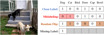
Figure 1: Examples of noisy labels in multi-label classification. $1$ and $0$ indicate positive and negative labels, symbolizing the existence of an object class.

(a) Minority Sampling (w. Noisy Multi-labels).      (b) Fine-grained Label-wise Management.             (c) Mixing Augmentation.

Figure 2: Overview of BalanceMix. Here with MS-COCO, “person” and “car” are the most frequently observed (majority) classes, whereas “hair dryer,” “scissor,” and “toaster” are the least frequently observed (minority) classes in the training data.

Ensuring the robustness of AI systems calls for a holistic approach that effectively operates within the following settings: clean, noisy, missing, and imbalanced labels at the same time. However, this task is non-trivial given that minority and noisy labels have similar behavior in learning, e.g., larger gradients, making the task even more complicated and challenging. As a result, prior studies have addressed these two problems separately in different setups, assuming either clean or well-balanced training data—i.e., imbalanced clean labels (Lin et al. 2017; Ben-Baruch et al. 2021; Du et al. 2023) and well-balanced noisy labels (Zhao and Gomes 2021; Ferreira, Costeira, and Gomes 2021; Shikun et al. 2022; Wei et al. 2023).

We address this challenge using a new data augmentation method, BalanceMix, without complex data preprocessing and architecture change. First, for imbalanced multi-labels, we maintain an additional batch sampler called a minority sampler, which samples the instances containing minority labels with high probability, as illustrated in Fig. 2(a). To counter the limited diversity in oversampling, we interpolate the instances sampled from the minority sampler with those sampled from a random sampler using the Mixup (Zhang et al. 2018) augmentation. By mixing with a higher weight to the random instances, the sparse context of the oversampled instances literally percolates through the majority of training data without losing diversity. Minority sampling in Fig. 2(a) followed by the Mixup augmentation in Fig. 2(c) is called minority-augmented mixing.

Then, for noisy multi-labels, we incorporate fine-grained label-wise management to feed high-quality multi-labels into the augmentation process. Unlike existing robust learning methods such as Co-teaching (Han et al. 2018) which consider each instance as a candidate for selection or correction, we should move to a finer granularity and consider each label as a candidate. As illustrated in Fig. 2(b), the label-wise management step categorizes the entire set of noisy labels into three subsets: clean labels which are expected to be correct with high probability; re-labeled labels whose flipping is corrected with high confidence; and ambiguous labels which need to be downgraded in optimization. Putting our solutions for imbalanced and noisy labels together, BalanceMix is completed, as illustrated in Fig. 2.

Our technical innovations are successfully incorporated into the well-established techniques of oversampling and Mixup, enabling easy integration into the existing training pipeline. Our contributions are threefold: (1) BalanceMix serves as a versatile data augmentation technique, demonstrating reliable performance across clean, noisy, missing, and imbalanced labels. (2) BalanceMix avoids overfitting to minority classes and incorrect labels thanks to minority-augmented mixing with fine-grained label management. (3) BalanceMix outperforms existing prior arts and reaches 91.7mAP on the MS-COCO data, which is the state-of-the-art performance with the ResNet backbone.

Related Work

Multi-label with Imbalance.

One of the main trends in this field is solving long-tail class imbalance and positive-negative label imbalance. There have been classical resampling approaches (Wang, Minku, and Yao 2014; Loyola-González et al. 2016) for imbalance, but they are mostly designed for a single-label setup. A common solution for class imbalance with multi-labels is the focal loss (Lin et al. 2017), which down-weights the loss value of each label gradually as a model’s prediction confidence increases, highlighting difficult-to-learn minority class labels; however, it can lead to overfitting to incorrect labels. The asymmetric focal loss (ASL) (Ben-Baruch et al. 2021) modifies the focal loss to operate differently on positive and negative labels for the imbalance. (Yuan et al. 2023) proposed a balance masking strategy using a graph-based approach.

Multi-label with (Partially) Missing Labels.

Annotation in the multi-label setup becomes harder as the number of classes increases. Subsequently, the need to handle missing labels has recently gained a lot of attention. A simple solution is regarding all the missing labels as negative labels (Wang et al. 2014), but it leads to overfitting to incorrect negative ones. There have been several studies with deep neural networks (DNNs). (Durand, Mehrasa, and Mori 2019) adopted curriculum learning for pseudo-labeling based on model predictions. (Huynh and Elhamifar 2020) used the inferred dependencies among labels and images to prevent overfitting. Recently, (Cole et al. 2021) and (Kim et al. 2022, 2023) addressed the hardest version, where only a single positive label is provided for each instance. They proposed multiple solutions including label smoothing, expected positive regularization, and label selection and correction. However, the imbalance problem is overlooked, and all the labels are simply assumed to be clean.

Classification with Noisy Labels.

For single-label classification, learning with noisy labels has established multiple directions. Most approaches are based on the memorization effect of DNNs, in which simple and generalized patterns are prone to be learned before the overfitting to noisy patterns (Arpit et al. 2017). More specifically, instances with small losses or consistent predictions are treated as clean instances, as in Co-teaching (Han et al. 2018), O2U-Net (Huang et al. 2019), and CNLCU (Xia et al. 2022); instances are re-labeled based on a model’s predictions for label correction, as in SELFIE (Song, Kim, and Lee 2019) and SEAL (Chen et al. 2021). A considerable effort has also been made to use semi-supervised learning, as in DivideMix (Li, Socher, and Hoi 2020) and PES (Bai et al. 2021). In addition, a few studies have addressed class imbalance in the noisy single-label setup (Wei et al. 2021; Ding et al. 2022), but they cannot be immediately applied to the multi-label setup owing to their inability to handle the various types of label noise caused by the nature of having both clean and incorrect labels in one instance.

For multi-label classification with noisy labels, there has yet to be studied actively owing to the inherent complexity including diverse types of label noise and imbalance. CbMLC (Zhao and Gomes 2021) addresses label noise by proposing a context-based classifier, but its architecture is confined to graph neural networks and requires large pre-trained word embeddings. A method by Hu et al.(Hu et al. 2018) utilizes a teacher-student network with feature transformation. SELF-ML (Ferreira, Costeira, and Gomes 2021) re-labels an incorrect label using a combination of clean labels, but it works only when multi-labels can be defined as attributes associated with each other. ASL (Ben-Baruch et al. 2021) solves the problem of mislabeling by shifting the prediction probability of low-confidence negative labels, making their losses close to zero in optimization. T-estimator (Shikun et al. 2022) solves the estimation problem of the noise transition matrices in the multi-label setting.

Oversampling with Mixup.

Prior studies have applied Mixup to address class imbalance (Guo and Wang 2021; Wu et al. 2020; Galdran, Carneiro, and González Ballester 2021; Park et al. 2022). Yet, they mainly focus on single-label classification, overlooking positive-negative imbalances and noisy labels. We propose the first approach that uses predictive confidence to dynamically adjust the degree of oversampling for both types of imbalance while employing label-wise management for noisy labels.

Problem Definition

A multi-label multi-class classification problem requires training data $\mathcal{D}$, a set of two random variables ($\mathbf{x}$, $\mathbf{y}$) which consists of an instance ($d$-dimensional feature) $\mathbf{x}$ $\in\mathcal{X}$ $(\subset\mathbb{R}^{d})$ and its multi-label $\mathbf{y}$ $\in\{0,1\}^{K}$, where $K$ is the number of applicable classes. However, in the presence of label noise, the noisy multi-label $\tilde{\mathbf{y}}\in\{0,1\}^{K}$ possibly contains incorrect labels originated from mislabeling, random flipping, and missing labels; that is, a noisy label $\tilde{y_{k}}\in\tilde{\mathbf{y}}$ may not be equal to the true label ${y_{k}}\in{\mathbf{y}}$. Thus, let $\tilde{\mathcal{D}}=\{(\mathbf{x}_{n},\tilde{\mathbf{y}}_{n})\}_{n=1}^{N}$ be the noisy training data of size $N$.

Label Noise Modeling.

We define three types of label noise. From the statistical point of view, (1) mislabeling is defined as class-dependent label noise, where a class object in the image is incorrectly labeled as another class object that may not be visible. The ratio of a class $c_{1}$ being mislabeled as $c_{2}$ is formulated by $\rho_{c_{1}\rightarrow c_{2}}\!\!=\!\!p(\tilde{y}_{c_{1}}\!\!=\!\!0,\tilde{y}_{c_{2}}\!\!=\!\!1|y_{c_{1}}\!\!=\!\!1,y_{c_{2}}\!\!=\!\!0)$. In contrast, (2) random flipping is class-independent label noise, where the presence (or absence) of a class $c$ is randomly flipped with a probability of $\rho_{c}=p(\tilde{y}_{c}=1|y_{c}=0)=p(\tilde{y}_{c}=0|y_{c}=1)$, which is independent of the presence of other classes. This scenario can be caused by an adversary’s attack or a system failure. Last, (3) missing labels from partial labeling can be considered as a type of label noise, where all missing labels are treated as negative ones.

Optimization.

To deal with multi-labels in optimization, the most widely-used approach is solving $K$ binary classification problems using the binary cross-entropy (BCE) loss. Given a DNN parameterized by $\Theta$, the DNN is updated via stochastic gradient descent to minimize the expected BCE loss on the mini-batch ${B}\subset\tilde{\mathcal{D}}$,

$$\begin{split}\mathcal{L}(B;\Theta)&=\frac{1}{|B|}\sum_{(\mathbf{x},\tilde{\mathbf{y}})\in B}\sum_{k=1}^{K}{\rm BCE}(f_{(\mathbf{x},\tilde{y}_{k})}),~{}{\rm where}\\ {\rm BCE}(f_{(\mathbf{x},\tilde{y}_{k})})&=-\tilde{y}_{k}\cdot{\rm log}(f_{(\mathbf{x},\tilde{y}_{k})})-(1\!-\!\tilde{y}_{k})\cdot{\rm log}(1\!-\!f_{(\mathbf{x},\tilde{y}_{k})}).\end{split}$$ (1)

Given the instance $\mathbf{x}$, $f_{(\mathbf{x},\tilde{y}_{k})}$ and $1\!-\!f_{(\mathbf{x},\tilde{y}_{k})}$ are the confidence in presence and absence, respectively, for the $k$-th class by the model $\Theta$. BalanceMix is built on top of this standard optimization pipeline for multi-label classification.

Methodology: BalanceMix

Our primary idea is to generate minority-augmented instances and their reliable multi-labels through data augmentation. We now detail the two main components, which achieve balanced and robust optimization by minority-augmented mixing and label-wise management. The pseudocode of BalanceMix is provided in Appendix A.

Minority-augmented Mixing

To relieve the class imbalance problem, prior studies either oversample the minority class labels or adjust their loss values (Tarekegn, Giacobini, and Michalak 2021). These methods are intuitive but rather intensify the overfitting problem since they rely on a few minority instances with limited diversity (Guo and Wang 2021). On the other hand, we leverage random instances to increase the diversity of minority instances by separately maintaining two samplers in Fig. 2.

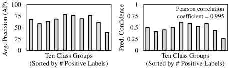
(a) Prediction Confidence.       (b) Average Precision (AP). ​​​

Figure 3: AP and Prediction confidence in COCO using the BCE loss at the 40$\%$ of training epochs, where 80 classes are partitioned into ten groups in the descending order of positive label frequency. The Pearson correlation coefficient is computed between ten class groups.

Confidence-based Minority Sampling.

Prior oversampling methods that rely on the frequency of positive labels face two key limitations. First, this frequency alone does not identify the minority multi-labels with low AP values; as illustrated in Fig. 3(a), the class group with few positive labels does not always have lower AP values due to the complexity of the two types of imbalance in the multi-label setup. Second, there is a risk of overfitting because of sticking to the same oversampling policy during the entire training period.

To address these limitations, we first propose to employ the prediction confidence $f_{(\mathbf{x},\tilde{y}_{k})}$, which exhibits a strong correlation with the AP, as shown in Fig. 3(b). We opt to oversample the instances with low prediction confidence in their multi-labels, as they are expected to contribute the most significant increase in the AP. Initially, We define two confidence scores for a specific class $k$,

$$\begin{split}{\rm P}(k)=\frac{1}{|{\mathcal{P}_{k}}|}\!\sum_{(\mathbf{x},\tilde{\mathbf{y}})\in{\mathcal{P}_{k}}}\!\!\!\!\!f_{(\mathbf{x},\tilde{y}_{k})},~{}~{}{\rm A}(k)=\frac{1}{|{\mathcal{A}_{k}}|}\!\sum_{(\mathbf{x},\tilde{\mathbf{y}})\in{\mathcal{A}_{k}}}\!\!\!\!(1\!-\!f_{(\mathbf{x},\tilde{y}_{k})}),\\ {\rm s.t.}~{}\mathcal{P}_{k}=\{(\mathbf{x},\tilde{\mathbf{y}})\in\tilde{\mathcal{D}}:\tilde{y}_{k}\!=\!1\},~{}\mathcal{A}_{k}=\{(\mathbf{x},\tilde{\mathbf{y}})\in\tilde{\mathcal{D}}:\tilde{y}_{k}\!=\!0\},\end{split}$$ (2)

which are the expected prediction confidences, respectively, for the presence (P) and absence (A) of the $k$-th class. Next, the confidence score of an instance $(\mathbf{x},\tilde{\mathbf{y}})$ is defined by aggregating Eq. (2) for all the classes,

$$\text{Score}(\mathbf{x},\tilde{\mathbf{y}})=\sum_{k=1}^{K}\mathbf{1}_{[\tilde{y}_{k}=1]}{\rm P}(k)+\mathbf{1}_{[\tilde{y}_{k}=0]}{\rm A}(k).$$ (3)

Then, the sampling probability of $(\mathbf{x},\tilde{\mathbf{y}})$ is formulated as

$$p_{\text{sampling}}\big{(}(\mathbf{x},\tilde{\mathbf{y}});\tilde{\mathcal{D}}\big{)}=\frac{1/\text{Score}(\mathbf{x},\tilde{\mathbf{y}})}{\sum_{(\mathbf{x}^{\prime},\tilde{\mathbf{y}}^{\prime})\in\tilde{\mathcal{D}}}1/{\rm Score}(\mathbf{x}^{\prime},\tilde{\mathbf{y}}^{\prime})}.$$ (4)

By doing so, we consider positive-negative imbalance together with class imbalance by relying on the prediction confidence, which marks a significant difference from existing methods (Galdran, Carneiro, and González Ballester 2021; Park et al. 2022) that considers only the class imbalance of positive labels. Further, our confidence-based sampling dynamically adjusts the degree of oversampling over a training period, mitigating the risk of overfitting. Minority instances are initially oversampled with a high probability, but the degree of oversampling gradually decreases as the imbalance problem gets resolved (see Figure 6 in Appendix B).

Mixing Augmentation.

To mix the instances from the two samplers. We adopt the Mixup (Zhang et al. 2018) augmentation because it can mix two instances even when multi-labels are assigned to them. Let $(\mathbf{x}_{R},\tilde{\mathbf{y}}_{R})$ and $(\mathbf{x}_{M},\tilde{\mathbf{y}}_{M})$ be the instances sampled from the random and minority samplers, respectively. The minority-augmented instance is generated by their interpolation,

$$\begin{gathered}\mathbf{x}^{mix}\!=\!\lambda\mathbf{x}_{R}\!+\!(1\!-\!\lambda)\mathbf{x}_{M},~{}\tilde{\mathbf{y}}^{mix}\!=\!\lambda\tilde{\mathbf{y}}_{R}\!+\!(1\!-\!\lambda)\tilde{\mathbf{y}}_{M}\!\!\\ {\rm where}~{}~{}\lambda={\rm max}(\lambda^{\prime},1-\lambda^{\prime}),\end{gathered}$$ (5)

and $\lambda^{\prime}\in[0,1]\sim{\rm Beta}(\alpha,\alpha)$. By the second row of Eq. (5), $\lambda$ becomes greater than or equal to $0.5$; thus, the instance of the random sampler amplifies diversity, while that of the minority sampler adds the context of minority classes. Mixing one random instance and one controlled (minor) instance, instead of mixing two random instances, is a simple yet effective strategy, as shown in the evaluation.

Fine-grained Label-wise Management

Before mixing the two instances by Eq. (5), to make noisy multi-labels reliable in support of robust optimization, we perform label-wise refinement.

Clean Labels.

To relieve the imbalance problem in label selection, we separately identify clean labels for each class. Let $L_{(\tilde{y}_{k}=1)}$ and $L_{(\tilde{y}_{k}=0)}$ be the sets of the BCE losses of the positive and negative labels of the $k$-th class,

$$L_{(\tilde{y}_{k}=l)}=\{{\rm BCE}(f_{(\mathbf{x},\tilde{y}_{k}=l)})~{}|~{}(\mathbf{x},\tilde{\mathbf{y}})\in\tilde{\mathcal{D}}~{}\wedge~{}\tilde{y}_{k}\in\tilde{\mathbf{y}}~{}\wedge~{}\tilde{y}_{k}=l\},\!$$ (6)

where $l$ is 1 or 0 for the positive or negative label.

Clean labels exhibit loss values smaller than noise ones due to the memorization effect of DNNs (Li, Socher, and Hoi 2020). Hence, we fit a bi-modal univariate Gaussian mixture model (GMM) to each set of the BCE losses in using the expectation-maximization (EM) algorithm, returning $2\times K$ GMM models for positive and negative labels of $K$ classes,

$$p_{\mathcal{G}}=\{(\mathcal{G}_{(\tilde{y}_{k}=1)},\mathcal{G}_{(\tilde{y}_{k}=0)})\}_{k=1}^{K}.$$ (7)

Given the BCE loss of $\mathbf{x}$ for the $k$-th positive or negative label, its clean-label probability is obtained by the posterior probability of the corresponding GMM,

$$\!p_{\mathcal{G}}(\mathbf{x},\tilde{y}_{k}=l)=\frac{\mathcal{G}_{(\tilde{y}_{k}=l)}({\rm BCE}(f_{(\mathbf{x},\tilde{y}_{k}=l)})|g)\cdot\mathcal{G}_{(\tilde{y}_{k}=l)}(g)}{\mathcal{G}_{(\tilde{y}_{k}=l)}({\rm BCE}(f_{(\mathbf{x},\tilde{y}_{k}=l)}))},\!\!\!$$ (8)

where $g$ denotes a modality for the small-loss (clean) label. Thus, a label with $p_{\mathcal{G}}>0.5$ is marked as being clean.

The time complexity of GMM modeling is $\mathcal{O}(NGD)\!=\!\mathcal{O}(N)$ and thus linear to the number of instances $N$, where the number of modalities $G\!=\!2$ and the number of dimensions $D\!=\!1$ (see (Trivedi et al. 2017) for the proof of the time complexity). Since we model the GMMs once per epoch, the cost involved is expected to be small compared with the training steps of a complex DNN.

Re-labeled Labels.

Before the overfitting to noisy labels, a model’s prediction delivers useful underlying information on correct labels (Song, Kim, and Lee 2019). Therefore, we modify the given label if it is not selected as a clean one but the model exhibits high confidence in predictions. To obtain a stable confidence from the model, we ensemble the prediction confidences on two augmented views created by RandAug (Cubuk et al. 2020). Given two differently-augmented instances from the original instance $\mathbf{x}$ whose $p_{\mathcal{G}}(\mathbf{x},\tilde{y}_{k})\leq 0.5$, the $k$-th label is re-labeled by

$$\begin{gathered}1/2\cdot(f_{({\rm aug}_{1}(\mathbf{x}),\tilde{y}_{k})}+f_{({\rm aug}_{2}(\mathbf{x}),\tilde{y}_{k})})>\epsilon~{}\Longrightarrow~{}\tilde{y}_{k}=1,\!\!\!\!\\ 1/2\cdot(f_{({\rm aug}_{1}(\mathbf{x}),\tilde{y}_{k})}+f_{({\rm aug}_{2}(\mathbf{x}),\tilde{y}_{k})})<1-\epsilon~{}\Longrightarrow~{}\tilde{y}_{k}=0,\!\!\!\!\end{gathered}$$ (9)

where $\epsilon$ is the confidence threshold for re-labeling.

Ambiguous Labels.

The untouched labels, which are neither clean nor re-labeled, are regarded as being ambiguous. These labels are potentially incorrect, but they could hold meaningful information in learning with careful treatment. To squeeze the meaningful information and reduce the potential risk, for these ambiguous labels, we execute importance reweighting which decays a loss based on the clean-label probability estimated by Eq. (8).

(a) Default.                      (b) Methods for Noisy Labels.                     (c) Methods for Missing Labels.           (d) Ours.

Figure 4: Performance ranking (1–7) from five different perspectives. BalanceMix is the most versatile to handle diverse types of label issues in multi-label classification. A number in a pentagon is its area, roughly meaning the overall performance.

Class Group		All			Many-shot			Medium-shot			Few-shot
Category	Method	0%	20%	40%	0%	20%	40%	0%	20%	40%	0%	20%	40%
Default	BCE Loss	83.4	73.1	63.8	86.9	78.4	68.4	84.5	74.0	64.3	64.3	55.5	48.0
Noisy Labels	Co-teaching	82.8	82.5	78.6	87.2	87.0	82.7	84.0	83.7	79.7	61.2	60.9	54.5
	ASL	85.0	82.8	80.3	88.4	87.4	85.4	86.3	84.0	81.8	67.5	62.5	55.6
	T-estimator	84.3	82.2	80.5	87.5	86.3	85.3	85.4	83.6	81.3	67.0	59.7	61.0
Missing Labels​​	LL-R	82.5	80.7	75.3	81.0	83.9	79.8	83.8	81.8	76.7	65.7	63.1	52.6
	LL-Ct	79.4	81.3	77.4	72.3	78.8	79.3	80.5	82.6	78.8	67.0	64.3	55.9
Proposed	BalanceMix	85.2	84.3	81.6	88.4	87.7	85.5	86.1	85.2	82.6	70.2	68.7	63.1

Table 1: Last mAPs on MS-COCO with mislabeling of $0$–$40\%$. The 1st and 2nd best values are in bold and underlined.

Optimization with BalanceMix

Given two instances sampled from the random and minority samplers, their multi-labels are first refined by the label-wise management setup. The reliability of each refined label is stored as C for clean labels, R for re-labeled labels, and U for ambiguous labels. Then, a minority-augmented instance is generated by Mixup with the mixed multi-labels. The reliability of each label of the augmented instance follows that of the instance selected by the random sampler, because it always dominates in mixing by $\lambda\geq 0.5$ in Eq. (5). The loss function of BalanceMix is defined on the minority-augmented mini-batch $B_{mix}$ by

$$\begin{gathered}\mathcal{L}_{\rm ours}(B_{mix};\Theta)=\frac{1}{|B_{mix}|}\!\!\!\!\!\!\!\!\!\sum_{~{}~{}~{}~{}~{}~{}~{}(\mathbf{x}^{mix},\tilde{\mathbf{y}}^{mix})\in B_{mix}}\!\!\!\!\!\!\!\!\!\!\!\!\!\!\!\!\ell(\mathbf{x}^{mix},\tilde{\mathbf{y}}^{mix}),\\ {\rm where}~{}~{}\ell(\mathbf{x}^{mix},\mathbf{y}^{mix})=\!\!\!\sum_{k\in{\sf C}\cup{\sf R}}\!\!\!{\rm BCE}(f_{(\mathbf{x}^{mix},\tilde{y}_{k}^{mix})})\\ +\sum_{k\in{\sf U}}p_{\mathcal{G}}(\mathbf{x}^{mix},\tilde{y}_{k}^{mix})\!\cdot\!{\rm BCE}(f_{(\mathbf{x}^{mix},\tilde{y}_{k}^{mix})}).\!\!\!\!\end{gathered}$$ (10)

We perform standard training for warm-up epochs and then apply the proposed loss function in Eq. (10).

Evaluation

Datasets.

Pascal-VOC (Everingham et al. 2010) and MS-COCO (Lin et al. 2014) are the most widely-used datasets with well-curated labels of 20 and 80 common classes. In contrast, DeepFashion (Liu et al. 2016) is a real-world in-shopping dataset with noisy weakly-annotated labels for $1,000$ descriptive attributes.

Class Group		All			Many-shot			Medium-shot			Few-shot
Category	Method	0%	20%	40%	0%	20%	40%	0%	20%	40%	0%	20%	40%
Default	BCE Loss	83.4	59.8	43.5	86.9	71.2	65.1	84.5	60.6	43.2	64.3	38.9	30.6
Noisy Labels	Co-teaching	82.8	65.5	43.6	87.2	76.1	61.9	84.0	66.8	43.8	61.2	38.3	25.9
	ASL	85.0	75.0	66.2	88.4	84.4	82.8	86.3	77.0	67.7	67.5	39.2	30.8
	T-estimator	84.3	74.3	69.9	87.5	82.6	80.8	85.4	76.0	71.5	67.4	43.6	39.1
Missing Labels​​	LL-R	82.5	74.0	69.3	81.0	77.2	76.6	83.8	75.8	71.0	65.7	46.0	38.6
	LL-Ct	79.4	73.2	70.1	72.3	75.5	76.5	80.5	75.0	71.8	67.0	45.5	41.1
Proposed	BalanceMix	85.2	76.5	74.5	88.4	84.5	81.3	86.1	78.2	76.3	70.2	46.1	43.0

Table 2: Last mAPs on MS-COCO with random flipping of $0$–$40\%$. The 1st and 2nd best values are in bold and underlined.

Datasets		MS-COCO				Pascal-VOC
Category	Method	All	Many	​​​Medium​​​	Few	All	​​​Medium​​​	Few
Default	BCE Loss	69.7	71.7	70.6	54.4	85.7	89.2	84.2
Noisy Labels	Co-teaching	68.1	61.5	69.2	59.1	80.9	87.2	78.1
	ASL	73.3	77.7	74.7	49.2	86.8	82.1	88.8
	T-estimator	16.8	43.2	16.3	3.3	86.2	88.9	85.0
Missing Labels	LL-R	74.2	75.4	75.3	58.7	89.1	91.5	88.1
	LL-Ct	76.9	77.4	78.2	57.6	89.3	91.5	88.3
Proposed	BalanceMix	77.4	76.2	78.5	61.3	92.6	94.5	91.8

Table 3: Last mAPs on MS-COCO and Pascal-VOC in the missing label (single positive label) setup.

Imbalanced and Noisy Labels.

The three datasets contain different levels of natural imbalance. Pascal-VOC, MS-COCO, and DeepFashion have the class imbalance ratios of $14$, $339$, and $239$, and the positive-negative imbalance ratios of $13$, $27$, and $3$, respectively. See the detailed analysis of the imbalance in Appendix C. We artificially contaminate Pascal-VOC and MS-COCO to add three types of label noise. First, for mislabeling, we inject class-dependent label noise. Given a noise rate $\tau$, the presence of the $i$-th class is mislabeled as that of the $j$-th class with a probability of $\rho_{i\rightarrow j}$; we follow the protocol used for a long-tail noisy label setup (Wei et al. 2021). For the two different classes $i$ and $j$,

$$\rho_{i\rightarrow j}=p(\tilde{y}_{i}=0,\tilde{y}_{j}\!=\!1|y_{i}\!=\!1)=\tau\cdot N_{j}/(N-N_{i}),$$ (11)

where $N_{i}$ is the number of positive labels for the $i$-th class. Second, for random flipping, all positive and negative labels are flipped independently with the probability of $\tau$. Third, for missing labels, we follow the single positive label setup (Kim et al. 2022), where one positive label is selected at random and the other positive labels are dropped.

Algorithms.

We use the ResNet-50 backbone pre-trained on ImageNet-1K and fine-tune using SGD with a momentum of 0.9 and resolution of $448\times 448$. We compare BalanceMix with a standard method using the BCE loss (Default) and five state-of-the-art methods, categorized into two groups. The former is to handle noisy labels based on instance-level selection, loss reweighting, and noise transition matrix estimation—Co-teaching (Han et al. 2018), ASL (Ben-Baruch et al. 2021), and T-estimator (Shikun et al. 2022). The latter is to handle missing labels based on label rejection and correction—LL-R and LL-Ct (Kim et al. 2022). For data augmentation, we apply RandAug and Mixup to all methods, except Default using only RandAug. The results of Default with Mixup are presented in Table 5.

As for our hyperparameters, the coefficient $\alpha$ for Mixup is set to be $4.0$; and the confidence threshold $\epsilon$ for re-labeling is set to be $0.975$ for the standard, mislabeling, and random flipping settings with multiple positive labels, but it is set to be $0.550$ for the missing label setting with a single positive label. More details of configuration and hyperparameter search can be found in Appendices D and E.

Evaluation Metric.

We report the overall validation (or test) mAP at the last epoch over three disjoint class subsets: many-shot (more than 10,000 positive labels), medium-shot (from 1,000 to 10,000 positive labels), and few-shot (less than 1,000 positive labels) classes. The result at the last epoch is commonly used in the literature on robustness to label noise (Han et al. 2018). We repeat every task thrice, and see Appendix F for the standard error.

Overall Analysis on Five Perspectives

Fig. 4 shows the overall performance rankings aggregated on Pascal-VOC and MS-COCO for five different perspectives: “Clean” for when label noise is not injected, “Mislabel” for when labels are mislabeled with the noise ratio of $20$–$40\%$, “Rand. Flip” for when labels are randomly flipped with the noise ratio of $20$–$40\%$, “Missing” for when the single positive label setup is used, and “Imbal.” for when few-shot classes without label noise are used.

Only BalanceMix operates in all scenarios with high performance: its minority-augmented mixing overcomes the problem of imbalanced labels while its fine-grained label-wise management adds robustness to diverse types of label noise. Except BalanceMix, the five existing methods have pros and cons. The three methods of handling noisy labels in Fig. 4(b) generally perform better for mislabeling and random flipping than the others; but the instance-level selection of Co-teaching is not robust to random flipping where a significant number of negative labels are flipped to positive ones. In contrast, the two methods of handling missing labels in Fig. 4(c) perform better with the existence of missing labels than Co-teaching, ASL, and T-estimator. LL-Ct (label correction) is more suitable than LL-R (label rejection) for mislabeling and random flipping since label correction has a potential to re-label some of incorrect labels. For the imbalance, ASL shows reasonable performance on the few-shot subset by adopting a modified focal loss.

Results on Imbalanced and Noisy Labels

We evaluate the performance of BalanceMix on MS-COCO with three types of synthetic label noise and on DeepFashion with real-world label noise. We defer the results on Pascal-VOC to Appendix F for the sake of space.

Mislabeling (Table 1).

BalanceMix achieves not only the best overall mAP (see the “All” column) with varying mislabeling ratios, but also the best mAP on few-shot classes (see the “Few-shot” column). It shows higher robustness even compared with the three methods designed for noisy labels. ASL performs well among the compared methods, but its weighting scheme of pushing higher weights to difficult-to-learn labels could lead to overfitting to difficult incorrect labels; hence, when the noise ratio increases, its performance rapidly degrades from $67.5\%$ to $55.6\%$ in the few-shot classes. Both methods for missing labels perform better than the default method (BCE), but are still vulnerable to mislabeling.

Class Group	All	Many	​​Medium​​	Few
BCE Loss	75.2	93.4	84.4	53.4
Co-teaching	66.8	90.7	81.3	32.8
ASL	76.4	94.4	85.2	55.4
T-estimator	75.4	94.7	84.8	53.1
LL-R	75.3	93.3	84.2	53.8
LL-Ct	75.2	92.6	84.2	53.8
BalanceMix	77.0	95.2	85.6	56.4

Table 4: mAPs on DeepFashion with real-world noisy multi-labels using seven multi-label classification methods.

Component​​	Clean Label	Mislabel 40%	​​Rand Flip 40%​​	Missing Label	Overall (Mean)
Default (BCE Loss)	​​​​​​​​​​​​​​​​​​83.4	​​​​​​​​​​​​​​​​​​63.3	​​​​​​​​​​​​​​​​​​43.0	​​​​​​​​​​​​​​​​​​72.6	​​​​​​​​​​​​​​​​​​65.6
$+$ Random Sampler ($\approx$ Mixup)	84.2 ($+$0.8)	67.4 ($+$3.3)	64.9 ($+$21.9)	73.3 ($+$0.7)	72.5 ($+$6.9)
$+$ Minority Sampler (in Eq. (4))	85.1 ($+$1.7)	70.2 ($+$6.9)	67.2 ($+$24.2)	74.2 ($+$1.6)	74.2 ($+$8.6)
$+$ Clean Labels (in Eq. (8))	84.9 ($-$0.2)	76.1 ($+$5.9)	74.9 ($+$7.7)	74.6 ($+$0.4)	77.6 ($+$3.4)
$+$ Re-labeled Labels (in Eq. (9))	85.3 ($+$0.4)	80.2 ($+$3.9)	74.9 ($+$0.0)	76.1 ($+$1.5)	79.1 ($+$1.5)
$+$ Ambiguous Labels (in Eq. (10))	85.3 ($+$0.0)	81.6 ($+$1.4)	74.5 ($-$0.4)	77.4 ($+$1.3)	79.7 ($+$0.6)

Table 5: Component analysis of BalanceMix on MS-COCO. The values in parentheses are the gain caused by each component.

Random Flipping (Table 2).

This is more challenging than mislabeling noise, in considering that even negative labels are flipped by a given noise ratio. Accordingly, the mAP of Co-teaching and ASL drops significantly when the noise ratio reaches $40\%$ (see the “All” column), which implies that instance selection in Co-teaching and loss reweighting in ASL are ineffective to overcome random flipping. T-estimator shows a better result at the noise ratio of $40\%$ than ASL by estimating the noise transition matrix per class. Overall, BalanceMix achieves higher robustness against a high flipping ratio of $40\%$ with fine-grained label-wise management; its performance drops by only $10.7\%p$, which is much smaller than $39.2\%p$, $18.8\%p$, and $14.4\%p$ of Co-teaching, ASL, and T-estimator, respectively. Thus, it maintains the best mAP for all class subsets in general.

Missing Labels (Table 3).

Unlike the mislabeling and random flipping, LL-R and LL-Ct generally show higher mAPs than the methods for noisy labels, because LL-R and LL-Ct are designed to reject or re-label unobserved positive labels that are erroneously considered as negative ones. Likewise, the label-wise management of BalanceMix includes the re-labeling process, fixing incorrect positive and negative labels to be correct. In addition, it shows higher mAP in the few-shot classes than LL-Ct due to the consideration of imbalanced labels. Thus, it consistently maintains its performance dominance. Meanwhile, T-estimator performs badly in MS-COCO due to the complexity of transition matrix estimation.

Real-world Noisy Labels (Table 4).

A real-world noisy dataset, DeepFashion, likely contains all the label noises—mislabeling, random flipping, and missing labels—along with class imbalance. Therefore, our motivation for a holistic approach is of importance for real use cases.

The relatively small performance gain is attributed to a small percentage (around 8%) of noise labels (Song et al. 2022) in DeepFashion, because its fine-grained labels were annotated via a crowd-sourcing platform which can be relatively reliable. The performance gain will increase for datasets with a higher noise ratio.

Component Ablation Study

We conduct a component ablation study by adding the main components one by one on top of the default method. Table 5 summarizes the mAP and average performance of each of five variants. The first variant of using only a random sampler is equivalent to the original Mixup.

First, using only a random sampler like Mixup does not sufficiently improve the model performance, but adding the minority sampler achieves sufficient improvement because it takes imbalanced labels into account. Second, exploiting only the selected clean labels increases the mAP when positive labels are corrupted with mislabeling and random flipping. However, this approach is not that beneficial in the clean and missing label setups, where all positive labels are regarded as being clean; it also simply discards all (expectedly) unclean negative labels without any treatment. Third, re-labeling complements the limitation of clean label selection, providing additional mAP gains in most scenarios. Fourth, using ambiguous labels adds further mAP improvement except for the random flipping setup.

In summary, since all the components in BalanceMix generally add a synergistic effect, leveraging all of them is recommended for use in practice. In Appendix G, we (1) analyze the impact of minority-augmented mixing on diversity changes, (2) provide the pure effect of label-wise management, and (3) report its accuracy in selecting clean labels and re-labeling incorrect labels.

Method	Backbone	Resolution	mAP (All)
MS-CMA	ResNet-101	448$\times$448	83.8
ASL	ResNet-101	448$\times$448	85.0
ML-Decoder	ResNet-101	448$\times$448	87.1
BalanceMix	ResNet-101	448$\times$448	87.4 (+0.3)
ASL	TResNet-L	448$\times$448	88.4
Q2L	TResNet-L	448$\times$448	89.2
ML-Decoder	TResNet-L	448$\times$448	90.0
BalanceMix	TResNet-L	448$\times$448	90.5 (+0.5)
ML-Decoder	TResNet-L	640$\times$640	91.1
ML-Decoder	TResNet-XL	640$\times$640	91.4
BalanceMix​​	TResNet-L	640$\times$640	91.7 (+0.6)

Table 6: State-of-the-art comparison on MS-COCO. The values in parentheses are the improvements over the latest method using the same backbone.

State-of-the-art Comparison on MS-COCO

We compare BalanceMix with several methods showing the state-of-the-art performance with a ResNet backbone on MS-COCO. The results are borrowed from Ridnik et al. (Ridnik et al. 2023), and we follow exactly the same setting in backbones, image resolution, and data augmentation. BalanceMix is implemented on top of ML-Decoder for comparison. All backbones are pre-trained on ImageNet. The compared methods are developed without consideration of label noise, but we find out that MS-COCO originally has noisy labels (see Appendix H for examples).

Table 6 summarizes the best mAP on MS-COCO without synthetic noise injection. For the $448\times 448$ resolution, BalanceMix improves the mAP by $0.3$–$0.5\%p$ when using ResNet-101 and TResNet-L. For the $640\times 640$ resolution, its improvement over ML-Decoder becomes $0.6\%p$ when using TResNet-L. The $91.7$mAP of BalanceMix with TResNet-L is even higher than the 91.4mAP of ML-Decoder with TResNet-XL.

Conclusion

We propose BalanceMix, which can handle imbalanced labels and diverse types of label noise. The minority-augmented mixing allows for adding sparse context in minority classes to majority classes without losing diversity. The label-wise management realizes a robust way of exploiting noisy multi-labels without overfitting. Through experiments using real-world and synthetic noisy datasets, we verify that BalanceMix outperforms state-of-the-art methods in each setting of mislabeling, flipping, and missing labels, with the co-existence of severe class imbalance. Overall, this work will inspire subsequent studies to handle imbalanced and noisy labels in a holistic manner.

A. Pseudocode

The overall procedure of BalanceMix is described in Algorithm 1, which is simple and self-explanatory. During the warm-up phase, it updates the model with a standard approach using the BCE loss on the minority-augmented mini-batch. After the warm-up phase, fine-grained label-wise management is performed before generating the minority-augmented mini-batch; in detail, all labels are processed and categorized into clean, re-labeled, and ambiguous ones. Next, the two mini-batches are mixed by Eq. (5) with the refined labels. Then, the model is updated by the proposed loss function in Eq. (10).

Algorithm 1 BalanceMix

0:  $\tilde{\mathcal{D}}$: noisy data, $b$: batch size, $epoch$: training epochs $warm$: warm-up epochs, $\alpha$: mixup coefficient, $\epsilon$: re-labeling threshold

0:  $\Theta_{t}$: DNN parameters

1:   $\Theta\leftarrow\text{Initialize DNN parameters}$;

2:   for $i=1$ to $epoch$ do

3:      for $j=1$ to $|{\tilde{\mathcal{D}}}|/b$ do

4:         /* Sampling from two samplers */

5:         Draw a mini-batch ${B}_{R}$ by the random sampler;

6:         Draw a mini-batch ${B}_{M}$ by the minority sampler;

7:         if $i\leq warm$ then

8:            /*  Update with given labels */

9:            Generate a mini-batch ${B}_{mix}$ by Eq. (5);

10:            Update the model by Eq. (1);

11:         else

12:            /* Update with label management */

13:            Perform the label-wise management;

14:            Generate a mini-batch ${B}_{mix}$ by Eq. (5);

15:            Update the model by Eq. (10);

16:      /* Update the minority sampler and GMMs */

17:      Update the sampling probability by Eq. (4);

18:      Fitting the GMMs to the loss of entire data;

19:   return $\Theta$

B. Analysis of Minority Sampling

We analyze the correlation between average precision and prediction confidence in the presence of noisy labels. Figure 3 was obtained without label noise. Figure 5 is obtained with label noise. The Perason correlation coefficient is still very high, though the absolute values of the confidence and precision are decreased owing to label noise. The coefficient was calculated between ten class groups.

In addition, we show how the sampling probability changes with our confidence-based minority oversampling method in Figure 6. Minority instances are initially oversampled with a high probability, but the degree of oversampling gradually decreases as the imbalance problem gets resolved.

C. Imbalance in Benchmark Datasets

We investigate the imbalance of positive labels across classes in three benchmark datasets, Pascal-VOC, MS-COCO, and DeepFashion. We use a fine-grained subset of DeepFashion with 16,000 training and 4,000 validation instances as well as multi-labels of $26$ attribute classes, which are provided by the authors. Fig. 7 shows the distribution of the numbers of positive labels across classes, where the dashed lines split the classes into many-shot $[10000,\infty)$, medium-shot $[1000,10000)$, and few-shot $[0,1000)$ classes; Pascal-VOC does not have the many-shot classes.

Figure 5: Prediction confidence (left) and average precision (right) in COCO with mislabeling of $40\%$ at the 40$\%$ of training epochs.

Figure 6: Sampling probability over the training period.

A few majority classes occupy most of the positive labels in the data. Hence, we define the class imbalance ratio following the literature (Zhang et al. 2021; Park et al. 2022),

$${\rm CLS\_Imb.}={\rm max}_{1\leq i\leq k}N_{i}/{\rm min}_{1\leq i\leq k}N_{i},$$ (12)

which is the maximum ratio of the number of positive labels in the majority class to that in the minority class. In addition, an image contains few positive labels but many negative labels. Hence, we define the positive-negative ratio by

$${\rm PN\_Imb.}=\sum_{1\leq i\leq k}N_{i}^{\prime}/\sum_{1\leq i\leq k}N_{i},$$ (13)

where $N_{i}^{\prime}$ is the number of negative labels for the $i$-th class. As for these two imbalance ratios, Pascal-VOC, MS-COCO, and DeepFashion have class imbalance ratios of $14$, $339$, and $239$, and positive-negative imbalance ratios of $13$, $27$, and $3$, respectively.

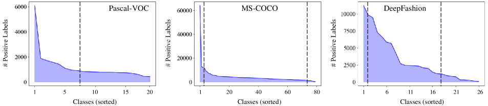
Figure 7: Imbalanced labels of the three benchmark datasets.

$\epsilon$	​​​​​​​​​Mis. $20\%$​​​​​​​​​	​​​​​​​​​Mis. $40\%$​​​​​​​​​	$\epsilon$	​​​​​​Missing Label​​​​​​
​1.000​​	82.5	77.8	​​0.550​​	77.4
​0.975​​	84.3	81.4	​​0.600​​	77.3
​0.950​​	84.0	81.5	​​0.700​​	76.8
​0.900​​	83.7	81.3	​​0.900​​	76.3

Table 7: Parameter search for $\epsilon$ when fixing $\alpha=4.0$.

$\alpha$	All	Many	Medium	Few
​1.0​​	80.3	84.8	81.2	63.2
​2.0​​	81.1	85.6	82.3	60.3
​4.0​​	81.6	85.5	82.6	63.1
​8.0​​	81.3	85.1	82.5	60.1

Table 8: Parameter search for $\alpha$ when fixing $\epsilon=0.975$.

Class Group		MS-COCO					Pascal-VOC
Category	Method	Mis. 20%	Mis. 40%	​​Rand. 20%​​	​​Rand. 40%​​	Single	Mis. 20%	Mis. 40%	​​Rand. 20%​​	​​Rand. 40%​​	Single
Default	BCE Loss	73.1$\pm$0.4	63.8$\pm$0.8	59.8$\pm$0.5	43.5$\pm$0.8	69.7$\pm$1.8	82.9$\pm$0.1	75.4$\pm$0.3	76.3$\pm$0.5	72.0$\pm$5.5	85.7$\pm$0.1
Noisy Labels	Co-teaching	82.5$\pm$0.1	78.6$\pm$0.4	65.5$\pm$0.0	43.6$\pm$0.1	68.1$\pm$1.4	92.5$\pm$0.3	90.9$\pm$0.1	82.6$\pm$0.4	70.0$\pm$0.4	81.9$\pm$1.6
	ASL	82.8$\pm$0.1	80.3$\pm$0.2	75.0$\pm$0.1	66.2$\pm$0.1	73.3$\pm$0.2	91.2$\pm$0.0	86.4$\pm$0.1	90.1$\pm$0.1	74.8$\pm$0.3	86.8$\pm$0.1
Missing Labels	LL-R	80.7$\pm$0.1	75.3$\pm$0.2	74.0$\pm$0.2	69.3$\pm$0.2	74.2$\pm$0.2	87.5$\pm$0.5	83.1$\pm$1.2	85.5$\pm$0.3	78.6$\pm$2.2	89.1$\pm$0.4
	LL-Ct	81.3$\pm$0.0	77.4$\pm$0.1	73.2$\pm$0.3	70.1$\pm$0.1	76.9$\pm$0.1	88.8$\pm$0.5	84.8$\pm$1.4	87.1$\pm$0.2	78.8$\pm$0.3	89.3$\pm$0.1
Proposed	BalanceMix	84.3$\pm$0.1	81.6$\pm$0.3	76.5$\pm$0.1	74.5$\pm$0.1	77.4$\pm$0.1	92.9$\pm$0.1	92.0$\pm$0.0	91.2$\pm$0.1	84.4$\pm$0.1	92.6$\pm$0.1

Table 9: Last mAPs on MS-COCO and Pascal-VOC with standard errors.

Class Group		All			Medium-shot			Few-shot
Category	Method	0%	20%	40%	0%	20%	40%	0%	20%	40%
Default	BCE Loss	87.7	82.9	75.4	94.1	85.3	77.1	84.9	81.8	74.8
Noisy Labels	Co-teaching ​​​​	90.8	92.5	90.9	93.9	94.0	92.8	89.4	91.8	90.0
	ASL	91.4	91.2	86.4	92.9	92.4	80.5	90.8	90.7	88.9
	T-estimator​​​​	91.0	89.5	89.0	92.4	91.9	91.6	90.2	88.5	87.9
Missing Labels	LL-R	81.8	87.5	83.1	92.5	89.6	85.7	77.2	86.6	81.9
	LL-Ct	84.0	88.8	84.8	90.3	90.7	87.9	81.3	87.9	83.5
Proposed	BalanceMix	93.3	92.9	92.0	95.1	94.4	93.6	92.5	92.2	91.3

Table 10: Last mAPs on Pascal-VOC with mislabeling of $0$–$40\%$. The 1st and 2nd best values are in bold and underlined.

Class Group		All			Medium-shot			Few-shot
Category	Method	0%	20%	40%	0%	20%	40%	0%	20%	40%
Default	BCE Loss	87.7	76.3	72.0	94.1	80.0	74.4	84.9	74.8	71.0
Noisy Labels	Co-teaching ​​​​	90.8	82.6	70.3	93.9	87.1	82.8	89.4	80.6	64.9
	ASL	91.4	90.1	74.8	92.9	92.3	87.6	90.8	89.2	69.3
	T-estimator ​​​​	91.0	85.9	70.1	92.4	89.3	80.3	90.2	84.4	65.6
Missing Labels	LL-R	81.8	85.5	78.6	92.5	88.8	83.0	77.2	84.0	76.8
	LL-Ct	84.0	87.1	78.8	90.3	89.3	82.9	81.3	86.1	77.1
Proposed	BalanceMix	93.3	91.2	84.4	95.1	93.8	91.7	92.5	90.0	81.3

Table 11: Last mAPs on Pascal-VOC with random flipping of $0$–$40\%$. The 1st and 2nd best values are in bold and underlined.

D. Detailed Experiment Configuration

All the algorithms are implemented using Pytorch 21.11 and run using two NVIDIA V100 GPUs utilizing distributed data parallelism. We fine-tune ResNet-50 pre-trained on ImageNet-1K for 20, 50, and 40 epochs for Pascal-VOC (a batch size of $32$), MS-COCO (a batch size of $64$), and DeepFashion (a batch size of $64$) using an SGD optimizer with a momentum of 0.9 and a weight decay of $10^{-4}$. All the images are resized with $448\times 448$ resolution. The initial learning rate is set to be $0.01$ and decayed with a cosine annealing without restart. The number of warm-up epochs is set to be 5, 10, and 5 for the three datasets, respectively. We adopt a state-of-the-art Transformer-based decoder (Lanchantin et al. 2021; Liu et al. 2021; Ridnik et al. 2023) for the classification head. These experiment setups are exactly the same for all compared methods.

The hyperparameters for the compared methods are configured favorably, as suggested in the original papers.

• Co-teaching (Han et al. 2018): We extend the vanilla version to support multi-label classification. Two models are maintained for co-training. Instead of using the known noise ratio, we fit a bi-modal univariate GMM to the losses of all instances, i.e., instance-level modeling. Then, the instances whose probability of being clean is greater than $0.5$ are selected as clean instances.

• ASL (Ben-Baruch et al. 2021): Three hyperparameters – $\gamma^{+}$ which is a down-weighting coefficient for positive labels, $\gamma^{-}$ which is a down-weighting coefficient for negative labels, and $m$ which is a probability margin – are set to be $0.0$, $4.0$, and $0.05$, respectively.

• LL-R & LL-Ct (Kim et al. 2022): The only hyperparameter is $\Delta_{rel}$, which determines the speed of increasing the rejection (or correction) rate. The default value used in the original paper was $0.2$ for 10 epochs. Hence, we modify the value according to our training epochs, such that the rejection (or correction) ratios at the final epoch are the same. Specifically, it is set to be $0.1$ for $20$ epochs (Pascal-VOC), $0.04$ for $50$ epochs (MS-COCO), and $0.05$ for $40$ epochs (DeepFashion), respectively.

Regarding the state-of-the-art comparison with ResNet-101 and TResNet-L, we follow exactly the same settings in the backbone, image resolution, and data augmentation (Ridnik et al. 2023). See Table 5 for details.

E. Hyperparameters

BalanceMix introduces two hyperparameters: $\epsilon$, a confidence threshold for re-labeling and $\alpha$, the parameter of the beta distribution for Mixup. We search for a suitable pair of these two hyperparameters based on MS-COCO.

First, we fix $\alpha\!=\!4.0$ and conduct a grid search to find the best $\epsilon$, as summarized in Table 8. Intuitively, a high threshold value achieves high precision in re-labeling, while a low threshold value achieves high recall. For mislabeling, high precision is more beneficial than high recall; thus, the interval of $0.950$–$0.975$ exhibits the best mAP. However, in the missing (single positive) label setup, high recall precedes high precision because increasing the amount of positive labels is more beneficial; thus, the interval of $0.550$–$0.600$ exhibits the best mAP. Overall, we use $\epsilon=0.550$ for the missing label setup, while $\epsilon=0.975$ for other setups.

Second, we fix $\epsilon=0.975$ and repeat a grid search for the best $\alpha$. Table 8 summarizes the mAPs on MS-COCO with a mislabeling ratio of $40\%$. The best mAP for many-shot classes is observed when $\alpha=2.0$. However, the overall mAP of BalanceMix is the best when $\alpha=4.0$ owing to the highest mAP on medium-shot and few-shot classes. Therefore, we use $\alpha=4.0$ in general.

These hyperparameter values found may not be optimal as we validate them only in a few experiment settings, but BalanceMix shows satisfactory performance with them in all the experiments presented in the paper. We believe that the performance of BalanceMix could be further improved via a more sophisticated parameter search.

F. Additional Main Results

Results with Standard Errors

Table 9 summarizes the last mAPs on MS-COCO and Pascal-VOC. We repeat the experiments thrice and report the averaged mAPs as well as their standard errors. These standard errors are, in general, very small.

Mixing coef. $\alpha$	0.0	1.0	2.0	4.0	8.0
Many-shot	85.4	85.6	85.1	85.5	84.8
Few-shot	57.4	60.3	62.4	63.1	63.2

Table 12: Varying $\alpha$ on COCO with mislabeling of $40\%$.

Results on Pascal-VOC

Tables 10 and 11 summarize the mAPs on Pascal-VOC with mislabeing and random flipping. The performance trends are similar to those on MS-COCO except that Co-teaching exhibits higher mAPs than ASL in the mislabeling noise. In Pascal-VOC unlike MS-COCO, the number of positive labels per instance is only two on average. Therefore, the instance-level selection of Co-teaching can perform better than ASL. However, in the random flipping noise where even negative labels are flipped by a given noise ratio, Co-teaching is much worse than ASL. BalanceMix consistently exhibits the best mAPs for all class categories. Regarding T-estimator, it performs much better than BCE Loss and exhibits comparable performance to Co-teaching and ASL, even if 10% of training data is not used for training since it is required for the noisy validation set.

G. Analysis of Label-wise Management

Method	Clean	​​​Mis. 40%​​​	​​​Rand. 40%​​​	Missing ​​
​​​​Co-teaching	82.8	78.6	43.6	68.1
​​​​T-estimator	84.3	80.5	69.9	16.8
​​​​LL-R	82.5	75.3	69.3	74.2
​​​​LL-Ct	79.4	77.4	70.1	76.9
​​​​BalanceMix (wo Min.)​​​​​​​	85.0	80.9	73.0	77.0

Table 13: Analysis of BalanceMix w.o using the minority sampler on MS-COCO.

	Clean Label Selection (C by Eq. (8))				Re-labeling (R by Eq. (9))
Noise Type​​	Mislabel 20%		Mislabel 40%		Mislabel 20%		Mislabel 40%
Training Progress​​​​	Precision	Recall	Precision	Recall	​​Proportion​​	Accuracy	Proportion	Accuracy
25% Epochs	99.2%	85.3%	96.1%	90.5%	10.1%	98.6%	12.0%	98.9%
50% Epochs	99.0%	88.9%	95.5%	92.7%	9.1%	98.6%	11.2%	98.8%
100% Epochs	98.6%	91.5%	94.5%	94.3%	8.3%	98.5%	9.1%	98.5%

Table 14: Clean label selection and re-labeling performance of BalanceMix on MS-COCO: 2nd-5th columns summarize the label precision and label recall of selecting clean labels, and 6th-9th columns summarize the proportion of re-labeled labels and their re-labeling accuracy.

	Clean Label Selection (C by Eq. (8))				Re-labeling (R by Eq. (9))
Noise Type​​	Mislabel 20%		Mislabel 40%		Mislabel 20%		Mislabel 40%
Training Progress​​​​	Precision	Recall	Precision	Recall	​​Proportion​​	Accuracy	Proportion	Accuracy
25% Epochs	99.6%	88.0%	98.2%	91.5%	2.9%	97.4%	2.0%	97.4%
50% Epochs	99.3%	93.6%	97.2%	94.8%	6.9%	98.8%	5.9%	98.8%
75% Epochs	99.2%	94.4%	97.0%	95.5%	8.6%	99.0%	7.0%	99.0%
100% Epochs	99.2%	95.0%	96.7%	95.9%	8.6%	99.1%	6.8%	99.1%

Table 15: Clean label selection and re-labeling performance of BalanceMix on Pascal-VOC: 2nd-5th columns summarize the label precision and label recall of selecting clean labels, and 6th-9th columns summarize the proportion of re-labeled labels and their re-labeling accuracy.

G.1. Mixing with Different Diversity

The diversity is added by mixing the instances from the random sampler with the instances from the minority sampler via Mixup. Thus, when the Mixup coefficient $\alpha$ is $0$, mixing is not performed at all, and the diversity is the lowest. On the other hand, as $\alpha$ becomes larger, minority samples are more strongly mixed with random samples, and the diversity gets higher. As shown in Table 12, increasing the value of $\alpha$ enhances few-shot class performance, but excessive adjustments degrade many-shot class performance; when $\alpha=0$, a low performance of few-shot classes is attributed to the overfitting caused by limited diversity.

G.2. Pure Effect of Label-wise Management

We compare solely the label-wise management with the refinement-based methods (Co-teaching, T-estimator, LL-R, and LL-Ct) by excluding the additional gains from the minority sampler. Thus, we replace the minority sampler of BalanceMix with the random sampler because the refinement-based methods use the random Mixup. Then, the remaining differences of BalanceMix from others are (1) the definition of ambiguous labels and (2) the diminution of their loss based on inferred clean probabilities. Table 13 shows the result of such comparison, clearly showing the pure superiority of our label-wise refinement over other counterparts.

G.3. Label Precision and Label Recall

The label-wise management of BalanceMix involves selecting clean labels and re-labeling incorrect labels. There are four metrics to evaluate clean label selection and re-labeling performance. Regarding label selection, there are two indicators, label precision and recall, of evaluating how accurate and how many clean labels are chosen from noisy labels, respectively (Han et al. 2018; Song et al. 2022). For convenience, let ${\sf C}$ be the set of all selected labels from all noisy labels, and ${\sf L}$ be the set of all clean labels. Then, the label precision and recall are formulated as:

$$\begin{gathered}{\rm Label~{}Precision}={|\{\tilde{y}\in{\sf C}:\tilde{y}=y\}|}~{}/~{}{|{\sf C}|},\\ {\rm Label~{}Recall}={|\{\tilde{y}\in{\sf C}:\tilde{y}=y\}|}~{}/~{}{|{\sf L}|}.\end{gathered}$$ (14)

Regarding re-labeling, we evaluate its performance based on the proportion of re-labeled labels and their re-labeling accuracy. Let ${\sf R}$ be the re-labeled labels among all noisy labels, and ${\sf D}$ be the entire label in data. Then, the proportion and accuracy are formulated as:

$$\begin{gathered}{\rm Relabel~{}Proportion}={|{\sf R}|}~{}/~{}{|{\sf D}|},\\ {\rm Relabel~{}Accuracy}={|\{\tilde{y}\in{\sf R}:\tilde{y}=y\}|}~{}/~{}{|{\sf R}|}.\end{gathered}$$ (15)

Table 14 summarizes their performance on MS-COCO at three different learning progress. For label selection, we evaluate label precision and recall (Han et al. 2018; Song et al. 2022) of the selected clean labels, where they are indicators of how accurate and how many clean labels are chosen, respectively. BalanceMix exhibits very high precision and recall, and the recall increases greatly as training progresses without compromising the precision. For re-labeling, we evaluate the percentage of re-labeled labels and their accuracy. BalanceMix keeps very high re-labeling accuracy in all training phases. Thus, as the model continues to evolve, more clean labels are selected with high precision, and incorrect labels are re-labeled with high accuracy.

Table 15 summarizes their performance on Pascal-VOC at three different learning progress. In Pascal-VOC, BalanceMix exhibits similar trends of label selection, compared when using MS-COCO. However, we observe that the number of re-labeled labels shows a different trend in MS-COCO and Pascal-VOC. The number increases over training epochs in Pascal-VOC, but an opposite trend is observed in MS-COCO. We expect that the re-labeling performance may be associated with the learning difficulty of training data and the number of classes in training data. We will leave further analysis of re-labeling as future work.

Figure 8: Examples of incorrect and missing labels originally contained in MS-COCO. The red labels (incorrect labels) and green labels (missing labels) are detected and corrected by BalanceMix during training.

H. Noisy Labels in MS-COCO

It is of interest to see a significant improvement of BalanceMix on MS-COCO in our state-of-the-art comparison (see Table 5). It turns out that MS-COCO originally has incorrect and missing labels. Fig. 8 shows a few successfully re-labeled examples from MS-COCO by BalanceMix. The first row shows four examples with incorrect labels, and the second row shows four examples with missing labels. As an example with the first image, an oven is mislabeled as a positive label, but it is re-labeled as a negative one by BalanceMix. As an example with the fifth image, a cat is omitted in labeling, but it is re-labeled as a positive one by BalanceMix. Therefore, the state-of-the-art performance of BalanceMix in MS-COCO is attributed to its versatility for real noisy and imbalanced labels.

References

- Arpit et al. (2017) Arpit, D.; Jastrzebski, S.; Ballas, N.; Krueger, D.; Bengio, E.; Kanwal, M. S.; Maharaj, T.; Fischer, A.; Courville, A.; Bengio, Y.; et al. 2017. A closer look at memorization in deep networks. In ICML, 233–242.
- Bai et al. (2021) Bai, Y.; Yang, E.; Han, B.; Yang, Y.; Li, J.; Mao, Y.; Niu, G.; and Liu, T. 2021. Understanding and improving early stopping for learning with noisy labels. In NeurIPS, 24392–24403.
- Bello et al. (2021) Bello, M.; Nápoles, G.; Vanhoof, K.; and Bello, R. 2021. Data quality measures based on granular computing for multi-label classification. Information Sciences, 560: 51–67.
- Ben-Baruch et al. (2021) Ben-Baruch, E.; Ridnik, T.; Zamir, N.; Noy, A.; Friedman, I.; Protter, M.; and Zelnik-Manor, L. 2021. Asymmetric loss for multi-label classification. In ICCV, 82–91.
- Chen et al. (2021) Chen, P.; Ye, J.; Chen, G.; Zhao, J.; and Heng, P.-A. 2021. Beyond class-conditional assumption: A primary attempt to combat instance-dependent label noise. In AAAI, 11442–11450.
- Cole et al. (2021) Cole, E.; Mac Aodha, O.; Lorieul, T.; Perona, P.; Morris, D.; and Jojic, N. 2021. Multi-label learning from single positive labels. In CVPR, 933–942.
- Cubuk et al. (2020) Cubuk, E. D.; Zoph, B.; Shlens, J.; and Le, Q. V. 2020. Randaugment: Practical automated data augmentation with a reduced search space. In CVPRW, 702–703.
- Ding et al. (2022) Ding, Y.; Zhou, T.; Zhang, C.; Luo, Y.; Tang, J.; and Gong, C. 2022. Multi-class Label Noise Learning via Loss Decomposition and Centroid Estimation. In SDM, 253–261.
- Du et al. (2023) Du, Y.; Shen, J.; Zhen, X.; and Snoek, C. G. 2023. SuperDisco: Super-Class Discovery Improves Visual Recognition for the Long-Tail. In CVPR, 19944–19954.
- Durand, Mehrasa, and Mori (2019) Durand, T.; Mehrasa, N.; and Mori, G. 2019. Learning a deep convnet for multi-label classification with partial labels. In CVPR, 647–657.
- Everingham et al. (2010) Everingham, M.; Van Gool, L.; Williams, C. K.; Winn, J.; and Zisserman, A. 2010. The PASCAL visual object classes (VOC) challenge. International Journal of Computer Vision, 88(2): 303–338.
- Ferreira, Costeira, and Gomes (2021) Ferreira, B. Q.; Costeira, J. P.; and Gomes, J. P. 2021. Explainable Noisy Label Flipping for Multi-Label Fashion Image Classification. In CVPRW, 3916–3920.
- Galdran, Carneiro, and González Ballester (2021) Galdran, A.; Carneiro, G.; and González Ballester, M. A. 2021. Balanced-mixup for highly imbalanced medical image classification. In MICCAI, 323–333.
- Guo and Wang (2021) Guo, H.; and Wang, S. 2021. Long-tailed multi-label visual recognition by collaborative training on uniform and re-balanced samplings. In CVPR, 15089–15098.
- Han et al. (2018) Han, B.; Yao, Q.; Yu, X.; Niu, G.; Xu, M.; Hu, W.; Tsang, I.; and Sugiyama, M. 2018. Co-teaching: Robust training of deep neural networks with extremely noisy labels. In NeurIPS, 8536–8546.
- Hu et al. (2018) Hu, M.; Han, H.; Shan, S.; and Chen, X. 2018. Multi-label learning from noisy labels with non-linear feature transformation. In ACCV, 404–419.
- Huang et al. (2019) Huang, J.; Qu, L.; Jia, R.; and Zhao, B. 2019. O2u-net: A simple noisy label detection approach for deep neural networks. In ICCV, 3326–3334.
- Huynh and Elhamifar (2020) Huynh, D.; and Elhamifar, E. 2020. Interactive multi-label cnn learning with partial labels. In CVPR, 9423–9432.
- Kim et al. (2022) Kim, Y.; Kim, J. M.; Akata, Z.; and Lee, J. 2022. Large Loss Matters in Weakly Supervised Multi-Label Classification. In CVPR, 14156–14165.
- Kim et al. (2023) Kim, Y.; Kim, J. M.; Jeong, J.; Schmid, C.; Akata, Z.; and Lee, J. 2023. Bridging the Gap between Model Explanations in Partially Annotated Multi-label Classification. In CVPR, 3408–3417.
- Lanchantin et al. (2021) Lanchantin, J.; Wang, T.; Ordonez, V.; and Qi, Y. 2021. General multi-label image classification with transformers. In CVPR, 16478–16488.
- Li, Socher, and Hoi (2020) Li, J.; Socher, R.; and Hoi, S. C. 2020. DivideMix: Learning with noisy labels as semi-supervised learning. In ICLR.
- Lin et al. (2017) Lin, T.-Y.; Goyal, P.; Girshick, R.; He, K.; and Dollár, P. 2017. Focal loss for dense object detection. In CVPR, 2980–2988.
- Lin et al. (2014) Lin, T.-Y.; Maire, M.; Belongie, S.; Hays, J.; Perona, P.; Ramanan, D.; Dollár, P.; and Zitnick, C. L. 2014. Microsoft COCO: Common objects in context. In ECCV, 740–755.
- Liu et al. (2021) Liu, S.; Zhang, L.; Yang, X.; Su, H.; and Zhu, J. 2021. Query2label: A simple transformer way to multi-label classification. arXiv preprint arXiv:2107.10834.
- Liu et al. (2016) Liu, Z.; Luo, P.; Qiu, S.; Wang, X.; and Tang, X. 2016. DeepFashion: Powering Robust Clothes Recognition and Retrieval with Rich Annotations. In CVPR, 1096–1104.
- Loyola-González et al. (2016) Loyola-González, O.; Martínez-Trinidad, J. F.; Carrasco-Ochoa, J. A.; and García-Borroto, M. 2016. Study of the impact of resampling methods for contrast pattern based classifiers in imbalanced databases. Neurocomputing, 175: 935–947.
- Park et al. (2022) Park, S.; Hong, Y.; Heo, B.; Yun, S.; and Choi, J. Y. 2022. The Majority Can Help The Minority: Context-rich Minority Oversampling for Long-tailed Classification. In CVPR, 6887–6896.
- Ridnik et al. (2023) Ridnik, T.; Sharir, G.; Ben-Cohen, A.; Ben-Baruch, E.; and Noy, A. 2023. ML-Decoder: Scalable and versatile classification head. In WACV, 32–41.
- Shikun et al. (2022) Shikun, L.; Xiaobo, X.; Hansong, Z.; Yibing, Z.; Shiming, G.; and Tongliang, L. 2022. Estimating Noise Transition Matrix with Label Correlations for Noisy Multi-Label Learning. In NeurIPS.
- Song, Kim, and Lee (2019) Song, H.; Kim, M.; and Lee, J.-G. 2019. SELFIE: Refurbishing unclean samples for robust deep learning. In ICML, 5907–5915.
- Song et al. (2022) Song, H.; Kim, M.; Park, D.; Shin, Y.; and Lee, J.-G. 2022. Learning from noisy labels with deep neural networks: A survey. IEEE TNNLS.
- Tarekegn, Giacobini, and Michalak (2021) Tarekegn, A. N.; Giacobini, M.; and Michalak, K. 2021. A review of methods for imbalanced multi-label classification. Pattern Recognition, 118: 107965.
- Trivedi et al. (2017) Trivedi, S. K.; Dey, S.; Kumar, A.; and Panda, T. K. 2017. Handbook of research on advanced data mining techniques and applications for business intelligence. IGI Global.
- Wang et al. (2014) Wang, Q.; Shen, B.; Wang, S.; Li, L.; and Si, L. 2014. Binary codes embedding for fast image tagging with incomplete labels. In ECCV, 425–439.
- Wang, Minku, and Yao (2014) Wang, S.; Minku, L. L.; and Yao, X. 2014. Resampling-based ensemble methods for online class imbalance learning. IEEE Transactions on Knowledge and Data Engineering, 27(5): 1356–1368.
- Wei et al. (2023) Wei, Q.; Feng, L.; Sun, H.; Wang, R.; Guo, C.; and Yin, Y. 2023. Fine-grained classification with noisy labels. In CVPR, 11651–11660.
- Wei et al. (2021) Wei, T.; Shi, J.-X.; Tu, W.-W.; and Li, Y.-F. 2021. Robust long-tailed learning under label noise. arXiv preprint arXiv:2108.11569.
- Whang et al. (2021) Whang, S. E.; Roh, Y.; Song, H.; and Lee, J.-G. 2021. Data Collection and Quality Challenges in Deep Learning: A Data-Centric AI Perspective. arXiv preprint arXiv:2112.06409.
- Wu et al. (2020) Wu, T.; Huang, Q.; Liu, Z.; Wang, Y.; and Lin, D. 2020. Distribution-balanced loss for multi-label classification in long-tailed datasets. In ECCV, 162–178.
- Xia et al. (2022) Xia, X.; Liu, T.; Han, B.; Gong, M.; Yu, J.; Niu, G.; and Sugiyama, M. 2022. Sample selection with uncertainty of losses for learning with noisy labels. In ICLR.
- Yuan et al. (2023) Yuan, J.; Zhang, Y.; Shi, Z.; Geng, X.; Fan, J.; and Rui, Y. 2023. Balanced masking strategy for multi-label image classification. Neurocomputing, 522: 64–72.
- Zhang et al. (2018) Zhang, H.; Cisse, M.; Dauphin, Y. N.; and Lopez-Paz, D. 2018. Mixup: Beyond empirical risk minimization. In ICLR.
- Zhang et al. (2020) Zhang, M.; Hu, L.; Shi, C.; and Wang, X. 2020. Adversarial label-flipping attack and defense for graph neural networks. In ICDM, 791–800.
- Zhang et al. (2021) Zhang, S.; Li, Z.; Yan, S.; He, X.; and Sun, J. 2021. Distribution alignment: A unified framework for long-tail visual recognition. In CVPR, 2361–2370.
- Zhao and Gomes (2021) Zhao, W.; and Gomes, C. 2021. Evaluating multi-label classifiers with noisy labels. arXiv preprint arXiv:2102.08427.